Interference-Based Scheduling in Spatial Reuse TDMA12179/FULLTEXT01.pdf · Interference-Based...
147
Interference-Based Scheduling in Spatial Reuse TDMA JIMMI GRÖNKVIST Doctoral Thesis Stockholm, Sweden 2005
Transcript of Interference-Based Scheduling in Spatial Reuse TDMA12179/FULLTEXT01.pdf · Interference-Based...
Interference-Based Scheduling in Spatial ReuseTDMA
JIMMI GRÖNKVIST
Doctoral ThesisStockholm, Sweden 2005
TRITA-S3-RST-0515ISSN 1400-9137ISRN KTH/RST/R--05/15--SE
KTH Signaler, sensorer och systemSE-100 44 Stockholm
SWEDEN
Akademisk avhandling som med tillstånd av Kungl Tekniska högskolan framläggestill offentlig granskning för avläggande av teknologie doktorsexamen fredagen den14 oktober 2005 klockan 14.00 i sal C1, Electrum, Kungliga Tekniska Högskolan,Isafjordsgatan 22, Kista.
© Jimmi Grönkvist, september 2005
Tryck: Universitetsservice US AB
Abstract
Spatial reuse TDMA has been proposed as an access scheme for multi-hop ra-dio networks where real-time service guarantees are important. The idea is toallow several radio terminals to use the same time slot when possible. A timeslot can be shared when the radio units are geographically separated such thatsmall interference is obtained. The transmission rights of the different users aredescribed with a schedule.
In this thesis we will study various aspects of STDMA scheduling. A com-mon thread in these various aspects is the use of an interference-based net-work model, as opposed to a traditional graph-based network model. While aninterference-based network model is more complex than a graph-based model,it is also much more realistic in describing the wireless medium.
An important contribution of this thesis is a comparison of network modelswhere we show that the limited information of a graph model leads to significantloss of throughput as compared to an interference-based model, when perform-ing STDMA scheduling.
The first part ot this thesis is a study of assignment strategies for centralizedscheduling. Traditionally, transmission rights have been given to nodes or tolinks, i.e., transmitter/receiver pairs. We compare these two approaches andshow that both have undesirable properties in certain cases. Furthermore, wepropose a novel assignment strategy, achieving the advantages of both methods.
Next we investigate the effect of a limited frame length on STDMA sched-ules. We first show that the required frame length is larger for link assignmentthan for node assignment. Further, we propose a novel assignment strategy, thejoint node and link assignment, that has as low frame length requirements asnode assignment but with the capacity of link assignment.
In the last part of this thesis we describe a novel interfence-based distributedSTDMA algorithm and investigate its properties, specifically its overhead re-quirement. In addition we show that this algorithm can generate as good sched-ules as a centralized algorithm can.
iii

iv
Acknowledgment
I am grateful to many people for helping me carry this thesis to completion.First, I wish to thank my advisor Professor Jens Zander. His scientific guidanceand support, especially in structuring my work, has been invaluable.
Many thanks also to Anders Hansson, who has always been there to listento all my odd ideas. Many ideas have matured during our fruitful discussions.
I have appreciated the help of Pelle Zeijlon, both in helping me with theimplementation of the distributed algorithm, but perhaps more the discussionsaround them. It was a great help in making the algorithm more complete.
Thanks also to Ashay Dhamdhere whom I had the pleasure to work withduring a part of this last year. Apart from that working together have been fun,our cooking and eating of Indian cuisine have also been a pleasure.
Furthermore, I would like to thank the present and the former Head of De-partment, Sören Eriksson and Christian Jönsson, as well as my present and for-mer project managers Mattias Sköld and Jan Nilsson, for giving me the oppor-tunity to do this work.
In addition, I am grateful to all my colleagues at the Department of Commu-nication Systems at the Swedish Defence Research Agency (FOI) for providinga pleasant work environment. In particular, I wish to thank the network researchgroup.
Finally, there is Elisabeth, never forgotten.
v

vi
Contents
1 Introduction 11.1 Military communications . . . . . . . . . . . . . . . . . . . . . 11.2 Ad hoc Networks . . . . . . . . . . . . . . . . . . . . . . . . . 31.3 Medium Access Control . . . . . . . . . . . . . . . . . . . . . 41.4 STDMA Scheduling . . . . . . . . . . . . . . . . . . . . . . . 51.5 Research Area and Previous Work . . . . . . . . . . . . . . . . 81.6 Research Strategy and Contributions . . . . . . . . . . . . . . . 12
1.6.1 Delimitations . . . . . . . . . . . . . . . . . . . . . . . 131.7 Related Work . . . . . . . . . . . . . . . . . . . . . . . . . . . 141.8 Outline of the Thesis . . . . . . . . . . . . . . . . . . . . . . . 15
2 Network Model 172.1 The OSI Model . . . . . . . . . . . . . . . . . . . . . . . . . . 172.2 Data Link layer and Physical Layer . . . . . . . . . . . . . . . . 192.3 Interactions with the Link Layer . . . . . . . . . . . . . . . . . 212.4 Transport and Network Layer . . . . . . . . . . . . . . . . . . . 222.5 Routing assumptions for Mobile Networks . . . . . . . . . . . . 252.6 Traffic Estimations . . . . . . . . . . . . . . . . . . . . . . . . 252.7 Performance Measures . . . . . . . . . . . . . . . . . . . . . . 26
3 Node and Link Assignment 293.1 STDMA scheduling . . . . . . . . . . . . . . . . . . . . . . . . 293.2 Link Assignment . . . . . . . . . . . . . . . . . . . . . . . . . 323.3 Node Assignment . . . . . . . . . . . . . . . . . . . . . . . . . 333.4 Analysis . . . . . . . . . . . . . . . . . . . . . . . . . . . . . . 34
3.4.1 Maximum throughput for link assignment . . . . . . . . 353.4.2 Maximum throughput in node assignment . . . . . . . . 36
vii
3.4.3 An approximative formula for the network delay . . . . 373.5 Evaluation and Results . . . . . . . . . . . . . . . . . . . . . . 38
3.5.1 Unicast Traffic . . . . . . . . . . . . . . . . . . . . . . 393.5.2 Broadcast Traffic . . . . . . . . . . . . . . . . . . . . . 43
3.6 Conclusions . . . . . . . . . . . . . . . . . . . . . . . . . . . . 44
4 Extended Transmission Rights 474.1 LET principle . . . . . . . . . . . . . . . . . . . . . . . . . . . 474.2 Basic Properties . . . . . . . . . . . . . . . . . . . . . . . . . . 504.3 Analysis . . . . . . . . . . . . . . . . . . . . . . . . . . . . . . 534.4 Evaluation and Results . . . . . . . . . . . . . . . . . . . . . . 54
4.4.1 Unicast Traffic . . . . . . . . . . . . . . . . . . . . . . 544.4.2 Broadcast Traffic . . . . . . . . . . . . . . . . . . . . . 57
4.5 Concluding remarks . . . . . . . . . . . . . . . . . . . . . . . . 58
5 Model Comparison 615.1 Graph-based Network Model . . . . . . . . . . . . . . . . . . . 61
5.1.1 Two-level-graph-based scheduling . . . . . . . . . . . . 635.2 Results . . . . . . . . . . . . . . . . . . . . . . . . . . . . . . . 645.3 Concluding remarks . . . . . . . . . . . . . . . . . . . . . . . . 67
6 Effect of Frame Length– Joint Node and Link Assignment 696.1 A centralized algorithm . . . . . . . . . . . . . . . . . . . . . 696.2 Results for Node And Link Assignment . . . . . . . . . . . . . 706.3 Joint Node-Link Assignment . . . . . . . . . . . . . . . . . . . 73
6.3.1 Sharing the Capacity of the Node-Assigned Slot . . . . 746.3.2 Handling Links with Equal Priority values . . . . . . . . 75
6.4 Some results on this . . . . . . . . . . . . . . . . . . . . . . . . 766.5 Some conclusions . . . . . . . . . . . . . . . . . . . . . . . . . 78
7 Distributed Information – How to schedule Efficient? 797.1 Wanted Properties . . . . . . . . . . . . . . . . . . . . . . . . . 797.2 An Interference-Based Distributed Algorithm . . . . . . . . . . 83
7.2.1 Link States . . . . . . . . . . . . . . . . . . . . . . . . 847.2.2 Link Priority . . . . . . . . . . . . . . . . . . . . . . . 857.2.3 Theft of Time slots . . . . . . . . . . . . . . . . . . . . 857.2.4 Choice of time slots . . . . . . . . . . . . . . . . . . . 867.2.5 When do we have a re-scheduling? . . . . . . . . . . . . 87
viii
7.3 What information does a node need? . . . . . . . . . . . . . . . 897.3.1 Continues Variables . . . . . . . . . . . . . . . . . . . 927.3.2 Consequences of limited information . . . . . . . . . . 92
7.4 Instantaneous Maximum Throughput . . . . . . . . . . . . . . . 937.5 Conclusions . . . . . . . . . . . . . . . . . . . . . . . . . . . 95
8 Distributed Information–At what cost? 978.1 What Information Must Each Node Send and to Which Receivers? 978.2 Message Size . . . . . . . . . . . . . . . . . . . . . . . . . . . 1038.3 How Often Are These Messages Sent? . . . . . . . . . . . . . . 1048.4 Exactly How Are Each of These Messages Sent? . . . . . . . . 1058.5 What Affects the Overhead? . . . . . . . . . . . . . . . . . . . 1068.6 Feedback and Stability–Discussion . . . . . . . . . . . . . . . 1078.7 Parameter Settings . . . . . . . . . . . . . . . . . . . . . . . . 109
8.7.1 Imax Threshold . . . . . . . . . . . . . . . . . . . . . . 1108.7.2 Theft Threshold . . . . . . . . . . . . . . . . . . . . . . 1118.7.3 State Threshold . . . . . . . . . . . . . . . . . . . . . . 1128.7.4 h Threshold . . . . . . . . . . . . . . . . . . . . . . . 113
8.8 An Alternative Possibility–Removal of States . . . . . . . . . . 1148.9 Frame Length . . . . . . . . . . . . . . . . . . . . . . . . . . . 1158.10 Results for Different γI . . . . . . . . . . . . . . . . . . . . . 1168.11 The Effect of Mobility–Slow Networks . . . . . . . . . . . . . 1178.12 The Effect of Connectivity–Sparse Network . . . . . . . . . . 1178.13 Comparison to Centralized Scheduling . . . . . . . . . . . . . . 1188.14 Future Work and Improvements . . . . . . . . . . . . . . . . . 1208.15 Conclusions . . . . . . . . . . . . . . . . . . . . . . . . . . . . 121
9 Conclusions and Discussion 123
A Simulation Model 125A.1 Generation of networks . . . . . . . . . . . . . . . . . . . . . . 125A.2 Link Gain . . . . . . . . . . . . . . . . . . . . . . . . . . . . . 126A.3 Simulations of Delay and Throughput . . . . . . . . . . . . . . 127
A.3.1 Simulation of network delay . . . . . . . . . . . . . . . 127A.3.2 Simulation of network throughput . . . . . . . . . . . . 129
ix

x
Chapter 1
Introduction
1.1 Military communications
In future military operations, the armed forces must be able to operate against avariety of threats (from heavy armor to irregular forces) and in a variety of en-vironments, including urban, mountainous and forested terrain, under jammingthreats, sometimes while remaining covert. This will require a very flexiblecommand, control and communications system that can be adapted to the pre-vailing situation.
The communication system will be a central part of a future network centricdefence. Fast and reliable exchange of information between different parts ofthe military organization will be essential and international operations will beincreasingly more important as will cooperation with other countries militaryforces.
Communications capability must be maintained over extended ranges andinteroperation with strategic-, operational- and tactical-level information sys-tems must be possible in order to support autonomous operations with highlydispersed organizational elements. The network must be scalable to permit useover small as well as large areas of operation, possibly with large number ofusers.
This will require a dynamic re-configurable network that can exploit all sen-sors and information sources available for maximum efficiency so that informa-tion can be quickly acquired and assimilated at all levels of the command’shierarchy.
Furthermore, much of the information and its requirements must be avail-
1
2 Chapter 1. Introduction
able even at the level of the individual soldiers. The system must be able to pro-vide its users with robust communication, situation awareness, planning, task-ing and coordination, precise geolocation and navigation, and possibly otherservices not yet foreseen [1].
Since different parts of the network experience very different situations,these different parts must be able to autonomously adapt to the prevailing lo-cal situations and exploit these for maximum efficiency. Such situations canvary from a merely portable Headquarter LAN to the rapid changes on the bat-tlefield itself. In all situations there may be hostile jammers present, and the lossof any unit is possible.
Even under the most severe conditions, the network must provide each sol-dier with the ability to transmit and receive command and control data at a min-imal information rate, regardless of combat situation, position or environment.The network must also function if divided into sub-segments.
All these requirements means that robust, secure, and efficient wireless com-munication networks will play a very essential part of the future military com-munication network.
To avoid weak points, we do not want to rely on centralized control. Fur-thermore, if communication links break due to mobility or hostile jamming wewant the network to be able to reconfigure itself and find other routes for thetraffic.
These requirements differ considerably from most civilian networks, whichusually are geared to low cost with pre-installed wireless infrastructures. Civil-ian networks are often hierarchical in the sense that mobile units will communi-cate through a central, static node. The loss of this central node leads to networkfailure of all units in the surrounding area.
All services the military communication network will provide must be si-multaneously handled by the system, each with different service demands. Forexample, voice transmissions put high demands on the delay. The human ear isespecially sensitive to long delays, which can come from large delay variations(buffered in the end), large delay mean values or a combination of both. On theother hand, a rather high bit error rate can probably be accepted. Other informa-tion updates may have high demands on the avoidance of bit errors, while delaymay be of lesser importance.
The upholding of these service requirements is usually denoted as Quality-of-Service (QoS) guarantees. QoS can be seen as a performance contract be-tween the network and the application. In a mobile radio network no absoluteguarantees can be given since there is always the possibility that the network
1.2. Ad hoc Networks 3
separates into more than one network. However, in this case QoS can be seenas best effort in the sense that the network will achieve the performance agreedupon as long as it is at all possible.
Although it is not possible to foresee all services that will be required inthe future, some of the basic requested services today will most likely also berelevant in the future. In [2], three services are described as particularly inter-esting: group calls, situation awareness, and intranet connections. Group callsare generally considered to be the most important of these services. Group callsrequires a guaranteed low delay, i.e. an upper bound on the time it takes to trans-mit a message from the source to destination or an upper bound on the varianceof the delay (jitter).
A specific example of one scenario where all previous mentioned require-ments and services are necessary is a mechanized battalion, consisting of a num-ber of highly mobile tanks. In this case all communication platforms are vehi-cles, which means that power supply and computational capacity may not be themost limiting factors. However, mobility may be rapid even in difficult terrain.
One type of network that have the potential of fulfilling these requirementsis ad hoc-networks.
1.2 Ad hoc Networks
An ad hoc network consists of (mobile) radio units (nodes) that are spread outin some (possibly unknown) terrain without any form of pre-planning or fixedinfra-structure. Every node is both transmitter and receiver and can also functionas a relay node for nodes further away (multi-hop functionality), outside directradio transmission range, i.e. nodes close to each other communicate directlywhile nodes further away use intermediate nodes as relay nodes.
Ad hoc networks can be robust and flexible since the loss of one of therelaying nodes can be handled by finding other intermediate nodes that can berelays, no node are essential for the functionality of the network. Furthermore,by relaying traffic we do not need line-of-sight communications between thecommunicating nodes, thereby decreasing necessary transmission power.
Ad hoc networks have been suggested for use in several situations wherethe wired communication infrastructure is not sufficient. Beside the obvious— military communications, it can also be used in emergency situations, e.g.after a earthquake where parts of the wired infrastructure have been destroyedor is lacking power supply. Another is to complement cellular systems in order
4 Chapter 1. Introduction
to extend the range of base stations. In this case we need fewer base stationsresulting in a cheaper fixed infra-structure.
There has been research on ad hoc networks since the 70’s, then under thename packet radio networks, but in recent years there have been a considerableincrease in interest for ad hoc networks. Despite this, there is still problems thatneed to be solved before they can be efficiently used in our military scenarios.
One problem is caused by the multi-hop functionality itself. The relaying oftraffic can enable communication between units further away than what wouldotherwise be possible, but it also introduces the problem of finding the path fromsource to destination. This problem is generally referred to as routing and it hasgotten a lot of attention from researchers. The problem is that ad hoc networksusually changes much faster than other networks and new paths must constantlybe found without too large overhead. See for example [3] for an overview ofdifferent routing methods in ad hoc networks.
Another important design issue is Medium Access Control (MAC), i.e. howto avoid or resolve conflicts due to simultaneously transmitting radio units. Lessresearch then for routing have been done here and this will be our main area.
Before we discuss MAC in more detail we can also mention some otherissues of importance for the performance of ad hoc networks. One of them isthe previously mentioned QoS. The rapid changes in an ad hoc network makesreliable guarantees, delays or other, difficult. It is probably necessary to solvethis problem on all levels of the communication system. We can for exampledemand that both routing and MAC attempt to give guarantees. For routing thismeans finding appropriate ways (in terms of what should be guaranteed) and forMAC it may for example mean reservations or prioritizing important data.
Another issue that also is important to solve is security. Ad hoc networks aresupposed to function autonomously without any centralized unit, it is thereforedifficult to use methods that exists for fixed networks. However, this is also anissue we will not study further in this work.
1.3 Medium Access Control
Traditionally, MAC protocols for ad hoc networks are based on contention-based access methods, i.e. a user attempts to access the channel only whenit actually has packets to send. The user has no specific reservation of a chan-nel and only tries to contend for or reserve the channel when it has packets totransmit. This has clear advantages when the traffic is unpredictable. More
1.4. STDMA Scheduling 5
specifically, the most frequently used protocols are based on carrier sense mul-tiple access (CSMA) [4], i.e. each user monitors the channel to see if it is used,and only if it is not will the user transmit. However, this is done in the transmit-ter while collisions appear in the receiver. This can lead to the so-called hiddenterminal problem. A way around this is to first transmit a short request-to-send(RTS) and then only send the message if a clear-to-send (CTS) is received. Thisis the general principle of the IEEE 802.11 standard [5], which at present is themost investigated and used MAC protocol. However, several RTS can be lost ina row which makes delay guarantees difficult.
Efforts have been made to guarantee QoS in CSMA-based medium MAC,see e.g. [6], but contention-based medium access methods are inherently inap-propriate for providing QoS guarantees.
One of the most important QoS parameters in many applications that arespecifically sensitive to the MAC is the delay guarantees previously mentioned.
One approach where delay bounds can be guaranteed is time division multi-ple access (TDMA), i.e. the time is divided into time slots and each user receivesits own time slot.
Unfortunately, in sparsely connected networks this is usually inefficient.But, due to the multihop properties, the time slots can often be shared by morethan one user without conflicts. This will automatically be the case with dy-namic MAC protocols like CSMA, since a user’s access to the channel only willaffect a local area.
However, to achieve both high capacity and delay guarantees one can usespatial reuse TDMA (STDMA) [7], which is an extension of TDMA wherethe capacity is increased by spatial reuse of the time slots, i.e., a time slot canbe shared by radio units geographically separated so that small interference isobtained.
1.4 STDMA Scheduling
The problem is to design STDMA schedules that fulfill required properties, e.g.minimizing delay or being able to update the schedules in a distributed fashion.An STDMA schedule describes the transmission rights for each time slot.
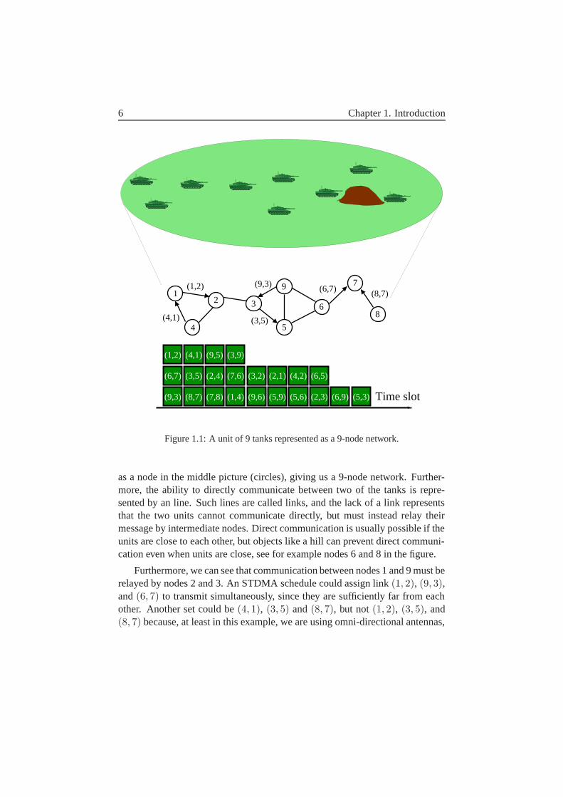
Before we go into more detail we will show a small example of how we cango from a scenario with tanks to an STDMA schedule. In the top part of Figure1.1 we see a group of nine tanks heading to the right.
Now, to represent this as a radio network each of these tanks will be shown
6 Chapter 1. Introduction
(4,1)
(1,2) (9,3)
(3,5)
Time slot(8,7)
(2,1) (6,5)
(1,2)
(6,7)
(9,3)
(4,1)
(3,5)
(9,5)
(2,4)
(7,8)
(3,9)
(7,6)
(1,4)
(3,2)
(9,6) (5,9)
(4,2)
(5,6) (2,3) (6,9) (5,3)
631
4
2
5
9
8
(8,7)(6,7)7
Figure 1.1: A unit of 9 tanks represented as a 9-node network.
as a node in the middle picture (circles), giving us a 9-node network. Further-more, the ability to directly communicate between two of the tanks is repre-sented by an line. Such lines are called links, and the lack of a link representsthat the two units cannot communicate directly, but must instead relay theirmessage by intermediate nodes. Direct communication is usually possible if theunits are close to each other, but objects like a hill can prevent direct communi-cation even when units are close, see for example nodes 6 and 8 in the figure.
Furthermore, we can see that communication between nodes 1 and 9 must berelayed by nodes 2 and 3. An STDMA schedule could assign link (1, 2), (9, 3),and (6, 7) to transmit simultaneously, since they are sufficiently far from eachother. Another set could be (4, 1), (3, 5) and (8, 7), but not (1, 2), (3, 5), and(8, 7) because, at least in this example, we are using omni-directional antennas,
1.4. STDMA Scheduling 7
and the transmission of node 3 would interfere with the reception of node 2.
In the bottom part of the figure we show a possible schedule where each linkreceives one time slot each, as can be seen, at least ten time slots will be neededsince the ten directed links between the four nodes in the center cannot sharetime slots.
Unfortunately, the nodes will be moving, and nodes that can transmit simul-taneously without conflict at one moment will probably not be able to do solater. Returning to the above example we can see that if tank 3 moves slowerthan the three tanks to the left, the transmission of node 1 will eventually createsufficient interference when node 3 receives on link 2 so that links 1,2, and 3cannot share the same time slot anymore.
Therefore, the STDMA schedule must be updated whenever something changesin the network. This can be done in a centralized manner, i.e. all information iscollected into a central node, which calculates a new schedule. This schedule isthen propagated throughout the network. The schedules designed this way canbe very efficient because the central node has all information about the network.
However, for a fast-moving network this is usually not possible. By thetime the new schedule has been propagated it is already obsolete, due to nodemovements. Furthermore, it is not a robust solution, as the loss of the centralnode can be devastating for network communications.
Another way to create STDMA schedules is to do it in a distributed man-ner, i.e. when something changes in the network, only the nodes in the localneighborhood of the change will act on it and update their schedules without theneed to collect information into a central unit. In this thesis we will look at bothmethods.
In the above example, all transmission rights are assigned to the links, i.e.both transmitting and receiving nodes are determined in advance when the sched-ule is created. This is called link assignment or link activation. An alternativewould be to assign transmission rights to the nodes instead. In this case onlythe node is scheduled to transmit in the time slot. Any of its neighbors, or all,can be chosen to be the receiving node. This is called node assignment or nodeactivation.
Generally, node assignment is used for broadcast traffic, and link assignmentis used for unicast traffic. However, in the multipurpose networks of the future,the network must be able to handle both these types of traffic simultaneously,which means that it would be preferable if one assignment strategy can be usedfor all traffic types.
8 Chapter 1. Introduction
1.5 Research Area and Previous Work
In this section we will go further into the problems that have been studied forSTDMA and from this motivate the specific problems we have chosen to inves-tigate in this thesis. In the next section we will describe our research problemsin greater detail.
The problems surrounding the design of STDMA schedules are well ad-dressed in the literature, but areas remain that need more work.
Networks Models
In order to determine which nodes or links that can transmit at the same timewhen we do the scheduling, we need a description of the network. We usuallydenote such a description with a network model. The network models used bySTDMA algorithms have varied in complexity.
Most algorithms assume that transmission ranges are limited (usually circu-lar), and beyond this no interference is caused. This allows the problem to betransformed into a graph-theoretical problem, i.e. the network is represented asa directed graph as we did in the previous section. In this graph, an edge be-tween two nodes indicates that they can communicate with each other directly,and the lack of an edge indicates that they cannot affect each other even as in-terferences. This is commonly referred to as the Protocol Interference Model,see for example [7, 8, 9].
Using this model, scheduling can be transformed into the coloring of thenodes or links in a graph, which can be solved with the help of graph theory.This model thereby makes it simple to create STDMA algorithms. In addition,the maximum distance nodes can effect each other is two hops, which makesit easy to design distributed algorithms. However, a disadvantage is that thismodel does not describe the wireless medium very well as it does not take intoconsideration capture or that the combination of interference from several nodescan cause transmissions to fail.
A more complex network model uses a two-level graph model, see e.g. [10].Here interference edges are added, meaning that there is not sufficient signalpower to receive the packet without error, but it is strong enough to interferewith reception from other users. This model gives a better description of thenetwork and is still useful for a mobile scenario where the schedule must beupdated often.
A more realistic, although even more complex, model is the use of the
1.5. Research Area and Previous Work 9
signal-to-interference ratio, Interference-Based Scheduling. This is also knownas the Physical Interference Model. In this case, a node is assumed to be able toreceive a packet without error if the received signal strength is sufficient com-pared with the noise and all interfering signals (from simultaneously transmit-ting nodes in the network). The first use of this model for STDMA schedulingthat we have found is [11].
The use of the Physical Interference Model is the main focus of this thesis.One reason to this is that it gives a so much better description of the networkthan a graph model. We will generally use interference-based scheduling for allscheduling in this thesis.
The only exception to this is a comparison of network models. Becauseso many algorithms have assumed the use of the Protocol Interference Model,the comparison of the efficiency of these models is one of the research areas inthis thesis. In chapter 5, we will show that graph scheduling can cause severeproblems.
It should be noted, however, that there have also been other approaches tousing graph-based scheduling. In [12] a truncated graph model is used that givesprobabilistic guarantees for the throughput by bounding the maximum numberof simultaneous transmitting units.
Assignment Strategies and Minimizing Frame Length
Since both broadcast traffic and unicast traffic have been considered important inad hoc networks, most work on STDMA has generally assumed the two typesof assignment strategies previously mentioned, i.e. node assignment and linkassignment.
Node assignment have also been called node activation or broadcast schedul-ing. Examples of algorithms that generate node assignment schedules can befound in [8, 13, 14, 15, 16]. Link assignment is often referred to as link activa-tion, and examples of such algorithms can be found in [17, 18, 19, 20].
In practice, both assignment strategies are similar so it is usually simpleto design algorithms for both strategies if an algorithm is designed for one ofthem, which has, for instance, been done in [21, 22]. Another example is [23],in which algorithms for both link and node scheduling are described that focuson generation on short schedules. In [24] a more general description of theassignment problem is presented. The different assignment methods are seen asconstraints in a unified algorithm for the assignment problem given in the paper.
The most common research problem in respect of STDMA has probably
10 Chapter 1. Introduction
been finding algorithms that generate schedules that give each node or link atime slot with as short a schedule as possible. For arbitrary graphs, this hasbeen shown to be an NP-complete problem [25, 26] for both link and nodeassignment. To overcome this the radio networks can instead be modeled asrestricted graphs, for example trees, planar graphs or close to planar graphs forwhich it is easier to find solutions, see [27] for an overview.
However, although node scheduling has generally been assumed to be usedfor multicast traffic and link scheduling has been assumed to be used for unicasttraffic, this does not provide the full picture. Little work exists that studies whichof these assignment strategies is preferable in different scenarios with differenttypes of traffic. In [28], the different properties of node and link assignmenthave been studied in respect of schedules in which nodes or links are assignedone slot each. In this they find that node assignment is preferable for all trafficloads.
Traffic Sensitivity
However, giving each node or link a single time slot is not necessarily good.There is considerable variation of traffic over the different links of the networkdue to the relaying of traffic in multi-hop networks. An STDMA algorithmmust adapt to this and give some nodes more capacity (time slots) in order tobe efficient. Algorithms that do this are usually denoted as traffic sensitive ortraffic controlled. The ability to give some nodes or links extra time slots relatedto the traffic loads on the links has been considered in several papers, see e.g.[17, 29].
Furthermore, studies on traffic sensitivity have also shown that it improvescapacity considerably compared with giving each node or link a single time slot[11, 30].
The results in [28] are therefore somewhat limited because traffic sensitiv-ity is less of a problem for node assignment as there is less variation of thetraffic over the nodes than the links. A comparison under the assumption oftraffic sensitivity will be studied in this thesis. We will show that this gives adifferent result, namely that link assignment can achieve higher throughput thannode assignment. Furthermore, we have chosen to use traffic sensitivity for allscheduling in the thesis.
As we will see, neither node assignment or link assignment will be sufficientin all situations so an important part of the thesis will focus on the suggestion ofnew assignment strategies with better performance.
1.5. Research Area and Previous Work 11
Centralized and Distributed Algorithms
We have left one of the most important problem areas regarding STDMA untilnow. The issues concerns how to design algorithms that can generate schedulesin a distributed manner. There are still many reasons why centralized schedul-ing can be useful. For example, for static networks, a schedule can be generatedcentrally and be distributed to the nodes in the network. However, the main rea-son we study centralized algorithms in this thesis is that it gives us an upper limiton performance and provides some ideas about which properties are importantwhen we do the distributed scheduling. Many such centralized algorithms havebeen suggested, see for example [14, 19, 31].
However, in most scenarios where STDMA is envisioned, for example inthis thesis, mobility is assumed. Being able to update the schedule in a dis-tributed manner is often considered vital. Many such algorithms have been sug-gested, see for example [17, 32, 18, 15, 21, 33, 34], but they all assume a graphmodel to describe the network. As previously mentioned, according to sucha model, nodes will only affect each other at a maximum of two hops, whichmakes the distribution of information much simpler than for an interference-based model that may let nodes at much further distance affect each other, de-pending on the terrain . Few distributed algorithms have been implemented intofunctional systems, but one, USAP [21], is used for to generate multi-channelSTDMA schedules in the soldier phone radio [35] that is designed as an ad hocradio for military use in mobile environments.
No fully distributed STDMA algorithm that can generate schedules basedon the physical Interference Model exists, and the first step towards such a al-gorithms will be an important part of this thesis.
In addition we can return to the previous problem regarding traffic sensitiv-ity, but now specifically for distributed algorithms.
For distributed scheduling, traffic control is only rarely included. Althoughmany algorithms include the ability to assign more than one time slot to a linkor node, cf. [36, 37], a more specific description of how and when some of thelinks receive extra time slots is usually omitted.
One exception is [38] which attempts to generate fair time slot allocationsfor link assignment given traffic demands on each link. Another is [39], whereeach link can request a bandwidth, although the actual bandwidth it receives isproportional to its request compared with the other links’ requests.
Another solution is described in [18], where virtual circuits are assignedtime slots (or rather each link along the virtual circuit). This gives traffic sensi-
12 Chapter 1. Introduction
tivity because a link can carry more than one virtual circuit.
1.6 Research Strategy and Contributions
We will study the behavior of STDMA in two different types of mobility sce-narios. First, centralized algorithms in static networks (in terms of both nodemobility and traffic). We use centralized scheduling to give us an upper limit onperformance, and to provide some ideas about which properties that are impor-tant when we do the scheduling.
Second, we will study interference-based distributed scheduling in mobilescenarios. We will also describe which properties a distributed STDMA algo-rithm should have in order to be efficient. No existing STDMA algorithm canfulfill all these properties, although USAP [36] fulfills several of them. Investi-gations of distributed STDMA will give us a better picture of how well STDMAperforms.
The present thesis consists of the following studies:
1. We compare the two most common assignment methods used today, i.e.node and link assignment. This comparison is performed both in an an-alytical manner and via simulations, in order to determine when nodeor link assignment should be used. We will show that link assignmentbehaves better for high traffic loads, achieving a higher throughput forunicast traffic. However, this comes at a cost of higher delay than nodeassignment for low traffic loads. Our results also indicate that only thesize and the connectivity of the network are necessary to determine wheneach of these methods should be used.
This has been published in [40, 41].
2. We suggest a novel assignment strategy that achieves the advantages ofboth link assignment and node assignment. Our proposed strategy isbased on a link schedule, but in which transmission rights are extended.This strategy is evaluated in comparison with the other two methods byusing approximations and simulations.
This has been published in [42, 43, 41].
3. We investigate the loss of efficiency (in terms of throughput) when theSTDMA algorithm only has knowledge about the two-level graph modelof the network compared with having full knowledge of the attenuation
1.6. Research Strategy and Contributions 13
between all pairs of nodes. We show that the traditional graph-basedscheduling can lead to significant loss of throughput.
A somewhat different approach to this has been published in [44].
4. We investigate the effect of a limited frame length. We will show that therequired frame length is larger for link assignment than for node assign-ment, but we also suggest a novel assignment strategy–joint node and linkassignment–that has as low frame length requirements as node assignmentbut with the capacity of link assignment.
This is a joint study in collaboration with Ashay Dhamdhere.
A version of this is submitted to [45].
5. We describe a novel interference-based distributed STDMA algorithmthat can give results as high as what a centralized algorithm can. Thisis done for an investigation on how to efficiently handle (use) distributedinformation. This is mainly published in [46] and [47].
6. We show how to reduce the overhead requirement of the above describedalgorithm by choosing good parameter settings. With overhead require-ment we mean how much control information is required to convey thedesired network information. This can be done to indicate how muchnetwork information should be transferred for different networks.
This is not yet published.
1.6.1 Delimitations
We will not study all extra features that can be added in order to further improveSTDMA. Examples of such features are power control, rate control, adaptiveantennas, and similar methods. We have enough parameters to handle withoutthese, but they can further improve STDMA. One goal of this work is to simplifytheir inclusion later.
However, rate control will partly be included for distributed scheduling sincebecause some form of rate control is probably necessary for interference-basedscheduling in mobile networks.
Other practical issues concerning how to make an STDMA scheme workwill not be studied. These include slot synchronization, exact functionality ofdata link layer, effects of Tx/Rx turnaround time, hostile jammers, and similareffects which do affect the performance of the network.
14 Chapter 1. Introduction
1.7 Related Work
There are also other areas of research for STDMA that are of interest. Thesewill be out of scope for this thesis, but much of the research on STDMA that isbeing performed today is done in the following areas.
Optimal Scheduling
So far most STDMA algorithms (specifically if they are distributed) have beendesigned to give an acceptable solution, rather than a solution that handles thechannel as efficiently as possible under different situations. However, in [19, 48]the optimal scheduling problem was formulated using graph-based scheduling.However, both of these assumed spread-spectrum signal modulation so onlyavoidance of nodes or links transmitting and receiving at the same time wasnecessary.
Only much more recently has more work been done on this, with most ofthe studies using interference-based scheduling. In [49, 50] capacity regionsfor ad hoc networks are studied. One method examined is a time slotted MACsystem, i.e. what we call STDMA. In addition to this, several papers on optimalscheduling, with different assumptions have been published [51, 52, 53, 54, 55,56].
Cross-Layer Issues
Several of the optimization papers also consider cross-layer issues as well, inrespect of both higher and lower layers. Joint scheduling with power controland/or routing are some examples. As these issues are not the main focus of thepresent thesis we will not provide more details about how these papers differ.
Cross-layer issues have not only been studied for optimal scheduling. Powercontrol have been studied in several cases. See [57] as one example. In [58]variable-rate is also added. Distributed power control is used in [59, 60] (thefirst one without scheduling-however)– and with routing in [61].
Adaptive and directional antennas have been studied for centralized schedul-ing in some cases and have been shown to give considerable improvements[62, 63]. Some results for distributed scheduling also exist [64].
So far optimization methods are mainly useful as reference methods, be-cause they require all information about the network and it takes a long timeto calculate the schedules, especially for large networks. In addition, the best
1.8. Outline of the Thesis 15
possible schedule in terms of throughput can be very long in order to handletraffic sensitivity. Finding the best schedule with a given frame length is still avery difficult.
1.8 Outline of the Thesis
In Chapter 2 we describe the network model we have used. We also describe thelayers, according to the OSI model, that are of interest to us, i.e. data link layer,network layer and transport layer. The data link layer describes the functionalityof the links and when a link can be used without conflicts.
The transport layer basically gives us a model of the external traffic of thenetwork, whereas the network layer includes the routing of this traffic. Themain purpose of this is to calculate the traffic on the links and nodes in thenetwork. We also define the evaluation parameters, which are the average end-to-end packet delay and the maximum throughput.
The rest of the thesis can be divided into two parts: centralized schedulingand distributed scheduling. In Chapters 3 to 6 we will deal with centralizedscheduling for static networks. In Chapters 7 and 8 we will study distributedscheduling for mobile networks.
In Chapter 3 we define and exemplify node assignment and link assignment.We also provide approximations for the maximum throughput and the averagepacket delay for these assignment methods. These are then used to compare theefficiency of the algorithms. We conclude the chapter with simulations of delayand throughput to determine how well the approximations work.
In Chapter 4 we describe a novel assignment method LET. Here, too, wegive an approximate formula for the delay and use this in comparison with sim-ulations. These results are then compared to node and link assignment, showingthe advantages of LET.
In Chapter 5, we make a comparison between using the traditional graphmodel when designing an STDMA schedule and using an interference-basedmodel.
In Chapter 6 we study the effect of different frame lengths and introducea new scheduling strategy, joint node and link assignment, that performs wellunder all frame lengths.
Chapter 7 starts the study on distributed scheduling by giving a list of prop-erties. Furthermore, we describe the distributed algorithm that we use. In chap-ter 8 we continue this by studying the overhead traffic required when using this
16 Chapter 1. Introduction
algorithm for a mobile network.Finally, in Chapter 9 we conclude the thesis.In appendix A we present more information about how simulations are per-
formed.

Chapter 2
Network Model
This chapter introduces the network model we use and the assumptions required.These can be divided into two parts: first, the assumptions on the data link layerand then the assumptions from the network and transport layers. The data linklayer is described in the first section. The assumptions on the higher layersdescribe how the traffic is generated and routed.
Furthermore, we also describe how the performance will be evaluated.
2.1 The OSI Model
To reduce design complexity, most networks are organized as stacks of layers,each one on top of the one below it. Each layer offers a set of services to thelayer on top of it, shielding the above layers from details of the implementationof the layer below. The number of layers and content may vary from network tonetwork, but layer l on a node can be seen as it carries out a conversation withlayer l on another node. The rules of this conversation are called the protocol oflayer l. A collection of layers and protocols is called a network architecture.
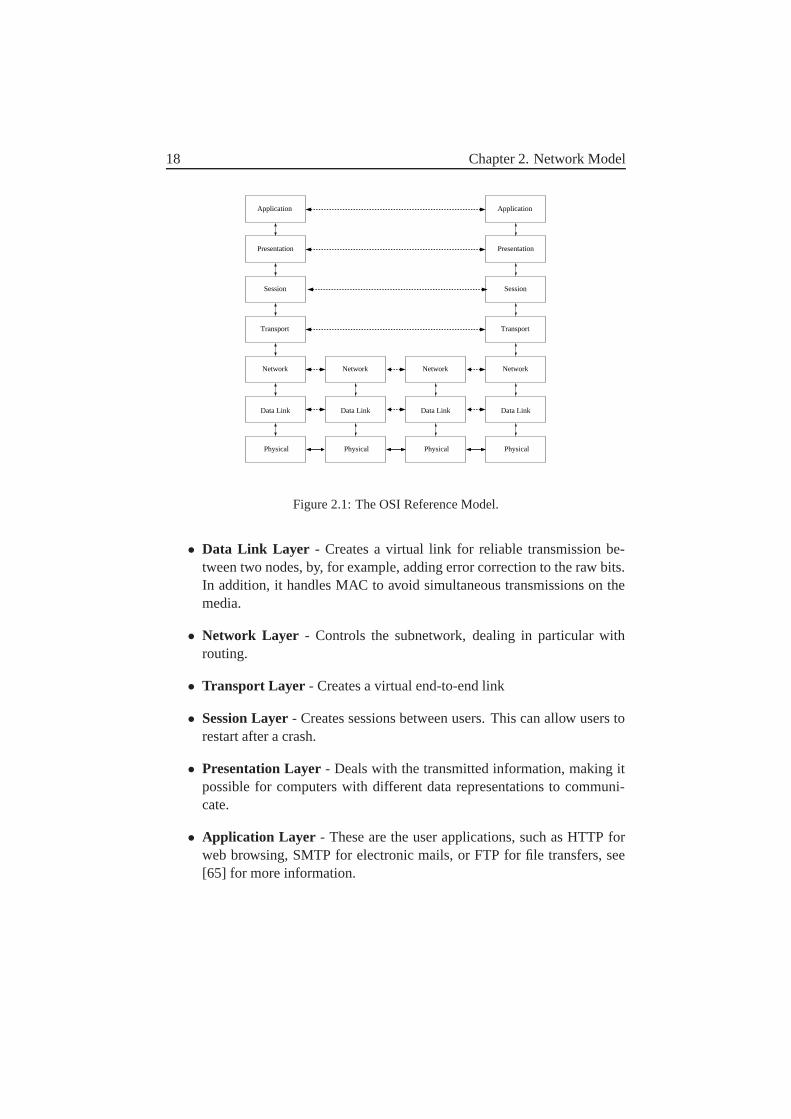
In this thesis we will use the Open System Interconnection (OSI) referencemodel as a basic description of the network architecture, it is not a completearchitecture, however, because the protocols of each layer are not specified.More about network layering and the OSI reference model can be found in [65].The OSI model has seven layers dealing with different issues, see Figure 2.1.The different layers in ascending order are,
• Physical layer - Deals with transmission of raw bits over the channel.
17
18 Chapter 2. Network Model
Application
Presentation
Session
Transport
Data Link
Network
Physical
Application
Presentation
Session
Transport
Data Link
Network
Physical
Data Link
Network
Physical
Data Link
Network
Physical
Figure 2.1: The OSI Reference Model.
• Data Link Layer - Creates a virtual link for reliable transmission be-tween two nodes, by, for example, adding error correction to the raw bits.In addition, it handles MAC to avoid simultaneous transmissions on themedia.
• Network Layer - Controls the subnetwork, dealing in particular withrouting.
• Transport Layer - Creates a virtual end-to-end link
• Session Layer - Creates sessions between users. This can allow users torestart after a crash.
• Presentation Layer - Deals with the transmitted information, making itpossible for computers with different data representations to communi-cate.
• Application Layer - These are the user applications, such as HTTP forweb browsing, SMTP for electronic mails, or FTP for file transfers, see[65] for more information.
2.2. Data Link layer and Physical Layer 19
As can be seen, the four highest layers deals with end-to-end communicationthat is only be needed in the end nodes, whereas the three lowest layers areneeded in all intermediate nodes. In an ad hoc node all layers are necessary..
Since an STDMA schedule controls when a link should be used, it therebyhas protocols in the network layer as routing on top of it and the specific linkissues in the Data Link Layer and Physical Layer below it.
2.2 Data Link layer and Physical Layer
The radio network considered, consists of a number of radio units spread outin some terrain. If the received signal power from one radio unit is sufficientcompared in relation to noise and interfering signal power, it is assumed thatany two radio units can communicate, i.e., establish a link.
In this section we describe our model for the data link layer and physicallayer. In essence, it is an interference-based model of the radio network, whichis represented by a set of nodes V and the link gain G(i, j) between any twodistinct nodes vi and vj , i = j.
For the link level we will make the following assumptions:
• All antennas are isotropic.
• All nodes use equal transmission power.
• There is only one fixed required BER on the links.
• Slot synchronization is perfect.
• All packets are of equal length.
• A node cannot transmit more than one packet in a time slot and a nodecannot receive and transmit simultaneously in a time slot.
The assumption on isotropic antennas and equal transmission power is mainlyfor simplicity, but in section 4.2 we will present a brief discussion of the con-sequences of directional antennas and varying transmission power specified onLET, since this assignment strategy will be affected most by these assumptions.
For any two nodes, vi and vj where vi is the transmitting node and vj = vi,we define the signal-to-noise ratio (SNR), Γij , as
Γij =PiG(i, j)
Nr, (2.1)

20 Chapter 2. Network Model
(i,j)v vi j
Figure 2.2: Example of a link.
where Pi denotes the power of the transmitting node vi, G(i, j) is the link gainbetween nodes vi and vj , and Nr is the noise power in the receiver. For conve-nience, we define Γii = 0 corresponding to the physical situations of a node notbeing able to transmit to itself.
We say that a pair of nodes vi and vj form a link (i, j), if the signal-to-noiseratio (SNR) is not less than a communication threshold, γC. That is, the set oflinks in the network, L, is defined:
L = (i, j) : Γij ≥ γC . (2.2)
Links are graphically depicted as in Figure 2.2.For a set of links, L ⊆ L, we define the transmitting nodes:
VT(L) = vi : (i, j) ∈ L .
For any link, (i, j) ∈ L, we define the interference as follows
IL(i, j) =∑
vk∈VT(L)\vi
PkG(k, j). (2.3)
Furthermore, we define the signal-to-interference ratio (SIR):
ΠL(i, j) =PiG(i, j)
(Nr + IL(i, j)). (2.4)
We assume that any two radio units can communicate a packet without errorif the SIR is not less than a reliable communication threshold, γR. A scheduleS is defined as the sets Yt, for t = 1, 2, . . . , T , where T is the period of theschedule. The sets Yt contain the nodes or links assigned time slot t. A scheduleis called conflict free if the SIR is not less than the threshold γR for all receivingnodes in all sets Yt.
However, due to mobility and limited information conflict-free schedules arevery difficult to create and uphold. In order to make comparisons for distributed
2.3. Interactions with the Link Layer 21
scheduling we assume that links that have a lower SIR than γR in a time slot candecrease its data rate as compared to the nominal data rate RN used by linkswith SIR above γR, i.e.
SIR
γR=
Used RateRN
, (2.5)
The choice of these thresholds is of course dependent on several factors,such as the actual modulation method of the signal, properties of the receivernoise, data rate and required BER.
The threshold γR will be determined by the factors described above. How-ever, these factors only decide the lowest possible γC. That is, we can choosea higher γC, thereby excluding some node pairs from communicating with eachother. By doing this we can create an interference margin so that all links canhandle some interferences. However, this comes at the price of longer routesand the risk that the network will divide into sub-segments. For simplicity wewill assume that γR=γC for centralized scheduling. For distributed schedulingwe may need the margin due to limited information and in these cases we willuse γC=1.5γR.
We have also chosen γR equal to 10 in all simulations.
2.3 Interactions with the Link Layer
The network model we have described in this chapter is somewhat simplistic(although more complex than a graph model). In reality, all packets will not beperfectly received if the SIR is above γC , and all packets will not be lost justbecause SIR is below the threshold. If the sent packets had infinite size, suchassumptions would be more accurate.
In addition, exact path gains will not be available and fast and slow fadingwill complicate the situation even further. An exact representation on the de-tails of the link is difficult to obtain and even if we could get such informationfrom the links in the network, an STDMA algorithm could not handle such fastchanges anyway.
Instead, we have to hide the volatility of the link from the MAC protocol.The link gain given from lower layer will be an expected average. Variable datarates for the link (as seen from STDMA point of view) must be average datarates, not what actually is transmitted on the link. An adaptive radio node mayactually change data rate on the link from one time slot to the next (in extremecases we could even change it within the time slot).
22 Chapter 2. Network Model
The purpose of the STDMA algorithm is to create sets of simultaneouslytransmitting links that can be efficiently handled locally by the links (withoutany further interaction between them in terms of transmitted information).
Nevertheless, the actual functionality of the link will be ignored in this re-port and we will concentrate on the functionality of STDMA when the detailsof the link layer already have been hidden. This will also be the case for evalu-ations.
2.4 Transport and Network Layer
The traffic arriving at the network can be separated into two types. The first isunicast traffic, with a single source and destination. This type of traffic can bethe carrier of many types of information, e.g. file transfer or telephone conver-sations. The second type of traffic is multicast or broadcast, i.e. a packet hasone source but many destinations. With broadcast we mean the entire network.Broadcast traffic is very usual in military networks, e.g. group calls or situationawareness data.
Since all nodes cannot directly communicate with all other nodes in thenetwork, due to limited transmission power, obstacles and large distances, allnodes in the network are assumed to be able to relay packets. In order to do this,each node is assumed to have a routing table with entry’s for all other nodesin the network. We will not elaborate on how this information is obtained butmerely note that the routing will have an effect on the traffic in the network.Unless otherwise stated, we assume that all networks are connected, i.e. there isalways a path between any pair of nodes.
In the following we first discuss the effects of this for unicast traffic and thenthe effects for broadcast traffic.
Unicast traffic assumes that a packet entering the network has only one des-tination. Packets enter the network at entry nodes according to a probabilityfunction, p(v), v ∈ V , and packets exit the network at exit nodes. When apacket enters the network, it has a destination, i.e. an exit node from the net-work. The destination of a packet is modeled as a conditional probability func-tion, q(w|v), (w, v) ∈ V × V , i.e. given that a packet has entry node v, theprobability that the packet’s destination is w is q(w|v). For simplicity we willassume a uniform traffic model, i.e. p(v) = 1/N , and q(w|v) = 1/(N − 1),where N is the number of nodes, N = |V |. This assumption will not affectour results since we use traffic controlled schedules, thereby compensating for
2.4. Transport and Network Layer 23
variations caused by the input traffic model.Let λ be the total traffic load of the network, i.e. the average number of
packets per time slot arriving at the network as a whole. Then, λ/N(N − 1) isthe total average of traffic load entering the network in node vi with destinationnode vj . As the network is not necessarily fully connected, some packets mustbe relayed by other nodes. In such a case, the traffic load on each link can becalculated only when the traffic has been routed.
For unicast traffic we use the shortest route counted in the number of hops,i.e. packets sent between two nodes will always use the path which requiresthe least number of transmissions. If several routes of the same length exist, allpackets between two specific nodes will always use the same route.
The reason why this routing strategy is used, except for its simplicity, is thatthis minimizes the number of retransmissions needed before a packet reachesthe destination. Since we for routing (scheduling is not yet done) are assuminga fixed data rate on the links, it would be difficult to take advantage of a strategywhich uses a longer route, since we would have to generate schedules with amuch better spatial reuse to compensate for this.
Now, let Ru denote the routing table for unicast traffic, where the list entryRu(v, w) at v, w is a path pvw from entry node v to exit node w, where pvw isgiven by the routing algorithm described above. Let the number of paths in Ru
containing the directed link (i, j) be equal to Λij . From now on, we will callthis parameter the relative traffic on link (i, j).
Comment: For non-uniform traffic the relative traffic should be weightedwith the traffic load on each path rather than just using the number of paths.
Further, let λij be the average traffic load on link (i, j). Then λij is givenby
λij =λ
N(N − 1)Λij .
Moreover, we have, λi as the average traffic load on node vi. Here λi isgiven by:
λi =λ
N(N − 1)
∑
j:(i,j)∈L
Λij =λ
N(N − 1)Λi,
where Λi is denoted as the relative traffic of node vi.This can be described in a similar way for broadcast traffic, which assumes
that a packet entering the network has all other nodes as destination. Packetsenter the network at entry nodes according to a probability function, p(v). Wewill also assume a uniform traffic model, i.e. p(v) = 1/N .
24 Chapter 2. Network Model
Again, let λ be the total traffic load of the network, i.e. the average numberof packets per time slot arriving at the network as a whole. Then λ/N is thetotal average of traffic load entering the network in node vi destined to all othernodes.
Radio is an inherent broadcast medium, especially when we are using om-nidirectional antennas. This means that if we are sending a packet, all nodeswithin range can receive the packet if nothing else interferes with them. Sincethe interference allowed in the nodes is determined by the assignment strategy,this means that depending on what assignment strategy that is used this deter-mines the actual traffic that must be transmitted by the nodes. For example,node assignment guarantees that all neighbors are collision-free, meaning thatall neighboring nodes that should receive the packet will do so by a single trans-mission. Link assignment, on the other hand, is a single transmission over alink. If several neighbors should receive the packet, they have to receive a trans-mission each.
We will therefore define the average traffic of a node as the average numberof different packets that are to be transmitted, regardless of whether they haveone or several destinations. This means that the actual number of transmissionsof the node will be at least this high, which is the case if node assignment is usedsince all packets will reach all their destinations with a single transmission each.Other transmission strategies may require a larger number of transmissions ifmore than one is required for a transmission, e.g. link assignment.
For broadcast traffic, a more advanced routing method must be used than forunicast traffic. As mentioned, radio is an inherent broadcast medium. Depen-dent on which assignment strategy that is used, we can use this to our advantagein a more or less efficient manner. One way of doing this is to minimize thenumber of retransmissions needed for a packet to reach all destinations, i.e. wewant as many neighboring nodes as possible to be reached by each transmission.This can also be described as maximizing the number of leafs in the routing tree.
However, this is a very complex problem, so for simplicity we will use aheuristic algorithm in an attempts to achieve this.
The following creates a routing tree for each node.Initiate by choosing the node as root. Find the node vi with the highest
number of neighboring nodes that is not included in the tree. Include all theseneighboring nodes and the edges from vi to these nodes. This is repeated untilall nodes are included in the tree.
Now, let Rb denote the routing table for broadcast traffic, where the listentry Rb(v) at v is a tree with entry node v as root. Let the number of trees in
2.5. Routing assumptions for Mobile Networks 25
Rb containing the directed link (i, j) be equal to Λij and let the number of treescontaining vertex vi as a non-leaf in the tree be equal to Λi.
Further, let λij be the average traffic load on link (i, j) and λi be the averagetraffic load on node vi . Then λij is given by
λij =λ
NΛij ,
and λi is given by
λi =λ
NΛi.
2.5 Routing assumptions for Mobile Networks
We assume that the routing is perfect and we ignore any necessary overheadcaused by routing traffic. This also means that the routing protocol is assumedto be useful for the multicast transmissions that the STDMA algorithm needs.However, we also assume that the routing protocol reacts to link changes slowerthan the MAC layer is capable of handling, which means that new multicastroutes is available only when the MAC protocol has figured out its new localneighborhood after a change.
This means that between link changes the STDMA algorithm may use therouting protocol for its updates regarding assignment of slots. But when achange takes place, the STDMA algorithm must first work out its new localneighborhood with the old routing information before the routing protocol adaptsto the change.
The routing protocol in each node will have a better picture of how the wholenetwork looks than the local picture from the STDMA algorithm in the node,but the routing protocol will be locally updated through the MAC layer.
2.6 Traffic Estimations
A similar issue is traffic from upper layers. For STDMA to work well, we willneed to have accurate information on traffic loads in order to compensate forthese different traffic loads. However, such information is not always available.Sometimes the applications may give some information, and sometimes we haveto make estimations from the arriving traffic and existing queue lengths.
Such estimations may vary considerably over time, and this informationmay have to be hidden from the STDMA algorithm. How to estimate traffic
26 Chapter 2. Network Model
loads efficiently is a research area in itself and not much has been done forad hoc networks. But because this is outside the scope of this report, we willassume that the actual expected traffic loads are known, as was calculated insection 2.4.
2.7 Performance Measures
One important parameter which will affect the usefulness of a radio network isthe delay of information from source to destination. We will start by discussingdelay for unicast traffic and then discuss how this differs from broadcast traffic.
As seen from a network level, this can be translated to the network delay.Network delay is the expected time, in time slots, from the arrival of a packet atthe buffer of the entry node to the arrival of the packet at the exit node, averagedover all origin-destination pairs. This is the first parameter we will investigate.
To determine the network delay we need the following definitions and nota-tions.
The stochastic variable path delay Dpkl for a path pkl is the time, in time
slots, from the arrival of a packet at the buffer of the arrival node vk to thearrival of the packet at the destination node vl. The stochastic variable edgedelay De
kl(i, j) is the time, in time slots, from the packet arrives at the buffer ofnode vi until it is received by node vj , given that the packet is relayed on pathpkl. This path is deterministically given by the routing algorithm as describedin the previous section.
The path delay is thus the sum of the edge delays of that path,
Dpkl =
∑
(i,j)∈pkl
Dekl(i, j) . (2.6)
The average path delay is a stochastic variable defined as an average overall origin-destination pairs:
1N(N − 1)
∑
(k,l)∈N 2
Dpkl . (2.7)
The network delay D is the expected value of the average path delay, i.e.
D = E[1
N(N − 1)
∑
(k,l)∈N 2
Dpkl] . (2.8)
2.7. Performance Measures 27
Due to the relaying of packets the statistical properties of this variable are com-plicated, and an exact analytical analysis of the network delay is difficult [7].Instead we will use computer simulations to determine this parameter, see ap-pendix A.
We will now compare the above-described with broadcast traffic. When wehave broadcast traffic, each arriving packet has all other nodes as destination.We can now use several different definitions of the packet delay since a packetwill arrive at its destinations at different times. One example would be themaximum delay, i.e. the delay of a packet would be the delay until the arrivalat the last node. However, most nodes will experience a much lower delay. Soinstead we will use the average delay of a packet. The total delay of a packetthat originated at node vi can be written as
Di =1
N − 1
∑
j:(i,j)∈N 2
Dij
where Dij can be described as the path delay between node vi and node vj . Thisis the path in the tree with root vi given by the routing algorithm for broadcastrouting described in the previous section.
The network delay, D, can thus be described with the following expression
D = E[1N
∑
i∈NDi =
1N(N − 1)
∑
(i,j)∈N 2
Dij ],
which is similar to the expression for unicast traffic. However, the actual trafficon the nodes and links will differ, which will result in different delays for thedifferent traffic types.
The demand for higher data rates can often lead to highly loaded networks.One of the advantages of STDMA is that it can function well even under hightraffic loads.
In particular, the largest admissible traffic load yielding a finite networkdelay is highly interesting. This maximum traffic load is commonly referred toas the maximum throughput of the network. We define the maximum throughputas the number λ∗ for which the following expressions hold for all traffic loadsλ,
λ < λ∗ yields bounded Dλ > λ∗ yields unbounded D
Notice, here maximum throughput is the same as uniform capacity, i.e. theminimum bit rate at which any node can communicate with any other node inthe network, because our choice of traffic model.
28 Chapter 2. Network Model
Maximum throughput is the second parameter we study. In mobile scenar-ios this parameter will be a little more complex, a problem is that the capacityof the network will vary over time and even if the expected end-to-end delay fora node pair may be infinite at some moment, due to the fact that capacity is lowat that moment may not result in infinite delay since the network can changeinto a more beneficial situation, allowing all queued packets to reach their des-tination. Still, the expected maximum throughput as a function of time is a veryinteresting parameter to study since it gives us a good indication on whether aspecific STDMA schedule is good or not. Besides, unless we can give any pre-diction about how units move, a good estimator will be that the network doesnot change.
As mentioned, a problem is that the network sometimes is not connected,node pairs in different parts of the network can then not communicate, resultingin infinite expected delay on these paths and no maximum throughput. Thisdoes neither represent the situation very well, nor can any MAC algorithm cando anything about it. In such cases we instead assume that only connected pathsattempts to transmit packets when estimating throughput.
The centralized evaluation will study both network delay and maximumthroughput for different assignment methods in static scenarios in order to de-termine which properties that are wanted on an STDMA algorithm.
Most evaluations for distributed algorithm will be comparisons to ideal (theyhave all information) centralized schemes, this will give estimates on how wellthe distributed algorithm perform compared to an upper limit on their possibleperformance.
For the specific assignment methods we study in this thesis, we present agood estimation of the maximum throughput given the schedule and a specificrouting. Except for LET with broadcast traffic, in which case simulations willbe performed, this is done in chapter 4.
We define connectivity as the fraction of nodes in the network that can bereached by a node, in one hop, on average, i.e. M/(N(N −1)), where M is thenumber of directed links in the network.
Chapter 3
Node and Link Assignment
This chapter describes the two most frequently used assignment methods so far,node assignment and link assignment, and describes the advantages of both ofthem. A preliminary comparison between these two assignment method wasdone in [28] showing node assignment to be preferable. However, as mentionedin Chapter 1 they did not consider traffic sensitivity, which has a considerableimpact on system performance, see for example [30]. We start the chapter bydescribing the centralized STDMA algorithm we use.
3.1 STDMA scheduling
In this section we describe and motivate the choice of the centralized STDMAalgorithm that we use in the first part of the thesis. This algorithm is described insuch a way that it can be used independently on the specific assignment strategy.
In all assignment strategies we effectively assign time slots to sets of links.In link assignment, these sets consist of single links, and node assignment can bedescribed as all outgoing links from the assigned node. We will use the notationxi for one of these link sets and the notation X for the union of all link sets. Onething to notice is that a link (i, j) can belong to more than one link set, althoughthis is not the case for node or link assignment.
A schedule S is defined as the sets Yt, for t = 1, 2, . . . , T , where T is theperiod of the schedule. The sets Yt contain the link sets assigned time slot t.
We will use the notation transmit simultaneously to denote that all possiblereceiving nodes of the link sets assigned the time slot have SIR above the reliablecommunication threshold. A schedule is called conflict-free if this is the case
29
30 Chapter 3. Node and Link Assignment
for all time slots in the schedule.The algorithm assumes full knowledge of the interference environment. It
needs as an input the basic path-loss, or estimates, from all nodes to all othernodes.
This is a description of a basic algorithm.For each new loop a time slot, numbered t, is created. In step two of the
algorithm we first check to see if the link sets that have not yet received a timeslot can be assigned to this slot, i.e. transmit simultaneously with the assignedlink sets. In the third step the same check is performed on the rest of the linksets. For some t = T ≤ |V|, all link sets will have received all their time slotsand the algorithm will terminate. The output of the algorithm are the sets Yt
for t = 1, 2, . . . T , where T is the period of the schedule and the length of theframe. When the algorithm terminates the sets Yt will contain the link sets xi
that are assigned to time slot t.In multi-hop networks the traffic load on the various nodes will differ con-
siderably. This will cause “bottleneck” effects at busy nodes with long packetdelays as a result. This can be compensated for by assigning the more heavilyloaded link sets several time slots.
That is, the algorithm works so that each link set is guaranteed a certainnumber of slots in each period or frame. This number is based on the relativetraffic of each link set. Furthermore, the link sets are assigned time slots accord-ing to a priority list. The priority of a link set is based both on the relative trafficload and on the number of time slots passed since the link set previously wasassigned a slot. With this procedure, the slots assigned to each link set will bespread out evenly over the period, resulting in a decreased network delay.
In the following we will use the notation Λxi to denote the relative traffic
of link set xi. If we use link assignment, the link set is actually a link (i, j)and Λx
i = Λij . Node assignment, on the other hand, means that xi = (i, k) :(i, k) ∈ L and Λx
i = Λi.In the algorithm, link set xi will be guaranteed Λx
i number of slots per frame.In the final schedule all link sets will have at least this many time slots, and
some may have more. In general the algorithm will work for any fixed routing.With the above procedure, link sets with a high traffic load will obtain sev-
eral slots per frame. In this case the network delay will also depend on howevenly over the frame, these slots are arranged. To spread out the slots over theframe the link sets are ordered in a list of priority. The link set priority is setto τiΛx
i , where τi is the number of slots that have passed since the link set waspreviously allocated a time slot. The link set allocation is then performed in the
3.1. STDMA scheduling 31
order described by the priority list, highest priority first, etc.In the following we describe the traffic sensitive algorithm obtained with
the above ideas. In addition to the inputs to the basic algorithm, this algorithmneeds the knowledge about the relative traffic of each link set.
Step 1 Initialize:
1.1 Enumerate the link sets
1.2 Create a list, A, containing all of the link sets and an empty list B.
1.3 Set t to zero.
1.4 Calculate the number of time slots each link set is to be guaranteedand set hi = Λx
i .
1.5 Set τi to zero for all link sets.
Step 2 Repeat until list A is empty:
Step 2.1 Set t← t + 1 and Yt ← ∅.Step 2.2 For each link set xi in list A:
2.2.1 Set Yt ← Yt ∪ xi.2.2.2 If the link sets in Yt can transmit simultaneously:
• If hi = 1, remove the link set from list A and add to list B.• Set hi ← hi − 1, and set τi to zero.
2.2.3 If the set of link sets in Yt cannot transmit simultaneously, set
Yt ← Yt \ xi.
Set τi ← τi + 1.
Step 2.3 For each link set xi in list B but not in Yt:
2.3.1 Set Yt ← Yt ∪ xi.2.3.2 If the link sets in Yt can transmit simultaneously, set τi to
zero.2.3.3 If the link sets in Yt cannot transmit simultaneously, set
Yt ← Yt \ xi
and set τi ← τi + 1.
Step 2.4 Reorder lists A and B according to link set priority,
τiΛxi ,
highest priority first.
32 Chapter 3. Node and Link Assignment
3.2 Link Assignment
In link-oriented assignment, the directed link is assigned a slot. A node canthus only use this slot for transmission to a specific neighbor. In general thisknowledge can be used to achieve a higher degree of spatial reuse. The effect ishigher maximum throughput.
Below, we describe the criteria for a set of links to be able to transmit simul-taneously with sufficiently low interference level at the receiving nodes.
We say that a link (k, l) is adjacent to any other link (i, j) ∈ L iff i, j ∩k, l = ∅ (i, j) = (k, l). Furthermore we define Ψ(L) as the union of all ad-jacent links to the links in L. We assume that a node cannot transmit more thanone packet in a time slot and that a node cannot receive and transmit simultane-ously in a time slot. Alternatively, we say that a set of links L and the set of itsadjacent links Ψ(K) must be disjoint:
L ∩Ψ(L) = ∅. (3.1)
We also require that the SIR value is sufficiently high for reliable communi-cation, see section 2.2,
ΠL(i, j) ≥ γR ∀ (i, j) ∈ L. (3.2)
If the above two conditions, (3.1) and (3.2), hold for a set of links L ∈ L,we say that the links in L can transmit simultaneously.
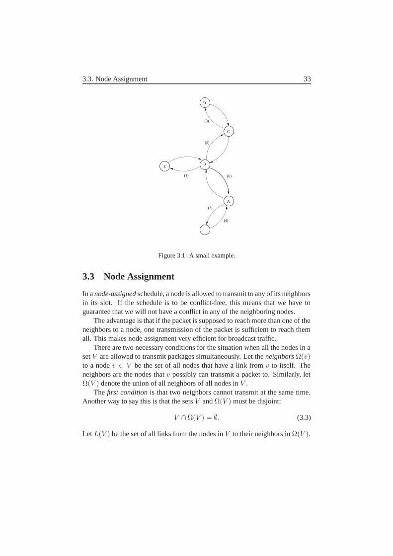
Figure 3.1 shows a small network. Assuming that interference betweennodes without communication links is small, we can see that links 1, 2 and 3can transmit simultaneously.
One problem with this assignment method is that it does not take advan-tage of the inherent broadcast properties of the radio medium. Each transmittedpacket will only be received by the assigned receiver despite being sent in alldirections (omnidirectional antennas). This is no problem with unicast traffic,but for broadcast traffic, where each packet should reach several destinations, itis inefficient. In these cases the packet has to be retransmitted for each of thesereceivers.
For example, if a broadcast packet has node B as source, it must be trans-mitted three times from node B. Link 1, 5 and 6 must transmit the packet atdifferent time slots. Then to reach the last destination, the packet must be trans-mitted on links 2 and 3. As these two links can transmit simultaneously, it ispossible to use only four time slots in order to reach all destinations.
3.3. Node Assignment 33
(1)
B
(3)
D
C
A
(2)
(4)
(6)
E
(5)
Figure 3.1: A small example.
3.3 Node Assignment
In a node-assigned schedule, a node is allowed to transmit to any of its neighborsin its slot. If the schedule is to be conflict-free, this means that we have toguarantee that we will not have a conflict in any of the neighboring nodes.
The advantage is that if the packet is supposed to reach more than one of theneighbors to a node, one transmission of the packet is sufficient to reach themall. This makes node assignment very efficient for broadcast traffic.
There are two necessary conditions for the situation when all the nodes in aset V are allowed to transmit packages simultaneously. Let the neighbors Ω(v)to a node v ∈ V be the set of all nodes that have a link from v to itself. Theneighbors are the nodes that v possibly can transmit a packet to. Similarly, letΩ(V ) denote the union of all neighbors of all nodes in V .
The first condition is that two neighbors cannot transmit at the same time.Another way to say this is that the sets V and Ω(V ) must be disjoint:
V ∩ Ω(V ) = ∅. (3.3)
Let L(V ) be the set of all links from the nodes in V to their neighbors in Ω(V ).
34 Chapter 3. Node and Link Assignment
Since it must be possible to use all the links in L(V ) for transmission simulta-neously, we state the second condition:
ΠL(V )(i, j) ≥ γR for all (i, j) ∈ L(V ) . (3.4)
If the above two conditions, (3.3) and (3.4), hold for a set of nodes V ∈ V ,we say that the set of nodes can transmit simultaneously.
If we return to the example network and compare it with link assignment,we see that the transmitting nodes to the three links that could transmit simulta-neously cannot be permitted to transmit simultaneously when we use the node-assignment strategy, since both node A and C may choose to transmit to B.
In the broadcast traffic example, nodes A, C and E can be reached by onetransmission of B, thereby decreasing the number of necessary transmissions.However, to reach the last two nodes we must transmit on A and C, and thesenodes cannot transmit simultaneously. This results in the use of three time slotsin order to reach all destinations, which is one time slot lower than for linkassignment.
3.4 Analysis
In this section we present some analytical results that are useful when evaluatingthe properties of node and link assignment. We first discuss maximum through-put and then continue with an approximation of the network delay at low trafficarrival rate.
In [66] the maximum throughput in a network with fixed capacities on thelinks and fixed routing is determined. Here, we will do the same specifically fora link-assigned schedule and a node-assigned schedule.
A link-assigned schedule contains, for each time slot in the frame, the setof links (i, j) that are allowed to transmit in that time slot. A node-assignedschedule contains the set of nodes vi that are allowed to transmit in each timeslot. We assume that the number of time slots in a frame, T . We do not considerpacket failures and retransmissions.
Each link may be assigned several time slots per frame. Let hij(SL) denotethe number of slots in schedule SL where link (i, j) can access a time slot andsimilarly let hi(SN) denote the number of slots in schedule SN where node vi
can access a time slot.
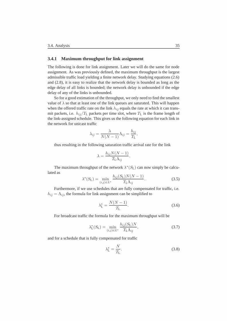
3.4. Analysis 35
3.4.1 Maximum throughput for link assignment
The following is done for link assignment. Later we will do the same for nodeassignment. As was previously defined, the maximum throughput is the largestadmissible traffic load yielding a finite network delay. Studying equations (2.6)and (2.8), it is easy to realize that the network delay is bounded as long as theedge delay of all links is bounded; the network delay is unbounded if the edgedelay of any of the links is unbounded.
So for a good estimation of the throughput, we only need to find the smallestvalue of λ so that at least one of the link queues are saturated. This will happenwhen the offered traffic rate on the link λij equals the rate at which it can trans-mit packets, i.e. hij/TL packets per time slot, where TL is the frame length ofthe link-assigned schedule. This gives us the following equation for each link inthe network for unicast traffic
λij =λ
N(N − 1)Λij =
hij
TL,
thus resulting in the following saturation traffic arrival rate for the link
λ =hijN(N − 1)
TLΛij.
The maximum throughput of the network λ∗(SL) can now simply be calcu-lated as
λ∗(SL) = min(i,j)∈L∗
hij(SL)N(N − 1)TLΛij
. (3.5)
Furthermore, if we use schedules that are fully compensated for traffic, i.e.hij = Λij , the formula for link assignment can be simplified to
λ∗L =
N(N − 1)TL
. (3.6)
For broadcast traffic the formula for the maximum throughput will be
λ∗L(SL) = min
(i,j)∈L∗
hij(SL)NTLΛij
, (3.7)
and for a schedule that is fully compensated for traffic
λ∗L =
N
TL. (3.8)
36 Chapter 3. Node and Link Assignment
0.2 0.3 0.4 0.5 0.6 0.7 0.8 0.9 10.99
0.992
0.994
0.996
0.998
1
1.002
1.004
1.006
1.008
1.01
Connectivity
λ sim
ulat
ed /
λ estim
ated
Figure 3.2: The figure shows the ratio between estimated values of the maximumthroughput and simulated values for the maximum throughput for networksof different connectivity. The ratio is plotted for 400 networks of size 10nodes with unicast traffic.
In Figure 3.2 we show a comparison of this estimation with simulation re-sults. As can be seen this estimation is sufficiently good for our purposes. Thelargest part of the deviation between simulated and estimated results is probablydue to the high delay variance of the simulation results close to the maximumthroughput, see Appendix A for more information.
3.4.2 Maximum throughput in node assignment
The corresponding notation for node assignment is hi(SN) as the number of timeslots assigned to node vi, and TN as the frame length. The maximum throughputfor node assignment in the case of unicast traffic is
λ∗(SN) = min(i∈V )
hi(SN)N(N − 1)TNΛi
, (3.9)
and the corresponding result for broadcast traffic can be written as
λ∗(SN) = min(i∈V )
Nhi(SN)TNΛi
. (3.10)
For schedules that are fully compensated for traffic, i.e. hi = Λi the formula
3.4. Analysis 37
for node assignment with unicast traffic can be simplified to
λ∗N =
N(N − 1)TN
(3.11)
and, similarly, for broadcast traffic
λ∗N =
N
TN. (3.12)
The ratio between the maximum throughput of a link-assigned schedule andthe maximum throughput of a node-assigned schedule can then be written as:
λ∗L
λ∗N
=TL
TN. (3.13)
Notice, this is valid for both unicast and broadcast traffic.
3.4.3 An approximative formula for the network delay
We now derive an expression for the network delay DL for a link-assignedschedule with unicast traffic,
DL =∑
(i,j)∈L
Λij
N(N − 1)dij , (3.14)
where dij is the average expected edge delay on link (i, j).In order to determine the network delay, we make two extra assumptions.
Even if they are not fulfilled, it is still a useful approximation of the networkdelay.
First, the slots in the schedules assigned to a node are perfectly spread overthe frame, i.e. the distance between two assigned slots is equal. The algorithmused in the simulations attempts to do this, but the algorithm is not optimal andit is not always possible to spread the slots evenly.
Second, the relay traffic can be described as a Poisson process. This iscertainly not the case, since relay packets can only arrive in specific time slots.However, it is normally a good approximation. This is an attempt to use thesame principle as the independence assumption [66], but for a TDMA networkwith fixed packet size.
38 Chapter 3. Node and Link Assignment
With these assumptions, the average expected edge delay for a link can atlow traffic arrival rate be written as:
dij =TL
2hij,
which inserted in (3.14) gives the network delay of a link-assigned schedule
DL =∑
(i,j)∈L
Λij
N(N − 1)TL
2hij.
Furthermore, if the schedule is fully compensated for traffic, we have
DL =MTL
2N(N − 1),
where M is the number of links in the network.The corresponding result for a node-assigned schedule is
DN =∑
i∈V
Λi
N(N − 1)TN
2hi,
and for a schedule fully compensated for traffic
DN =NTN
2N(N − 1).
The ratio between the network delay of link assignment and the networkdelay of node assignment can then be written as:
DL
DN=
M
N
TL
TN=
M
N
λ∗N
λ∗L. (3.15)
Simulations in the next section will show that this is a good approximationexcept for low connectivity.
3.5 Evaluation and Results
In this section we compare the delays and maximum throughput for node as-signment and link assignment. The results for network delay are generated bynetwork simulation as described in appendix A. Furthermore, for unicast traf-fic we compare these simulated results with the approximative results given insection 3.4. The comparison begins with unicast and concludes with broadcasttraffic.
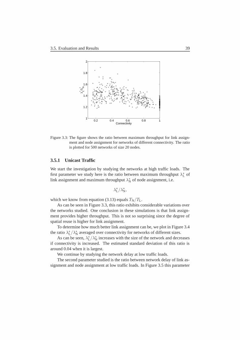
3.5. Evaluation and Results 39
0.2 0.4 0.6 0.8 11
1.2
1.4
1.6
1.8
2
Connectivity
λ* L/λ* N
Figure 3.3: The figure shows the ratio between maximum throughput for link assign-ment and node assignment for networks of different connectivity. The ratiois plotted for 500 networks of size 20 nodes.
3.5.1 Unicast Traffic
We start the investigation by studying the networks at high traffic loads. Thefirst parameter we study here is the ratio between maximum throughput λ∗
L oflink assignment and maximum throughput λ∗
N of node assignment, i.e.
λ∗L/λ∗
N,
which we know from equation (3.13) equals TN/TL.As can be seen in Figure 3.3, this ratio exhibits considerable variations over
the networks studied. One conclusion in these simulations is that link assign-ment provides higher throughput. This is not so surprising since the degree ofspatial reuse is higher for link assignment.
To determine how much better link assignment can be, we plot in Figure 3.4the ratio λ∗
L/λ∗N averaged over connectivity for networks of different sizes.
As can be seen, λ∗L/λ∗
N increases with the size of the network and decreasesif connectivity is increased. The estimated standard deviation of this ratio isaround 0.04 when it is largest.
We continue by studying the network delay at low traffic loads.The second parameter studied is the ratio between network delay of link as-
signment and node assignment at low traffic loads. In Figure 3.5 this parameter
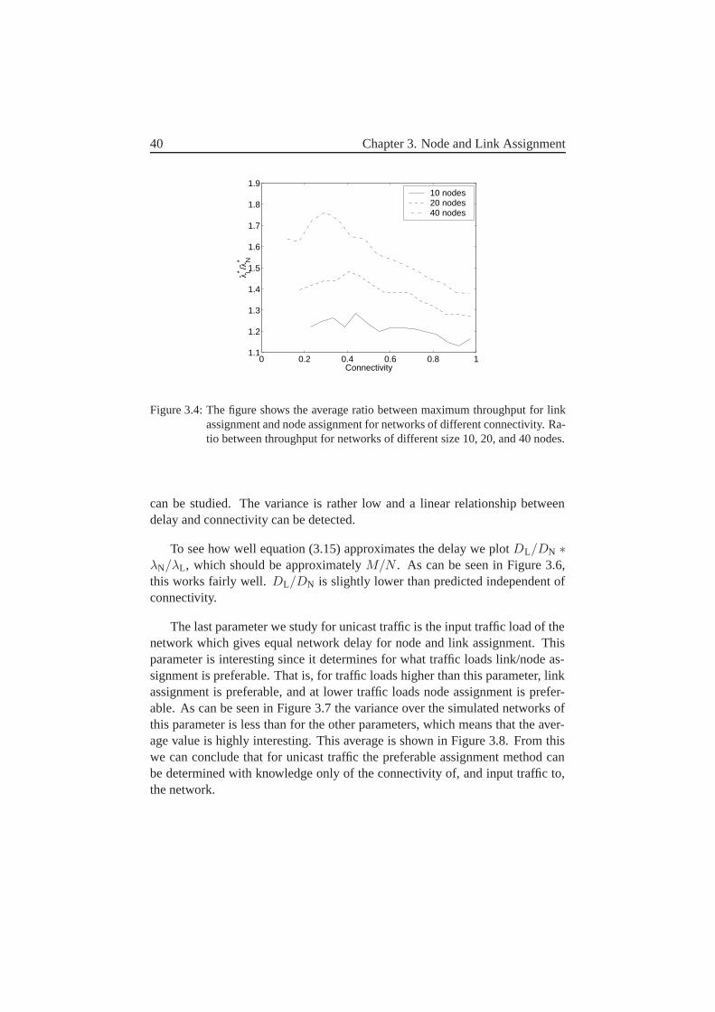
40 Chapter 3. Node and Link Assignment
0 0.2 0.4 0.6 0.8 11.1
1.2
1.3
1.4
1.5
1.6
1.7
1.8
1.9
Connectivity
λ* L/λ* N
10 nodes20 nodes40 nodes
Figure 3.4: The figure shows the average ratio between maximum throughput for linkassignment and node assignment for networks of different connectivity. Ra-tio between throughput for networks of different size 10, 20, and 40 nodes.
can be studied. The variance is rather low and a linear relationship betweendelay and connectivity can be detected.
To see how well equation (3.15) approximates the delay we plot DL/DN ∗λN/λL, which should be approximately M/N . As can be seen in Figure 3.6,this works fairly well. DL/DN is slightly lower than predicted independent ofconnectivity.
The last parameter we study for unicast traffic is the input traffic load of thenetwork which gives equal network delay for node and link assignment. Thisparameter is interesting since it determines for what traffic loads link/node as-signment is preferable. That is, for traffic loads higher than this parameter, linkassignment is preferable, and at lower traffic loads node assignment is prefer-able. As can be seen in Figure 3.7 the variance over the simulated networks ofthis parameter is less than for the other parameters, which means that the aver-age value is highly interesting. This average is shown in Figure 3.8. From thiswe can conclude that for unicast traffic the preferable assignment method canbe determined with knowledge only of the connectivity of, and input traffic to,the network.
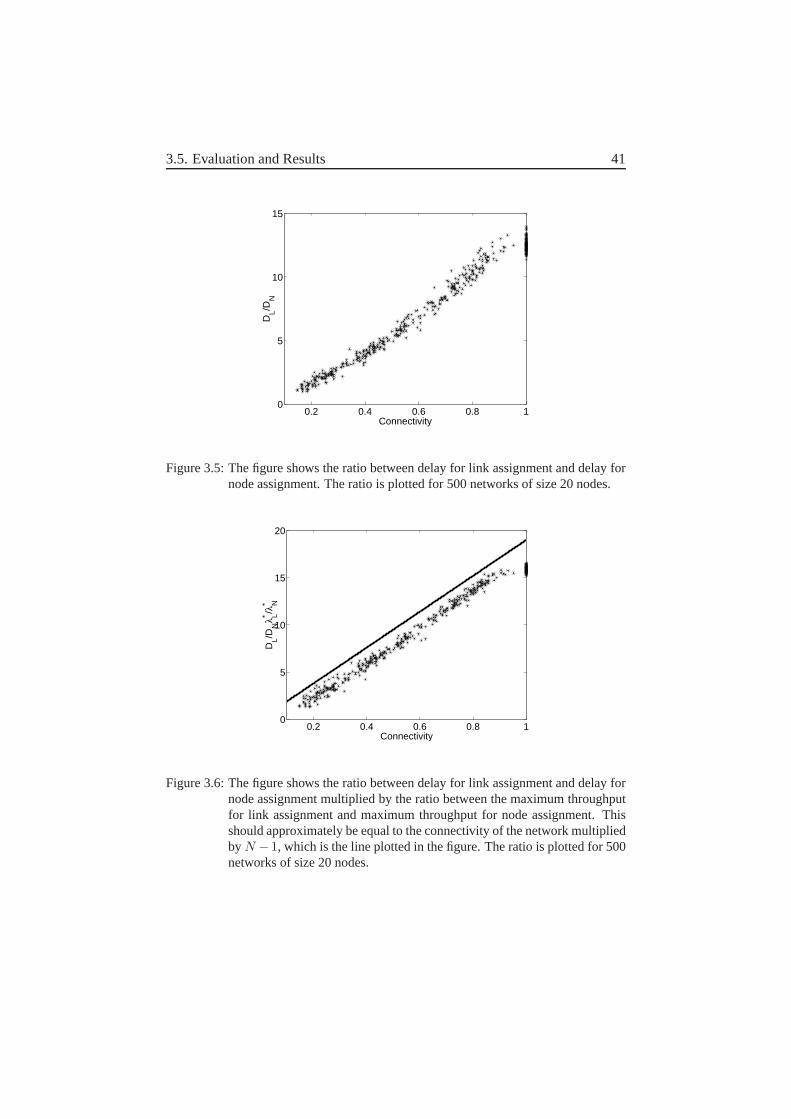
3.5. Evaluation and Results 41
0.2 0.4 0.6 0.8 10
5
10
15
Connectivity
DL/D
N
Figure 3.5: The figure shows the ratio between delay for link assignment and delay fornode assignment. The ratio is plotted for 500 networks of size 20 nodes.
0.2 0.4 0.6 0.8 10
5
10
15
20
Connectivity
DL/D
Nλ* L/λ
* N
Figure 3.6: The figure shows the ratio between delay for link assignment and delay fornode assignment multiplied by the ratio between the maximum throughputfor link assignment and maximum throughput for node assignment. Thisshould approximately be equal to the connectivity of the network multipliedby N − 1, which is the line plotted in the figure. The ratio is plotted for 500networks of size 20 nodes.
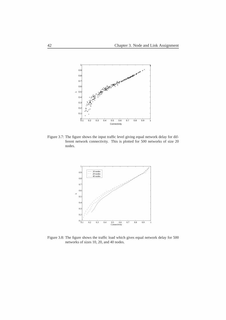
42 Chapter 3. Node and Link Assignment
0.1 0.2 0.3 0.4 0.5 0.6 0.7 0.8 0.9 10
0.1
0.2
0.3
0.4
0.5
0.6
0.7
0.8
0.9
1
Connectivity
λ
Figure 3.7: The figure shows the input traffic level giving equal network delay for dif-ferent network connectivity. This is plotted for 500 networks of size 20nodes.
0.1 0.2 0.3 0.4 0.5 0.6 0.7 0.8 0.9 10.1
0.2
0.3
0.4
0.5
0.6
0.7
0.8
0.9
1
Connectivity
λ
10 nodes20 nodes40 nodes
Figure 3.8: The figure shows the traffic load which gives equal network delay for 500networks of sizes 10, 20, and 40 nodes.
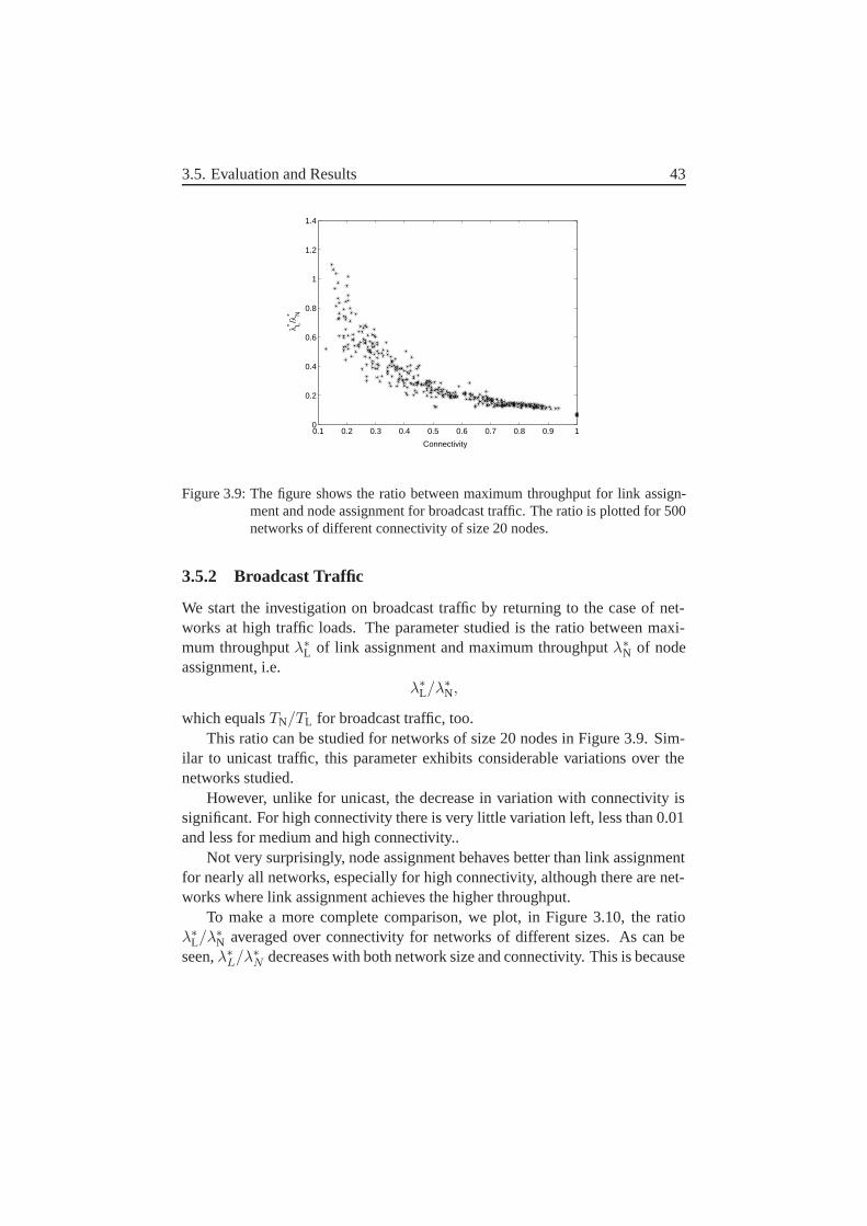
3.5. Evaluation and Results 43
0.1 0.2 0.3 0.4 0.5 0.6 0.7 0.8 0.9 10
0.2
0.4
0.6
0.8
1
1.2
1.4
Connectivity
λ* L/λ* N
Figure 3.9: The figure shows the ratio between maximum throughput for link assign-ment and node assignment for broadcast traffic. The ratio is plotted for 500networks of different connectivity of size 20 nodes.
3.5.2 Broadcast Traffic
We start the investigation on broadcast traffic by returning to the case of net-works at high traffic loads. The parameter studied is the ratio between maxi-mum throughput λ∗
L of link assignment and maximum throughput λ∗N of node
assignment, i.e.λ∗
L/λ∗N,
which equals TN/TL for broadcast traffic, too.This ratio can be studied for networks of size 20 nodes in Figure 3.9. Sim-
ilar to unicast traffic, this parameter exhibits considerable variations over thenetworks studied.
However, unlike for unicast, the decrease in variation with connectivity issignificant. For high connectivity there is very little variation left, less than 0.01and less for medium and high connectivity..
Not very surprisingly, node assignment behaves better than link assignmentfor nearly all networks, especially for high connectivity, although there are net-works where link assignment achieves the higher throughput.
To make a more complete comparison, we plot, in Figure 3.10, the ratioλ∗
L/λ∗N averaged over connectivity for networks of different sizes. As can be
seen, λ∗L/λ∗
N decreases with both network size and connectivity. This is because
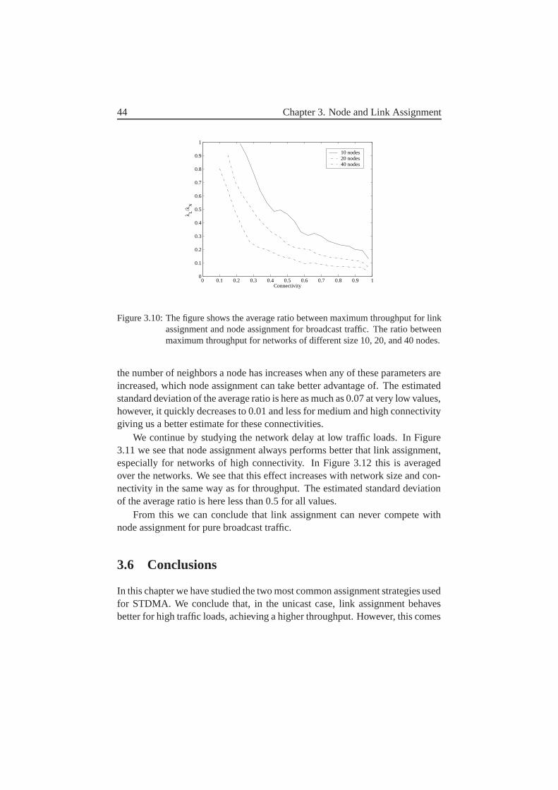
44 Chapter 3. Node and Link Assignment
0 0.1 0.2 0.3 0.4 0.5 0.6 0.7 0.8 0.9 10
0.1
0.2
0.3
0.4
0.5
0.6
0.7
0.8
0.9
1
Connectivity
λ L/λ
N
10 nodes20 nodes40 nodes
Figure 3.10: The figure shows the average ratio between maximum throughput for linkassignment and node assignment for broadcast traffic. The ratio betweenmaximum throughput for networks of different size 10, 20, and 40 nodes.
the number of neighbors a node has increases when any of these parameters areincreased, which node assignment can take better advantage of. The estimatedstandard deviation of the average ratio is here as much as 0.07 at very low values,however, it quickly decreases to 0.01 and less for medium and high connectivitygiving us a better estimate for these connectivities.
We continue by studying the network delay at low traffic loads. In Figure3.11 we see that node assignment always performs better that link assignment,especially for networks of high connectivity. In Figure 3.12 this is averagedover the networks. We see that this effect increases with network size and con-nectivity in the same way as for throughput. The estimated standard deviationof the average ratio is here less than 0.5 for all values.
From this we can conclude that link assignment can never compete withnode assignment for pure broadcast traffic.
3.6 Conclusions
In this chapter we have studied the two most common assignment strategies usedfor STDMA. We conclude that, in the unicast case, link assignment behavesbetter for high traffic loads, achieving a higher throughput. However, this comes
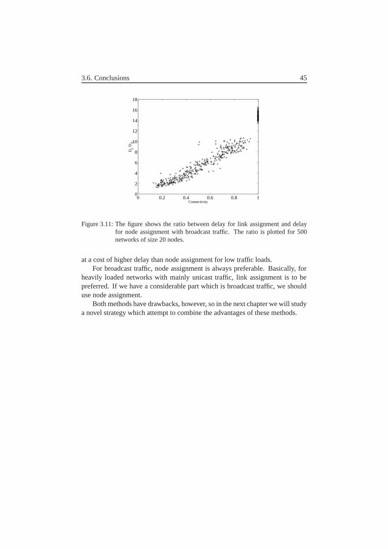
3.6. Conclusions 45
0 0.2 0.4 0.6 0.8 10
2
4
6
8
10
12
14
16
18
Connectivity
DL/D
N
Figure 3.11: The figure shows the ratio between delay for link assignment and delayfor node assignment with broadcast traffic. The ratio is plotted for 500networks of size 20 nodes.
at a cost of higher delay than node assignment for low traffic loads.For broadcast traffic, node assignment is always preferable. Basically, for
heavily loaded networks with mainly unicast traffic, link assignment is to bepreferred. If we have a considerable part which is broadcast traffic, we shoulduse node assignment.
Both methods have drawbacks, however, so in the next chapter we will studya novel strategy which attempt to combine the advantages of these methods.
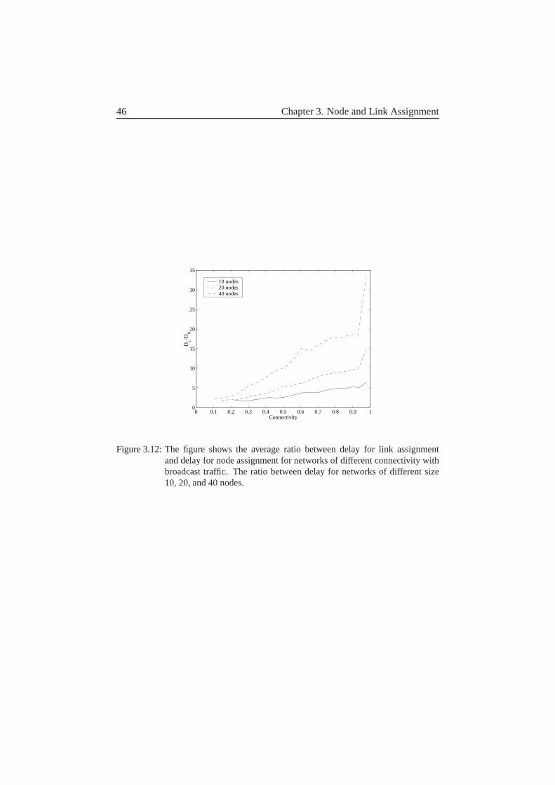
46 Chapter 3. Node and Link Assignment
0 0.1 0.2 0.3 0.4 0.5 0.6 0.7 0.8 0.9 10
5
10
15
20
25
30
35
Connectivity
DL/D
N
10 nodes20 nodes40 nodes
Figure 3.12: The figure shows the average ratio between delay for link assignmentand delay for node assignment for networks of different connectivity withbroadcast traffic. The ratio between delay for networks of different size10, 20, and 40 nodes.
Chapter 4
Extended Transmission Rights
In this chapter we present a novel assignment strategy which is based on linkassignment.
4.1 LET principle
Notice that the interference term in (2.3) depends only on which nodes that aretransmitting and not on the nodes that are receiving packets. Assume that a nodeis assigned as a transmitter in a slot, i.e. an outgoing link of the node is assignedthe slot. If this node redirects the transmission to a node, other than the assignedreceiving node, the inequality in (3.2) still holds for all links originally assignedto the slot. This means that the interference level of the other simultaneouslyreceiving nodes will not change. (Recall the assumption of omnidirectionalantennas.) The redirected transmission in itself cannot always be guaranteed tobe conflict-free.
Based on these observations, we suggest the following scheme for extend-ing transmission rights for any given link-assigned schedule. When a link isassigned a time slot, the node first checks whether there is a packet to transmiton that link. If there is no such packet, any other link with the same transmittingnode might be used if the node has a packet to transmit. Preferably links thatare conflict-free should have priority, so as to avoid unnecessary packet loss.
We call this strategy Link assignment with Extended Transmission rights(LET).
To illustrate how it works we present a simple example. Assume links 1,2, and 3 in Figure 4.1 have be scheduled to transmit in the same slot. Let us
47
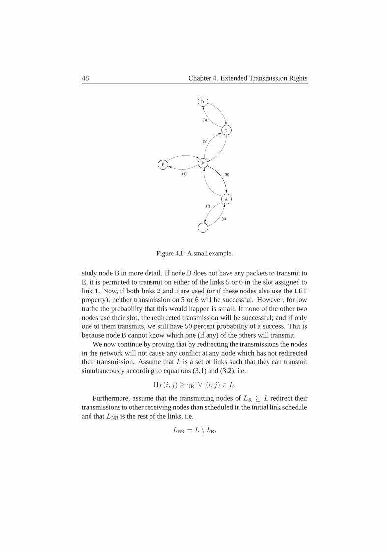
48 Chapter 4. Extended Transmission Rights
(1)
B
(3)
D
C
A
(2)
(4)
(6)
E
(5)
Figure 4.1: A small example.
study node B in more detail. If node B does not have any packets to transmit toE, it is permitted to transmit on either of the links 5 or 6 in the slot assigned tolink 1. Now, if both links 2 and 3 are used (or if these nodes also use the LETproperty), neither transmission on 5 or 6 will be successful. However, for lowtraffic the probability that this would happen is small. If none of the other twonodes use their slot, the redirected transmission will be successful; and if onlyone of them transmits, we still have 50 percent probability of a success. This isbecause node B cannot know which one (if any) of the others will transmit.
We now continue by proving that by redirecting the transmissions the nodesin the network will not cause any conflict at any node which has not redirectedtheir transmission. Assume that L is a set of links such that they can transmitsimultaneously according to equations (3.1) and (3.2), i.e.
ΠL(i, j) ≥ γR ∀ (i, j) ∈ L.
Furthermore, assume that the transmitting nodes of LR ⊆ L redirect theirtransmissions to other receiving nodes than scheduled in the initial link scheduleand that LNR is the rest of the links, i.e.
LNR = L \ LR.
4.1. LET principle 49
Let LU be the set of links used by the redirecting nodes, therefore,
VT(LU) = VT(LR).
If LNR is to be conflict-free, the following inequality must be valid
ΠLNR∪LU(i, j) ≥ γ1 ∀ (i, j) ∈ LNR.
For any (i, j) ∈ LNR, we can write
ΠLNR∪LU(i, j) =PiG(i, j)
(Nr + ILNR∪LU(i, j)).
and
ILNR∪LU(i, j) =∑
vk∈VT(LNR∪LU)\vi
Pk
Lb(k, j).
However,
VT(LNR ∪ LU) = VT(LNR) ∪ VT(LU) = VT(LNR) ∪ VT(LR) = VT(L),
resulting in, ILNR∪LU(i, j) = IL(i, j) and ΠLNR∪LU(i, j) = ΠL(i, j), which ofcourse fulfills (3.2).
For broadcast traffic, the situation will be a little more complicated. Eachpacket transmitted may have more than one receiver. This means that some, butnot all, packets may be received correctly. A worst case scenario would be thatonly transmissions over scheduled links would be received, and all of the rest ofthe links must be retransmitted. LET can then behave exactly as link assignmentfor high traffic loads. On the other hand, for low traffic loads, the behavior willbe that of node assignment, due to the low interference in the network. (Theinterference may be higher for broadcast traffic than for unicast traffic since apacket will be split and then might be relayed simultaneously by two nodes.)
However, there is also a possibility that more links than scheduled happento be collision-free. This can easily be the case if two nodes lie close each other.Any transmission with sufficiently high SIR to one of them will also reach theother with sufficiently high SIR.
The variable distance between the nodes in this type of network would beanother reason for an improvement compared to link assignment. If the distancebetween transmitter and receiver is small enough, the signal strength will besufficient to handle very high interference, which can often be the case even ifthe link is not scheduled to the time slot.
50 Chapter 4. Extended Transmission Rights
We conclude this section by giving a more formal description of the LETalgorithm that we use in our simulations.
This is done in each node:
Step 1 If there is a packet in the scheduled link’s queue:
1.1 Transmit this packet on all links that it is supposed to be transmittedon.
1.2 Remove the packet from all link queues where this transmission wassuccessful.
Step 2 Otherwise if there is no such packet. Choose one of the node’s otheroutgoing links that can be exchanged conflict-free in the schedule thathas a packet in queue:
2.1 Transmit this packet on all links that it is supposed to be transmittedon.
2.2 Remove the packet from all link queues where this transmission wassuccessful.
Step 3 Otherwise if there is no such packet. Choose one of the rest of the node’soutgoing links that has a packet in queue:
3.1 Transmit this packet on all links that it is supposed to be transmittedon.
3.2 Remove the packet from all link queues where this transmission wassuccessful.
Step 4 Otherwise, do nothing.
4.2 Basic Properties
In Figure 4.2, network delay for different λ is shown schedules using for threedifferent assignment strategies in a network of 30 nodes with unicast traffic. Theassignment strategies are node assignment, link assignment and LET.
We see from this figure that in this network, link assignment is preferable tonode assignment for high traffic loads. For low traffic loads, node assignmentachieves a smaller delay. The LET method combines the advantages of the twomethods and in this case achieves a smaller delay for all traffic loads.
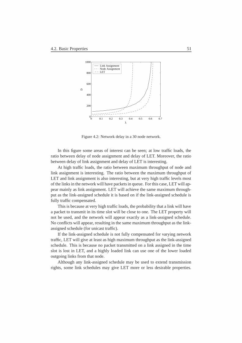
4.2. Basic Properties 51
0 0.1 0.2 0.3 0.4 0.5 0.6 0.70
200
400
600
800
1000
λ
D
Link AssignmentNode AssignmentLET
Figure 4.2: Network delay in a 30 node network.
In this figure some areas of interest can be seen; at low traffic loads, theratio between delay of node assignment and delay of LET. Moreover, the ratiobetween delay of link assignment and delay of LET is interesting.
At high traffic loads, the ratio between maximum throughput of node andlink assignment is interesting. The ratio between the maximum throughput ofLET and link assignment is also interesting, but at very high traffic levels mostof the links in the network will have packets in queue. For this case, LET will ap-pear mainly as link assignment. LET will achieve the same maximum through-put as the link-assigned schedule it is based on if the link-assigned schedule isfully traffic compensated.
This is because at very high traffic loads, the probability that a link will havea packet to transmit in its time slot will be close to one. The LET property willnot be used, and the network will appear exactly as a link-assigned schedule.No conflicts will appear, resulting in the same maximum throughput as the link-assigned schedule (for unicast traffic).
If the link-assigned schedule is not fully compensated for varying networktraffic, LET will give at least as high maximum throughput as the link-assignedschedule. This is because no packet transmitted on a link assigned in the timeslot is lost in LET, and a highly loaded link can use one of the lower loadedoutgoing links from that node.
Although any link-assigned schedule may be used to extend transmissionrights, some link schedules may give LET more or less desirable properties.
52 Chapter 4. Extended Transmission Rights
Here we discuss what effect the link schedule has on delay.At low traffic load, the nodes will normally only have at most one packet in
queue at a time. In this case, LET behaves as node assignment, with the node-assigned schedule as the transmitting nodes in the link-assigned schedule. Aproblem when generating STDMA schedules is how to determine which slotsto give a node or link that is going to receive more than one slot, since delaythrough the node depends on which specific time slots the node is given.
For example, assume that a node has received two time slots and these arespread in such a way that the distance between them is approximately half theframe length. Then for low traffic loads, the delay will be at most half theframe length. If the node is given two consecutive time slots, the maximumdelay might be the entire frame length. That is, it is usually efficient to spreada node’s time slots evenly over the frame. This problem gets worse if nodesreceive many time slots, especially since a large part of the traffic usually flowsthrough these nodes.
In some algorithms, see e.g. [30], an effort is made to spread the timeslots a node or link is given equally over the frame. However, even if the linkschedule has perfectly spread time slots, this may not be the case for the trans-mitting nodes. Therefore, LET might give considerably higher delay than anode-assigned schedule if the link schedule tends to give the transmitting nodesconsecutive time slots.
Any assignment algorithm, especially if it is of a greedy type, has a set ofrules to determine which link to assign to a time slot. One method used is nodeID, i.e. the lower the ID number, the higher the priority. To assign links, thepair of node IDs of the transmitting and receiving nodes can be used. A sortedlist according to link priority would then give the outgoing links from a nodeconsecutive places in the list. Even if another system for link priority is used,node ID is probably eventually used if priority is equal for several links.
Now, assume we have a fully connected network, i.e. all nodes can com-municate with all other nodes without relaying. Furthermore, in this case wecan assume that there is no spatial reuse, although in a link schedule using aninterference-based model, this might be possible due to capture. In this case theassigned schedule would be the sorted list described above, which gives highnetwork delay.
One way to avoid this problem is to give the links a link ID which is random,although different, for each link.
The assumptions used in this paper is the use of omnidirectional antennasand equal transmission power of all nodes in the network. If this is not the case,
4.3. Analysis 53
a node cannot redirect its transmission to any other of its neighbors since thismight require an increase of signal power or redirection of the antennas. Anychange of the outgoing power strength and direction can ruin the conflict-freeproperties of the other receiving nodes.
However, some of the nodes may still be reached without such a change,and the LET properties can still be used with these nodes, although this is lessefficient than if all nodes could be reached.
An alternative way of designing a LET schedule would be to base it on anode-assigned schedule instead and replace each node in the schedule with oneof its outgoing links. Using LET on this schedule would result in a schedule thatwould behave as a node-assigned schedule for all traffic loads and traffic types,thereby achieving the advantages of node assignment for broadcast traffic. Theactual order in which packets are transmitted can be different, though.
Unfortunately, this schedule would not have the positive properties of linkassignment for unicast traffic.
4.3 Analysis
The same assumptions as we made for node and link assignment in previouschapter can be made for LET as well. However, since LET behaves like a node-assigned schedule at low traffic loads, the link-assigned schedule would have totry to spread the time slots for the transmitting nodes of the links evenly overthe frame instead of the link time slots. However, the algorithm used in thesimulations does not attempt to do this. This results in a larger discrepancy thanfor node assignment or link assignment when compared with simulations.
The network delay for unicast traffic using LET for low traffic loads underthese assumptions can be written as:
DLET =∑
i∈V
Λi
N(N − 1)TL
2hi. (4.1)
For a schedule fully compensated for unicast traffic hi = Λi, this results in,
DLET =NTL
2N(N − 1).
The ratio between network delay of link assignment and network delay ofLET for unicast traffic can be written as
DL
DLET=
M
N. (4.2)
54 Chapter 4. Extended Transmission Rights
and the ratio between network delay of node assignment and network delay ofLET can be written as
DN
DLET=
TN
TL=
λ∗L
λ∗N
. (4.3)
4.4 Evaluation and Results
In this section we compare the delays and maximum throughput for LET withnode assignment and link assignment. The results for network delay are gen-erated by network simulation. No comparison for maximum throughput inthe case of unicast traffic is included since LET achieves the same maximumthroughput as link assignment. For broadcast traffic such a comparison is in-cluded, using simulations to determine the maximum throughput for LET.
Furthermore, we compare these simulated results with the approximativeresults for unicast traffic given in section 4.3.
In the simulations of LET we have the extra simulation assumption that thelink ID is random, as described in section 4.2.
4.4.1 Unicast Traffic
The first comparison is node assignment and LET. Therefore, the parameterstudied is the ratio between network delay of node assignment and networkdelay of LET at low traffic loads, i.e.
DN/DLET.
If this parameter is greater than one, LET is always preferable. If it is less thanone, node assignment is preferable for low traffic loads.
In Figure 4.3, this parameter can be studied for networks of size 20 nodes.As can be seen there are some variations over the different networks. In Figure4.4 we plot the ratio DLET/DN averaged over connectivity for networks of dif-ferent sizes. As can be seen, DLET/DN decreases with the connectivity. This isbecause the gain in spatial reuse of link assignment compared with node assign-ment decreases with connectivity. Its increase with network size is consistentwith the approximation in equation (4.3), since it should be close to λL/λN. Butit should also be noted that the estimated standard deviation of the average ra-tio is on about the same order as the difference between the different networksizes. It is here on the order of 0.1 for the low values and less than 0.03 above aconnectivity of 0.4.
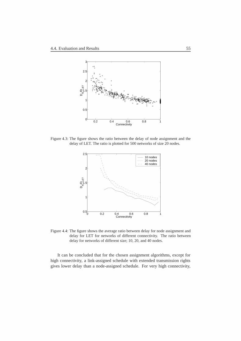
4.4. Evaluation and Results 55
0.2 0.4 0.6 0.8 10
0.5
1
1.5
2
2.5
3
Connectivity
DN
/DLE
T
Figure 4.3: The figure shows the ratio between the delay of node assignment and thedelay of LET. The ratio is plotted for 500 networks of size 20 nodes.
0 0.2 0.4 0.6 0.8 10.5
1
1.5
2
2.5
Connectivity
DN
/DLE
T
10 nodes20 nodes40 nodes
Figure 4.4: The figure shows the average ratio between delay for node assignment anddelay for LET for networks of different connectivity. The ratio betweendelay for networks of different size; 10, 20, and 40 nodes.
It can be concluded that for the chosen assignment algorithms, except forhigh connectivity, a link-assigned schedule with extended transmission rightsgives lower delay than a node-assigned schedule. For very high connectivity,
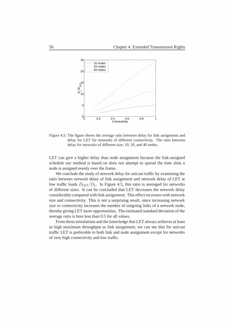
56 Chapter 4. Extended Transmission Rights
0 0.2 0.4 0.6 0.8 10
5
10
15
20
25
Connectivity
DL/D
LET
10 nodes20 nodes40 nodes
Figure 4.5: The figure shows the average ratio between delay for link assignment anddelay for LET for networks of different connectivity. The ratio betweendelay for networks of different size; 10, 20, and 40 nodes.
LET can give a higher delay than node assignment because the link-assignedschedule our method is based on does not attempt to spread the time slots anode is assigned evenly over the frame.
We conclude the study of network delay for unicast traffic by examining theratio between network delay of link assignment and network delay of LET atlow traffic loads DLET/DL. In Figure 4.5, this ratio is averaged for networksof different sizes. It can be concluded that LET decreases the network delayconsiderably compared with link assignment. This effect increases with networksize and connectivity. This is not a surprising result, since increasing networksize or connectivity increases the number of outgoing links of a network node,thereby giving LET more opportunities. The estimated standard deviation of theaverage ratio is here less than 0.5 for all values.
From these simulations and the knowledge that LET always achieves at leastas high maximum throughput as link assignment, we can see that for unicasttraffic LET is preferable to both link and node assignment except for networksof very high connectivity and low traffic.
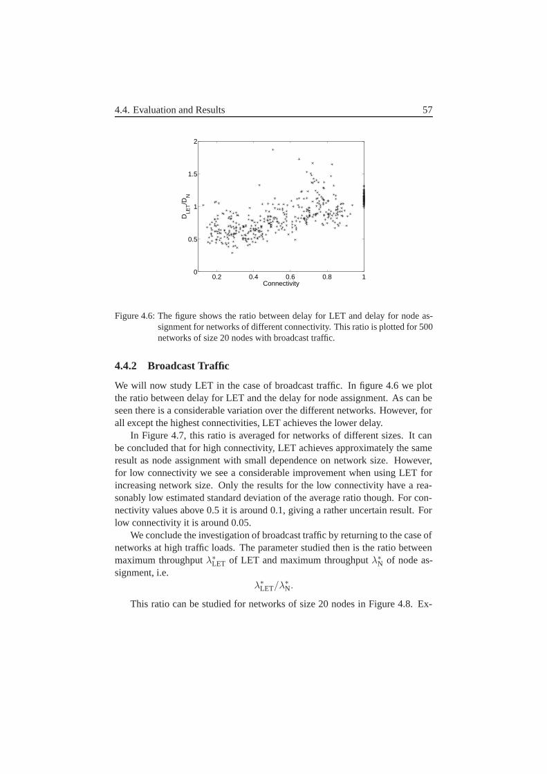
4.4. Evaluation and Results 57
0.2 0.4 0.6 0.8 10
0.5
1
1.5
2
Connectivity
DLE
T/D
N
Figure 4.6: The figure shows the ratio between delay for LET and delay for node as-signment for networks of different connectivity. This ratio is plotted for 500networks of size 20 nodes with broadcast traffic.
4.4.2 Broadcast Traffic
We will now study LET in the case of broadcast traffic. In figure 4.6 we plotthe ratio between delay for LET and the delay for node assignment. As can beseen there is a considerable variation over the different networks. However, forall except the highest connectivities, LET achieves the lower delay.
In Figure 4.7, this ratio is averaged for networks of different sizes. It canbe concluded that for high connectivity, LET achieves approximately the sameresult as node assignment with small dependence on network size. However,for low connectivity we see a considerable improvement when using LET forincreasing network size. Only the results for the low connectivity have a rea-sonably low estimated standard deviation of the average ratio though. For con-nectivity values above 0.5 it is around 0.1, giving a rather uncertain result. Forlow connectivity it is around 0.05.
We conclude the investigation of broadcast traffic by returning to the case ofnetworks at high traffic loads. The parameter studied then is the ratio betweenmaximum throughput λ∗
LET of LET and maximum throughput λ∗N of node as-
signment, i.e.λ∗
LET/λ∗N.
This ratio can be studied for networks of size 20 nodes in Figure 4.8. Ex-
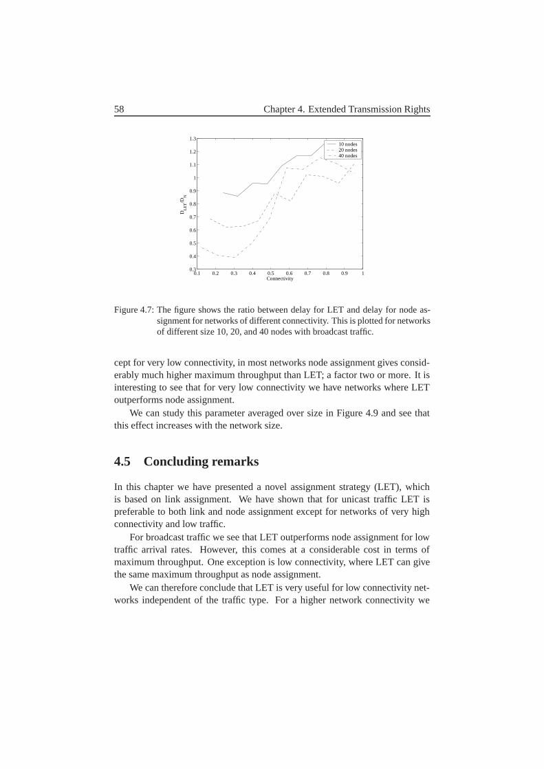
58 Chapter 4. Extended Transmission Rights
0.1 0.2 0.3 0.4 0.5 0.6 0.7 0.8 0.9 10.3
0.4
0.5
0.6
0.7
0.8
0.9
1
1.1
1.2
1.3
Connectivity
DL
ET/D
N
10 nodes20 nodes40 nodes
Figure 4.7: The figure shows the ratio between delay for LET and delay for node as-signment for networks of different connectivity. This is plotted for networksof different size 10, 20, and 40 nodes with broadcast traffic.
cept for very low connectivity, in most networks node assignment gives consid-erably much higher maximum throughput than LET; a factor two or more. It isinteresting to see that for very low connectivity we have networks where LEToutperforms node assignment.
We can study this parameter averaged over size in Figure 4.9 and see thatthis effect increases with the network size.
4.5 Concluding remarks
In this chapter we have presented a novel assignment strategy (LET), whichis based on link assignment. We have shown that for unicast traffic LET ispreferable to both link and node assignment except for networks of very highconnectivity and low traffic.
For broadcast traffic we see that LET outperforms node assignment for lowtraffic arrival rates. However, this comes at a considerable cost in terms ofmaximum throughput. One exception is low connectivity, where LET can givethe same maximum throughput as node assignment.
We can therefore conclude that LET is very useful for low connectivity net-works independent of the traffic type. For a higher network connectivity we
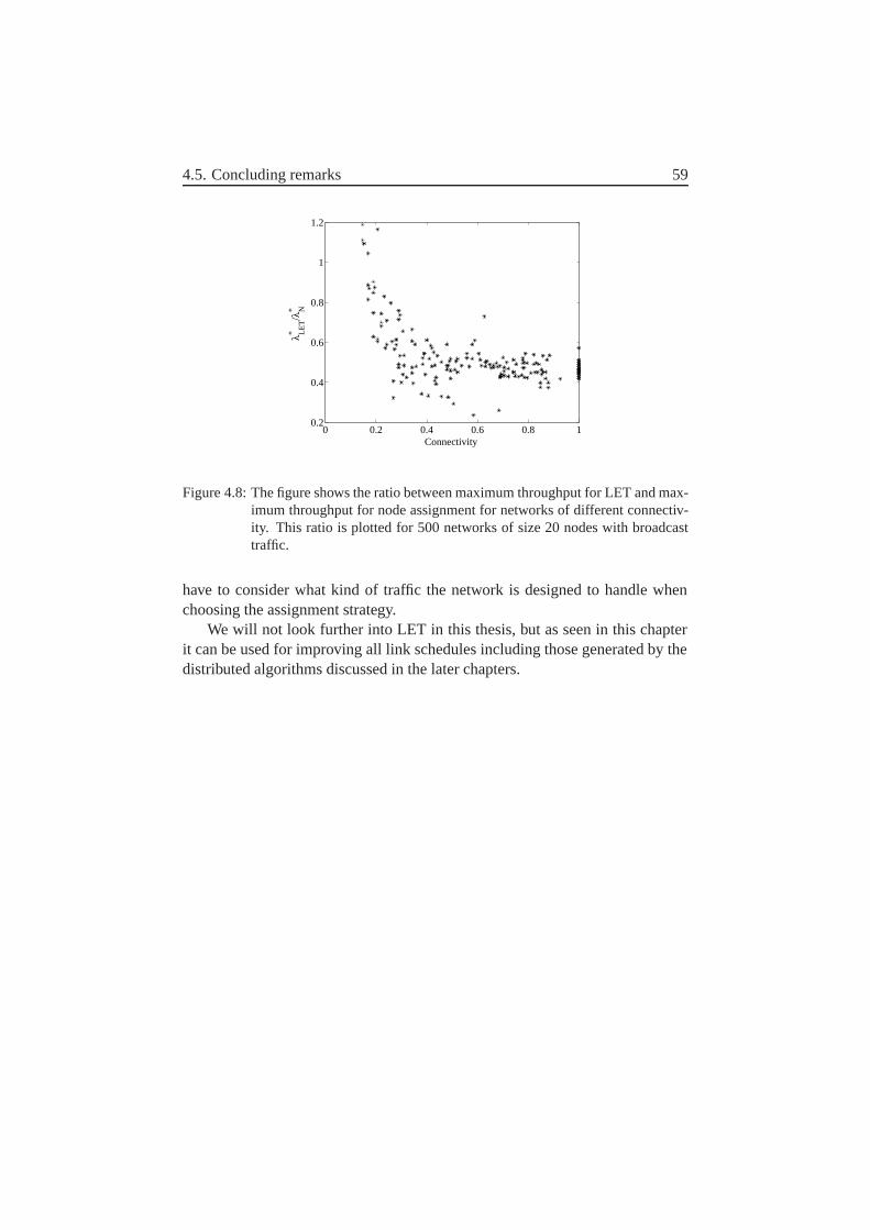
4.5. Concluding remarks 59
0 0.2 0.4 0.6 0.8 10.2
0.4
0.6
0.8
1
1.2
Connectivity
λ* LE
T/λ
* N
Figure 4.8: The figure shows the ratio between maximum throughput for LET and max-imum throughput for node assignment for networks of different connectiv-ity. This ratio is plotted for 500 networks of size 20 nodes with broadcasttraffic.
have to consider what kind of traffic the network is designed to handle whenchoosing the assignment strategy.
We will not look further into LET in this thesis, but as seen in this chapterit can be used for improving all link schedules including those generated by thedistributed algorithms discussed in the later chapters.
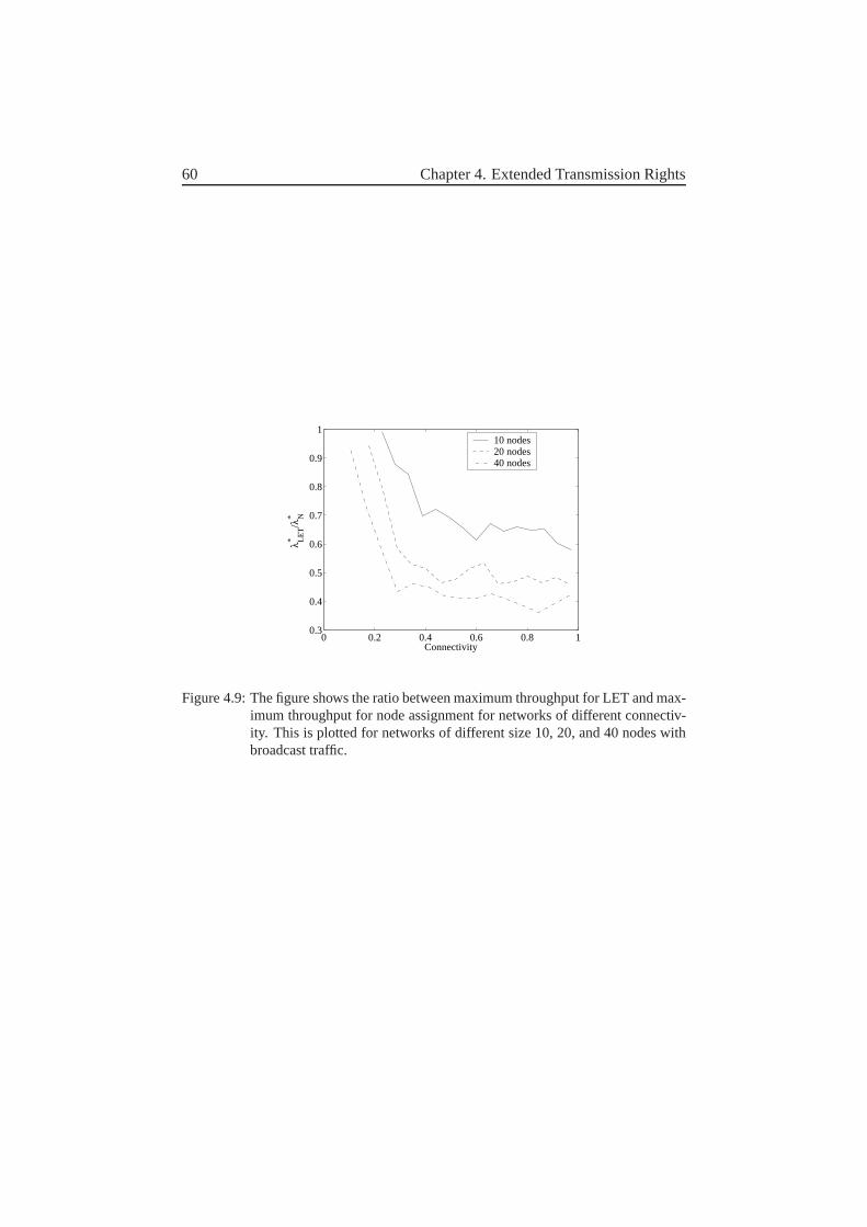
60 Chapter 4. Extended Transmission Rights
0 0.2 0.4 0.6 0.8 10.3
0.4
0.5
0.6
0.7
0.8
0.9
1
Connectivity
λ* LE
T/λ
* N
10 nodes20 nodes40 nodes
Figure 4.9: The figure shows the ratio between maximum throughput for LET and max-imum throughput for node assignment for networks of different connectiv-ity. This is plotted for networks of different size 10, 20, and 40 nodes withbroadcast traffic.
Chapter 5
Model Comparison
In this chapter we investigate the loss of capacity (in terms of throughput) whenthe STDMA algorithm has limited information about the network. We will stilluse a centralized algorithm to generate the schedules but limit the network infor-mation when we decide which links can transmit simultaneously. We will startby describing the traditional graph model and continue with more advancedmodels, with more information.
A somewhat different approach to solving this problem have been taken in[12]. In which they use a truncated graph model to give probabilistic guaranteesfor the maximum throughput by bounding the maximum number of simultane-ous transmitting units.
5.1 Graph-based Network Model
The traditional approach of designing reuse schedules is to use a graph modelof the network. A graph consists of a set of nodes and a set of edges connectingpairs of nodes. In a graph representation of a radio network, each radio terminalis represented by a node, and the set of edges represents the pair of nodes thatcan communicate directly, i.e. radio links. In the simplest form of schedulingit is assumed that the lack of an edge means that two nodes cannot affect eachother even as interferences. In such scheduling, a node can be assigned to sendin a time slot if it has no edge to a node assigned to receive, and a node can beassigned to receive if no node at one-hop distance is assigned to send.
This method can easily be expanded to distances at more that one hop. Forexample, one way to do this is to assume that all nodes at exactly two hops
61
62 Chapter 5. Model Comparison
distance are also creating too much interference for simultaneous transmission.This means that a node cannot be assigned to receive on a link in a time slot ifany node at distance one or two is scheduled to send (and the opposite).
This can be generalized to all nodes at k hops distance, and we will de-note the method as k-hop graph scheduling. This method has sometimes beenused in USAP [21]. The traditional way of scheduling will be the 1-hop graphscheduling.
By using a k larger than 1, we include most of the nodes that cause the mostinterference with the additional benefit that we do not have to determine exactlywhich nodes they are. A drawback of this method is that it may overestimate theinterference caused by neighbors further away, thereby causing fewer assignedtime slots than would otherwise be possible. We may also have interferencesnot considered from nodes further away than k hops.
In the graph-based method, a graph representation Gγ is chosen. To repre-sent the radio network as a directed graph, we denote by Gγ the directed graphthat is obtained by defining the set of nodes V as vertices and the set of edges Eas follows
(i, j) ∈ E if and only if Γij ≥ γ ,
i.e. the set of edges is the set of node pairs with SNR not smaller than γ.The schedule is then designed from the graph Gγ . Interferences from other
nodes are not taken into account. The traditional method for node assignmentgiven a set of edges is to say that two nodes vi and vj can use the same time slotif and only if:
• edge (i, j) /∈ E and edge (j, i) /∈ E, and
• there is no vk such that (j, k) ∈ E and (i, k) ∈ E
The first criterion is based on a node not being able to receive and transmit si-multaneously in the same slot. The second criterion is that a node cannot receivea packet from more than one node in the same slot. These criteria translate tothe condition that nodes must be at least two hops away from each other in orderto be scheduled to the same slot. For a more precise description of this problemsee [8].
Observe that the above criteria are not sufficient to guarantee that the assign-ment is conflict-free in terms of SIR, as defined in chapter 2. The assignmentsthat fulfill the above two criteria do not necessarily fulfill the SIR criterion givenin condition (3.2). They may therefore not be able to transmit simultaneously
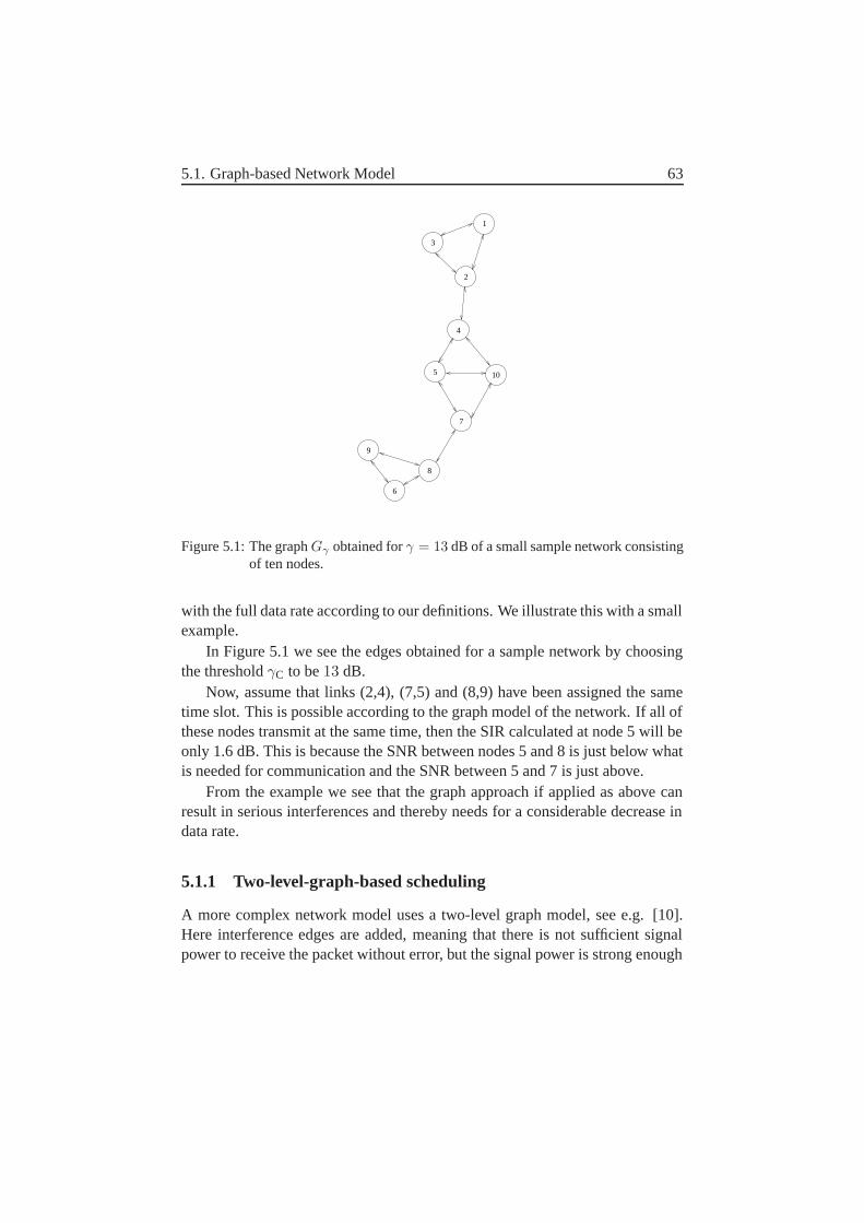
5.1. Graph-based Network Model 63
3
1
2
4
5 10
7
8
6
9
Figure 5.1: The graph Gγ obtained for γ = 13 dB of a small sample network consistingof ten nodes.
with the full data rate according to our definitions. We illustrate this with a smallexample.
In Figure 5.1 we see the edges obtained for a sample network by choosingthe threshold γC to be 13 dB.
Now, assume that links (2,4), (7,5) and (8,9) have been assigned the sametime slot. This is possible according to the graph model of the network. If all ofthese nodes transmit at the same time, then the SIR calculated at node 5 will beonly 1.6 dB. This is because the SNR between nodes 5 and 8 is just below whatis needed for communication and the SNR between 5 and 7 is just above.
From the example we see that the graph approach if applied as above canresult in serious interferences and thereby needs for a considerable decrease indata rate.
5.1.1 Two-level-graph-based scheduling
A more complex network model uses a two-level graph model, see e.g. [10].Here interference edges are added, meaning that there is not sufficient signalpower to receive the packet without error, but the signal power is strong enough
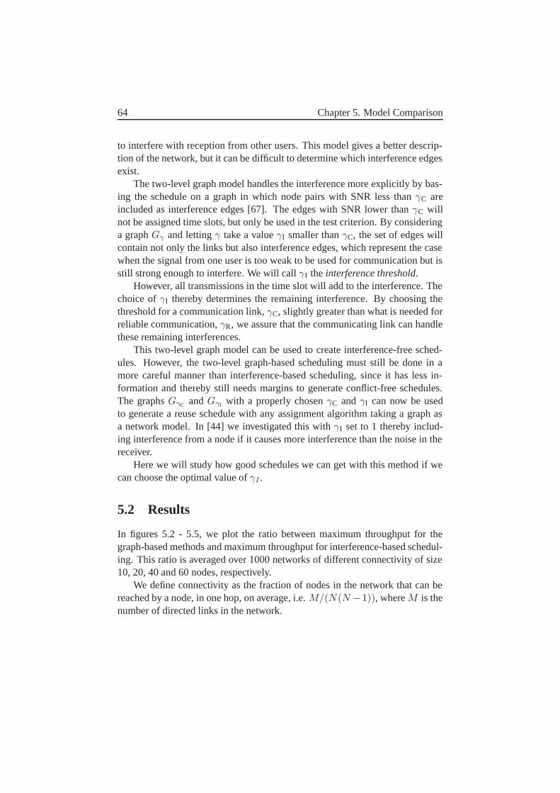
64 Chapter 5. Model Comparison
to interfere with reception from other users. This model gives a better descrip-tion of the network, but it can be difficult to determine which interference edgesexist.
The two-level graph model handles the interference more explicitly by bas-ing the schedule on a graph in which node pairs with SNR less than γC areincluded as interference edges [67]. The edges with SNR lower than γC willnot be assigned time slots, but only be used in the test criterion. By consideringa graph Gγ and letting γ take a value γI smaller than γC, the set of edges willcontain not only the links but also interference edges, which represent the casewhen the signal from one user is too weak to be used for communication but isstill strong enough to interfere. We will call γI the interference threshold.
However, all transmissions in the time slot will add to the interference. Thechoice of γI thereby determines the remaining interference. By choosing thethreshold for a communication link, γC, slightly greater than what is needed forreliable communication, γR, we assure that the communicating link can handlethese remaining interferences.
This two-level graph model can be used to create interference-free sched-ules. However, the two-level graph-based scheduling must still be done in amore careful manner than interference-based scheduling, since it has less in-formation and thereby still needs margins to generate conflict-free schedules.The graphs GγC and GγI with a properly chosen γC and γI can now be usedto generate a reuse schedule with any assignment algorithm taking a graph asa network model. In [44] we investigated this with γI set to 1 thereby includ-ing interference from a node if it causes more interference than the noise in thereceiver.
Here we will study how good schedules we can get with this method if wecan choose the optimal value of γI .
5.2 Results
In figures 5.2 - 5.5, we plot the ratio between maximum throughput for thegraph-based methods and maximum throughput for interference-based schedul-ing. This ratio is averaged over 1000 networks of different connectivity of size10, 20, 40 and 60 nodes, respectively.
We define connectivity as the fraction of nodes in the network that can bereached by a node, in one hop, on average, i.e. M/(N(N −1)), where M is thenumber of directed links in the network.
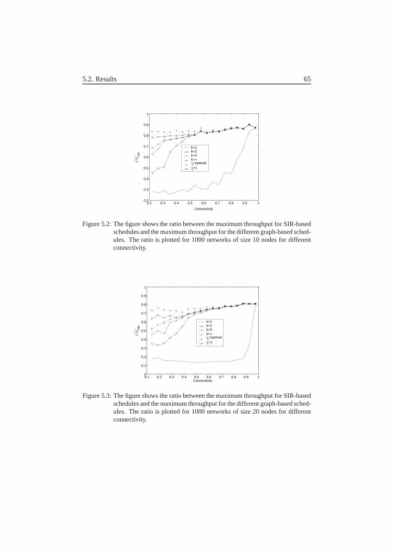
5.2. Results 65
0.2 0.3 0.4 0.5 0.6 0.7 0.8 0.9 10.2
0.3
0.4
0.5
0.6
0.7
0.8
0.9
1
Connectivity
λ* /λ* S
IR
k=1k=2k=3k=∞γI=optimal
γI=1
Figure 5.2: The figure shows the ratio between the maximum throughput for SIR-basedschedules and the maximum throughput for the different graph-based sched-ules. The ratio is plotted for 1000 networks of size 10 nodes for differentconnectivity.
0.1 0.2 0.3 0.4 0.5 0.6 0.7 0.8 0.9 10
0.1
0.2
0.3
0.4
0.5
0.6
0.7
0.8
0.9
1
Connectivity
λ* /λ* S
IR
k=1k=2k=3k=∞γI=optimal
γI=1
Figure 5.3: The figure shows the ratio between the maximum throughput for SIR-basedschedules and the maximum throughput for the different graph-based sched-ules. The ratio is plotted for 1000 networks of size 20 nodes for differentconnectivity.
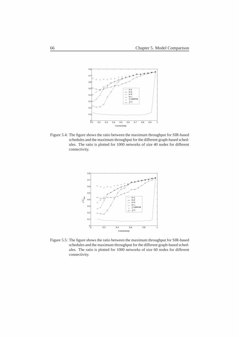
66 Chapter 5. Model Comparison
0.1 0.2 0.3 0.4 0.5 0.6 0.7 0.8 0.9 10
0.1
0.2
0.3
0.4
0.5
0.6
0.7
0.8
Connectivity
k=1k=2k=3k=∞γI=optimal
γI=1
Figure 5.4: The figure shows the ratio between the maximum throughput for SIR-basedschedules and the maximum throughput for the different graph-based sched-ules. The ratio is plotted for 1000 networks of size 40 nodes for differentconnectivity.
0 0.2 0.4 0.6 0.8 10
0.1
0.2
0.3
0.4
0.5
0.6
0.7
0.8
Connectivity
λ* /λ* S
IR k=1k=2k=3k=∞γI=optimal
γI=1
Figure 5.5: The figure shows the ratio between the maximum throughput for SIR-basedschedules and the maximum throughput for the different graph-based sched-ules. The ratio is plotted for 1000 networks of size 60 nodes for differentconnectivity.
5.3. Concluding remarks 67
It can be seen that the difference between all graph-based scheduling meth-ods and interference-based scheduling increases with networks size. Two-levelgraph based scheduling with an optimal choice of γI performs best of the graph-based methods especially for low connectivities and high traffic loads.
However, how to choose the optimal value is not so simple. The figures alsoshow that the choice from [44], i.e. γI = 1 does not perform especially wellfor large networks, and a lower value is preferable. K-hop graph scheduling isa simpler method.
We can see that the usual 1-hop graph scheduling performs very badly com-pared to interference-based scheduling. The ignoring of interference levels closeto being useful for communication really causes significant drops of capacity.Using higher values of k, e.g. 2 and 3 hops performs better, but we see thatk equals infinity, i.e. traffic sensitive TDMA performs best of the k-hop graphscheduling methods for all network sizes. This might seem a little strange, butthe cause of this is the variable data rate combined with traffic sensitivity. Theproblem is that both 2-hop and 3-hop scheduling is not sufficient to avoid a SIRlower than γR, thus resulting in a lowered data rate. In worst case this afflictsall time slots that are given to a link with considerable reduction of maximumthroughput as a result. This reduction cannot be estimated until the schedule isused so the algorithm cannot take this into consideration.
Without significant changes to the algorithm and increase what informationthat needs to be transferred this is difficult to do something about. However, thismight actually be one problem that is easier to solve for a distributed algorithm.The estimated standard deviation of the average ratio is here around 0.02 for thek-hop graph scheduling except for the lowest values of connectivity where it isslightly higher. For the two-level models it is less, around 0.01 for all values.
5.3 Concluding remarks
In this chapter we have shown that the choice of underlying network model canhave significant effect on network throughput. For highly connected networksthe choice of graph model is not so important with the exception of the tra-ditional method (k = 1) which gives very poor results unless the network isfully connected. For low connectivity the difference between the methods aresignificant.
The k-hop graph model can be rather useful for k = 2 or 3 but there aretraffic sensitivity problems resulting in that traffic adaptive TDMA is better.
68 Chapter 5. Model Comparison
(It should be noted that traffic sensitivity is not simple to add which means thatsuch a TDMA schedule is not necessarily easy to create). Results could possiblybe approved with better traffic sensitivity for k = 2 and 3 especially for largenetworks.
The two-level model usually gives good result if appropriate thresholds canbe found, this however is not always that easy. The simple choice from [44]do not perform well for large networks. It would be interesting to see whetherknowledge about network size would be sufficient to determine a good thresh-old.
However, the full interference model is always best especially for large net-work size and low connectivity when the gain is highest.
Notice, that for a low loaded network, the data rate may not always need tobe decreased at which case the simpler methods may still behave as they should.But we are concentrating on high traffic loads here.
Chapter 6
Effect of Frame Length– JointNode and Link Assignment
In the previous chapters we have used a variable frame length, chosen withsufficient length to obtain full traffic adaptivity. However, for large networksthis is seldom possible, the overhead cost for the handling of the time slots willsimply be too high. Furthermore, a variable frame length will create problemsfor a distributed algorithm since the frame length may change for each update,which in turn will force a global update.
In this chapter, we study what effect different frame length have on the re-sult, i.e. the interplay between traffic sensitivity and frame length. In additionwe will present an additional assignment strategy–Joint Node and Link Assign-ment.
However, we will only study this for unicast traffic.
6.1 A centralized algorithm
In order to create a schedule with a fixed frame length we will here describe acentralized algorithm that can do that from a given length T . This algorithm isvery similar to the distributed algorithm that will be presented later.
Central also to this algorithm is the concept of priority values and priority.The priority value of a link set xi is defined as the number of time-slots allocatedto the link set hx
i , divided by the traffic load on the link set Λxi . These priority
values are closely connected to the maximum throughput of the network, seeequation 3.5. This means that the link set that limits the maximum throughput
69
70 Chapter 6. Effect of Frame Length– Joint Node and Link Assignment
will be the once that are tested first in each time slot.This choice of priority value is similar to the saturation value used in [38],
which uses an average between hxi +1Λx
iand the value if the link receives another
time slot when deciding which link to allocate next. This measure tries to max-imize fairness instead of maximizing the maximum throughput. If a link withlow traffic load limit the maximum throughput it may not receive an extra timeslot since this would give it too much capacity as seen from a fairness measure.
The following algorithm generates a schedule with length T :
Step 1 Initialize:
1.1 Enumerate the link sets
1.2 Create a list, A, containing all of the link sets.
1.3 Set t to zero.
Step 2 Repeat until t = T :
Step 2.1 Set t← t + 1 and Yt ← ∅.Step 2.2 For each link set xi in list A:
2.2.1 Set Yt ← Yt ∪ xi.
2.2.2 If the link sets in Yt can transmit simultaneously:
• Set hi ← hi + 1.
2.2.3 If the set of link sets in Yt cannot transmit simultaneously, set
Yt ← Yt \ xi.
Step 2.3 Reorder list A according to link set priority,
θi = hi/Λxi ,
lowest value first.
6.2 Results for Node And Link Assignment
In Figure 6.1 we plot the maximum throughput for schedules generated withdifferent frame lengths for a 30 node network with 144 links as a function ofthe frame length generated with the above algorithm. This is done for both nodeassignment and link assignment. As can be seen the choice of frame length
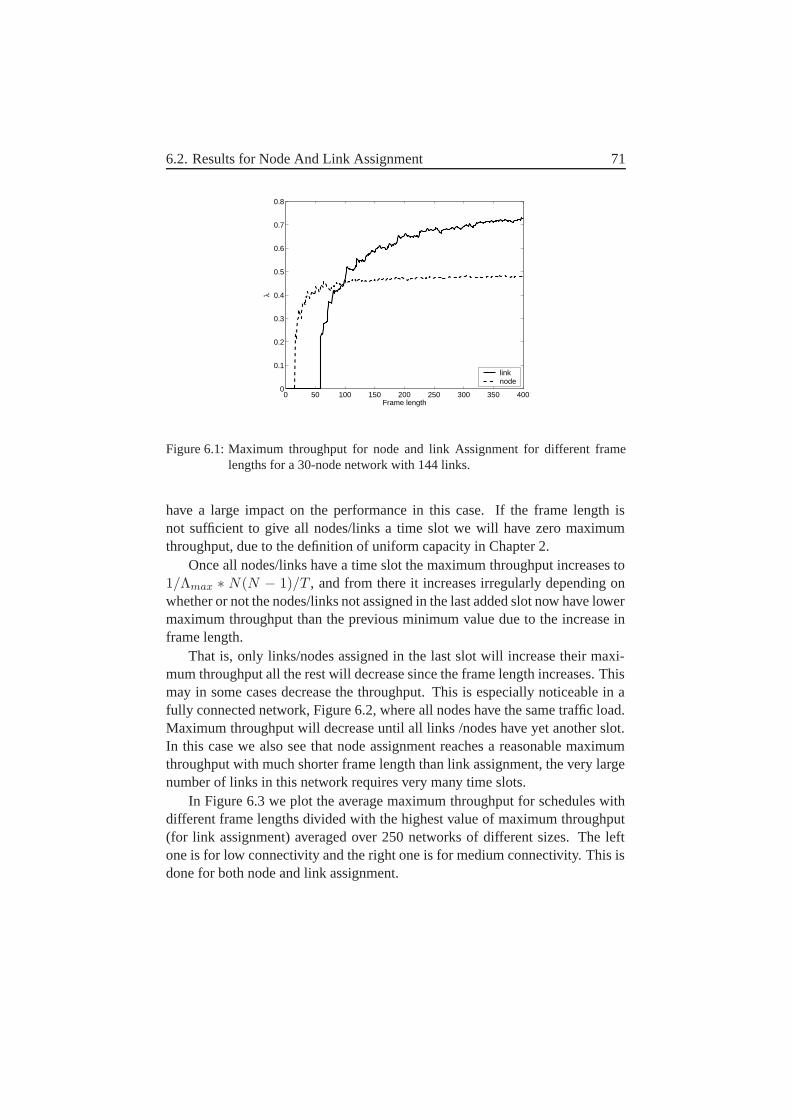
6.2. Results for Node And Link Assignment 71
0 50 100 150 200 250 300 350 4000
0.1
0.2
0.3
0.4
0.5
0.6
0.7
0.8
Frame length
λ
linknode
Figure 6.1: Maximum throughput for node and link Assignment for different framelengths for a 30-node network with 144 links.
have a large impact on the performance in this case. If the frame length isnot sufficient to give all nodes/links a time slot we will have zero maximumthroughput, due to the definition of uniform capacity in Chapter 2.
Once all nodes/links have a time slot the maximum throughput increases to1/Λmax ∗ N(N − 1)/T , and from there it increases irregularly depending onwhether or not the nodes/links not assigned in the last added slot now have lowermaximum throughput than the previous minimum value due to the increase inframe length.
That is, only links/nodes assigned in the last slot will increase their maxi-mum throughput all the rest will decrease since the frame length increases. Thismay in some cases decrease the throughput. This is especially noticeable in afully connected network, Figure 6.2, where all nodes have the same traffic load.Maximum throughput will decrease until all links /nodes have yet another slot.In this case we also see that node assignment reaches a reasonable maximumthroughput with much shorter frame length than link assignment, the very largenumber of links in this network requires very many time slots.
In Figure 6.3 we plot the average maximum throughput for schedules withdifferent frame lengths divided with the highest value of maximum throughput(for link assignment) averaged over 250 networks of different sizes. The leftone is for low connectivity and the right one is for medium connectivity. This isdone for both node and link assignment.
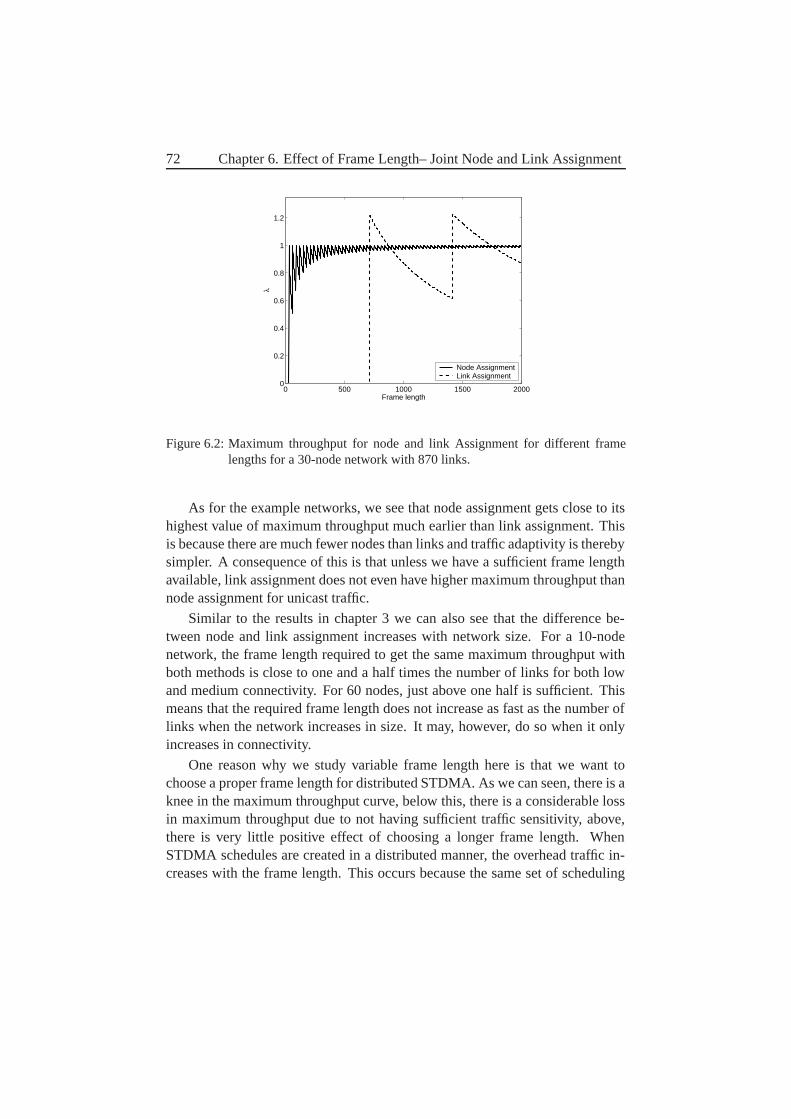
72 Chapter 6. Effect of Frame Length– Joint Node and Link Assignment
0 500 1000 1500 20000
0.2
0.4
0.6
0.8
1
1.2
Frame length
λ
Node AssignmentLink Assignment
Figure 6.2: Maximum throughput for node and link Assignment for different framelengths for a 30-node network with 870 links.
As for the example networks, we see that node assignment gets close to itshighest value of maximum throughput much earlier than link assignment. Thisis because there are much fewer nodes than links and traffic adaptivity is therebysimpler. A consequence of this is that unless we have a sufficient frame lengthavailable, link assignment does not even have higher maximum throughput thannode assignment for unicast traffic.
Similar to the results in chapter 3 we can also see that the difference be-tween node and link assignment increases with network size. For a 10-nodenetwork, the frame length required to get the same maximum throughput withboth methods is close to one and a half times the number of links for both lowand medium connectivity. For 60 nodes, just above one half is sufficient. Thismeans that the required frame length does not increase as fast as the number oflinks when the network increases in size. It may, however, do so when it onlyincreases in connectivity.
One reason why we study variable frame length here is that we want tochoose a proper frame length for distributed STDMA. As we can seen, there is aknee in the maximum throughput curve, below this, there is a considerable lossin maximum throughput due to not having sufficient traffic sensitivity, above,there is very little positive effect of choosing a longer frame length. WhenSTDMA schedules are created in a distributed manner, the overhead traffic in-creases with the frame length. This occurs because the same set of scheduling
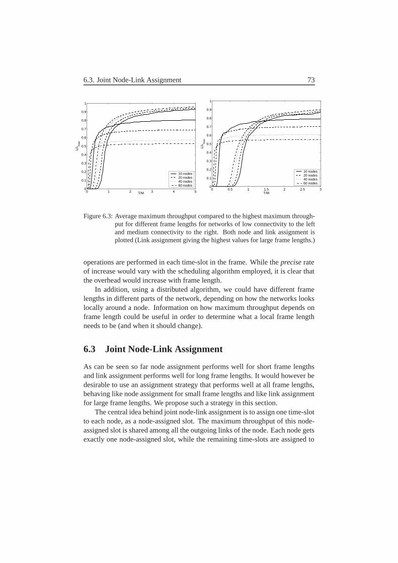
6.3. Joint Node-Link Assignment 73
0 1 2 3 4 50
0.1
0.2
0.3
0.4
0.5
0.6
0.7
0.8
0.9
1
T/M
λ/λ m
ax
10 nodes20 nodes40 nodes60 nodes
0 0.5 1 1.5 2 2.5 30
0.1
0.2
0.3
0.4
0.5
0.6
0.7
0.8
0.9
1
T/M
λ/λ m
ax
10 nodes20 nodes40 nodes60 nodes
Figure 6.3: Average maximum throughput compared to the highest maximum through-put for different frame lengths for networks of low connectivity to the leftand medium connectivity to the right. Both node and link assignment isplotted (Link assignment giving the highest values for large frame lengths.)
operations are performed in each time-slot in the frame. While the precise rateof increase would vary with the scheduling algorithm employed, it is clear thatthe overhead would increase with frame length.
In addition, using a distributed algorithm, we could have different framelengths in different parts of the network, depending on how the networks lookslocally around a node. Information on how maximum throughput depends onframe length could be useful in order to determine what a local frame lengthneeds to be (and when it should change).
6.3 Joint Node-Link Assignment
As can be seen so far node assignment performs well for short frame lengthsand link assignment performs well for long frame lengths. It would however bedesirable to use an assignment strategy that performs well at all frame lengths,behaving like node assignment for small frame lengths and like link assignmentfor large frame lengths. We propose such a strategy in this section.
The central idea behind joint node-link assignment is to assign one time-slotto each node, as a node-assigned slot. The maximum throughput of this node-assigned slot is shared among all the outgoing links of the node. Each node getsexactly one node-assigned slot, while the remaining time-slots are assigned to
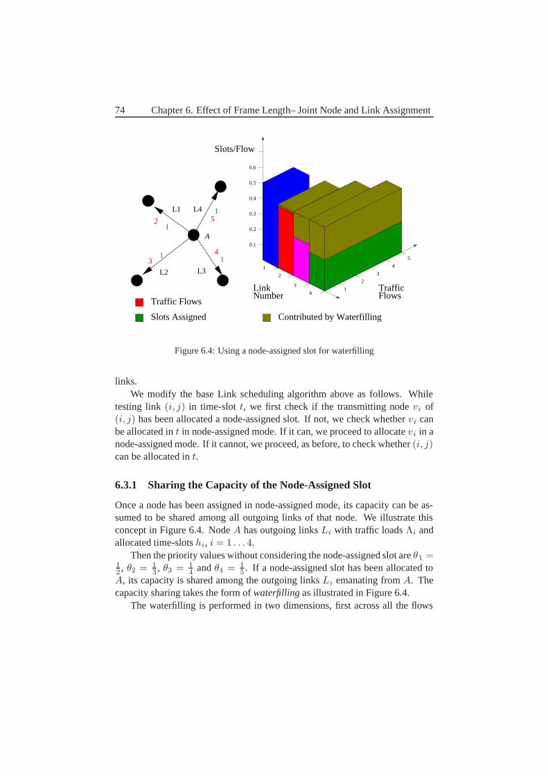
74 Chapter 6. Effect of Frame Length– Joint Node and Link Assignment
0.1
0.2
0.3
0.4
0.6
0.5
1
2
3
41
2
3
4
5
L2
2
31
1
15
41
L4
Link Traffic
Traffic Flows
Slots Assigned
Number Flows
Contributed by Waterfilling
Slots/Flow
L1
L3
A
Figure 6.4: Using a node-assigned slot for waterfilling
links.We modify the base Link scheduling algorithm above as follows. While
testing link (i, j) in time-slot t, we first check if the transmitting node vi of(i, j) has been allocated a node-assigned slot. If not, we check whether vi canbe allocated in t in node-assigned mode. If it can, we proceed to allocate vi in anode-assigned mode. If it cannot, we proceed, as before, to check whether (i, j)can be allocated in t.
6.3.1 Sharing the Capacity of the Node-Assigned Slot
Once a node has been assigned in node-assigned mode, its capacity can be as-sumed to be shared among all outgoing links of that node. We illustrate thisconcept in Figure 6.4. Node A has outgoing links Li with traffic loads Λi andallocated time-slots hi, i = 1 . . . 4.
Then the priority values without considering the node-assigned slot are θ1 =12 , θ2 = 1
3 , θ3 = 14 and θ4 = 1
5 . If a node-assigned slot has been allocated toA, its capacity is shared among the outgoing links Li emanating from A. Thecapacity sharing takes the form of waterfilling as illustrated in Figure 6.4.
The waterfilling is performed in two dimensions, first across all the flows
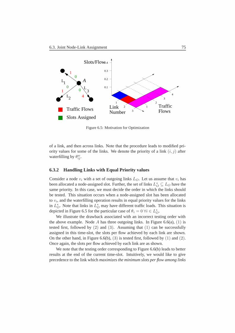
6.3. Joint Node-Link Assignment 75
0.1
0.2
0.3
0.4
1
2 1
2
3
4
Slots Assigned
Traffic Flows 3
01
4
0
TrafficLinkFlowsNumber
10
Slots/Flow
AL
L
1
2
3L
Figure 6.5: Motivation for Optimization
of a link, and then across links. Note that the procedure leads to modified pri-ority values for some of the links. We denote the priority of a link (i, j) afterwaterfilling by θw
ij .
6.3.2 Handling Links with Equal Priority values
Consider a node vi with a set of outgoing links LO. Let us assume that vi hasbeen allocated a node-assigned slot. Further, the set of links L∗
O ⊆ LO have thesame priority. In this case, we must decide the order in which the links shouldbe tested. This situation occurs when a node-assigned slot has been allocatedto vi, and the waterfilling operation results in equal priority values for the linksin L∗
O. Note that links in L∗O may have different traffic loads. This situation is
depicted in Figure 6.5 for the particular case of θi = 0 ∀i ∈ L∗O.
We illustrate the drawback associated with an incorrect testing order withthe above example. Node A has three outgoing links. In Figure 6.6(a), (1) istested first, followed by (2) and (3). Assuming that (1) can be successfullyassigned in this time-slot, the slots per flow achieved by each link are shown.On the other hand, in Figure 6.6(b), (3) is tested first, followed by (1) and (2).Once again, the slots per flow achieved by each link are as shown.
We note that the testing order corresponding to Figure 6.6(b) leads to betterresults at the end of the current time-slot. Intuitively, we would like to giveprecedence to the link which maximizes the minimum slots per flow among links
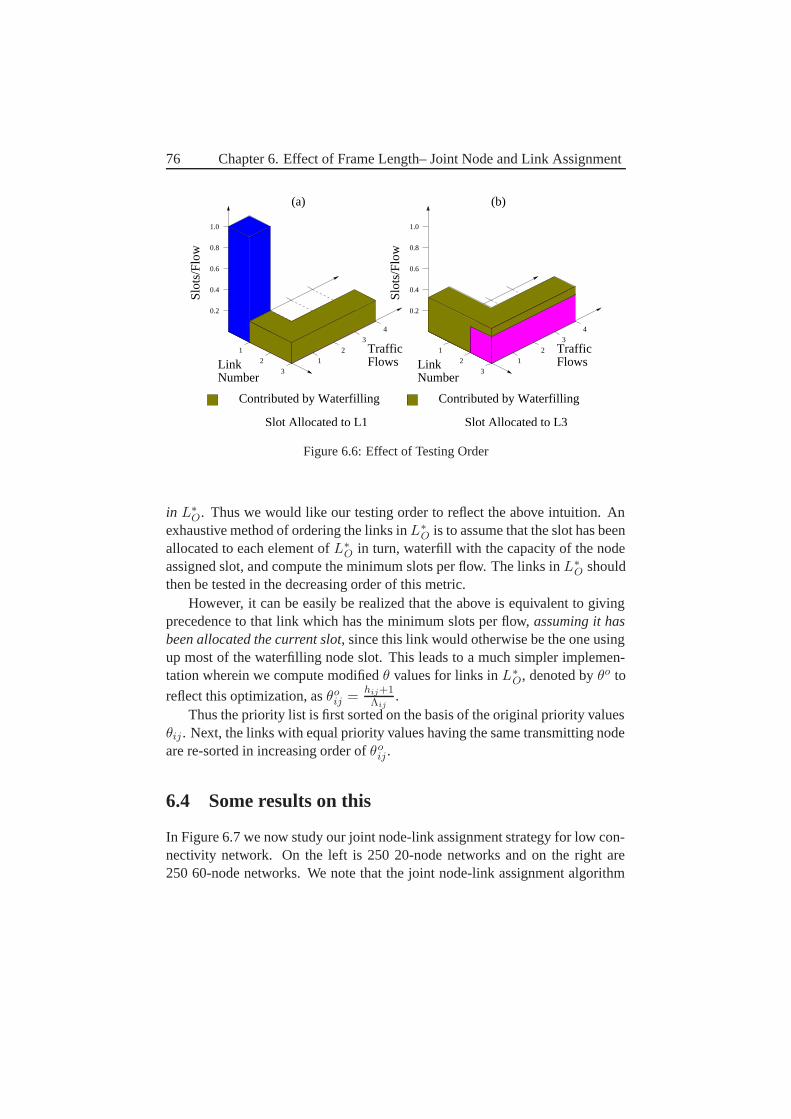
76 Chapter 6. Effect of Frame Length– Joint Node and Link Assignment
Contributed by WaterfillingContributed by Waterfilling
0.2
0.4
0.6
0.8
1
2
3
4
1.0
0.2
0.4
0.6
0.8
1
2
3
4
1.0
1
2
3
1
2
3Number
Traffic Flows
Traffic FlowsLink
Number
Slot Allocated to L1 Slot Allocated to L3
Slot
s/Fl
ow
Slot
s/Fl
ow
Link
(a) (b)
Figure 6.6: Effect of Testing Order
in L∗O. Thus we would like our testing order to reflect the above intuition. An
exhaustive method of ordering the links in L∗O is to assume that the slot has been
allocated to each element of L∗O in turn, waterfill with the capacity of the node
assigned slot, and compute the minimum slots per flow. The links in L∗O should
then be tested in the decreasing order of this metric.However, it can be easily be realized that the above is equivalent to giving
precedence to that link which has the minimum slots per flow, assuming it hasbeen allocated the current slot, since this link would otherwise be the one usingup most of the waterfilling node slot. This leads to a much simpler implemen-tation wherein we compute modified θ values for links in L∗
O, denoted by θo to
reflect this optimization, as θoij = hij+1
Λij.
Thus the priority list is first sorted on the basis of the original priority valuesθij . Next, the links with equal priority values having the same transmitting nodeare re-sorted in increasing order of θo
ij .
6.4 Some results on this
In Figure 6.7 we now study our joint node-link assignment strategy for low con-nectivity network. On the left is 250 20-node networks and on the right are250 60-node networks. We note that the joint node-link assignment algorithm
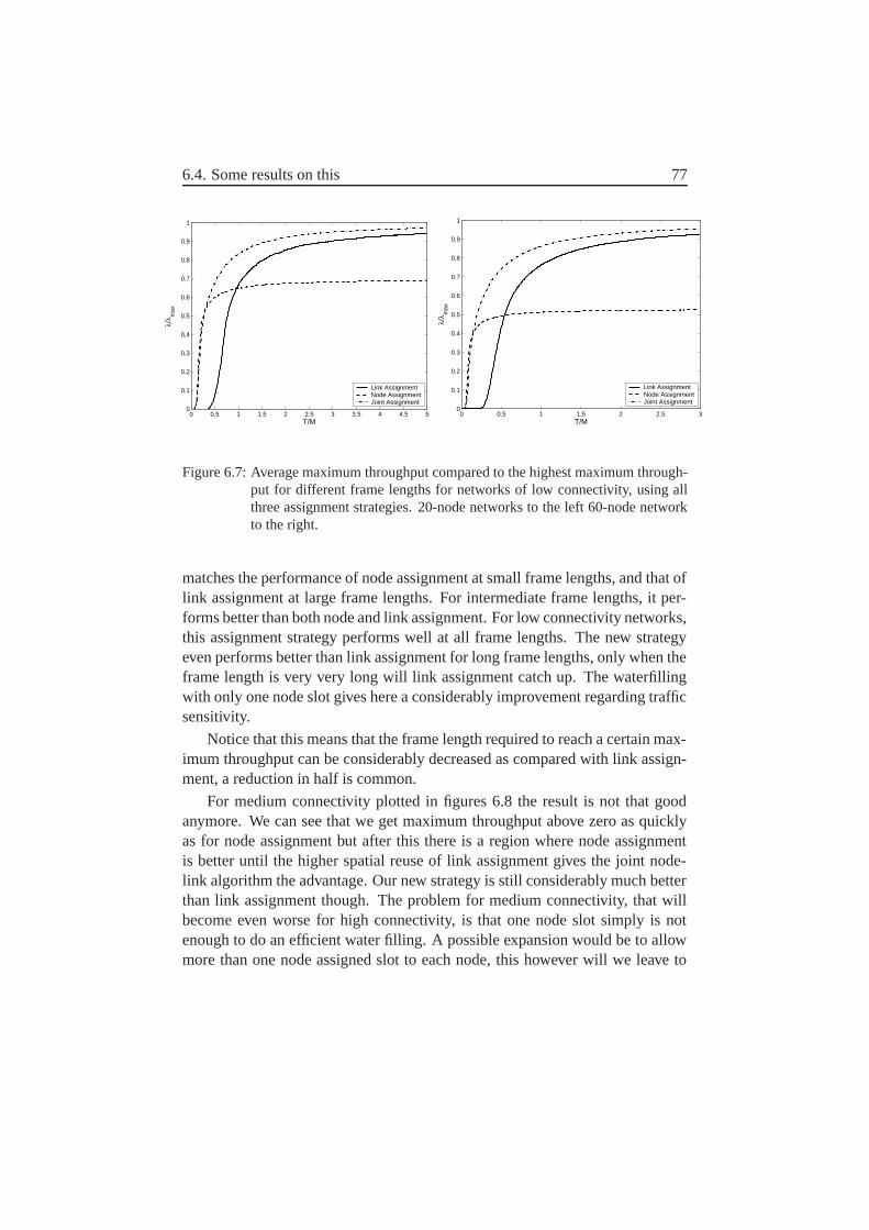
6.4. Some results on this 77
0 0.5 1 1.5 2 2.5 3 3.5 4 4.5 50
0.1
0.2
0.3
0.4
0.5
0.6
0.7
0.8
0.9
1
T/M
λ/λ m
ax
Link AssignmentNode AssignmentJoint Assignment
0 0.5 1 1.5 2 2.5 30
0.1
0.2
0.3
0.4
0.5
0.6
0.7
0.8
0.9
1
T/M
λ/λ m
ax
Link AssignmentNode AssignmentJoint Assignment
Figure 6.7: Average maximum throughput compared to the highest maximum through-put for different frame lengths for networks of low connectivity, using allthree assignment strategies. 20-node networks to the left 60-node networkto the right.
matches the performance of node assignment at small frame lengths, and that oflink assignment at large frame lengths. For intermediate frame lengths, it per-forms better than both node and link assignment. For low connectivity networks,this assignment strategy performs well at all frame lengths. The new strategyeven performs better than link assignment for long frame lengths, only when theframe length is very very long will link assignment catch up. The waterfillingwith only one node slot gives here a considerably improvement regarding trafficsensitivity.
Notice that this means that the frame length required to reach a certain max-imum throughput can be considerably decreased as compared with link assign-ment, a reduction in half is common.
For medium connectivity plotted in figures 6.8 the result is not that goodanymore. We can see that we get maximum throughput above zero as quicklyas for node assignment but after this there is a region where node assignmentis better until the higher spatial reuse of link assignment gives the joint node-link algorithm the advantage. Our new strategy is still considerably much betterthan link assignment though. The problem for medium connectivity, that willbecome even worse for high connectivity, is that one node slot simply is notenough to do an efficient water filling. A possible expansion would be to allowmore than one node assigned slot to each node, this however will we leave to
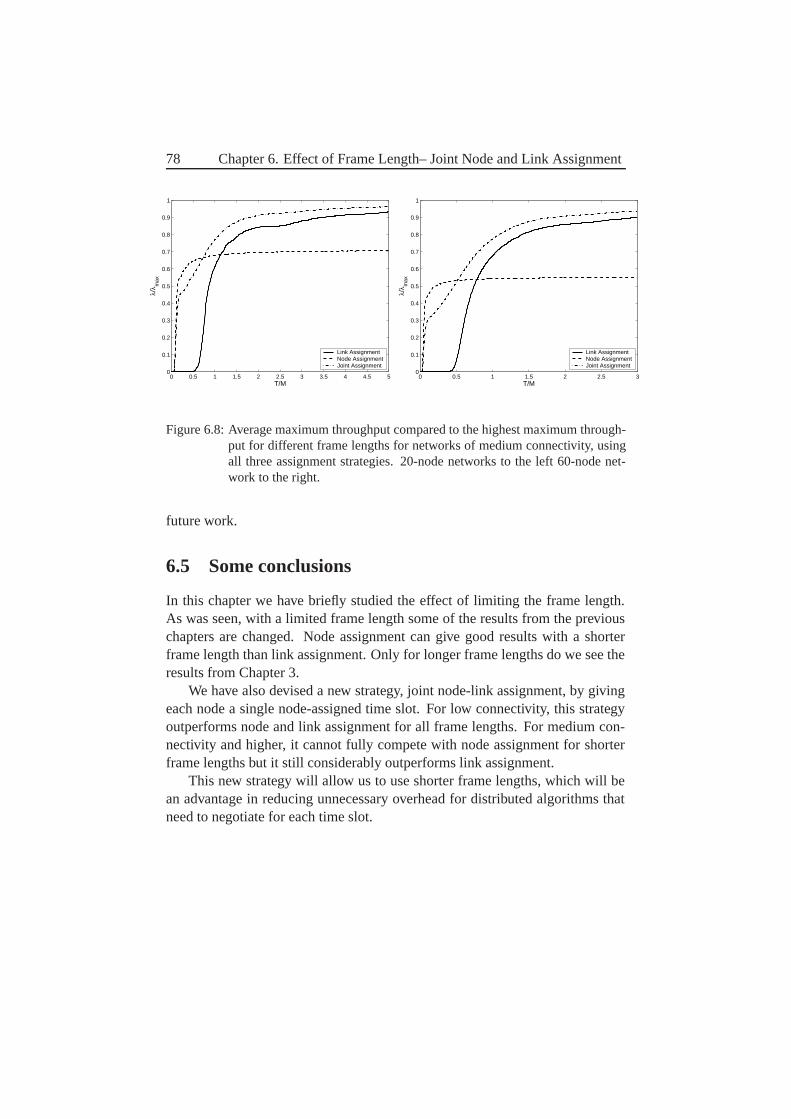
78 Chapter 6. Effect of Frame Length– Joint Node and Link Assignment
0 0.5 1 1.5 2 2.5 3 3.5 4 4.5 50
0.1
0.2
0.3
0.4
0.5
0.6
0.7
0.8
0.9
1
T/M
λ/λ m
ax
Link AssignmentNode AssignmentJoint Assignment
0 0.5 1 1.5 2 2.5 30
0.1
0.2
0.3
0.4
0.5
0.6
0.7
0.8
0.9
1
T/M
λ/λ m
ax
Link AssignmentNode AssignmentJoint Assignment
Figure 6.8: Average maximum throughput compared to the highest maximum through-put for different frame lengths for networks of medium connectivity, usingall three assignment strategies. 20-node networks to the left 60-node net-work to the right.
future work.
6.5 Some conclusions
In this chapter we have briefly studied the effect of limiting the frame length.As was seen, with a limited frame length some of the results from the previouschapters are changed. Node assignment can give good results with a shorterframe length than link assignment. Only for longer frame lengths do we see theresults from Chapter 3.
We have also devised a new strategy, joint node-link assignment, by givingeach node a single node-assigned time slot. For low connectivity, this strategyoutperforms node and link assignment for all frame lengths. For medium con-nectivity and higher, it cannot fully compete with node assignment for shorterframe lengths but it still considerably outperforms link assignment.
This new strategy will allow us to use shorter frame lengths, which will bean advantage in reducing unnecessary overhead for distributed algorithms thatneed to negotiate for each time slot.
Chapter 7
Distributed Information – Howto schedule Efficient?
All work so far have assumed a centralized scheduler, in practice this is un-wanted, by the time new information have been collected into a central unit itmay be obsolete, especially for a large network.
In addition, a centralized solution is not especially robust against node fail-ures. If the central unit is lost we may end up in serious problem, even if we havea backup node that can take over the scheduling. Therefore, we will now studydistributed scheduling, and see whether results from centralized scheduling canbe used also when we design distributed algorithms.
We will start this chapter by giving a list of the properties we seek in adistributed algorithm. We will also discuss whether existing algorithms for dis-tributed STDMA scheduling can handle these properties.
7.1 Wanted Properties
Although, many distributed STDMA algorithms are either node or link as-signed, commonly referred to node and link activation, many algorithm descrip-tions handle both of them. There is really little difference when we design adistributed algorithm — if we can design a distributed algorithm for one of themethods, it is not so much work to do the same for the other.
For distributed scheduling we will only concentrate on link assignment.In the following we list some of the desired properties of a distributed
STDMA algorithm. The first five of these are specific for distributed schedul-
79
80 Chapter 7. Distributed Information – How to schedule Efficient?
ing. The last three properties are general for all STDMA scheduling but theyare so relevant for performance so we repeat them here.
1. No central control; the algorithm is run in parallel in every node in thenetwork. This is necessary if we want a robust system that can handle theloss of any node and is the basic meaning of the term “distributed”.
2. Only local information is exchanged and needed. As the other corner-stone of the term “distributed”, the information propagation must be lim-ited. However, we do not make any specific definition of the term “local”,except that global information about the network is not needed.
3. Local adaptation to topological and traffic changes must be possible.(Ripples are permitted if the probability of updates decreases with dis-tance from the change.) This is an addition to the previous two assump-tions that prevent “unstable” algorithms.
4. The algorithm should be able to efficiently handle large changes in thenumber of nodes and density of the network. (By “efficiently” we meanthat it should not just be able to create a valid schedule but also performclose to the results of a centralized algorithm in a number of very differentscenarios). In particular, changes in the network density will be usual inmilitary scenarios and situations where all nodes are gathered at one place(with maximum density as a result) will occur.
5. The algorithm should adapt to the level of mobility. In relatively staticnetworks, we can get a very good picture of the situation, e.g. precisepath losses and power levels which could be used to make a more efficientschedule. In a high mobility network the only information that may bepossible to transmit might be the existence of neighbors. The algorithmshould perform well under these circumstances too. The radio channelis the scarce resource in our network and should be used as efficiently aspossible.
6. Adaptivity to traffic; the algorithm should be able to adapt to the differentneeds of the different links. There is considerable variation of traffic overthe different links of the network due to the relaying of traffic in multi-hopnetworks. An STDMA algorithm must adapt to this in order to be efficient[30]. Furthermore, one of the main advantages of STDMA is its ability
7.1. Wanted Properties 81
to provide QoS. In order to go beyond one slot per frame guarantees (oreven reach this for a single flow), traffic adaptivity is a must.
7. Using an interference-based network model. The graph-based networkmodel is currently the most used network model for ad hoc-networks.However, this model does not reflect reality sufficiently well in many ofour scenarios. As was shown in chapter 5, graph-based scheduling do notperform very well compared to interference-based scheduling.
8. The algorithm should handle (exploit) heterogeneous nodes in the net-work. Some nodes may have more advanced abilities than others, e.g.adaptive antennas, able to use variable data rate, lower noise levels andsimilar abilities. Moreover, a node might have the same radio as the restof the nodes but have other properties, e.g. in terms of mobility. A heli-copter is one example of this kind of node, another is a node that is knownto be immobile.
The first three of these properties are handled by all algorithms that claim tobe distributed, although point three is difficult to assess without actual simula-tions. For the rest of the properties there are considerable variations.
Many algorithms need at least information about the number of nodes andnode density. Actually, several papers, see e.g. [17, 32], prove that their algo-rithm can create schedules with length dependent on the maximum density ofthe network. However, unless methods not mentioned in the papers are added,this gives a fixed frame length throughout the network. This means that a changein the number of nodes or an increase in network density might force a globalupdate of the network. This will probably not happen as often as normal up-dates, but it is still highly undesired. To avoid such global updates these pa-rameters must be chosen to be worst case, which usually results in unnecessarycomplexity and inefficiency. Therefore, fixing the length of the schedule is asimple solution, but it does not handle the situation of varying the number ofnodes in the network very well. If the number of nodes increases and the net-work density gets high (many neighboring nodes), the fixed frame length maynot be sufficient. If the number of nodes decreases, this may result in an unnec-essary long schedule with its added load of complexity. In many algorithms, seefor example [15, 17, 32], we end up with a schedule of fixed length (or less thanthis length) depending on the network density and size.
However, there are a better approach, that we could call the 2n principle,used in [36, 20, 16]. The frame length is varied in different parts of the network
82 Chapter 7. Distributed Information – How to schedule Efficient?
(and also over time). The frame length as seen by a node or a link is of length2n. If the density increases in a local area, n can be increased by one in thisarea. This does not cause any changes outside this local area. If all nodes inthe area can receive their slots in the first half of the frame, the schedule can bedecreased.
It is difficult to say how well this works and how efficient schedules arecreated if we have large changes in the number of nodes and/or density, but it isa method worth investigating further.
As mentioned in chapter 1, traffic control is only rarely included in the dis-tributed algorithms. Although some algorithms include the ability to assignmore than one time slot to a link or node, see e.g. [36, 37], a more specific de-scription of how and when some of the links receive extra time slots is usuallyomitted.
Most distributed STDMA algorithms assume a very simple graph model,which can give poor results, see chapter 5, and usually they are not easily ex-panded to an interference-based model. Many can be expanded to a two-levelgraph model, but this gives a considerable decrease in maximum throughputcompared with an interference-based model. One exception to the use of graph-based scheduling is [68], but this paper investigates extremely large systems anddoes not use time slotted systems.
The existing distributed algorithms are generally designed for the high mo-bility case, and the graph model does not convey sufficient network informationfor efficient scheduling in a more stable scenario. For high mobility, though, it isprobably not possible to convey more than this information, which suggests thatthe accuracy of network information should decrease with increasing networkmobility. How much information should be conveyed to the local neighborhoodfor a specific mobility rate (as compared to the link data rate) is still an openissue. For very high mobility we might end up with the same information as agraph model gives.
A lot of work has been done on distributed STDMA, but no existing al-gorithm fulfills all our required properties. Of the existing algorithms, USAPis probably the most interesting for military communications but not even thisalgorithm has all the listed properties that are desired for reliable and efficientcommunication on the battlefield.
However, although none of these algorithms can fulfill our properties theyhave functions that will be useful when designing such an algorithm.
All distributed algorithms have been designed with the purpose of giving anacceptable solution, rather than a solution that handles the channel as efficiently
7.2. An Interference-Based Distributed Algorithm 83
as possible under different situations. A more systematic approach to the designof distributed STDMA algorithms is lacking. What is an efficient schedule in aspecific scenario? How is such a schedule created? Exactly which informationis needed and how much in each case?
We know that the more information about the network we have the bet-ter schedules we can create, thereby increasing the total maximum throughputof the network. However, increasing information also increases the overhead.This means that the amount of information the algorithm has about the networkshould vary depending on the situation.
The use of interference-based scheduling can give us the means to vary theamount of information. So far no distributed STDMA algorithms have tried touse this.
In the rest of the chapter we will describe our proposal to an interference-based STDMA algorithm that creates an efficient schedule with a given amountof information about the network.
In this chapter our algorithm does not care how it receives the information,but simply acts on the information it has received. The purpose of this is to in-vestigate how efficiently we can use distributed information. In the next chapterwe will study how to convey the required information.
7.2 An Interference-Based Distributed Algorithm
In short, the our distributed STDMA algorithm can be described by the follow-ing steps:
• Nodes that have entered the network exchange local information withtheir neighbors.
• The link with highest priority in its local surroundings assigns itself a timeslot (this is done in the receiver).
• The local schedule is then updated, and a new link has highest priority.This process is then continued until all slots are occupied.
We will include traffic sensitivity through the link priorities, i.e. a link thatneeds many time slots will have high priority more often than a link with lowpriority.
The algorithm is interference-based since it uses interference information,i.e. interference information is transmitted and used when the algorithm decide
84 Chapter 7. Distributed Information – How to schedule Efficient?
when links can transmit simultaneously. We will use the term local neighbor-hood of a link (i, j) to mean those links that will be taken into considerationwhen a link determines whether it can transmit simultaneously with all otherassigned links. Links outside the local neighborhood will not be considered andtherefore no information about these links is assumed. Exactly how large thisneighborhood is will be discussed later.
In the following we will assume that each link has a given schedule lengthT . This length is not necessarily the same length in all parts of the network andmay change over time. But this will not change the basic scheduling process.
7.2.1 Link States
The STDMA algorithm is run in parallel for each link, i.e. each link can be seenas a separate process which will be run at the receiving node of the link, whichmeans that each node will run a process per incoming link. These processes canbe in three states: active, waiting, or asleep.
• Active: In this mode, the link has the highest priority in its local neigh-borhood and will subsequently assign itself a time slot. Which time slotis chosen if more than one is available will be discussed later. A linkprocess can be in this mode because of the existence of unused slots orbecause the link’s share of the time slots in its local neighborhood is toolow. In the latter case, it can steal time slots from another link. We willdescribe later under which situations this may be permitted. Informationabout which time slot is chosen and the link’s new priority will be trans-mitted to all nodes in the local neighborhood of the link. After this, thelink process can stay in this mode or change into one of the others.
• Waiting: In this mode the links wants to assign itself a time slot, butanother link has highest priority. The link will wait its turn. However,since time slots are taken by active users, the link may change into asleepmode instead if all time slots are taken and the link does not have the rightto steal slots.
• Asleep: In this mode, there are no available slots for the link and it simplywaits for a change of the network, either in topology or in traffic levels.
The purpose of the sleeping phase is that to let also nodes that are not high-est prioritized allocate time slot. This will allow us to use the channel moreefficiently. In the next chapter we look into this in more detail.
7.2. An Interference-Based Distributed Algorithm 85
7.2.2 Link Priority
Link priority decides in which order the links may attempt to assign themselvesa time slot. The link priority can depend on many things, but the most importantwill be the number of time slots the link is assigned, hij , and the traffic of thelink, Λij . Since both these values are changing, the link priority is constantlychanging.
The priority value of a link (i, j) will be hij
Λij, where the lowest value has the
highest priority. The motivation for this comes from the maximum throughputformula (3.5). The links with the highest priority (lowest value) will be the linkswhich limit the maximum throughput of the network. The network throughputwill not rise above zero until all links with traffic levels above zero have receivedat least one time slot. An obvious consequence of this is that all links with trafficin a local neighborhood will receive at least one time slot before any of the linksreceive more than one slot. This will be the case, for example, when a newschedule is initiated.
7.2.3 Theft of Time slots
Sometimes, the relative traffic levels will change in a local area (or other changesmay take place). This will result in a situation where a link has a smaller pro-portion of the time slots than its priority value merits. If there are free slots, thelink may assign itself slots until it is on a similar priority level as its surroundinglinks. However, if no time slots are free, the link can sometimes steal time slotsfrom other nodes.
The policy for assigning time slots in the case of free time slots is alwaysthat the link which limits the maximum throughput will be the one that receivesan extra time slot. This is also the case when a link is permitted to steal a timeslot. When stealing a time slot, the local network throughput must increase.
This means that a link (i, j) is only permitted to steal a time slot from an-other link (k, l) if the priority value of the stealing link is lower than the otherlink’s priority value after the loss of a time slot, i.e.
hij
Λij<
hkl − 1Λkl
.
The theft of time slots means that it is the link with too few time slots thatreacts to unfairness situations. This is a better solution than if links that havetoo many time slots would give them up since such a link can never know if
86 Chapter 7. Distributed Information – How to schedule Efficient?
the time slot can be used by the link with too few time slots. The time slot canalways be blocked by another node further away.
In this form, the algorithm permits the theft of a time slot if there is anygain at all independent on how small. Since this always will result in additionaloverhead traffic we may want to limit the cases where theft is allowed to onlycases where the maximum-throughput gain is worth the overhead cost.
One way of doing this is to include a Theft Threshold (TT) such that theftis allowed iff:
hij
ΛijTT <
hkl − 1Λkl
,
where TT is greater than or equal to one. As we will see in the next chapter, thesetting of this parameter can affect the maximum throughput and overhead. Tostart with we will use TT equal to one.
7.2.4 Choice of time slots
Sometimes when a node attempts to assign itself a time slot, it will have morethan one to choose from. This will especially be the case when the scheduleis first initiated. The main reason why the choice of time slot is important isthe packet delay of the network. For example, if a link has received two timeslots and these are spread in such a way that the distance between them is ap-proximately half the frame length, then for low traffic loads the delay will be atmost half the frame length. However, if the node is given two consecutive timeslots, the maximum delay might be the entire frame length. That is, it is usuallyefficient to spread a node’s time slots evenly over the frame. This problem getsworse if nodes receive many time slots, especially since a large part of the trafficusually flows through these nodes. From this small example we can concludethat the choice of time slots can be important.
Note that this can also affect the links that will receive only a single timeslot. The reason for this is that all links will receive one slot before any ofthem receive their second. If we use up all slots in the first half of the schedule,for instance, we will not have an efficient spreading of time slots. This can bealleviated by choosing a time slot at random when we choose the first time slotfor a link. When the link already has time slots assigned to it, we choose a slotthat is maximally spread from the others.
Another reason for this consideration can be the existence of weak links,i.e. links that can only handle very small amounts of interference. These linksare difficult to assign to the same slot as any other link unless they are very
7.2. An Interference-Based Distributed Algorithm 87
far apart. Another property of these links is that they are often long, i.e. theycarry traffic a long physical distance in one hop. The links will often be used byrouting algorithms that do not take into consideration the capacity of the link,a property that describes virtually all existing ad hoc routing algorithms, thusresulting in heavy traffic loads. Due to the high traffic loads these links usuallyreceive several time slots. Now, if all the stronger links have received a timeslot each, unused by any other node, it might be difficult to give the weak linkstheir extra slots. Therefore, it can be a good idea to try to assign strong links,those that can handle larger interference levels, to slots where the interferencelevels already are rather high (not too high of course) and leave the unused(low interference level) slots to weak links. However, this might be a complexprocedure, so we will leave such an investigation for the future.
In addition to this we have the same problem when when a link wants tosteal a time slot, if there are more than one available it can be an advantage tosteal the time slot, where the resulting maximum throughput is highest. That is,we may only steal time slots is there is a gain in maximum throughput by doingit, but how large that gain is can be dependent on which time slot that is stolen.The links that lose a time slot may now be the limiting links instead of thestealing link for example. The choice of time slot can thereby be of importance.
For simplicity, and the fact that we only evaluate maximum throughput inthis report, we have chosen the first available time slot when doing normal as-signment in our simulations. For theft we have chosen the time slot whoseassigned links (only those that we actually steal) have the highest priority valueafter they loose a time slot.
7.2.5 When do we have a re-scheduling?
We have so far described the different states of a link process and how the pri-ority is calculated, but we have not been very detailed about the circumstancesunder when a new scheduling event take place. In the following, we give eventsthat can cause changes in an ad hoc network and which consequences they have.
• Increased interference level on a link due to mobility. The link cannot usethe slot and deallocates it. This has two consequences. First, hij decreasesfor the link which decreases the priority value for the link. The link maynow have a value so low that it is permitted to steal a time slot fromanother node. Second, since the link deallocates the time slot, anotherlink may now have a free slot, which it may allocate itself.
88 Chapter 7. Distributed Information – How to schedule Efficient?
• Decreased interference level on a link due to mobility. A link may have afree time slot that was previously blocked, which it will allocate to itself.This increases hij , which might result in another link stealing a time slotfrom the link.
• A link breaks: This stops the link process, and all assigned time slots willbe deallocated. This will have similar consequences as when a link givesup a time slot due to interference, although this can happen to many timeslots simultaneously, thus affecting more links. However, a link break canalso have consequences for the routing, which affects Λij . The priorityvalues in the neighborhood, or even further away, may change. This maylead to significant schedule changes.
• A link is created: This creates a new link process (or restarts an earlierprocess). We make the assumption that Λij for the new link is set to avalue greater than zero, which results in a priority value of zero. Thismeans that the link will assign itself a time slot if one is available orotherwise steal one from a link with more than one time slot. A new linkcan also lead to a rerouting of the traffic, which may have consequencesfurther away.
• A new node is added to the network: This can be seen as several links thatare added simultaneously. It can also change traffic in the network.
• A node disappears from the network: This can be seen as the removal ofseveral links at once. It can also change traffic in the network.
• Rerouting or other traffic changes: This can result from link failures, linkscreated or changes in the input traffic to the network. This changes thepriority of the links, which can cause time slots to be stolen.
Some other things can also be mentioned. First, with more complex linkswe may have a variable link data rate. In such a case hij may not necessarilybe an integer. Second, if a link has one of its time slots stolen, it sometimeshas the opportunity to steal a time slot from a link further away from the linkthat initiated the theft. Third, it is also possible that the local frame length isnot sufficiently long for as much traffic adaptivity as we would like, or evenlong enough to give all links a single time slot. In this case, the local framelength must be increased. However, we will leave how this is done and how wedetermine whether it is necessary for future work.
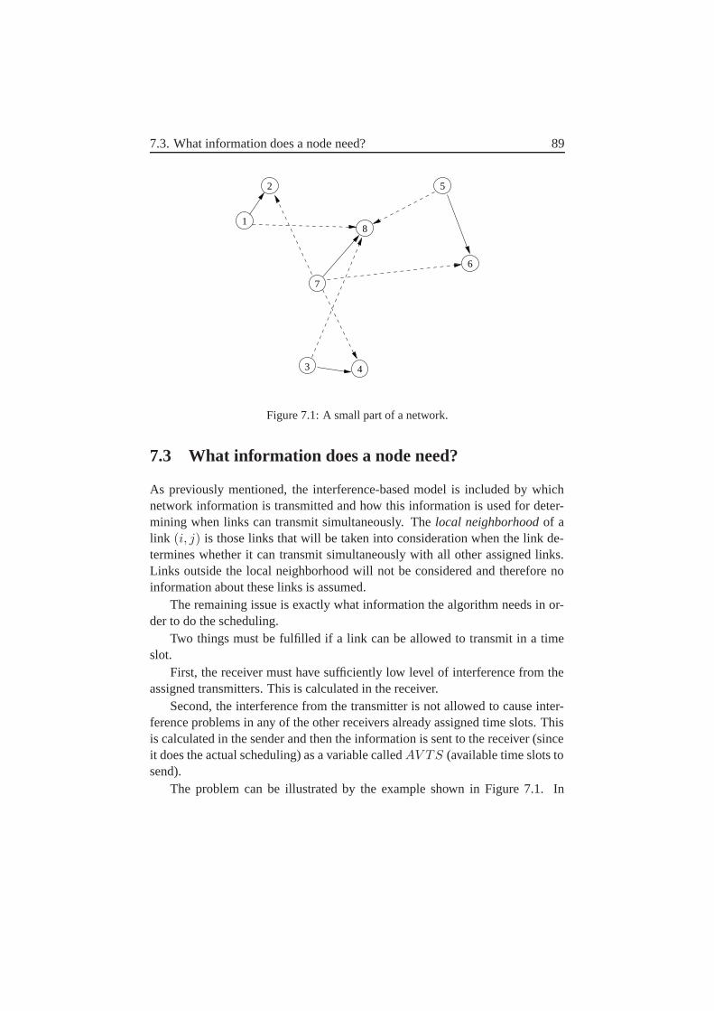
7.3. What information does a node need? 89
1
2
3 4
5
6
8
7
Figure 7.1: A small part of a network.
7.3 What information does a node need?
As previously mentioned, the interference-based model is included by whichnetwork information is transmitted and how this information is used for deter-mining when links can transmit simultaneously. The local neighborhood of alink (i, j) is those links that will be taken into consideration when the link de-termines whether it can transmit simultaneously with all other assigned links.Links outside the local neighborhood will not be considered and therefore noinformation about these links is assumed.
The remaining issue is exactly what information the algorithm needs in or-der to do the scheduling.
Two things must be fulfilled if a link can be allowed to transmit in a timeslot.
First, the receiver must have sufficiently low level of interference from theassigned transmitters. This is calculated in the receiver.
Second, the interference from the transmitter is not allowed to cause inter-ference problems in any of the other receivers already assigned time slots. Thisis calculated in the sender and then the information is sent to the receiver (sinceit does the actual scheduling) as a variable called AV TS (available time slots tosend).
The problem can be illustrated by the example shown in Figure 7.1. In
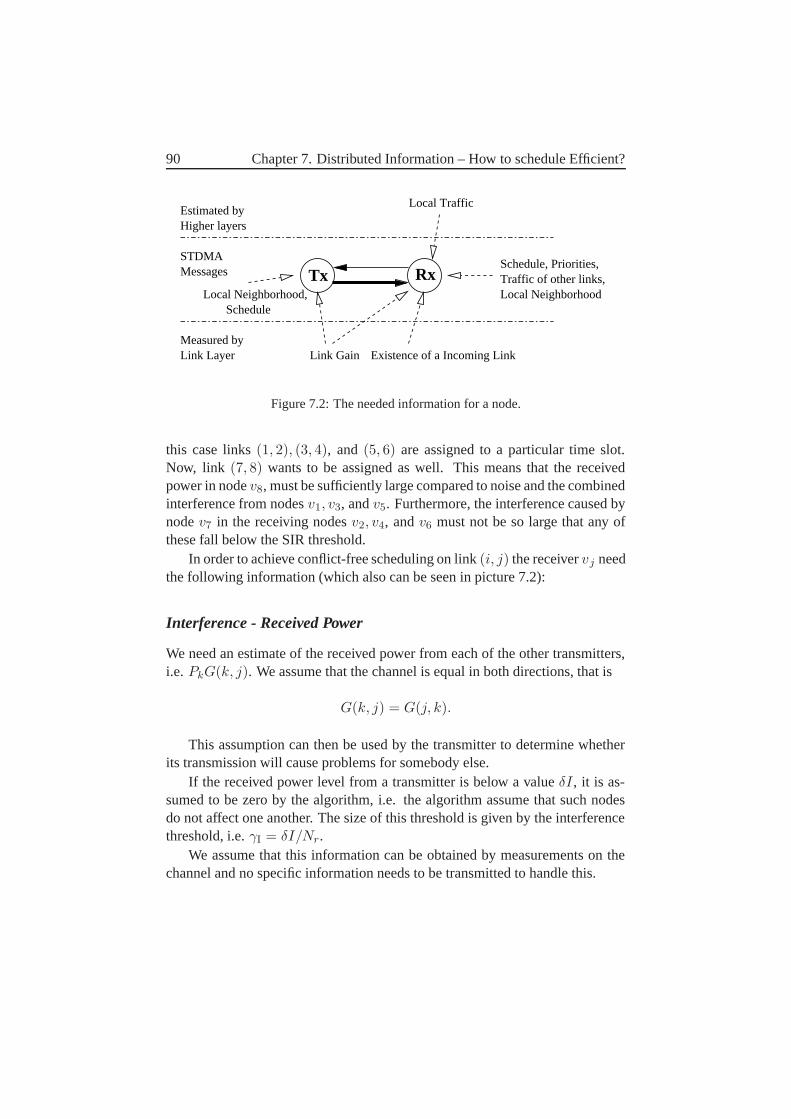
90 Chapter 7. Distributed Information – How to schedule Efficient?
RxTx
Measured by
Estimated byHigher layers
Link Layer
Local Neighborhood
Messages
Schedule
STDMA
Local Neighborhood,
Local Traffic
Link Gain Existence of a Incoming Link
Traffic of other links,Schedule, Priorities,
Figure 7.2: The needed information for a node.
this case links (1, 2), (3, 4), and (5, 6) are assigned to a particular time slot.Now, link (7, 8) wants to be assigned as well. This means that the receivedpower in node v8, must be sufficiently large compared to noise and the combinedinterference from nodes v1, v3, and v5. Furthermore, the interference caused bynode v7 in the receiving nodes v2, v4, and v6 must not be so large that any ofthese fall below the SIR threshold.
In order to achieve conflict-free scheduling on link (i, j) the receiver vj needthe following information (which also can be seen in picture 7.2):
Interference - Received Power
We need an estimate of the received power from each of the other transmitters,i.e. PkG(k, j). We assume that the channel is equal in both directions, that is
G(k, j) = G(j, k).
This assumption can then be used by the transmitter to determine whetherits transmission will cause problems for somebody else.
If the received power level from a transmitter is below a value δI , it is as-sumed to be zero by the algorithm, i.e. the algorithm assume that such nodesdo not affect one another. The size of this threshold is given by the interferencethreshold, i.e. γI = δI/Nr.
We assume that this information can be obtained by measurements on thechannel and no specific information needs to be transmitted to handle this.
7.3. What information does a node need? 91
To simplify notation, we say that a pair of nodes vi and vj form a interfer-ence link if the signal-to-noise ratio (SNR) is less than γC but higher than γI ina similar way as in chapter 5.
Local Schedule
A node needs to know the local schedule and how much more interference canbe handled by the assigned receivers Imax(l, τ) in each time slot τ , i.e. thelargest value of Imax such that the following inequality is still valid
PkG(k, l)(Nr + IL(k, l) + Imax(l, τ))
≥ γR.
This information (Imax(l, τ)) is required for node vi to be able to determinewhether its transmission can be handled by the other, already assigned receivers.A link can be assigned the time slot if:
PiG(i, l) < Imax(l, τ)
for all assigned receivers vl in time slot τ .The local schedule is also used to determine whether the receiver vj can
handle all existing interference. Measurements of the channel in the specifictime slot can be of help when doing this, but is not sufficient since node vj
cannot know whether all assigned transmitters vk actually are using their timeslot. Instead the actual SIR is calculated using the local schedule and receivedpower levels. If the interference levels that are measured are higher than thisestimate, we conclude that the we have extra interference from outside the localneighborhood and the interference measured should be used while this lasts.
The local schedule S and all values of Imax(l, τ) needs to be sent over thechannel. However, only information about nodes that vj can cause interferenceto or vj can be interfered by is needed.
Priorities
A node needs to know when it should be active. It also needs to know if a nodein the neighborhood is asleep, since such nodes are not considered in terms ofpriority. The exception to this is the case with theft of time slots, in whichcase sleeping nodes are also considered. The node needs such information fromthe entire local neighborhood since we cannot allow two nodes to be activesimultaneously in the local neighborhood.
92 Chapter 7. Distributed Information – How to schedule Efficient?
Available Time Slots to Send (AVTS)
The receiver also needs information from the transmitter about which time slotsit can assign. This can be represented by a vector of the same length as theframe length or specific information about changes of a single time slot. Onlyinformation from the transmitter is needed by the receiver.
With this information the receiver has sufficient information to determinewhen link (i, j) should be active and which time slots it can assign.
Local neighborhood
Due to mobility the local neighborhood will change constantly and we also needto have accurate information about what the local neighborhood is at the presentmoment.
7.3.1 Continues Variables
A problem with interference-based scheduling that does not exist for graph-based scheduling is that some of the parameters used are not discrete variables,an example of such a parameter is path-loss. Such variables may take any valueand can change continuously. Path-loss need not to be sent but Imax is dependenton path-loss values and need to be sent.
In practice, also path-loss values and measured values of interference willbe sampled, by lower layers, but this may be of too high rate change each suchvalue to be sent to the local neighborhood.
To avoid this we can introduce another threshold Imax Threshold (IMT), thatwill be the minimum change of Imax that will cause an update.
7.3.2 Consequences of limited information
A problem with limiting the input information on the network, i.e. using theinterference threshold, is that units from far away are not considered. Althoughthese nodes create small interference in a node, they might still cause a prob-lem since the nodes will try to schedule as many links as possible in each timeslot. This means that the scheduled SIR will be very close to γR in many re-ceivers. The additional interference from outside the local neighborhood canthen be sufficient to lower the actual SIR below γR. One way to avoid this isto use an interference margin Imargin, i.e. we assume that there will be external
7.4. Instantaneous Maximum Throughput 93
interference and therefore avoid scheduling the SIR as low as γR. The link isthen assumed to be able to use the time slot if:
PiG(i, j)(Nr + IL(i, j) + Imargin)
≥ γR.
However, this solution may not completely solve the problem. One reasonis efficiency—in order to completely avoid the problem we have to choose arather large margin, which means that the channel will be used poorly. A secondreason is network connectivity; a high interference margin will prevent the useof weak links, which might cause the network to partition. Therefore, alternativesolutions may be required.
The method we will use in this thesis is to decrease the data rate for thoselinks that have received time slots with too low SIR. To do this we measure (orestimate) the actual SIR when the schedule is used and lower the data rate untilreliable communication is possible.
This is doable to a certain limit. If the external interference is very high,outside our control, we might finally give up the time slot entirely, set the timeslot as unavailable, and attempt to assign a new slot if this is allowed, and hopeto achieve a better SIR.
Another problem with lowering the data rate was shown is chapter 2, that istraffic sensitivity. Remember that the priority of a link is based on how loadedthe link is. This is dependent on how many time slots the link is assigned.If these slots do have a lower data rate than assumed when the time slot wasassigned, it means that the link in practice has lower maximum throughput thanit should. This effect will be seen in the simulations. However, this can be easilysolved by assuming that hij is not an integer and that it decreases when the datarate decreases. For example, if a link has three times slots allocated, two at fullrate and one at half rate, hij will be two and a half for this link.
In the following we assume that this is done. In the next chapter we willstudy the consequences of these methods.
7.4 Instantaneous Maximum Throughput
We will now study some cases where we run the algorithm. In Figure 7.3 weshow the instantaneous maximum throughput for a mobile network for both thedistributed algorithm as well as the centralized algorithm presented in chapter6. The network is a 32-node network where all nodes moves randomly with a
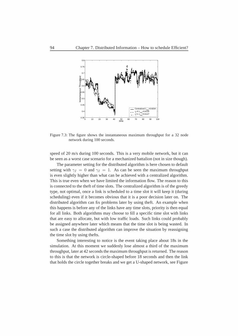
94 Chapter 7. Distributed Information – How to schedule Efficient?
0 10 20 30 40 50 60 70 80 90 1000.35
0.4
0.45
0.5
0.55
0.6
0.65
0.7
0.75
0.8
time
Inst
anta
neou
s T
hrou
ghpu
t
Centralized λavg
=0.6034γI=0 λ
avg=0.6132
γI=1 λ
avg=0.6127
Figure 7.3: The figure shows the instantaneous maximum throughput for a 32 nodenetwork during 100 seconds.
speed of 20 m/s during 100 seconds. This is a very mobile network, but it canbe seen as a worst case scenario for a mechanized battalion (not in size though).
The parameter setting for the distributed algorithm is here chosen to defaultsetting with γI = 0 and γI = 1. As can be seen the maximum throughputis even slightly higher than what can be achieved with a centralized algorithm.This is true even when we have limited the information flow. The reason to thisis connected to the theft of time slots. The centralized algorithm is of the greedytype, not optimal, once a link is scheduled to a time slot it will keep it (duringscheduling) even if it becomes obvious that it is a poor decision later on. Thedistributed algorithm can fix problems later by using theft. An example whenthis happens is before any of the links have any time slots, priority is then equalfor all links. Both algorithms may choose to fill a specific time slot with linksthat are easy to allocate, but with low traffic loads. Such links could probablybe assigned anywhere later which means that the time slot is being wasted. Insuch a case the distributed algorithm can improve the situation by reassigningthe time slot by using thefts.
Something interesting to notice is the event taking place about 18s in thesimulation. At this moment we suddenly lose almost a third of the maximumthroughput, later at 42 seconds the maximum throughput is returned. The reasonto this is that the network is circle-shaped before 18 seconds and then the linkthat holds the circle together breaks and we get a U-shaped network, see Figure
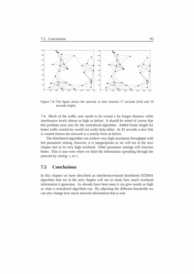
7.5. Conclusions 95
0 500 1000 1500 2000 2500 3000 3500 40000
500
1000
1500
2000
2500
3000
3500
4000
0 500 1000 1500 2000 2500 3000 3500 40000
500
1000
1500
2000
2500
3000
3500
4000
Figure 7.4: The figure shows the network at time instance 17 seconds (left) and 18seconds (right).
7.4. Much of the traffic now needs to be routed a far longer distance whileinterference levels almost as high as before. It should be noted of course thatthis problem exist also for the centralized algorithm. Added frame length forbetter traffic sensitivity would not really help either. At 42 seconds a new linkis created returns the network to a similar form as before.
The distributed algorithm can achieve very high maximum throughput withthis parameter setting, however, it is inappropriate as we will see in the nextchapter due to its very high overhead. Other parameter settings will functionbetter. This is true even when we limit the information spreading through thenetwork by setting γI to 1.
7.5 Conclusions
In this chapter we have described an interference-based distributed STDMAalgorithm that we in the next chapter will use to study how much overheadinformation it generates. As already have been seen it can give results as highas what a centralized algorithm can. By adjusting the different thresholds wecan also change how much network information that is sent.
96 Chapter 7. Distributed Information – How to schedule Efficient?
Chapter 8
Distributed Information–Atwhat cost?
In this chapter we will study what information the nodes need to convey to theother nodes in their local neighborhood, how often such messages need to besent, and, finally, determine the overhead for some different networks.
8.1 What Information Must Each Node Send and to WhichReceivers?
At the end of the previous chapter we showed what information a node needsto make a correct decision about whether it can assign a time slot or not. Inthis section we will look at the problem from the other side and study whatinformation a node needs to send to its local neighborhood so that the rest ofthe nodes can make correct decisions. Returning to the previous points, we candivide them into three regions depending on how far away the information isneeded.
Available time slots to send (AV TS):
The sender vi to a link (i, j) must send this information to the receiver vj . Noone else needs the information. This can be seen as Region 1 in Figure 8.1. Thisinformation is sent every time the availability changes for any time slot due toevents in the network. However, with omni-directional antennas, whether or nota node can send is independent of which link it attempts to use. This means that
97
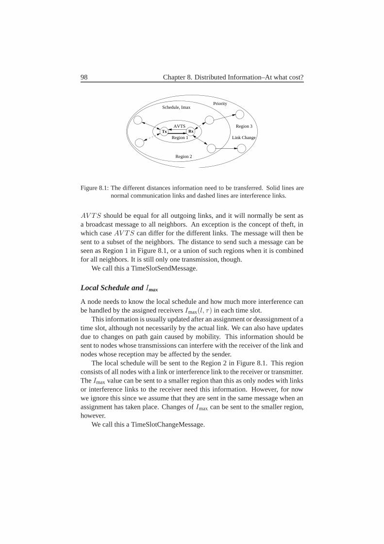
98 Chapter 8. Distributed Information–At what cost?
Tx RxAVTS
Schedule, ImaxPriority
Link Change
Region 3
Region 2
Region 1
Figure 8.1: The different distances information need to be transferred. Solid lines arenormal communication links and dashed lines are interference links.
AV TS should be equal for all outgoing links, and it will normally be sent asa broadcast message to all neighbors. An exception is the concept of theft, inwhich case AV TS can differ for the different links. The message will then besent to a subset of the neighbors. The distance to send such a message can beseen as Region 1 in Figure 8.1, or a union of such regions when it is combinedfor all neighbors. It is still only one transmission, though.
We call this a TimeSlotSendMessage.
Local Schedule and Imax
A node needs to know the local schedule and how much more interference canbe handled by the assigned receivers Imax(l, τ) in each time slot.
This information is usually updated after an assignment or deassignment of atime slot, although not necessarily by the actual link. We can also have updatesdue to changes on path gain caused by mobility. This information should besent to nodes whose transmissions can interfere with the receiver of the link andnodes whose reception may be affected by the sender.
The local schedule will be sent to the Region 2 in Figure 8.1. This regionconsists of all nodes with a link or interference link to the receiver or transmitter.The Imax value can be sent to a smaller region than this as only nodes with linksor interference links to the receiver need this information. However, for nowwe ignore this since we assume that they are sent in the same message when anassignment has taken place. Changes of Imax can be sent to the smaller region,however.
We call this a TimeSlotChangeMessage.
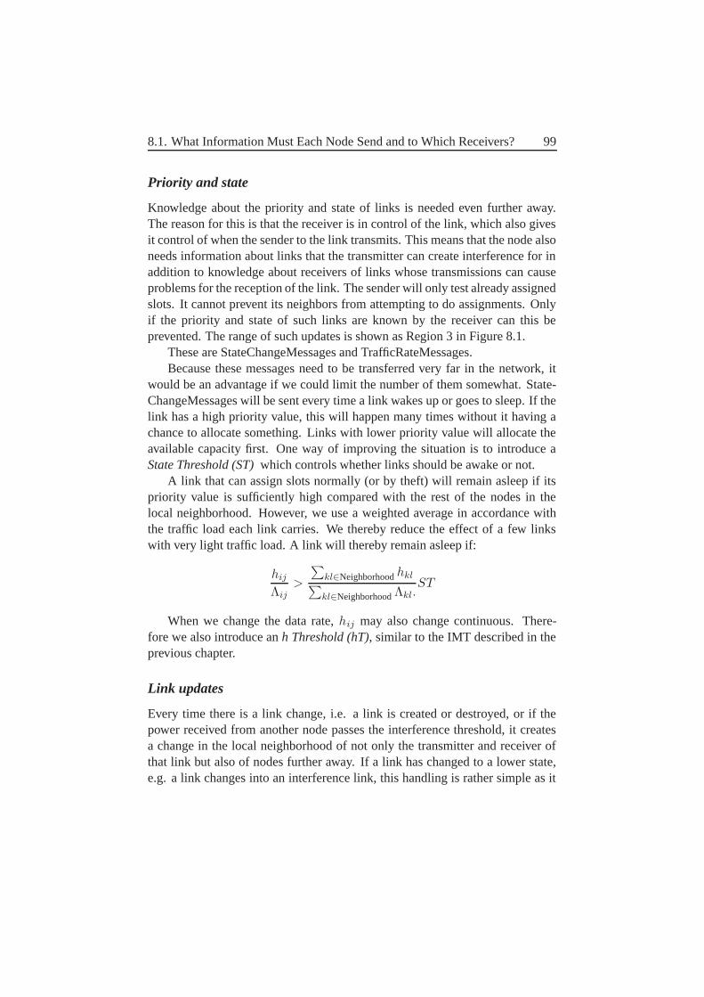
8.1. What Information Must Each Node Send and to Which Receivers? 99
Priority and state
Knowledge about the priority and state of links is needed even further away.The reason for this is that the receiver is in control of the link, which also givesit control of when the sender to the link transmits. This means that the node alsoneeds information about links that the transmitter can create interference for inaddition to knowledge about receivers of links whose transmissions can causeproblems for the reception of the link. The sender will only test already assignedslots. It cannot prevent its neighbors from attempting to do assignments. Onlyif the priority and state of such links are known by the receiver can this beprevented. The range of such updates is shown as Region 3 in Figure 8.1.
These are StateChangeMessages and TrafficRateMessages.Because these messages need to be transferred very far in the network, it
would be an advantage if we could limit the number of them somewhat. State-ChangeMessages will be sent every time a link wakes up or goes to sleep. If thelink has a high priority value, this will happen many times without it having achance to allocate something. Links with lower priority value will allocate theavailable capacity first. One way of improving the situation is to introduce aState Threshold (ST) which controls whether links should be awake or not.
A link that can assign slots normally (or by theft) will remain asleep if itspriority value is sufficiently high compared with the rest of the nodes in thelocal neighborhood. However, we use a weighted average in accordance withthe traffic load each link carries. We thereby reduce the effect of a few linkswith very light traffic load. A link will thereby remain asleep if:
hij
Λij>
∑kl∈Neighborhood hkl∑kl∈Neighborhood Λkl.
ST
When we change the data rate, hij may also change continuous. There-fore we also introduce an h Threshold (hT), similar to the IMT described in theprevious chapter.
Link updates
Every time there is a link change, i.e. a link is created or destroyed, or if thepower received from another node passes the interference threshold, it createsa change in the local neighborhood of not only the transmitter and receiver ofthat link but also of nodes further away. If a link has changed to a lower state,e.g. a link changes into an interference link, this handling is rather simple as it
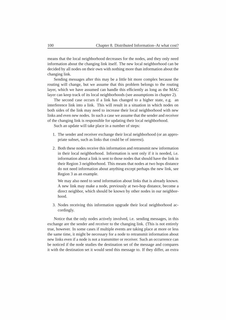
100 Chapter 8. Distributed Information–At what cost?
means that the local neighborhood decreases for the nodes, and they only needinformation about the changing link itself. The new local neighborhood can bedecided by all nodes on their own with nothing more than information about thechanging link.
Sending messages after this may be a little bit more complex because therouting will change, but we assume that this problem belongs to the routinglayer, which we have assumed can handle this efficiently as long as the MAClayer can keep track of its local neighborhoods (see assumptions in chapter 2).
The second case occurs if a link has changed to a higher state, e.g. aninterference link into a link. This will result in a situation in which nodes onboth sides of the link may need to increase their local neighborhood with newlinks and even new nodes. In such a case we assume that the sender and receiverof the changing link is responsible for updating their local neighborhood.
Such an update will take place in a number of steps:
1. The sender and receiver exchange their local neighborhood (or an appro-priate subset, such as links that could be of interest).
2. Both these nodes receive this information and retransmit new informationin their local neighborhood. Information is sent only if it is needed, i.e.information about a link is sent to those nodes that should have the link intheir Region 3 neighborhood. This means that nodes at two hops distancedo not need information about anything except perhaps the new link, seeRegion 3 as an example.
We may also need to send information about links that is already known.A new link may make a node, previously at two-hop distance, become adirect neighbor, which should be known by other nodes in our neighbor-hood.
3. Nodes receiving this information upgrade their local neighborhood ac-cordingly.
Notice that the only nodes actively involved, i.e. sending messages, in thisexchange are the sender and receiver to the changing link. (This is not entirelytrue, however. In some cases if multiple events are taking place at more or lessthe same time, it might be necessary for a node to retransmit information aboutnew links even if a node is not a transmitter or receiver. Such an occurrence canbe noticed if the node studies the destination set of the message and comparesit with the destination set it would send this message to. If they differ, an extra
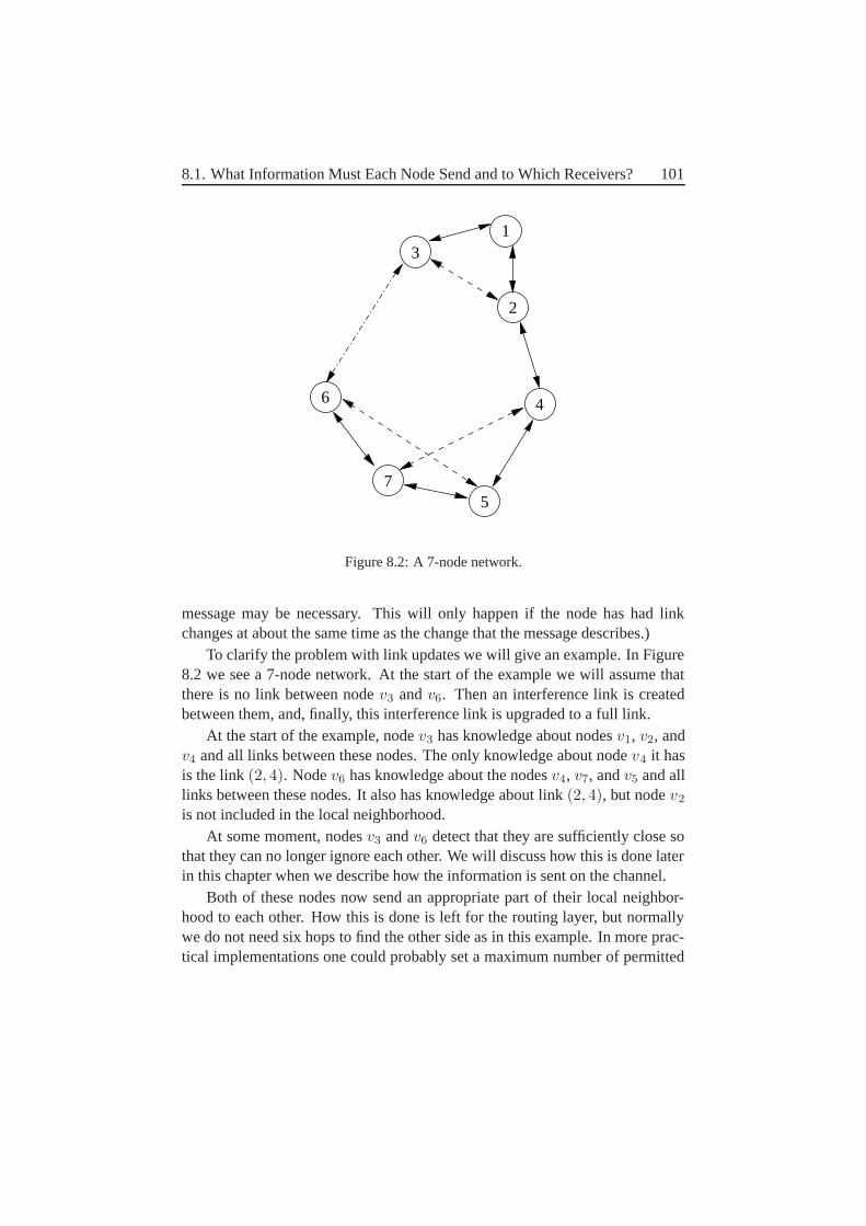
8.1. What Information Must Each Node Send and to Which Receivers? 101
31
2
4
75
6
Figure 8.2: A 7-node network.
message may be necessary. This will only happen if the node has had linkchanges at about the same time as the change that the message describes.)
To clarify the problem with link updates we will give an example. In Figure8.2 we see a 7-node network. At the start of the example we will assume thatthere is no link between node v3 and v6. Then an interference link is createdbetween them, and, finally, this interference link is upgraded to a full link.
At the start of the example, node v3 has knowledge about nodes v1, v2, andv4 and all links between these nodes. The only knowledge about node v4 it hasis the link (2, 4). Node v6 has knowledge about the nodes v4, v7, and v5 and alllinks between these nodes. It also has knowledge about link (2, 4), but node v2
is not included in the local neighborhood.At some moment, nodes v3 and v6 detect that they are sufficiently close so
that they can no longer ignore each other. We will discuss how this is done laterin this chapter when we describe how the information is sent on the channel.
Both of these nodes now send an appropriate part of their local neighbor-hood to each other. How this is done is left for the routing layer, but normallywe do not need six hops to find the other side as in this example. In more prac-tical implementations one could probably set a maximum number of permitted
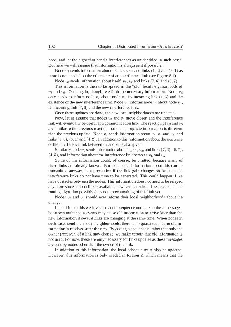
102 Chapter 8. Distributed Information–At what cost?
hops, and let the algorithm handle interferences as unidentified in such cases.But here we will assume that information is always sent if possible.
Node v3 sends information about itself, v3, v1 and links (1, 3) and (3, 1) asmore is not needed on the other side of an interference link (see Figure 8.1).
Node v6 sends information about itself, v6, v7 and links (7, 6) and (6, 7).This information is then to be spread in the “old” local neighborhoods of
v3 and v6. Once again, though, we limit the necessary information. Node v6
only needs to inform node v7 about node v3, its incoming link (1, 3) and theexistence of the new interference link. Node v3 informs node v1 about node v6,its incoming link (7, 6) and the new interference link.
Once these updates are done, the new local neighborhoods are updated.Now, let us assume that nodes v3 and v6 move closer, and the interference
link will eventually be useful as a communication link. The reaction of v3 and v6
are similar to the previous reaction, but the appropriate information is differentthan the previous update. Node v3 sends information about v3, v1 and v2, andlinks (1, 3), (3, 1) and (4, 2). In addition to this, information about the existenceof the interference link between v3 and v2 is also given.
Similarly, node v6 sends information about v6, v7, v5, and links (7, 6), (6, 7),(4, 5), and information about the interference link between v6 and v5.
Some of this information could, of course, be omitted, because many ofthese links are already known. But to be safe, information about this can betransmitted anyway, as a precaution if the link gain changes so fast that theinterference links do not have time to be generated. This could happen if wehave obstacles between the nodes. This information does not need to be relayedany more since a direct link is available, however, care should be taken since therouting algorithm possibly does not know anything of this link yet.
Nodes v3 and v6 should now inform their local neighborhoods about thechange.
In addition to this we have also added sequence numbers to these messages,because simultaneous events may cause old information to arrive later than thenew information if several links are changing at the same time. When nodes insuch cases send their local neighborhoods, there is no guarantee that no old in-formation is received after the new. By adding a sequence number that only theowner (receiver) of a link may change, we make certain that old information isnot used. For now, these are only necessary for links updates as these messagesare sent by nodes other than the owner of the link.
In addition to this information, the local schedule must also be updated.However, this information is only needed in Region 2, which means that the
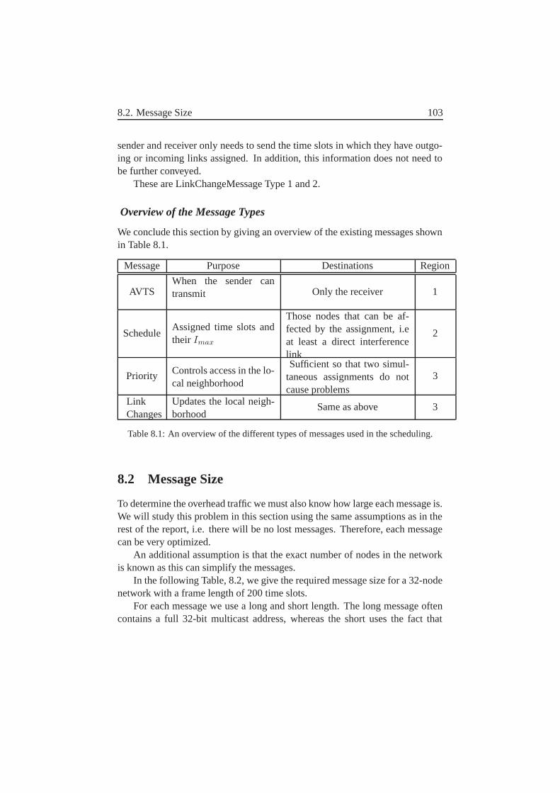
8.2. Message Size 103
sender and receiver only needs to send the time slots in which they have outgo-ing or incoming links assigned. In addition, this information does not need tobe further conveyed.
These are LinkChangeMessage Type 1 and 2.
Overview of the Message Types
We conclude this section by giving an overview of the existing messages shownin Table 8.1.
Message Purpose Destinations Region
AVTSWhen the sender cantransmit Only the receiver 1
ScheduleAssigned time slots andtheir Imax
Those nodes that can be af-fected by the assignment, i.eat least a direct interferencelink
2
Priority Controls access in the lo-cal neighborhood
Sufficient so that two simul-taneous assignments do notcause problems
3
LinkChanges
Updates the local neigh-borhood
Same as above 3
Table 8.1: An overview of the different types of messages used in the scheduling.
8.2 Message Size
To determine the overhead traffic we must also know how large each message is.We will study this problem in this section using the same assumptions as in therest of the report, i.e. there will be no lost messages. Therefore, each messagecan be very optimized.
An additional assumption is that the exact number of nodes in the networkis known as this can simplify the messages.
In the following Table, 8.2, we give the required message size for a 32-nodenetwork with a frame length of 200 time slots.
For each message we use a long and short length. The long message oftencontains a full 32-bit multicast address, whereas the short uses the fact that
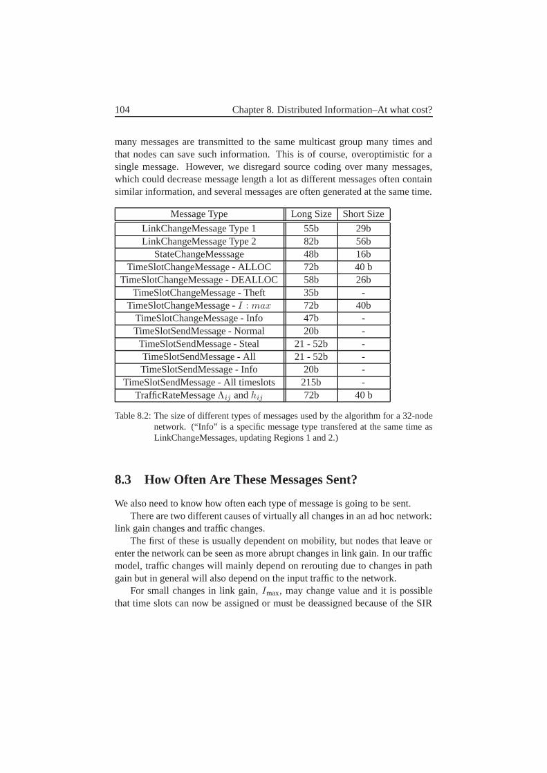
104 Chapter 8. Distributed Information–At what cost?
many messages are transmitted to the same multicast group many times andthat nodes can save such information. This is of course, overoptimistic for asingle message. However, we disregard source coding over many messages,which could decrease message length a lot as different messages often containsimilar information, and several messages are often generated at the same time.
Message Type Long Size Short Size
LinkChangeMessage Type 1 55b 29bLinkChangeMessage Type 2 82b 56b
StateChangeMesssage 48b 16bTimeSlotChangeMessage - ALLOC 72b 40 b
TimeSlotChangeMessage - DEALLOC 58b 26bTimeSlotChangeMessage - Theft 35b -
TimeSlotChangeMessage - I : max 72b 40bTimeSlotChangeMessage - Info 47b -TimeSlotSendMessage - Normal 20b -
TimeSlotSendMessage - Steal 21 - 52b -TimeSlotSendMessage - All 21 - 52b -TimeSlotSendMessage - Info 20b -
TimeSlotSendMessage - All timeslots 215b -TrafficRateMessage Λij and hij 72b 40 b
Table 8.2: The size of different types of messages used by the algorithm for a 32-nodenetwork. (“Info” is a specific message type transfered at the same time asLinkChangeMessages, updating Regions 1 and 2.)
8.3 How Often Are These Messages Sent?
We also need to know how often each type of message is going to be sent.There are two different causes of virtually all changes in an ad hoc network:
link gain changes and traffic changes.The first of these is usually dependent on mobility, but nodes that leave or
enter the network can be seen as more abrupt changes in link gain. In our trafficmodel, traffic changes will mainly depend on rerouting due to changes in pathgain but in general will also depend on the input traffic to the network.
For small changes in link gain, Imax, may change value and it is possiblethat time slots can now be assigned or must be deassigned because of the SIR
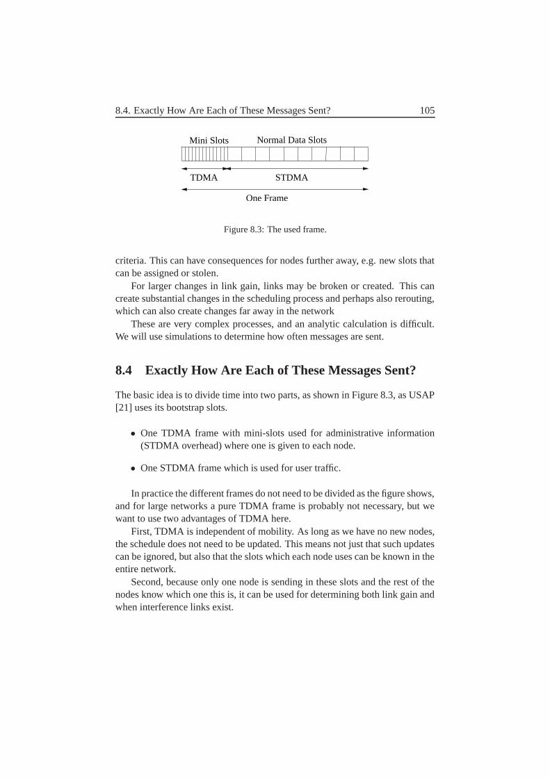
8.4. Exactly How Are Each of These Messages Sent? 105
Normal Data SlotsMini Slots
One Frame
TDMA STDMA
Figure 8.3: The used frame.
criteria. This can have consequences for nodes further away, e.g. new slots thatcan be assigned or stolen.
For larger changes in link gain, links may be broken or created. This cancreate substantial changes in the scheduling process and perhaps also rerouting,which can also create changes far away in the network
These are very complex processes, and an analytic calculation is difficult.We will use simulations to determine how often messages are sent.
8.4 Exactly How Are Each of These Messages Sent?
The basic idea is to divide time into two parts, as shown in Figure 8.3, as USAP[21] uses its bootstrap slots.
• One TDMA frame with mini-slots used for administrative information(STDMA overhead) where one is given to each node.
• One STDMA frame which is used for user traffic.
In practice the different frames do not need to be divided as the figure shows,and for large networks a pure TDMA frame is probably not necessary, but wewant to use two advantages of TDMA here.
First, TDMA is independent of mobility. As long as we have no new nodes,the schedule does not need to be updated. This means not just that such updatescan be ignored, but also that the slots which each node uses can be known in theentire network.
Second, because only one node is sending in these slots and the rest of thenodes know which one this is, it can be used for determining both link gain andwhen interference links exist.
106 Chapter 8. Distributed Information–At what cost?
In a large network, a pure TDMA frame is not very efficient. We may alsohave problems with traffic adaptivity if the administrative traffic is different onthe different nodes.
In such cases we may need to change the concept somewhat, because a pureTDMA frame is inefficient. Each node should still have one mini-slot each,but we might need more slots to handle the traffic variations. Which node thatshould send in a slot could then be decided based on priority, message history,or reservations made in the pure TDMA frame. We will not go into detail aboutthis but leave an exact implementation for future work. As long as the simplifiedoverhead is a small part of the total available capacity, the real overhead shouldnot be that much larger.
As previously stated we will assume that we have no delay for these TDMAmessages and that two independent events cannot take place simultaneously.(They may if they take place at the exact same moment in time.)
The overhead cost will now be the amount of the time that needs to be mini-slots. We also assume that this part can be varied over time, because the amountof overhead traffic generated that will be generated is dependent on the size ofthe network change that occurs. Therefore we will study the average overheadas a measurement.
8.5 What Affects the Overhead?
Before we show simulation results, it might be useful to consider which networkproperties that will affect the overhead:
• Network size
The network size has a direct effect on the TDMA frame; a doublingof the network size doubles the required TDMA frame. It may also in-crease the overhead per node if the local neighborhoods increase in size.The network size is not a parameter we can control, but it will affect theperformance of the algorithm. From Chapter 6 we also know that the re-quired frame length also increases with network size. In addition to this,the required address space will be larger for a large network.
We will mainly study a 32-node network.
• Network Connectivity
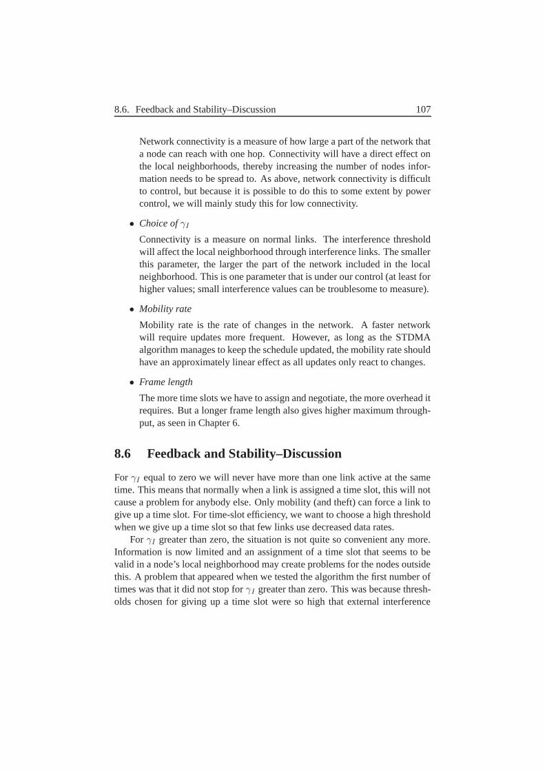
8.6. Feedback and Stability–Discussion 107
Network connectivity is a measure of how large a part of the network thata node can reach with one hop. Connectivity will have a direct effect onthe local neighborhoods, thereby increasing the number of nodes infor-mation needs to be spread to. As above, network connectivity is difficultto control, but because it is possible to do this to some extent by powercontrol, we will mainly study this for low connectivity.
• Choice of γI
Connectivity is a measure on normal links. The interference thresholdwill affect the local neighborhood through interference links. The smallerthis parameter, the larger the part of the network included in the localneighborhood. This is one parameter that is under our control (at least forhigher values; small interference values can be troublesome to measure).
• Mobility rate
Mobility rate is the rate of changes in the network. A faster networkwill require updates more frequent. However, as long as the STDMAalgorithm manages to keep the schedule updated, the mobility rate shouldhave an approximately linear effect as all updates only react to changes.
• Frame length
The more time slots we have to assign and negotiate, the more overhead itrequires. But a longer frame length also gives higher maximum through-put, as seen in Chapter 6.
8.6 Feedback and Stability–Discussion
For γI equal to zero we will never have more than one link active at the sametime. This means that normally when a link is assigned a time slot, this will notcause a problem for anybody else. Only mobility (and theft) can force a link togive up a time slot. For time-slot efficiency, we want to choose a high thresholdwhen we give up a time slot so that few links use decreased data rates.
For γI greater than zero, the situation is not quite so convenient any more.Information is now limited and an assignment of a time slot that seems to bevalid in a node’s local neighborhood may create problems for the nodes outsidethis. A problem that appeared when we tested the algorithm the first number oftimes was that it did not stop for γI greater than zero. This was because thresh-olds chosen for giving up a time slot were so high that external interference
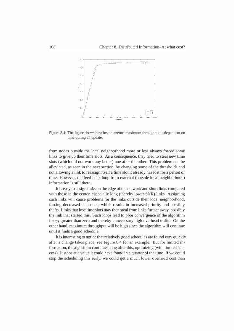
108 Chapter 8. Distributed Information–At what cost?
0 200 400 600 800 1000 1200 1400 1600 1800 20000
0.1
0.2
0.3
0.4
0.5
0.6
0.7
iterations
λ
γI=1
γI=0
Figure 8.4: The figure shows how instantaneous maximum throughput is dependent ontime during an update.
from nodes outside the local neighborhood more or less always forced somelinks to give up their time slots. As a consequence, they tried to steal new timeslots (which did not work any better) one after the other. This problem can bealleviated, as seen in the next section, by changing some of the thresholds andnot allowing a link to reassign itself a time slot it already has lost for a period oftime. However, the feed-back loop from external (outside local neighborhood)information is still there.
It is easy to assign links on the edge of the network and short links comparedwith those in the center, especially long (thereby lower SNR) links. Assigningsuch links will cause problems for the links outside their local neighborhood,forcing decreased data rates, which results in increased priority and possiblythefts. Links that lose time slots may then steal from links further away, possiblythe link that started this. Such loops lead to poor convergence of the algorithmfor γI greater than zero and thereby unnecessary high overhead traffic. On theother hand, maximum throughput will be high since the algorithm will continueuntil it finds a good schedule.
It is interesting to notice that relatively good schedules are found very quicklyafter a change takes place, see Figure 8.4 for an example. But for limited in-formation, the algorithm continues long after this, optimizing (with limited suc-cess). It stops at a value it could have found in a quarter of the time. If we couldstop the scheduling this early, we could get a much lower overhead cost than
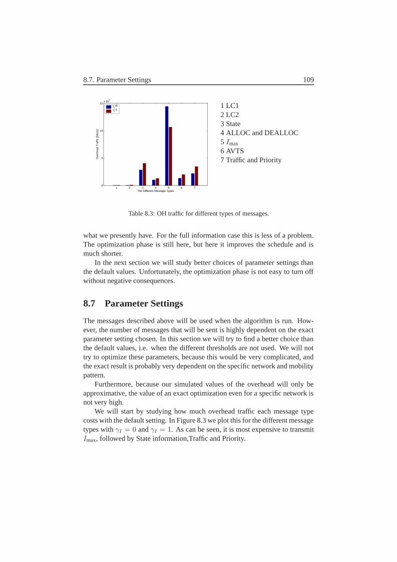
8.7. Parameter Settings 109
1 2 3 4 5 6 70
5
10
15x 10
5
Ove
rhea
d T
raffi
c [b
its/s
]
The Different Message Types
γI=0
γI=1
1 LC12 LC23 State4 ALLOC and DEALLOC5 Imax
6 AVTS7 Traffic and Priority
Table 8.3: OH traffic for different types of messages.
what we presently have. For the full information case this is less of a problem.The optimization phase is still here, but here it improves the schedule and ismuch shorter.
In the next section we will study better choices of parameter settings thanthe default values. Unfortunately, the optimization phase is not easy to turn offwithout negative consequences.
8.7 Parameter Settings
The messages described above will be used when the algorithm is run. How-ever, the number of messages that will be sent is highly dependent on the exactparameter setting chosen. In this section we will try to find a better choice thanthe default values, i.e. when the different thresholds are not used. We will nottry to optimize these parameters, because this would be very complicated, andthe exact result is probably very dependent on the specific network and mobilitypattern.
Furthermore, because our simulated values of the overhead will only beapproximative, the value of an exact optimization even for a specific network isnot very high.
We will start by studying how much overhead traffic each message typecosts with the default setting. In Figure 8.3 we plot this for the different messagetypes with γI = 0 and γI = 1. As can be seen, it is most expensive to transmitImax, followed by State information,Traffic and Priority.
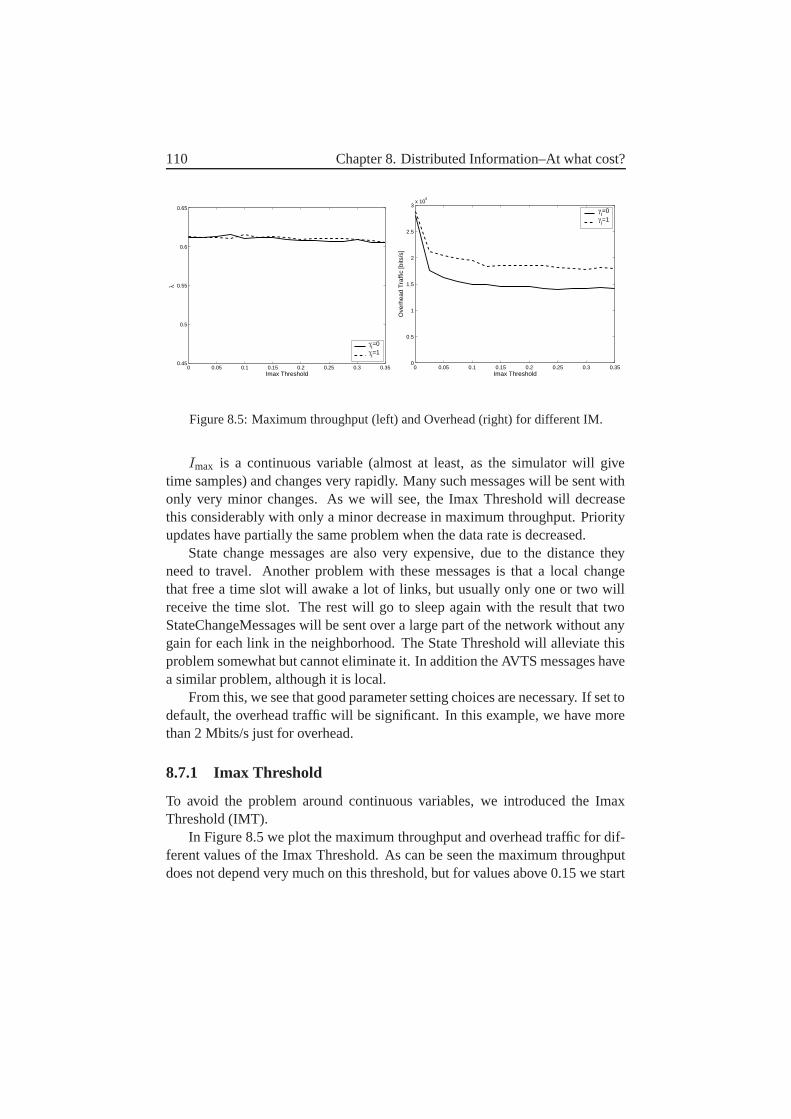
110 Chapter 8. Distributed Information–At what cost?
0 0.05 0.1 0.15 0.2 0.25 0.3 0.350.45
0.5
0.55
0.6
0.65
Imax Threshold
λ
γI=0
γI=1
0 0.05 0.1 0.15 0.2 0.25 0.3 0.350
0.5
1
1.5
2
2.5
3x 10
6
Imax Threshold
Ove
rhea
d T
raffi
c [b
its/s
]
γI=0
γI=1
Figure 8.5: Maximum throughput (left) and Overhead (right) for different IM.
Imax is a continuous variable (almost at least, as the simulator will givetime samples) and changes very rapidly. Many such messages will be sent withonly very minor changes. As we will see, the Imax Threshold will decreasethis considerably with only a minor decrease in maximum throughput. Priorityupdates have partially the same problem when the data rate is decreased.
State change messages are also very expensive, due to the distance theyneed to travel. Another problem with these messages is that a local changethat free a time slot will awake a lot of links, but usually only one or two willreceive the time slot. The rest will go to sleep again with the result that twoStateChangeMessages will be sent over a large part of the network without anygain for each link in the neighborhood. The State Threshold will alleviate thisproblem somewhat but cannot eliminate it. In addition the AVTS messages havea similar problem, although it is local.
From this, we see that good parameter setting choices are necessary. If set todefault, the overhead traffic will be significant. In this example, we have morethan 2 Mbits/s just for overhead.
8.7.1 Imax Threshold
To avoid the problem around continuous variables, we introduced the ImaxThreshold (IMT).
In Figure 8.5 we plot the maximum throughput and overhead traffic for dif-ferent values of the Imax Threshold. As can be seen the maximum throughputdoes not depend very much on this threshold, but for values above 0.15 we start
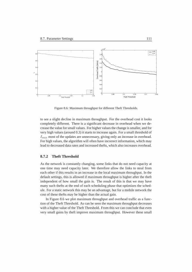
8.7. Parameter Settings 111
1 1.05 1.1 1.15 1.2 1.250
0.1
0.2
0.3
0.4
0.5
0.6
Theft Threshold
λ
γI=0
γI=1
1 1.05 1.1 1.15 1.2 1.250
0.2
0.4
0.6
0.8
1
1.2
1.4
1.6
1.8
2x 10
6
Theft ThresholdO
verh
ead
Tra
ffic
[bits
/s]
γI=0
γI=1
Figure 8.6: Maximum throughput for different Theft Thresholds.
to see a slight decline in maximum throughput. For the overhead cost it lookscompletely different. There is a significant decrease in overhead when we de-crease the value for small values. For higher values the change is smaller, and forvery high values (around 0.3) it starts to increase again. For a small threshold ofImax most of the updates are unnecessary, giving only an increase in overhead.For high values, the algorithm will often have incorrect information, which maylead to decreased data rates and increased thefts, which also increases overhead.
8.7.2 Theft Threshold
As the network is constantly changing, some links that do not need capacity atone time may need capacity later. We therefore allow the links to steal fromeach other if this results in an increase in the local maximum throughput. In thedefault settings, this is allowed if maximum throughput is higher after the theftindependent of how small the gain is. The result of this is that we may havemany such thefts at the end of each scheduling phase that optimizes the sched-ule. For a static network this may be an advantage, but for a mobile network thecost of these thefts may be higher than the actual gain.
In Figure 8.6 we plot maximum throughput and overhead traffic as a func-tion of the Theft Threshold. As can be seen the maximum throughput decreaseswith a higher value of the Theft Threshold. From this we can conclude that evenvery small gains by theft improve maximum throughput. However these small
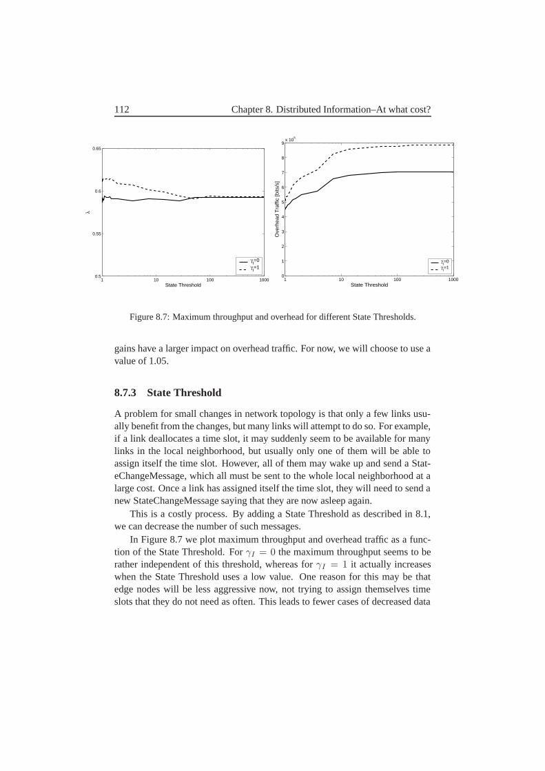
112 Chapter 8. Distributed Information–At what cost?
1 10 100 10000.5
0.55
0.6
0.65
State Threshold
λ
γI=0
γI=1
1 10 100 10000
1
2
3
4
5
6
7
8
9x 10
5
State Threshold
Ove
rhea
d T
raffi
c [b
its/s
]
γI=0
γI=1
Figure 8.7: Maximum throughput and overhead for different State Thresholds.
gains have a larger impact on overhead traffic. For now, we will choose to use avalue of 1.05.
8.7.3 State Threshold
A problem for small changes in network topology is that only a few links usu-ally benefit from the changes, but many links will attempt to do so. For example,if a link deallocates a time slot, it may suddenly seem to be available for manylinks in the local neighborhood, but usually only one of them will be able toassign itself the time slot. However, all of them may wake up and send a Stat-eChangeMessage, which all must be sent to the whole local neighborhood at alarge cost. Once a link has assigned itself the time slot, they will need to send anew StateChangeMessage saying that they are now asleep again.
This is a costly process. By adding a State Threshold as described in 8.1,we can decrease the number of such messages.
In Figure 8.7 we plot maximum throughput and overhead traffic as a func-tion of the State Threshold. For γI = 0 the maximum throughput seems to berather independent of this threshold, whereas for γI = 1 it actually increaseswhen the State Threshold uses a low value. One reason for this may be thatedge nodes will be less aggressive now, not trying to assign themselves timeslots that they do not need as often. This leads to fewer cases of decreased data
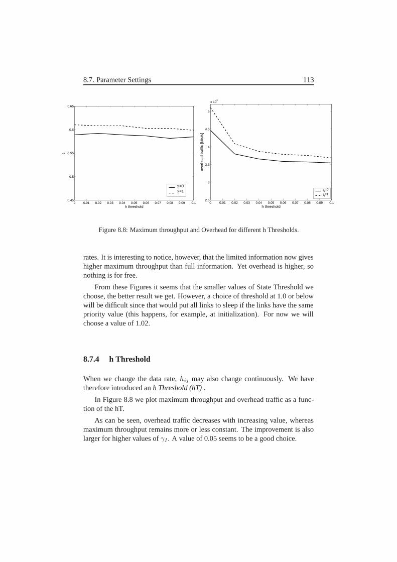
8.7. Parameter Settings 113
0 0.01 0.02 0.03 0.04 0.05 0.06 0.07 0.08 0.09 0.10.45
0.5
0.55
0.6
0.65
h threshold
λ
γI=0
γI=1
0 0.01 0.02 0.03 0.04 0.05 0.06 0.07 0.08 0.09 0.12.5
3
3.5
4
4.5
5
x 105
h thresholdov
erhe
ad tr
affic
[bits
/s]
γI=0
γI=1
Figure 8.8: Maximum throughput and Overhead for different h Thresholds.
rates. It is interesting to notice, however, that the limited information now giveshigher maximum throughput than full information. Yet overhead is higher, sonothing is for free.
From these Figures it seems that the smaller values of State Threshold wechoose, the better result we get. However, a choice of threshold at 1.0 or belowwill be difficult since that would put all links to sleep if the links have the samepriority value (this happens, for example, at initialization). For now we willchoose a value of 1.02.
8.7.4 h Threshold
When we change the data rate, hij may also change continuously. We havetherefore introduced an h Threshold (hT) .
In Figure 8.8 we plot maximum throughput and overhead traffic as a func-tion of the hT.
As can be seen, overhead traffic decreases with increasing value, whereasmaximum throughput remains more or less constant. The improvement is alsolarger for higher values of γI . A value of 0.05 seems to be a good choice.
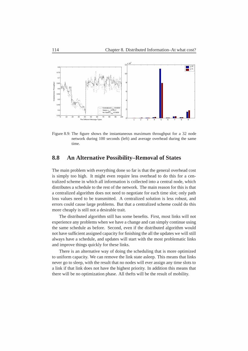
114 Chapter 8. Distributed Information–At what cost?
0 10 20 30 40 50 60 70 80 90 1000.35
0.4
0.45
0.5
0.55
0.6
0.65
0.7
0.75
0.8
The Different Message Types
Inst
anta
neou
s T
hrou
ghpu
t
Centralized γavg
=0.6034States γ
avg=0.6127
No States γavg
=0.5658
1 2 3 4 5 6 7 8 90
2
4
6
8
10
12x 10
5
γI=0
γI=1
Figure 8.9: The figure shows the instantaneous maximum throughput for a 32 nodenetwork during 100 seconds (left) and average overhead during the sametime.
8.8 An Alternative Possibility–Removal of States
The main problem with everything done so far is that the general overhead costis simply too high. It might even require less overhead to do this for a cen-tralized scheme in which all information is collected into a central node, whichdistributes a schedule to the rest of the network. The main reason for this is thata centralized algorithm does not need to negotiate for each time slot; only pathloss values need to be transmitted. A centralized solution is less robust, anderrors could cause large problems. But that a centralized scheme could do thismore cheaply is still not a desirable trait.
The distributed algorithm still has some benefits. First, most links will notexperience any problems when we have a change and can simply continue usingthe same schedule as before. Second, even if the distributed algorithm wouldnot have sufficient assigned capacity for finishing the all the updates we will stillalways have a schedule, and updates will start with the most problematic linksand improve things quickly for these links.
There is an alternative way of doing the scheduling that is more optimizedto uniform capacity. We can remove the link state asleep. This means that linksnever go to sleep, with the result that no nodes will ever assign any time slots toa link if that link does not have the highest priority. In addition this means thatthere will be no optimization phase. All thefts will be the result of mobility.
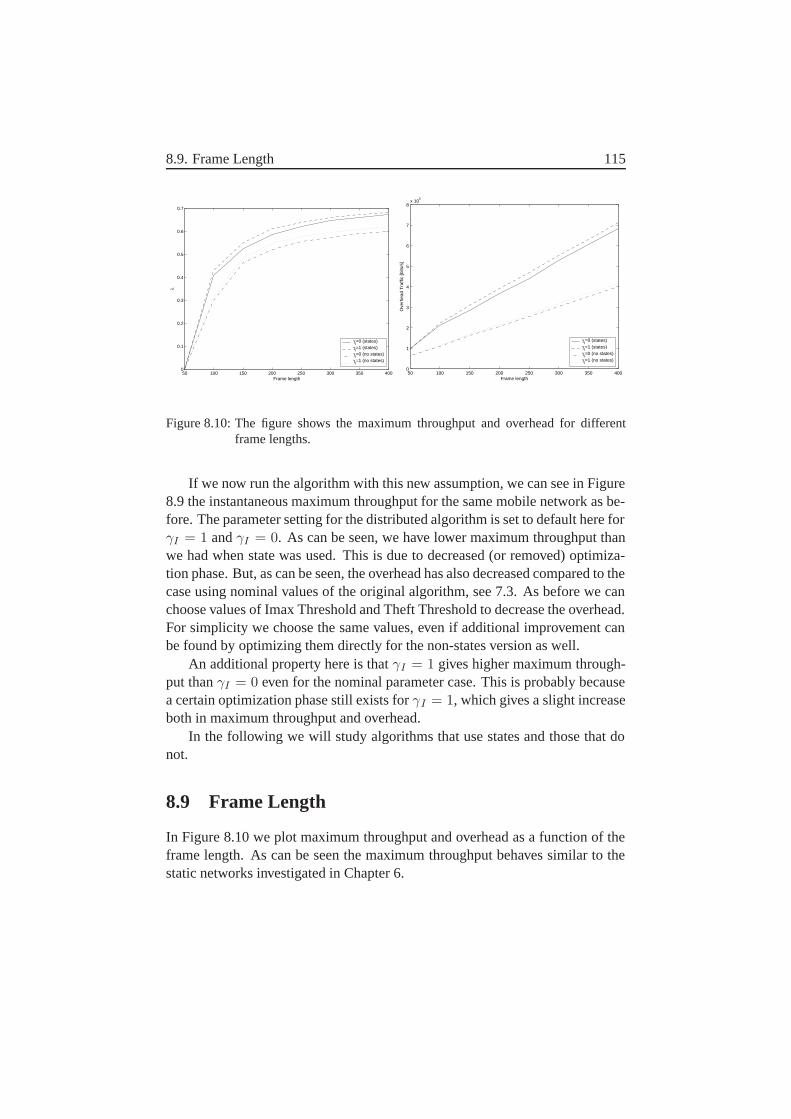
8.9. Frame Length 115
50 100 150 200 250 300 350 4000
0.1
0.2
0.3
0.4
0.5
0.6
0.7
Frame length
λ
γI=0 (states)
γI=1 (states)
γI=0 (no states)
γI=1 (no states)
50 100 150 200 250 300 350 4000
1
2
3
4
5
6
7
8x 10
5
Frame length
Ove
rhea
d T
raffi
c [b
its/s
]
γI=0 (states)
γI=1 (states)
γI=0 (no states)
γI=1 (no states)
Figure 8.10: The figure shows the maximum throughput and overhead for differentframe lengths.
If we now run the algorithm with this new assumption, we can see in Figure8.9 the instantaneous maximum throughput for the same mobile network as be-fore. The parameter setting for the distributed algorithm is set to default here forγI = 1 and γI = 0. As can be seen, we have lower maximum throughput thanwe had when state was used. This is due to decreased (or removed) optimiza-tion phase. But, as can be seen, the overhead has also decreased compared to thecase using nominal values of the original algorithm, see 7.3. As before we canchoose values of Imax Threshold and Theft Threshold to decrease the overhead.For simplicity we choose the same values, even if additional improvement canbe found by optimizing them directly for the non-states version as well.
An additional property here is that γI = 1 gives higher maximum through-put than γI = 0 even for the nominal parameter case. This is probably becausea certain optimization phase still exists for γI = 1, which gives a slight increaseboth in maximum throughput and overhead.
In the following we will study algorithms that use states and those that donot.
8.9 Frame Length
In Figure 8.10 we plot maximum throughput and overhead as a function of theframe length. As can be seen the maximum throughput behaves similar to thestatic networks investigated in Chapter 6.
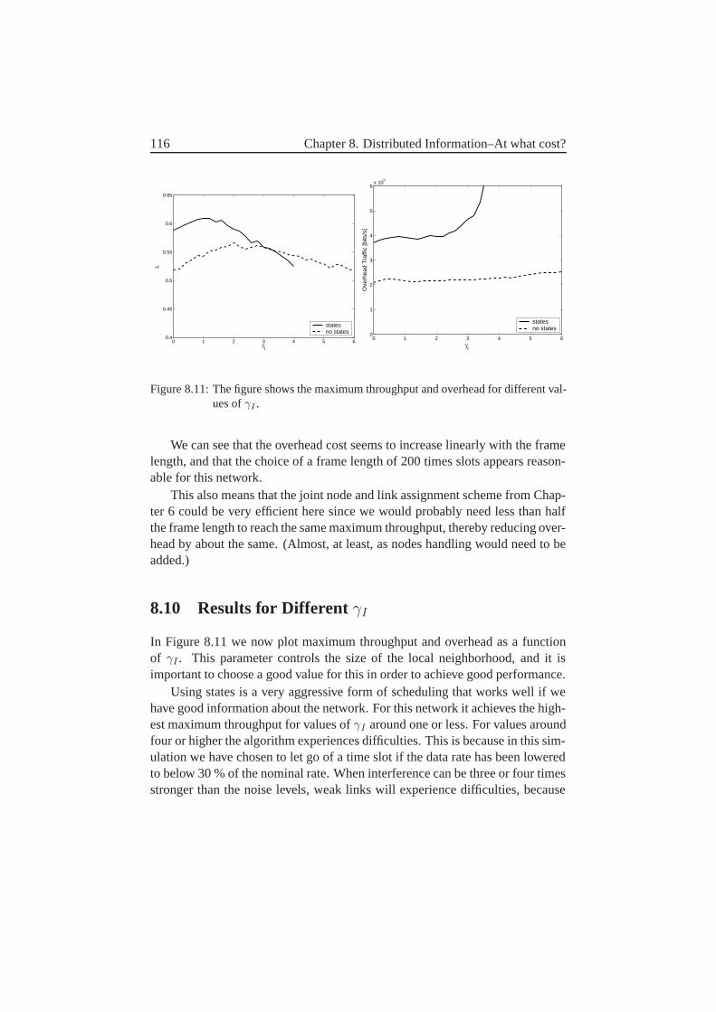
116 Chapter 8. Distributed Information–At what cost?
0 1 2 3 4 5 60.4
0.45
0.5
0.55
0.6
0.65
γI
λ
statesno states
0 1 2 3 4 5 60
1
2
3
4
5
6x 10
5
γI
Ove
rhea
d T
raffi
c [b
its/s
]
statesno states
Figure 8.11: The figure shows the maximum throughput and overhead for different val-ues of γI .
We can see that the overhead cost seems to increase linearly with the framelength, and that the choice of a frame length of 200 times slots appears reason-able for this network.
This also means that the joint node and link assignment scheme from Chap-ter 6 could be very efficient here since we would probably need less than halfthe frame length to reach the same maximum throughput, thereby reducing over-head by about the same. (Almost, at least, as nodes handling would need to beadded.)
8.10 Results for Different γI
In Figure 8.11 we now plot maximum throughput and overhead as a functionof γI . This parameter controls the size of the local neighborhood, and it isimportant to choose a good value for this in order to achieve good performance.
Using states is a very aggressive form of scheduling that works well if wehave good information about the network. For this network it achieves the high-est maximum throughput for values of γI around one or less. For values aroundfour or higher the algorithm experiences difficulties. This is because in this sim-ulation we have chosen to let go of a time slot if the data rate has been loweredto below 30 % of the nominal rate. When interference can be three or four timesstronger than the noise levels, weak links will experience difficulties, because
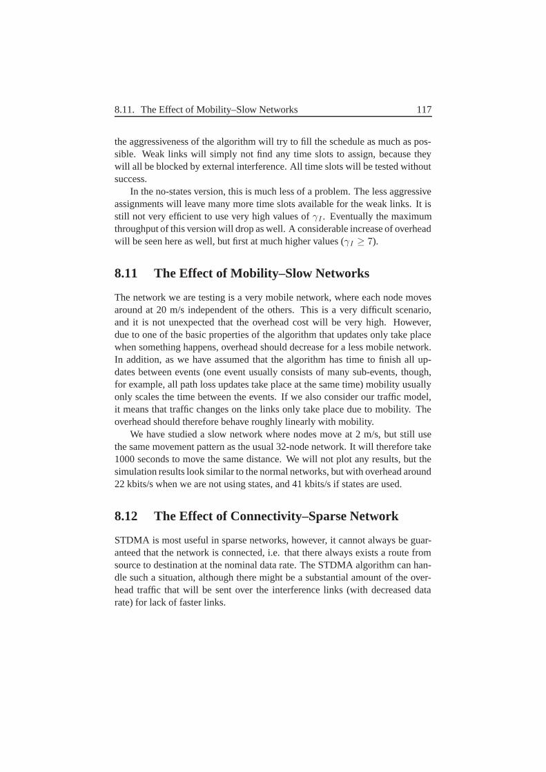
8.11. The Effect of Mobility–Slow Networks 117
the aggressiveness of the algorithm will try to fill the schedule as much as pos-sible. Weak links will simply not find any time slots to assign, because theywill all be blocked by external interference. All time slots will be tested withoutsuccess.
In the no-states version, this is much less of a problem. The less aggressiveassignments will leave many more time slots available for the weak links. It isstill not very efficient to use very high values of γI . Eventually the maximumthroughput of this version will drop as well. A considerable increase of overheadwill be seen here as well, but first at much higher values (γI ≥ 7).
8.11 The Effect of Mobility–Slow Networks
The network we are testing is a very mobile network, where each node movesaround at 20 m/s independent of the others. This is a very difficult scenario,and it is not unexpected that the overhead cost will be very high. However,due to one of the basic properties of the algorithm that updates only take placewhen something happens, overhead should decrease for a less mobile network.In addition, as we have assumed that the algorithm has time to finish all up-dates between events (one event usually consists of many sub-events, though,for example, all path loss updates take place at the same time) mobility usuallyonly scales the time between the events. If we also consider our traffic model,it means that traffic changes on the links only take place due to mobility. Theoverhead should therefore behave roughly linearly with mobility.
We have studied a slow network where nodes move at 2 m/s, but still usethe same movement pattern as the usual 32-node network. It will therefore take1000 seconds to move the same distance. We will not plot any results, but thesimulation results look similar to the normal networks, but with overhead around22 kbits/s when we are not using states, and 41 kbits/s if states are used.
8.12 The Effect of Connectivity–Sparse Network
STDMA is most useful in sparse networks, however, it cannot always be guar-anteed that the network is connected, i.e. that there always exists a route fromsource to destination at the nominal data rate. The STDMA algorithm can han-dle such a situation, although there might be a substantial amount of the over-head traffic that will be sent over the interference links (with decreased datarate) for lack of faster links.
118 Chapter 8. Distributed Information–At what cost?
0 1 2 3 4 5 60.4
0.42
0.44
0.46
0.48
0.5
0.52
0.54
0.56
0.58
γI
λ
statesno states
0 1 2 3 4 5 60
0.5
1
1.5
2
2.5
3
3.5
4
4.5
5x 10
5
γI
Ove
rhea
d T
raffi
c [b
its/s
]
statesno states
Figure 8.12: The figure shows the maximum throughput and overhead for the sparsenetwork.
We will therefore study a partly unconnected 32-node network, with an aver-age of 95 percent possible paths. One of the main benefits of the sparse networkis the fewer number of links than the previously tested network. This will allowus to use a shorter frame length, 150 time slots.
In Figure 8.12 we plot the maximum throughput for the sparse network as afunction of γI .
The curves look similar to those for the normal network. However, thereis one significant difference: The cost of full information is now much moreexpensive. It is much more costly to send information to all nodes in a non-connected network because this requires decreased rates and the use of interfer-ence links. This suggests that full information may also be very expensive ifthe network size increases and the number of hops in the network increases. Avalue of γI equal to one or higher works well for the version with states, evenhigher for no-states.
In addition, the frame length is reduced by a quarter, as is the overheadtraffic. The requirement for a short frame length is obvious.
8.13 Comparison to Centralized Scheduling
As a final comparison we once again make a comparison to what maximumthroughput that could be achievable with a centralized algorithm. In Figure 8.13(left) we show the instantaneous maximum throughput for a mobile network for
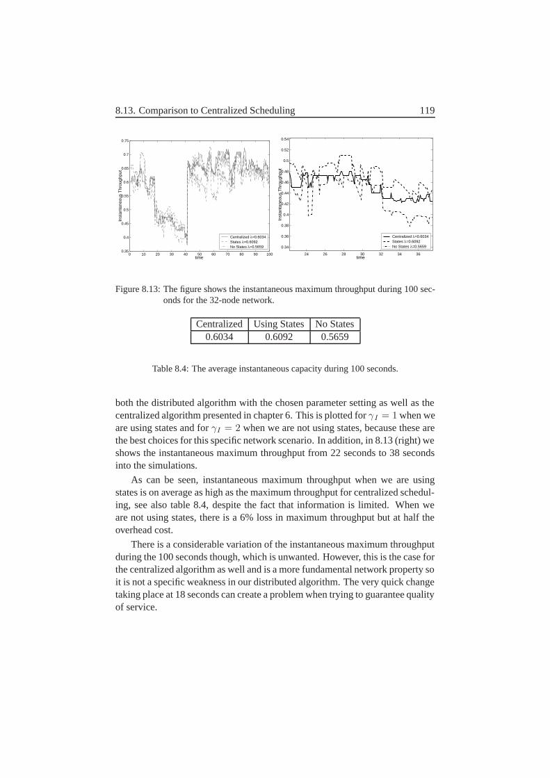
8.13. Comparison to Centralized Scheduling 119
0 10 20 30 40 50 60 70 80 90 1000.35
0.4
0.45
0.5
0.55
0.6
0.65
0.7
0.75
time
Inst
anta
neou
s T
hrou
ghpu
t
Centralized λ=0.6034States λ=0.6092No States λ=0.5659
24 26 28 30 32 34 36
0.34
0.36
0.38
0.4
0.42
0.44
0.46
0.48
0.5
0.52
0.54
time
Inst
anta
neou
s T
hrou
ghpu
t
Centralized λ=0.6034States λ=0.6092No States λ=0.5659
Figure 8.13: The figure shows the instantaneous maximum throughput during 100 sec-onds for the 32-node network.
Centralized Using States No States0.6034 0.6092 0.5659
Table 8.4: The average instantaneous capacity during 100 seconds.
both the distributed algorithm with the chosen parameter setting as well as thecentralized algorithm presented in chapter 6. This is plotted for γI = 1 when weare using states and for γI = 2 when we are not using states, because these arethe best choices for this specific network scenario. In addition, in 8.13 (right) weshows the instantaneous maximum throughput from 22 seconds to 38 secondsinto the simulations.
As can be seen, instantaneous maximum throughput when we are usingstates is on average as high as the maximum throughput for centralized schedul-ing, see also table 8.4, despite the fact that information is limited. When weare not using states, there is a 6% loss in maximum throughput but at half theoverhead cost.
There is a considerable variation of the instantaneous maximum throughputduring the 100 seconds though, which is unwanted. However, this is the case forthe centralized algorithm as well and is a more fundamental network property soit is not a specific weakness in our distributed algorithm. The very quick changetaking place at 18 seconds can create a problem when trying to guarantee qualityof service.
120 Chapter 8. Distributed Information–At what cost?
These results do not consider the cost of overhead, however, but in orderto do so we would need to consider data rates on the channel as well. If wehave a 1 Mbit/s instantaneous link data rate, the cost of 200-400 kbit/s would beconsiderable and much of the capacity would be needed just to handle overheadtraffic. On the other hand, for 10 Mbit/s or more these costs would be a smallproportion of the total available capacity.
8.14 Future Work and Improvements
A number of improvements could be added to the algorithm to make it moreefficient. One improvement is to allow nodes to assign more than one time slotat a time. This could be allowed if many time slots are available and the nodecan determine that it will receive more than one time slot for its links. This isthe case for long frame lengths and could be one way to decrease the number ofmessages sent.
Another improvement is for the nodes to keep track of the local maximumthroughput and how this changes over time. A node could use this to determinewhether the network is in the first improving phase or the optimization phase inthe end. Some minor tests on this have been performed that appears to give goodresults, but as this further increases the complexity of the algorithm simplersolutions would be preferable.
An additional way of decreasing the overhead is to attack the data rate feed-back loop by ignoring the decreased data rate from the link layer as long as thedata rate is not so low that the link should be deallocated from the time slot orthat the algorithm calculates with modified data rates, i.e. the data rate used incalculations will be somewhere between real data rate and nominal.
In addition, we need to provide an efficient solution for how to transmit theoverhead messages on the channel. A pure TDMA channel is not sufficient. Wealso need a more dynamic part that can handle the varying administrative trafficloads.
Node assignment could be implemented by turning control over to the trans-mitter instead of the receiver. A node could be assigned the time slot if all itsoutgoing links could be assigned in a time slot. This would also allow us touse joint node and link assignment, thereby reducing the need for long framelengths.
8.15. Conclusions 121
8.15 Conclusions
In this chapter we have studied how much overhead the distributed algorithmgenerated. We have also studied how different parameter settings should bechosen. Good settings are necessary to reduce overhead. But such a settingworks fairly well for the different networks we have studied.
The overhead traffic requirements can be significant, especially if we needa large frame length and the network is very mobile. For slower networks theamount of generated overhead is easily handleable. For larger, highly mobilenetworks (which also requires larger frame lengths) high link data rates will beneeded.
We have described two different approaches: using states and not usingstates.
Using states gives a much more aggressive allocations, with schedules withmaximum throughput much closer to that of a centralized algorithm but at a costof high overhead. This overhead is currently probably much higher than whatit could be, but we have not found a simple way to reduce the overhead. Withmore work, the overhead can probably be considerably decreased.
If we remove states, we get an algorithm that is much more careful in as-signing time slots, resulting in lower throughput. But overhead requirement isso much lower that the algorithm can be possibly be used for the high mobilitycase for link data with reasonable data rates.
In addition, the required overhead can probably be reduced in the future byadding joint node and link assignment as this reduces the frame length require-ment.
All problems are definitely not solved so far but this is a good start.
122 Chapter 8. Distributed Information–At what cost?
Chapter 9
Conclusions and Discussion
Adaptations on the link layer is common today. Interference-based schedulingis a tool that can bring this kind of adaptation also to higher layers in the com-munication stack. STDMA has the potential to exploit the radio channel to amuch better degree than most currently used MAC protocols.
We started by looking at the two most common assignment strategies usedfor STDMA. For unicast traffic, link assignment behaves in the ideal case betterfor high traffic loads, achieving a higher throughput. However, this comes at acost of higher delay than node assignment for low traffic loads.
To remove the inefficiencies we developed LET, which has the advantagesof both methods. LET can be added to all link schedules, thereby considerablydecreasing delay. However, as was shown these results are only valid if we havesufficient frame length, which is not certain in all cases, especially as overheadcost is proportionate to the frame length.
To really exploit the radio channel, the separate methods are not sufficient,only a combination of them can really give us the capacity we need with asufficiently short frame length.
We have also looked at the underlying network models and seen what effectsuch a choice can have on network throughput. The traditionally used graphmodel can give very poor results in many cases. The full interference model isalways best especially for large network size and low connectivity when the gainis highest. This shows that interference-based scheduling is very interesting ifmade to work.
However, the scenarios we have envisioned STDMA to work for are gen-erally mobile, even highly mobile, and even if centralized algorithms can be a
123
124 Chapter 9. Conclusions and Discussion
help in finding and investigating properties of STDMA, they are not consideredpractically useful for us. Making STDMA distributed was one of the originalgoals, specifically if we could base it on the interference-based model. This hasbeen one of the most difficult parts of the work.
Although not complete, the algorithm developed can give results close towhat a centralized algorithm can, although the overhead traffic requirementscan be significant, especially if we need a large frame length and the networkis very mobile. For slower networks the amount of generated overhead can beeasily handleable.
For larger highly mobile networks, high link data rates will be needed, butwith a very good channel utilization as a result.
Appendix A
Simulation Model
Due to the relaying of packets the statistical properties of the behavior of thenetwork is complicated, and an exact analytical analysis of the expected delayis difficult [7]. Therefore computer simulations is used in order to determine thenetwork delay. Here we give a more detailed description of the simulation setupused.
We will first describe how the networks are generated and how the basic pathloss between all nodes are calculated. Then we will describe how simulationsin order to estimate network delay and maximum throughput have been done.
A.1 Generation of networks
All static networks used in the comparison are generated in the following way;N nodes are spread out uniformly in a sample terrain consisting of mixed mead-ows and forest. The size of the area is 15kmx25km. The center frequency ischosen as 300 MHz, and antenna heights 3 m. Both communication thresholdand reliable communication threshold are set at 10dB.
In the comparisons 500 to 1000 networks of size 10, 20, 40 and 60 nodeshave been generated with different connectivity. The connectivity is varied bychanging the transmission power for a network. The transmission power is al-ways set sufficiently high so that it gives a connected network.
125
126 Chapter A. Simulation Model
Mobile Networks
The mobile network is generated by spreading 32 nodes uniformly in the sampleterrain, then each of them move randomly with a speed of 20 m/s in this terrainduring 100 seconds. This is sampled ten times a second, i.e. a path loss matrixis generated each tenth of a second.
A.2 Link Gain
An essential part of modeling an on-ground or near-ground radio network is tomodel the electromagnetic propagation characteristics due to the terrain varia-tion. A common approach is to use the basic path-loss Lb between two nodes.The most simple assumption concerning the wave propagation is that no obsta-cles appear between the transmitting and receiving antennas, and no reflectionor diffraction exist in the neighborhood of the path between the receiving andtransmitting antennas. This model is the so-called free-space assumption.
Refined assumptions of wave propagation conditions near ground includeterrain-height information and terrain-type information to estimate the basicpath-loss. See Parsons’ [69, Sec. 2.3] for an introductory description of theproblem. In the digital terrain database we have used, the height is representedas terrain-height samples at equidistant square lattice intersection points, andthe terrain type is one of maximum 256 terrain types such as fresh water, saltwater, forest, wet ground, etc. We assign electromagnetic ground constants suchas relative dielectric constant εr and conductivity σ for each terrain type, andwe also assign surface roughness for terrain types. Our database has a 50-metergrid for the terrain-height samples and a 25 meter by 25 meter terrain-type area.
All our calculations are carried out using the wave propagation computa-tions library DetVag-90 R©, [70]. Here, we use the multiple knife-edge model ofVogler [71] with five knife edges. Currently, DetVag-90 R© works with narrow-band signals, i.e., the bandwidth of the transmitted signal should be of percent-age order of the carrier frequency.
With the assumption of omnidirectional antennas, the link gain G will beequal to 1/Lb.
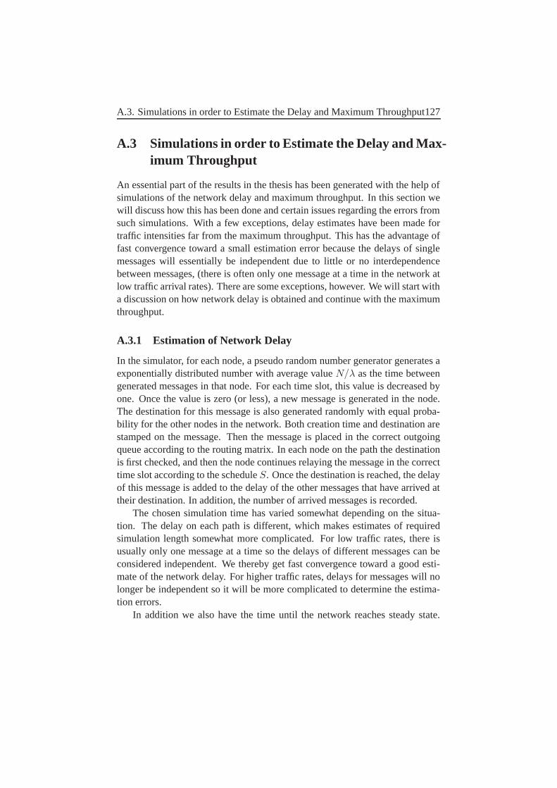
A.3. Simulations in order to Estimate the Delay and Maximum Throughput127
A.3 Simulations in order to Estimate the Delay and Max-imum Throughput
An essential part of the results in the thesis has been generated with the help ofsimulations of the network delay and maximum throughput. In this section wewill discuss how this has been done and certain issues regarding the errors fromsuch simulations. With a few exceptions, delay estimates have been made fortraffic intensities far from the maximum throughput. This has the advantage offast convergence toward a small estimation error because the delays of singlemessages will essentially be independent due to little or no interdependencebetween messages, (there is often only one message at a time in the network atlow traffic arrival rates). There are some exceptions, however. We will start witha discussion on how network delay is obtained and continue with the maximumthroughput.
A.3.1 Estimation of Network Delay
In the simulator, for each node, a pseudo random number generator generates aexponentially distributed number with average value N/λ as the time betweengenerated messages in that node. For each time slot, this value is decreased byone. Once the value is zero (or less), a new message is generated in the node.The destination for this message is also generated randomly with equal proba-bility for the other nodes in the network. Both creation time and destination arestamped on the message. Then the message is placed in the correct outgoingqueue according to the routing matrix. In each node on the path the destinationis first checked, and then the node continues relaying the message in the correcttime slot according to the schedule S. Once the destination is reached, the delayof this message is added to the delay of the other messages that have arrived attheir destination. In addition, the number of arrived messages is recorded.
The chosen simulation time has varied somewhat depending on the situa-tion. The delay on each path is different, which makes estimates of requiredsimulation length somewhat more complicated. For low traffic rates, there isusually only one message at a time so the delays of different messages can beconsidered independent. We thereby get fast convergence toward a good esti-mate of the network delay. For higher traffic rates, delays for messages will nolonger be independent so it will be more complicated to determine the estima-tion errors.
In addition we also have the time until the network reaches steady state.
128 Chapter A. Simulation Model
0 0.05 0.1 0.15 0.2 0.25 0.30
0.002
0.004
0.006
0.008
0.01
0.012
0.014
0.016
0.018
0.02
λ
std(
D)/
D
0.65 0.66 0.67 0.68 0.69 0.7 0.71 0.72 0.73 0.74 0.750
0.01
0.02
0.03
0.04
0.05
0.06
0.07
0.08
0.09
λ
std(
D)/
D
Figure A.1: The figure plots the ratio between the standard deviation of the networkdelay and network delay versus for different traffic arrival rates.
When the simulations start, the network queues will be empty. For low rates,an empty network will be very common and the time to steady state will not af-fect the simulation results very much. For high rates, this can have more effectbecause an empty network will be extremely uncommon. To avoid using mes-sages with too low delay (because they have been sent through a network withless traffic in queue than is likely) we remove the first part of the simulation, i.e.messages arriving within a certain percent of the total time are not considered atall.
The chosen simulation time has been 2000 times the frame length for lowtraffic rates. This will give approximately 2000∗0.01∗2 = 40 messages on eachpath, which should be sufficient to give an acceptable estimate of the networkdelay. We also remove the first 10 % of the simulated messages in this case. Formedium rates and high rates, the value is set to 5000 times the frame length toget a better result.
It is also important to notice that the accuracy of most simulation results isnot very important. Our main focus is more on the shape of the curves thanon the exact values of network delay for each network. We also simulate net-work delay for a large number of networks all the time, which gives us moreredundancy.
A.3. Simulations in order to Estimate the Delay and Maximum Throughput129
An example of the standard deviation of the estimated network delay
In figures A.1 we now plot an estimate of the ratio between the standard devi-ation of the network delay and network delay for different traffic arrival rates.This is done for a single 20 node network with the above parameter settings bydoing 200 separate simulations for each traffic arrival rate and from this esti-mating the standard deviation of the given results.
In the left figure this is done with low traffic arrival rates with a simulationlength of 2000 times the frame length. As can be seen, the largest deviation inthis region is in the relative order of a single percent. The error is largest at lowarrival rates, since there are much fewer messages sent through the network atthis rate.
In the right figure this is done for high traffic arrival rates with a simulationlength of 5000 times the frame length. This time the errors are larger, especiallyclose to 0.75 which is very close to the estimated maximum throughput of thisnetwork (0.757). Nevertheless, the errors are sufficiently small so that the sim-ulation results can be useful. In addition, even if errors are on the order of tensof percent close to the maximum throughput limit this will not result in so largeerrors in estimations of maximum throughput since the network delay curve isvery steep close to this value.
A.3.2 Estimation of Maximum Throughput
Maximum throughput is a much more difficult parameter to simulate becausewe want to find the largest value of the input traffic load so that we get boundeddelay. The problem with this is that to detect that delay is unbounded wouldtake infinite time to simulate, which is not possible. Instead we use the samemethod as when we estimate delay, but find which traffic load for which thenetwork delay reaches a very high value. This will not give us the real valueof the maximum throughput, but because the curve is very steep close to theasymptote, the error will be small if we choose a sufficiently large value of thenetwork delay, see for example Figure 4.2. Exactly how much we underestimatethe maximum throughput by is more difficult to say since we only know theapproximate shape of the curve.
We also have the same problem as before with reaching steady state. Thecloser to the asymptote we try to simulate network delay, the longer it takes toreach an estimate that does not rise with the simulation length. In addition, dueto the high variance and interdependence between the curves, it is difficult to
130 Chapter A. Simulation Model
ascertain that steady state has been reached.To handle this we will make partial estimates of the network delay based
on the last 1000 frame lengths and compare these with the total estimate of thenetwork delay. As long as the partial value is higher than the total value we haveprobably not reached steady state and will continue until we find a sample thatis lower or until a maximum simulation time is reached. That maximum is nowset at 30000 frame lengths, which gives approximately 30000 ∗ 2 ∗ 0.5 = 30000messages sent per path.
The maximum throughput will be found by increasing the input traffic loadλ until the delay passes the value 200 ∗ D0, where D0 is the network delay atλ = 0.01. The step size is different for different simulation. Usually it is 0.01,but in figure 3.2 the choice is 0.001.
Bibliography
[1] “FoRMA/PE Årsrapport 2000 en visionsstudie om försvarsmaktens in-satsfunktion,” Tech. Rep. FOI-R--0015--SE, Swedish Defence ResearchAgency, 2000.
[2] A. Hansson et al., “Tactical radio access networks - a comparison of adhoc and cellular network concepts,” Technical report FOI-R--0086--SE,Swedish Defence Reasearch Agency, 2001.
[3] C. Siva Ram Murthy and B.S. Manoj, Ad Hoc Wireless Networks: Ar-chitechtures and Protocols, Prentice Hall, 2004.
[4] L. Kleinrock and F. Tobagi, “Packet switching in radio channels part I –carrier sense multiple-access modes and their throughput-delay character-istics,” IEEE Trans. Commun., vol. 23, pp. 1400–1416, Dec. 1975.
[5] 1999 Edition ANSI/IEEE Std 802.11, Part 11: Wireless LAN MediumAccess Control (MAC) and Physical Layer (Phy) Specifications, Informa-tion technology– Telecommunications and information exchange betweensystems– Local and metropolitan area networks– Specific requirements–.
[6] J. Sobrinho and A. Krishnakumar, “Quality-of-service in ad hoc carriersense multiple access wireless networks,” IEEE Journal on Selected Areasof Communications, vol. 17, no. 8, pp. 1353–1368, Aug. 1999.
[7] R. Nelson and L. Kleinrock, “Spatial-TDMA: A collision-free multihopchannel access protocol,” IEEE Trans. Commun., vol. 33, no. 9, pp. 934–944, Sept. 1985.
[8] A. Ephremides and T. Truong, “Scheduling broadcasts in multihop radionetworks,” IEEE Trans. Commun., vol. 38, no. 4, pp. 456–460, Apr. 1990.
131
132 BIBLIOGRAPHY
[9] M. Huson and A. Sen, “Scheduling algorithms for packet radio networks,”in Proc. of Twelfth International Conference on Computer Communica-tions, 1995, pp. 285–290.
[10] J. Grönkvist, E. Englund, A. Hansson, and C. Jönsson, “Spatial TDMAfor multi-hop radio networks,” Scientific Report FOA-R--99-01223-504--SE, Defence Research Est., Div. of Command and Control Warfare Tech.Linköping, Sweden, 1999.
[11] O. Somarriba, Multihop Packet Radio Systems in Rough Terrain, Tech.lic.thesis, Radio Communication Systems, Department of Signals, Sensorsand Systems, Royal Institute of Technology, SE-100 44 Stockholm, Swe-den, Oct. 1995.
[12] A. Behzad and I. Rubin, “On the performance of graph-based schedul-ing algorithms for packet radio networks,” in Proc. GLOBECOM 2003,IEEE Global Telecommunications Conference, Conference Record, 2003,pp. 3432–3436.
[13] I. Chlamtac and S. Kutten, “A spatial reuse TDMA/FDMA for mobilemulti-hop radio networks,” in Proceedings of IEEE INFOCOM ’85, 1985,vol. 1, pp. 389–394.
[14] N. Funabiki and Y. Takefuji, “A parallel algorithm for broadcast schedul-ing problems in packet radio networks,” IEEE Trans. Commun., vol. 41,no. 6, pp. 828–831, June 1993.
[15] I. Cidon and M. Sidi, “Distributed assignment algorithms for multihoppacket radio network,” IEEE Trans. Comput., vol. 10, no. 38, pp. 1353–1361, Oct. 1989.
[16] F. Ali, P. Appani, J. Hammond, V. Mehta, D. Noneaker, and H. Russell,“Distributed and adapative TDMA algorithms for multiple-hop mobilenetworks,” in Proc. of IEEE MILCOM, 2002.
[17] I. Chlamtac and A. Lerner, “A link allocation protocol for mobile multi-hop radio networks,” in GLOBECOM ‘85, IEEE Global Telecommunica-tions Conference, Conference Record, 1985, vol. 1, pp. 238–242.
[18] L. Pond and V. Li, “A distributed time-slot assignment protocol for multi-hop broadcast packet radio networks,” in Proc. of IEEE MILCOM, 1989.
BIBLIOGRAPHY 133
[19] B. Hajek and G. Sasaki, “Link scheduling in polynomial time,” IEEETrans. Inform. Theory, vol. 34, no. 5, pp. 910–917, Sept. 1988.
[20] R. Liu and E. Lloyd, “A distributed protocol for adaptive link schedulingin ad-hoc networks,” in Proc. of IASTED international Conference onWireless and Optical Communications (WOC’2001), Banff, Canada, June2001, pp. 43–48.
[21] D. Young, “USAP: A unifying dynamic multichannel TDMA slot assign-ment protocol,” in Proc. of IEEE MILCOM, 1996.
[22] L. Bao and J.J. Garcia-Luna-Aceves, “Channel access scheduling in adhoc networks with unidirektional links,” in Proc of DIALM, 2001, pp.9–18.
[23] S. Ramanathan and E. Lloyd, “Scheduling algorithms for multihop radionetworks,” IEEE/ACM Trans. Networking., vol. 1, no. 2, pp. 166–177,Apr. 1993.
[24] S. Ramanathan, “A unified framework and algorithm for channel assign-ment in wireless networks,” Wireless Networks Journal, Mar 1999.
[25] E. Arikan, “Some complexity results about packet radio networks,” IEEETrans. Inform. Theory, vol. vol. IT-30, pp. 681–685, July 1984.
[26] R. Ramaswami and K. K. Parhi, “Distributed scheduling of broadcasts ina radio network,” in Proc. of INFOCOM, 1989.
[27] A. Sen and M. Huson, “A new model for scheduling packet radio net-works,” Wireless Networks, vol. 3, no. 1, pp. 71–82, Mar 1997.
[28] D. S. Stevens and M. H. Ammar, “Evaluation of slot allocation strategiesfor TDMA protocols in packet radio networks,” in Proc. of IEEE MIL-COM, 1990, vol. 2, pp. 835–839.
[29] J. Shor and T. Robertazzi, “Traffic sensitive algorithms and performancemeasures for the generation of self-organizing radio network schedules,”IEEE Trans. Commun., vol. 41, no. 1, pp. 16–21, Jan. 1993.
[30] J. Grönkvist, “Traffic controlled spatial reuse TDMA for multihop radionetworks,” in Proc. of IEEE PIMRC’98, 1998, vol. 3, pp. 1203–1207.
134 BIBLIOGRAPHY
[31] X. Ma and E. Lloyd, “An incremental algorithm for broadcast schedulingin packet radio networks,” in Proc. of IEEE MILCOM, 1998.
[32] I. Chlamtac and S. Pinter, “Distributed nodes organization algorithm forchannel access in a multihop dynamic radio network,” IEEE Trans. Com-put., vol. 36, no. 6, pp. 728–737, June 1987.
[33] L. Bao and J.J. Garcia-Luna-Aceves, “Distributed dynamic channel ac-cess scheduling for ad hoc networks,” Journal of Parallel and DistributedComputing, Special Issue on Wireless and Mobile Ad Hoc Networking,2002.
[34] C. Zhu and M.S. Corson, “An evolutionary-TDMA scheduling protocol(E-TDMA) for mobile ad hoc networks,” Tech. Rep. CSHCN TR 98-14,Center for Satellite and Hybrid Networks, University of Maryland, 1998,http://www.isr.umd.edu/CSHCN.
[35] R. Bittel et al., “Soldier phone: An innovative approach to wireless multi-media communications,” in Proc. of IEEE MILCOM, 1998.
[36] D. Young, “USAP multiple access: Dynamic resource allocation for mo-bile multichannel wireless networking,” in Proc. of IEEE MILCOM, 1999.
[37] C. Zhu and M.S. Corson, “A new protocol for scheduling TDMA trans-missions in mobile ad hoc networks,” Tech. Rep. CSHCN TR 2001-19,Center for Satellite and Hybrid Networks, University of Maryland, 2001,http://www.isr.umd.edu/CSHCN.
[38] I. Chlamtac and A. Lerner, “Fair algorithms for maximal link activationin multihop radio networks,” IEEE Trans. Commun., , no. 7, pp. 739–746,July 1987.
[39] L. Bao and J.J. Garcia-Luna-Aceves, “Collision-free topology-dependentchannel access scheduling,” in Proc. of IEEE MILCOM, 2000, vol. 1, pp.507–511.
[40] J. Grönkvist, “Assignment methods for spatial reuse TDMA,” in Proc. ofMobiHOC 2000, 2000.
[41] J. Grönkvist, “Novel assignment strategies for spatial reuse TDMA inwireless ad hoc networks,” Wireless Networks, 2005, accepted for publi-cation.
BIBLIOGRAPHY 135
[42] J. Grönkvist, “Node and link assignment in spatial reuse schemes,” inNordic Radio Symposium, 2001.
[43] J. Grönkvist, “Assignment methods for spatial reuse TDMA,” ScientificReport FOA-R--0142--SE, Swedish Defence Research Agency., Div. ofCommand and Control Warfare Tech. Linköping, Sweden, 2001.
[44] J. Grönkvist and A. Hansson, “Comparison between graph-based andinterference-based STDMA scheduling,” in Proc. of MobiHOC, 2001.
[45] A. Dhamdhere and J. Grönkvist, “Joint node and link assignment in anstdma network,” in Proc. of ICC, 2006.
[46] J. Grönkvist, “Distributed scheduling for mobile ad hoc networks – a novelapproach,” in Proc. of PIMRC, 2004.
[47] J. Grönkvist, “Distributed STDMA algorithms for ad hoc networks,”Scientific Report FOA-R--1059--SE, Swedish Defence Research Agency.,Div. of Command and Control. Linköping, Sweden, 2003.
[48] L. Tassiulas and A. Ephremides, “Jointly optimal routing and schedulingin packet radio networks,” IEEE Trans. Inform. Theory, vol. 38, no. 1, pp.165–168, Jan. 1992.
[49] S. Toumpis and A. Goldsmith, “Performace,optimization, and cross-layerdesign of media access protocols for wireless ad hoc networks,” in Proc.of International Conference on Communications (ICC), May 2003, pp.2234–2240.
[50] S. Toumpis and A. Goldsmith, “Capacity regions for wireless ad hoc net-works,” IEEE Trans. on Wireless Communications, vol. 2, no. 4, pp. 736–748, Jul 2003.
[51] R. L. Cruz and A. Santhanam, “Optimal routing, link scheduling andpower control in multi-hop wireless networks,” in Proc. of IEEE INFO-COM 2003, 2003.
[52] B. Radunovic and J.Y. Le Boudec, “Joint scheduling, power control androuting in symmetric, one-dimensional multi-hop wireless networks,” inProc. of WiOpt, 2003.
136 BIBLIOGRAPHY
[53] P. Björklund, P. Värbrand, and D. Yuan, “Resource optimization of spatialTDMA in ad hoc networks: A column generation approach,” in Proc. ofIEEE INFOCOM, 2003.
[54] M. Johansson and L. Xiao, “Scheduling, routing and power allocations forfairness in wireless networks,” in Proc. of VTC 2004-Spring, Milan, Italy,May 2004.
[55] J. Grönkvist, Jan Nilsson, and D. Yuan, “Throughput of optimal spatialreuse TDMA for wireless ad-hoc networks,” in Proc. of VTC 2004-Spring,Milan, Italy, May 2004.
[56] A. Behzad and I. Rubin, “Optimum intergrated link scheduling and powercontrol for ad hoc wireless network,” in Proc. IEEE international Con-ference on Wireless and mobile Computing, Networking and Communica-tions (WiMob), 2005.
[57] O. Somarriba and T. Giles, “Transmission control for spatial TDMA inwireless radio networks,” in Proc. of IEEE Conference on Mobile andWireless Communications Networks, 2002.
[58] O. Somarriba and T. Giles, “Scheduling for varaible power and rate controlfor spatial TDMA in wireless ad hoc networks,” in Proc. of the WirelessNetworking and Communications Group (WNCG), Wireless NetworkingSymposium, Oct. 2003.
[59] T. ElBatt and A. Ephremides, “Joint scheduling and power control forwireless ad-hoc networks,” in Proc. of IEEE INFOCOM 2002, 2002.
[60] K. Wang, C. Chiasserini, R. Rao, and J. Proakis, “A distributed jointscheduling and power control algorithm for multicasting in wireless adhoc networks,” in Proc. of ICC 2003, May 2003.
[61] Y. Li and A. Ephremides, “Joint scheduling, power control, and routing al-gorithm for ad-hoc wireless networks,” in Proc. of the 38th Annual HawaiiInternational Conference on System Sciences (HICSS’05), 2005.
[62] T. Sanches and J. Zander, “Adaptive antennas in spatial TDMA multihoppacket radio networks,” in RVK, 1999.
BIBLIOGRAPHY 137
[63] F. Eklöf et al, “On the performance of antenna arrays in spatial reuseTDMA ad hoc networks,” in Proc. of MILCOM’2002, IEEE Military Com-munications Conference, Conference record, 2002.
[64] L. Bao and J.J. Garcia-Luna-Aceves, “Transmission scheduling in ad hocnetworks with directional antennas,” in Proc. of MobiCom, 2002.
[65] A. Tannenbaum, Computer Networks, Fourth Edition, Prentice Hall PTR,2003.
[66] L. Kleinrock, Queuing Systems, Volume II: Computer Applications,Wiley-Interscience, 1976.
[67] C. Prohazka, “Decoupling link scheduling constraints in multihop packetradio networks,” IEEE Trans. Comput., vol. 38, no. 3, pp. 455–458, Mar1989.
[68] T. Shepard, “A channel access scheme for large dense packet radio net-works,” in ACM SIGCOMM, 1996.
[69] J. D. Parsons, The Mobile Radio Propagation Channel, Pentech Press,London, 1992.
[70] B. Asp, G. Eriksson, and P. Holm, “Detvag-90 R© — Final Report,” Sci-entific Report FOA-R--97-00566-504--SE, Defence Research Est., Div. ofCommand and Control Warfare Tech. Linköping, Sweden, Sept. 1997.
[71] L. E. Vogler, “An attenuation function for multiple knife-edge diffraction,”Radio Science, vol. 17, no. 6, pp. 1541–1546, Nov.-Dec. 1982.