Interface Crack Problems in Anisotropic Solids Analyzed … · Interface Crack Problems in...

Copyright © 2009 Tech Science Press CMES, vol.54, no.2, pp.223-252, 2009

Interface Crack Problems in Anisotropic Solids Analyzedby the MLPG

J. Sladek1, V. Sladek1, M. Wünsche2 and Ch. Zhang2

Abstract: A meshless method based on the local Petrov-Galerkin approach isproposed, to solve the interface crack problem between two dissimilar anisotropicelastic solids. Both stationary and transient mechanical and thermal loads are con-sidered for two-dimensional (2-D) problems in this paper. A Heaviside step func-tion as the test functions is applied in the weak-form to derive local integral equa-tions. Nodal points are spread on the analyzed domain, and each node is surroundedby a small circle for simplicity. The spatial variations of the displacements andtemperature are approximated by the Moving Least-Squares (MLS) scheme. Afterperforming the spatial integrations, one obtains a system of ordinary differentialequations for certain nodal unknowns. The backward finite difference method isapplied for the approximation of the diffusive term in the heat conduction equation.Then, the system of the ordinary differential equations of the second order resultingfrom the equations of motion is solved by the Houbolt finite-difference scheme asa time-stepping method.

Keywords: Meshless local Petrov-Galerkin method (MLPG), moving least-squaresapproximation, anisotropic materials, Houbolt method, backward finite differencemethod

1 Introduction

Layered or laminated composites composed of dissimilar materials are increas-ingly applied in engineering structures. Interface failure is one of the most domi-nant failure mechanisms in laminated structures. Williams (1959), Erdogan (1963,1965), England (1965), and Sih and Rice (1964, 1965) analyzed the interface crackproblems and showed that an oscillation of the stresses or overlapping of crack-faces near the crack-tip occurs although the traction-free boundary conditions are

1 Institute of Construction and Architecture, Slovak Academy of Sciences, 84503 Bratislava, Slo-vakia, [email protected]

2 Department of Civil Engineering, University of Siegen, D-57068 Siegen, Germany

224 Copyright © 2009 Tech Science Press CMES, vol.54, no.2, pp.223-252, 2009

assumed on the crack-faces. Various models, based on an assumption of the exis-tence of a small contact zone [Comninou (1977), Comninou and Schmeser (1979)],or a third material between two bonded materials ahead of the crack-tip [Atkinson(1977)], or a crack-tip with a finite opening angle [Sinclair (1980)], or no-slip zones[Mak et al. (1980)], have been proposed to avoid the above mentioned physicallyinadmissible phenomena. These models are successful in removing the oscillatorybehaviour and contribute to a better understanding of the fracture processes on abimaterial interface. Yuuki and Cho (1989) pointed out that the oscillation regioncan be ignored, since that region is extremely small and introduced a unique def-inition of the stress intensity factors to avoid the original confusion related to theanalyses of Erdogan (1963), and Rice and Sih (1965).

The solution of general boundary value problems for transient elastodynamic orthermoelastic problems in anisotropic solids requires advanced numerical methodsdue to the high mathematical complexity. Several computational methods havebeen proposed over the past years to analyze thermoelastic problems in homo-geneous materials. Shiah and Tan (1999) applied the boundary element method(BEM) for 2-D uncoupled thermoelasticity in anisotropic solids. Particular inte-gral formulations for 2-D and 3-D transient uncoupled thermoelastic analyses havebeen presented by Park and Banerjee (2002). The BEM has been successfully ap-plied also to coupled thermoelastic problems [Sladek and Sladek (1984); Dargushand Banerjee (1991); Chen and Dargush (1995); Suh and Tosaka (1989); Hosseini-Tehrani and Eslami (2000)]. Dual reciprocity BEM has been presented by Gaul etal. (2003), and Kögl and Gaul (2003). In spite of the great success of the finiteelement method (FEM) and BEM as effective numerical tools for the solution ofboundary value problems in mainly elastic solids, there is still a growing interestin the development of new advanced numerical methods. In recent years, mesh-less formulations are becoming popular due to their high adaptability and low coststo prepare input and output data in numerical analysis. The moving least squares(MLS) approximation is generally considered as one of many schemes to interpo-late discrete data with a reasonable accuracy. The order of continuity of the MLSapproximation is given by the minimum between the orders of continuity of the ba-sis functions and that of the weight function. So continuity can be tuned to a desiredvalue. In conventional discretization methods, the interpolation functions usuallyresult in a discontinuity in the secondary fields (gradients of primary fields) on theinterfaces of elements. Numerical models based on C1-continuity, such as in mesh-less methods, are expected to be more accurate than conventional discretizationtechniques in homogeneous or continuously nonhomogeneous solids. However,higher order continuous primary fields (displacements, temperature) are not ableto model jumps for secondary fields (gradients of primary fields) due to disconti-

Interface Crack Problems 225

nuities of the material coefficients on the interfaces of the joint laminates. There-fore, a special treatment for modeling discontinuities for piecewise homogeneoussolids is required in case of higher order modeling like in meshless approxima-tion [Li et al. (2003)]. A discontinous Galerkin meshfree formulation is proposedby Wang et al. (2009) to solve the potential and elasticity problems of compositematerial. The domain is partitioned into subdomains with uniform material prop-erties. The discretized meshfree particles within a subdomain are clarified as oneparticle group. Various subdomains occupied by different particle groups are thenlinked using the discontinuous Galerkin formulation where averaged interface trac-tion is constructed based on the tractions computed from the adjacent subdomains.The meshless or generalized FEM methods are also very convenient for modelingcracks. One can embed particular enrichment functions at the crack-tip so the stressintensity factors can be predicted accurately [Fleming et al, (1997)].

A variety of meshless methods has been proposed so far and some of them havebeen also applied to transient heat conduction problems [Batra et al. (2004); Sladeket al. (2003a,b, 2004a, 2005); Wu at al. (2007)] or thermoelastic problems [Sladeket al. (2001, 2006); Bobaru and Mukherjee (2003)]. They can be derived from aweak-form formulation either on the global domain or on a set of local subdomains.In the global formulation, background cells are required for the integration of theweak-form. In methods based on local weak-form formulation, no backgroundcells are required and therefore they are often referred to as truly meshless methods.The meshless local Petrov-Galerkin (MLPG) method is a fundamental base for thederivation of many meshless formulations, since the trial and the test functionscan be chosen from different functional spaces [Zhu et al. (1998); Atluri and Zhu(1998); Atluri et al. (2000); Sladek et al., (2000, 2001, 2003a,b) Sellountos et al.,(2005,2009)]. Recently, the MLPG method with a Heaviside step function as thetest functions [Atluri et al. (2003); Sladek et al., (2004b, 2006)] has been appliedto solve two-dimensional (2-D) homogeneous and continuously nonhomogeneouselastic solids. By using the MLPG, the present authors have recently analyzed3-D axisymmetric [Sladek et al. (2007)], general 3-D heat conduction [Sladeket al. (2008a)], and plate and shell problems under a thermal load [Sladek et al.(2008b,c)].

In this paper, the MLPG method is applied to solving two-dimensional transientuncoupled thermoelastic problems for an interface crack between two dissimilaranisotropic materials. Two sets of collocation nodes are assigned on both sides ofthe material interface at the same location but with different material properties.The moving least-squares (MLS) approximation is carried out separately for eachof the homogeneous domains, so that the domain of influence is truncated at theinterface. The high order continuity is kept within each homogeneous domain, but


not across the interface of the joint domains. In uncoupled thermoelasticity, thetemperature field is not influenced by the mechanical displacements. Therefore,the heat conduction equation is solved first to obtain the temperature distribution.The equations of motion are subsequently solved. In the solution procedure, nodalpoints are introduced and distributed over the analyzed domain, each of which issurrounded by a small circle for 2-D problems. The weak-form on small subdo-mains with a Heaviside step function as the test functions is applied to derive localintegral equations. After performing the spatial MLS approximation, a system ofordinary differential equations for certain nodal unknowns is obtained. The back-ward finite difference method is applied for the approximation of the diffusive termin the heat conduction equation. Then, the system of the ordinary differential equa-tions of the second order resulting from the equations of motion is solved by theHoubolt finite-difference scheme as a time-stepping method. Numerical examplesare presented and discussed to show the accuracy and the efficiency of the presentmethod.

2 Local integral equations

The governing equations of coupled linear thermoelasticity [Nowacki (1986)] takethe form

σi j, j(x,τ)+Xi(x,τ) = ρ ui(x,τ), (1)

[ki j(x)θ, j(x,τ)],i−ρ(x)c(x)θ(x,τ)−Toβi j(x)εi j(x,τ) = 0, (2)

where ui , ρ and Xi denote the acceleration of displacements, the mass density,and the body force vector, respectively. The stress field σi j is influenced not onlyby the displacement gradients in deformed elastic solids but also by the tempera-ture field distribution, since also a thermal expansion of the solids is contributingto the total strains. The temperature θ is measured from the unstrained value To,i.e. θ = T −To and εi j = 0 when T = To. Furthermore, ki j and c are the thermalconductivity tensor and the specific heat, respectively, while βi j are the materialcoefficients accounting for the interaction between the strain and the temperaturefields. A comma after a quantity represents the partial derivatives of the quantityand a dot is used for the time derivative. Note that there is a significant differencebetween the characteristic frequencies for elastic waves, fel , and heat conductionprocesses, fth, in typical solids. Hence, the time-dependent thermal loadings underthe frequency fth do not give rise to elastic waves and elastic fields can be treatedby the quasi-static approximation (with neglecting the inertia terms). Nevertheless,we consider this term in order to incorporate elastic waves into the simulations ofthe mechanical and the thermal processes under transient mechanical loadings. In


the case of thermal loadings including thermal shocks (sudden changes in thermalloading), one expects a vanishing influence of the inertia terms on the numericalresults. On the other hand, the fast time-dependent mechanical loadings under thefrequency fel cannot be followed by the heat conduction and the adiabatic approx-imation takes place, i.e. there is no heat exchange between different places in thesolids because of the absence of heat conduction. Then, the mechanical field isdescribed by the elastodynamic theory with taking the adiabatic values of the mate-rial coefficients instead of the isothermal values. However, the coupling term in theheat conduction equation of coupled thermoelasticity is usually negligible and thethermal processes can be considered separately as independent on the mechanicalfield what is the assumption of the uncoupled thermoelasticity. Then, the multi-field problem is governed by the heat conduction equation and the equations ofmotion

[ki j(x)θ, j(x,τ)],i−ρ(x)c(x)θ(x,τ)+Q(x,τ) = 0, (3)

σi j, j(x,τ)+Xi(x,τ) = ρ ui(x,τ), (4)

where only the mechanical fields are affected by the thermal ones and Q(x,τ) is abody heat source.

A static problem can be considered formally as a special case of the dynamic one,by omitting the acceleration ui(x,τ) in the equations of motion (4) and the timederivative term in equation (3). Therefore, both cases are analyzed in this papersimultaneously.

In the case of orthotropic materials, the relation between the stresses σi j and thestrains εi j including the thermal expansion, is given by the well known Duhamel-Neumann constitutive equations for the stress tensor

σi j(x,τ) = ci jklεkl(x,τ)− γi jθ(x,τ), (5)

where ci jkl are the material’s elastic constants and the stress-temperature moduliγi j can be expressed through the elastic constants and the linear thermal expansioncoefficients αkl as

γi j = ci jklαkl . (6)

For 2-D plane problems, the constitutive equation (5) is frequently written in termsof the second-order tensor of the elastic constants [Lekhnitskii (1963)]. The consti-tutive equation for orthotropic materials and plane strain problems has the follow-


ing formσ11σ22σ12

=

c11 c12 0c12 c22 00 0 c66

ε11ε222ε12

−c11 c12 c13

c12 c22 c230 0 0

α11α22α33

θ

= C

ε11ε222ε12

− γθ ,

(7)

with

γ =

c11 c12 c13c12 c22 c230 0 0

α11α22α33

=

γ11γ220

.

Equation (7) can be reduced to a simple form for isotropic materials

σi j = 2µεi j +λεkkδi j− (3λ +2µ)αθδi j (8)

with Lame’s constants λ and µ .

The following essential and natural boundary conditions are assumed for the me-chanical quantities

ui(x,τ) = ui(x,τ) on Γu,

ti(x,τ) = σi j(x,τ)n j(x) = ti(x,τ) on Γt ,

and for the thermal quantities

θ(x,τ) = θ(x,τ) on Γp,

q(x,τ) = ki jθ, j(x,τ)ni(x) = q(x,τ) on Γq,

where Γu is the part of the global boundary with prescribed displacements, whileon Γt , Γp and Γq the traction vector ti , the temperature and the heat flux q areprescribed, respectively.

Initial conditions for the mechanical and thermal quantities are prescribed as

ui(x,τ)|τ=0 = ui(x,0) and ui(x,τ)|

τ=0 = ui(x,0),

θ(x,τ)|τ=0 = θ(x,0) in Ω.


The local weak-form of the governing equations (4) can be written as [Atluri,(2004), Sladek et al. (2006)]∫Ωs

[σi j, j(x,τ)−ρ ui(x,τ)+Xi(x,τ)] u∗ik(x) dΩ = 0, (9)

where u∗ik(x) is a test function.

Applying the Gauss divergence theorem to the first integral results in∫∂Ωs

σi j(x,τ)n j(x)u∗ik(x)dΓ−∫Ωs

σi j(x,τ)u∗ik, j(x)dΩ

+∫Ωs

[−ρ ui(x,τ)+Xi(x,τ)]u∗ik(x)dΩ = 0, (10)

where ∂Ωs is the boundary of the local subdomain which consists of three parts∂Ωs = Ls ∪Γst ∪Γsu in general [Atluri, (2004)]. Here, Ls is the local boundarythat is totally inside the global domain, Γst is the part of the local boundary whichcoincides with the global traction boundary, i.e., Γst = ∂Ωs∩Γt , and similarly Γsu isthe part of the local boundary that coincides with the global displacement boundary,i.e., Γsu = ∂Ωs∩Γu.

By choosing a Heaviside step function as the test function u∗ik(x) in each subdomain

u∗ik(x) =

δik at x ∈Ωs

0 at x /∈Ωs,

the local weak-form (10) is converted into the following local boundary-domainintegral equations∫Ls+Γsu

ti(x,τ)dΓ−∫Ωs

ρ ui(x,τ)dΩ =−∫

Γst

ti(x,τ)dΓ−∫Ωs

Xi(x,τ)dΩ. (11)

Equation (11) is recognized as the overall momentum equilibrium conditions onthe subdomain Ωs. Note that the local integral equations (LIEs) (11) are validfor both homogeneous and non-homogeneous solids. Non-homogeneous materialproperties are included in eq. (11) through the elastic constants and the thermo-elastic coefficients involved in the traction components

ti(x,τ) =[ci jkl(x)uk,l(x,τ)−λi j(x)θ(x,τ)

]n j(x).


Similarly, the local weak-form of the governing equation (3) can be written as∫Ωs

[ki j(x)θ, j(x,τ)],i−ρcθ(x,τ)+Q(x,τ)

u∗(x) dΩ = 0, (12)

where u∗(x) is a test function.

Applying the Gauss divergence theorem to the local weak-form and consideringthe Heaviside step function for the test function u∗(x), one can obtain∫

Ls+Γsp

q(x,τ)dΓ−∫Ωs

ρcθ(x,τ)dΩ =−∫

Γsq

q(x,τ)dΓ−∫Ωs

Q(x,τ)dΩ. (13)

Equation (13) is similarly recognized as the energy balance condition on the sub-domain.

3 Numerical solution procedure

In the MLPG method the test and the trial functions are not necessarily from thesame functional spaces. For internal nodes, the test function is chosen as a unitstep function with its support on the local subdomain. The trial functions, on theother hand, are chosen to be the MLS approximations by using a number of nodesspreading over the domain of influence. According to the MLS [Belytschko et al.,(1996)] method, the approximation of the displacement field can be given as

uh(x) =m

∑i=1

pi(x)ai(x) = pT (x)a(x), (14)

where pT (x) = p1(x), p2(x), ...pm(x) is a vector of complete basis functions oforder m and a(x) = a1(x),a2(x), ...,am(x) is a vector of unknown parameters thatdepend on x. For example, in 2-D problems

pT (x) = 1,x1,x2 for m = 3

and

pT (x) =

1,x1,x2,x21,x1x2,x2

2

for m = 6

are linear and quadratic basis functions, respectively. The basis functions are notnecessary to be polynomials. It is convenient to introduce a r−1/2 - singularity for


the secondary fields at the crack-tip vicinity for modelling crack problems [Fleminget al., (1997)]. Then, the basis functions can be taken as the following form

pT (x)=

1,x1,x3,√

r cos(θ/2),√

r sin(θ/2),√

r sin(θ/2)sinθ ,√

r cos(θ/2)sinθ

for m = 7, (15)

where r and θ are polar coordinates with the crack-tip as the origin.

The approximated functions for the mechanical displacements and the temperaturecan be written as [Atluri, (2004)]

uh(x,τ) = ΦT (x) · u =

n

∑a=1

φa(x)ua(τ), (16)

θh(x,τ) =

n

∑a=1

φa(x)θ a(τ), (17)

where the nodal values ua(τ) = (ua1(τ), ua

2(τ))T , and θ a(τ) are fictitious parame-ters for the displacements and the temperature, respectively, and φ a(x) is the shapefunction associated with the node a. The number of nodes n used for the approxi-mation is determined by the weight function wa(x). A 4th order spline-type weightfunction is applied in the present work

wa(x) =

1−6

(da

ra

)2+8(da

ra

)3−3(da

ra

)4, 0≤ da ≤ ra

0, da ≥ ra, (18)

where da = ‖x−xa‖ and ra is the size of the support domain. The value of theradius of the support domain has been optimized on numerical experiments. Nie etal (2006) developed an efficient approach to find the optimal radius of support ofradial weight functions used in MLS approximation.

It is seen that the C1−continuity is ensured over the entire domain, and thereforethe continuity conditions of the tractions and the heat flux are satisfied. However,this highly continuous nature leads to difficulties when there is an imposed discon-tinuity in the secondary fields (strains, gradients of the temperature). Because ofthe highly continuous trial function which is at least C1, it is difficult to simulatejumps in the strain field. Krongauz and Belytschko (1998) introduced a jump shapefunction for 2-D problems. It is a trial function with a pre-imposed discontinuity inthe gradient of the function at the location of the material discontinuity in additionto the MLS approximation. This method is very tedious for curvilinear interfaces.Cordes and Moran (1996) solved also 2-D problems by using Lagrangian multi-plier. The method requires a lot of computational effort when the discontinuity isof an arbitrary geometrical shape.


Interface between two media

Medium +Medium -

circular subdomain

semi-circular subdomain for node in +

Figure 1: Modeling of material discontinuities

For 3-D problems it is much simpler to introduce double nodes in the materialdiscontinuity [Li et al. (2003)]. Two sets of collocation nodes are assigned onboth the +side and the –side of the material interface at the same location, but withdifferent material properties (Fig. 1). The MLS approximations are carried outseparately on particular sets of nodes within each of the homogeneous domains.Then, the support domains for the weights in the weighted MLS-approximationsare truncated at the interface of the two media. Therefore, the high order continuityis kept within each homogeneous part, but not across their interface. Also the localsubdomains considered around nodes should not cross the interface.

The traction vectors ti(x,τ) at a boundary point x∈ ∂Ωs are approximated in termsof the same nodal values ua(τ) and θ a(τ) as

th(x,τ) = N(x)Cn

∑a=1

Ba(x)ua(τ)−N(x)γn

∑a=1

φa(x)θ a(τ), (19)

where the matrix N(x) is related to the normal vector n(x) on ∂Ωs by

N(x) =[

n1 0 n20 n2 n1

].


The matrix Ba is represented by the gradients of the shape functions

Ba(x) =

φ a,1 00 φ a

,2φ a

,2 φ a,1

.

Similarly the heat flux q(x,τ) can be approximated by

qh(x,τ) = ki jni

n

∑a=1

φa, j(x)θ a(τ) = nT (x)K(x)

n

∑a=1

Pa(x)θ a(τ), (20)

where

K(x) =[

k11 k12k21 k22

], Pa(x) =

[φ a

,1φ a

,2

], nT (x) = (n1, n2 ).

The local integral equation for the heat conduction, eq. (13), considered at eachinterior point xi ∈Ωi

s ⊂Ω, yields the following set of equations

n

∑a=1

θa(τ)

∫∂Ωi

s

nT (x)K(x)Pa(x)dΓ−n

∑a=1

˙θ

a(τ)∫Ωi

s

ρcφa(x)dΩ =−

∫Ωi

s

Q(x,τ)dΩ.

(21)

Substituting the MLS approximations for the displacements (16) and the tractions(19) into (11) for each interior node xi, the following set of discretized LIEs for themechanical field is obtained

n

∑a=1

∫

Lis

N(x)CBa(x)dΓ

ua(τ)−ρ

∫Ωi

s

φa(x)dΩ

¨ua(τ)

−

−n

∑a=1

∫Ls+Γsu

N(x)γφa(x)dΓ

θa(τ) =

=−∫Ωi

s

X(x,τ)dΩ. (22)

The discretized displacement, traction, temperature and heat flux boundary condi-tions

n

∑a=1

φa(xb)ua(τ) = u(xb,τ) for xb ∈ ∂Ω

bs ∩ Γu = Γ

bsu, (23)


N(xb)

[C

n

∑a=1

Ba(xb)ua(τ)− γ

n

∑a=1

φa(xb)θ a(τ)

]= t(xb,τ) for xb ∈ ∂Ω

bs ∩ Γt = Γ

bst ,

(24)

n

∑a=1

φa(xb)θ a(τ) = θ(xb,τ) for xb ∈ ∂Ω

bs ∩ Γp = Γ

bsp, (25)

nT (xb)K(xb)n

∑a=1

Pa(xb)θ a(τ) = q(xb,τ) for xb ∈ ∂Ωbs ∩ Γq = Γ

bsq (26)

are considered at boundary nodes xb ∈ Γ = Γu∪Γt ∪Γp∪Γq.

On the interface ΓI of the two material media there are no boundary conditionsprescribed but we can guarantee the continuity for the displacements and the tem-perature, as well as the equilibrium for tractions and heat flux by collocating thefollowing equations at double nodes xd ∈ ∂Ωd

s ∩ΓI = ΓdI

n+

∑a=1

φa(xd)ua(τ) =

n−

∑a=1

φa(xd)ua(τ),

n+

∑a=1

φa(xd)θ a(τ) =

n−

∑a=1

φa(xd)θ a(τ),

N(xd)

[C+(xd)

n+

∑a=1

Ba(xd)ua(τ)− γ+(xd)

n+

∑a=1

φa(xd)θ a(τ)−

− C−(xd)n−

∑a=1

Ba(xd)ua(τ)+ γ−(xd)

n−

∑a=1

φa(xd)θ a(τ)

]= 0,

nT (xd)

[K+(xd)

n+

∑a=1

Pa(xd)θ a(τ)−K−(xd)n−

∑a=1

Pa(xd)θ a(τ)

]= 0, (27)

where n+ and n− are the numbers of nodes lying in the support domain in medium+ and medium -, respectively. The normal vector components in N(xd) and nT (xd)are taken in the sense of outward normal to the medium +.

The backward finite difference method is applied to the approximation of “veloci-ties”

yτ+∆τ =yτ+∆τ −yτ

∆τ, (28)

where ∆τ is the time-step.


The system of ordinary differential equations (21) and collocation equations (25)-(27) can be rearranged in such a way that all known quantities are in the secondterm of the matrix form the system equations, viz.

Ay+By = Q. (29)

Substituting eq. (28) into eq. (29) results in the following set of algebraic equationsfor the unknowns yτ+∆τ[

1∆τ

A+B]

yτ+∆τ = A1

∆τyτ+Q. (30)

Once the temperature field is computed from eq. (30), the mechanical field can bedetermined. The matrix form of the ordinary differential equations (22) and thecollocation equations (23), (24) and (27) can be written as

Lx+Kx = P. (31)

Several time integration procedures for the solution of this system of ordinary dif-ferential equations are available. In the present work, the Houbolt finite differencescheme [Houbolt (1950)] is adopted in which the acceleration u = x is expressedas

xτ+∆τ =2xτ+∆τ −5xτ +4xτ−∆τ −xτ−2∆τ

∆τ2 , (32)

where ∆τ is the time-step.

Substituting eq. (32) into eq. (31), the following system of algebraic equations isobtained for the unknowns xτ+∆τ[

2∆τ2 L+K

]xτ+∆τ = L

1∆τ2 5xτ −4xτ−∆τ +xτ−2∆τ+P. (33)

To ensure the stability, the value of the time-step has to be appropriately selectedwith respect to the material parameters (elastic wave velocities) and the time de-pendence of the boundary conditions.

4 Evaluation of stress intensity factors

For crack-tips inside a homogeneous anisotropic solid there is a well-known√

r-behaviour for the displacements at the crack-tip vicinity. This allows us to compute


the stress intensity factors (SIFs) from the asymptotic expansion of the displace-ments by an extrapolation technique. Both mode-I and mode-II SIFs can be com-puted from the following equations [Zhang (2005)]

KII(τ)KI(τ)

=

14∆

√2π

l

[H11 H12H21 H22

]∆u1(l,τ)∆u2(l,τ)

, (34)

where l is a distance from the point evaluating the crack-opening-displacements∆ui to the crack-tip and

[H11 H12H21 H22

]=

Im(

q1−q2µ1−µ2

)Im(

p2−p1µ1−µ2

)Im(

µ1q2−µ2q1µ1−µ2

)Im(

µ2q1−µ1q2µ1−µ2

) , (35)

∆ = H11H22−H12H21.

In equations (35) µα denotes the complex roots of the characteristic equation [Lekhnit-skii (1963)]

b11µ4α −2b16µ

3α +(2b12 +b66)µ

2α −2b26µα +b22 = 0, (36)

with bi j being the material compliances and

pα = b11µ2α −b16µα +b12,

qα = (b12µ2α −b26µα +b22)/µα .

For interface cracks between dissimilar anisotropic materials, the displacements atthe crack-tip vicinity show an oscillating behaviour

√r cos(ε lnr), where ε is the

bi-material constant which describes the mismatch of the elastic properties. Theabsolute value of the stress intensity factor |K| and the phase angle φ of the complexSIF are defined by Cho et al. (1992)

|K(τ)|=√

K21 +K2

2 =1+4ε2

4coshπε

√2π

l

√t221 +d2

21

d1t2− t1d2, (37)

tan φ(τ) =K2(τ)K1(τ)

=d2−d1 [∆u2(l,τ)/∆u1(l,τ)]t1 [∆u2(l,τ)/∆u1(l,τ)]− t2

, (38)

where

t21 = t2∆u1(l,τ)− t1∆u2(l,τ),


d21 = d1∆u2(l,τ)−d2∆u1(l,τ).

The constants dα , tα and the bi-material constant ε are defined in Appendix [Wün-sche et al. (2009)]. An extrapolation technique is applied to the above given equa-tions and the crack-opening displacements are computed at three different nodeson the crack-faces. Indeed, the oscillatory stress singularity at the crack-tips can betaken into account in the shape-functions in a refined approach as presented by Tanet al. (1992) and Ang et al. (1996).

5 Numerical examples

5.1 A central crack in a finite plate under a pure mechanical load

In the first example a straight central crack in a finite plate under a pure mechanicalload is analyzed. The central crack with length 2a is considered on the interfaceof two dissimilar anisotropic materials (Fig. 2). The rectangular plate is subjectedto a tensile load at the top and bottom part of the plate. The following geomet-rical values are considered in the numerical analysis:a = 0.5m, width ratio of theplatea/w = 0.4 and height ratioh/w = 1.2.

x1

x2

2a

2w

2h

cIij

cIIij

σ0

σ0

Figure 2: A central interface crack in a layered rectangular plate

To test the accuracy of the present computational method we have analyzed a crackin a homogeneous anisotropic plate corresponding to a graphite-epoxy compos-ite with a composition of 65% graphite and 35% epoxy and the following elastic


stiffness matrix

155.43 3.72 3.72 0 0 016.34 4.96 0 0 0

16.34 0 0 03.37 0 0

sym. 7.48 07.48

·109N/m2 .

A static tensile load σ0 = 1Pa and plane strain conditions are considered. Due tothe symmetry of the problem with respect to x2-axis, only a half of the strip is mod-eled. We have used 1860 (2x31x30) nodes equidistantly distributed for the MLSapproximation of the physical quantities (Fig. 3). The symmetry with respect tothe x1-axis is not utilized owing to test the computational scheme for further calcu-lations of piece-wise homogeneous media. The local subdomains are considered tobe circular with a radius rloc = 0.033m.

,

x1

x2

u = =01 2t t = =01 2t

900

,

x1

x2

u = =01 2t t = =01 2t

930

,

x1

x2t =01

u = =01 2t t = =01 2t

961

1860

931

,

x1

x2

u = =01 2t t = =01 2t

,1 31

1830

u = =01 2t t = =01 2t

t2=H(t-0)

t =01 t2=H(t-0)

Figure 3: Node distribution and boundary conditions

The crack-displacements on both crack-faces are presented in Fig. 4. One can


observe a good agreement between the MLPG and the FEM results obtained byANSYS computer code with PLANE 183 elements. The corresponding normalizedmode-I SIF KI/σ0

√πa = 1.108 is also in a good agreement with the reference value

of the handbook [Murakami (1987)]

-0.8

-0.6

-0.4

-0.2

0

0.2

0.4

0.6

0.8

0 0.1 0.2 0.3 0.4 0.5

x1 /2a

u2 (1

0-10 m

)

FEM: u+ u-MLPG: u+ u-

Figure 4: Variations of the crack-displacements with the normalized coordinatex1/2a in a homogeneous anisotropic plate subjected to a static tension

Now, we consider an inhomogeneous plate with isotropic material properties inthe upper part I with Young‘s modulus E = 100Mpa and Poisson’s ratio ν = 0.3,and orthotropic properties in the lower part II with E1 = E3 = 1 · 1011N/m2,E2 =3 ·1011N/m2, shear moduli G12 = G23 = 38.46 ·109N/m2, G13 = 115.4 ·109N/m2

and Poisson‘s ratios ν12 = ν32 = 0.1 and ν21 = ν23 = ν13 = 0.3. The correspondingelastic stiffness matrix for the orthotropic material can be obtained by the inversionof the compliance matrix as follows

116.6 46.88 39.66 0 0 0328.1 46.88 0 0 0

116.6 0 0 038.46 0 0

sym. 115.4 038.46

·109N/m2 .

The crack-displacements on both crack-faces in the inhomogeneous plate subjected


to a static tension are presented in Fig. 5. The displacement on the lower crack-face u−2 in the inhomogeneous interface crack problem is significantly reduced withrespect to the homogeneous case. It is due to the larger stiffness coefficient c22corresponding to a Young‘s moduli relation E2 = 3E1. The interface crack problem

-1.5

-1

-0.5

0

0.5

1

1.5

0 0.1 0.2 0.3 0.4 0.5

x1 /2a

u2 (1

0-9m

) homogeneous: u+ u-MLPG: interface u+MLPG: interface u-

Figure 5: Variations of the crack-displacements with the normalized coordinatex1/2a for a static tension

has been analyzed also by FEM. The numerical results for the displacement u2 arecompared in Fig. 6 and a good agreement can be observed for both crack-faces.

The same interface crack problem under an impact load with Heaviside time vari-ation is analyzed too. The mass density corresponds to graphite-epoxy compositewith ρ = 2000kgm−3 and the same material and geometrical parameters are usedfor the upper and lower parts of the specimen. The number of nodes for MLS ap-proximations is the same as in the static case and a time-step of ∆t = 7µs is chosen.

The time variation of the normalized absolute value of SIF, |K(t)|/σ0√

πa, is pre-sented in Fig. 7, where the FEM, BEM and MLPG results are compared. One canobserve a very good agreement of the numerical results.

5.2 A central crack in a finite plate under a thermal load

The geometry of the strip is given in Fig. 8 with the following values: a = 0.5,a/w = 0.4 and h/w = 1.2. On the outer boundary of the strip a thermal load T2 =


-0.8-0.6

-0.4-0.2

00.2

0.40.60.8

11.2

0 0.1 0.2 0.3 0.4 0.5

x1 /2a

u2 (1

0-9m

)

MLPG: u+ u-FEM: u+ u-

Figure 6: Variations of the crack-displacements with the normalized coordinatex1/2a for a static tension

0

0.5

1

1.5

2

2.5

0.00E+00 3.00E-04 6.00E-04 9.00E-04 1.20E-03

time t [sec]

Nor

mal

ized

SIF

FEM

BEMMLPG

Figure 7: Time variation of the normalized absolute value of SIF

θ0 = 1deg is applied. On both crack-faces a vanishing temperature is kept T1 = 0.The outer boundary is free of tractions.

Due to the symmetry of the problem with respect to x2-axis, again only a half


x1

x2

T1

T2

2a

2w

2h

Figure 8: Central crack in a finite plate with prescribed temperatures on outerboundary and crack-faces

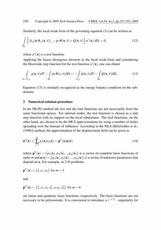
of the strip is modeled. We have used 1860 (2x31x30) nodes equidistantly dis-tributed for the MLS approximation of the physical quantities (Fig. 9). The localsubdomains are considered to be circular with a radius rloc = 0.033m. Homoge-neous material properties are selected to test the present computational method.The material constants correspond to an isotropic material with Young‘s modu-lus E = 100MPa, Poisson’s ratio ν = 0.3, mass density ρ = 7500kg/m3 , ther-mal conductivityk = 75 W/Km , thermal expansion α = 0.4 · 10−51/K and spe-cific heat conduction c = 420Wskg−1K−1. Numerical results obtained by FEMand the present MLPG are compared in Fig. 10. The stress intensity factor forthis case is equal to Kstat

I (hom .) = 2.02 · 105Pam1/2. One can observe a verygood agreement of the MLPG and the FEM results. After the numerical test ofthe accuracy we consider now the interface crack problem, where isotropic mate-rial properties in the upper part I with Young‘s modulus E = 100MPa and Pois-son’s ratio ν = 0.3, and orthotropic properties in the lower part II withE1 = E3 =1 ·1011N/m2, E2 = 3 ·1011N/m2, shear moduli G12 = G23 = 38.46 ·109N/m2 andG13 = 115.4 ·109N/m2and Poisson‘s ratios ν12 = ν32 = 0.1 and ν21 = ν23 = ν13 =0.3 are considered. The thermal conductivity k = 75 W/Km, thermal expansionα = 0.4 ·10−51/K and specific heat conduction c = 420Wskg−1K−1 are used forthe upper part I and orthotropic properties k11 = 150W/Km, k22 = 100W/Km,k12 = 0, α11 = 0.8 ·10−51/K, α22 = α33 = 0.4 ·10−51/K for part II. The variationsof the crack-opening-displacement ∆u2 along the x1-coordinate on the crack-faces


are presented in Fig. 10 for homogeneous and dissimilar materials. One can seethat the crack-opening-displacement is slightly higher for the interface crack be-tween two dissimilar materials than for the crack in a homogeneous material. Onecan again observe a very good agreement of the FEM and the MLPG results.

,

x1

x2t2=t =01

u = =01 2tθ=1t = =01 2t

θ=1

900

,

x1

x2t2=t =01

u = =01 2tθ=1t = =01 2t

θ=1

930

,

x1

x2t2=t =01

u = =01 2tθ=1t = =01 2t

θ=1

961

1860

931

,

x1

x2

u = =01 2tθ=1t = =01 2t

θ=1

t2=t =01 , θ=11 31

q=0

1830

u = =01 2tq=0 θ=1

t = =01 2t

Figure 9: Node distribution and boundary conditions

The stress intensity factor for an interface crack between two dissimilar orthotropicmaterials is a little bit higher than that one in a homogeneous material, Kstat

I (non−hom .) = 2.12 · 105Pam1/2. Figure 11 presents the variation of the temperatureahead the crack-tip at x2 = 0. The temperature variations are almost the same fora crack in a homogeneous material and an interface crack between two dissimi-lar materials. A slight difference between the temperature variations along x2 atx1/2a = 0.5 is observed on Fig. 12. Higher temperature values occur in the lowerpart of the inhomogeneous plate, where larger thermal conductivity values are con-sidered than in the upper part or in the homogeneous case.

Finally, we consider a thermal shock on the outer boundary of the finite plate witha central crack. Heaviside time variation is taken for the thermal shock. The ma-terial properties are the same as in the previous static case. Now, we choose the


0

0.05

0.1

0.15

0.2

0.25

0.3

0.35

0 0.1 0.2 0.3 0.4 0.5

x1 /2a

Δu2 (

10-5

m)

homog.: FEM MLPGdissimilar mat.: FEM MLPG

Figure 10: Variations of the crack-opening-displacement with the normalized co-ordinate x1/2a in a plate subjected to a stationary thermal load

0

0.2

0.4

0.6

0.8

1

1.2

0.5 0.6 0.7 0.8 0.9 1 1.1 1.2 1.3

x1/2a

Tem

pera

ture

homogeneous

dissimilar mat.

Figure 11: Variations of the temperature ahead the crack-tip in a plate subjected toa stationary thermal load


0

0.2

0.4

0.6

0.8

1

1.2

-1.5 -1 -0.5 0 0.5 1 1.5

x2/2a

Tem

pera

ture

homogeneous

dissimilar mat.

Figure 12: Variations of the temperature along x2 at x1/2a = 0.5 in a plate subjectedto a stationary thermal load

mass density as ρ = 7500kg/m3. The time variation of the temperature ahead thecrack-tip at two different nodes is presented in Fig. 13 for a homogeneous material.The time-step appropriate for the evolution of the thermal field has been selected as∆t = 250s. The stress intensity factor is normalized by the static value with homo-geneous material properties, Kstat

I (hom .) = 2.02 · 105Pam1/2. One can see in Fig.14, that the maximum stress intensity factor is reached in infinite time for a homo-geneous plate, when the maximum temperature gradient occurs. However, for aninterface crack between two dissimilar materials the maximum temperature gradi-ent is reached in a finite instant and therefore the maximum stress intensity factoris observed just at that time. Then, the stress intensity factor is slowly decreasingto the static value Kstat

I (non - hom .) = 2.12 ·105Pam1/2.

From the comparison of Figs. 7 and 14, one can see the difference in the time vari-ations of the SIFs corresponding to the transient mechanical and transient thermalloads. Furthermore, the times needed for reaching the maximum values of the SIFdiffer in 7 orders, caused by the difference in the characteristic frequencies for themechanical and the thermal processes. The time evolution of the elastic field fol-lows that of the thermal field in the case of thermal loading. Then, the considerationof the acceleration term according to eq. (32) with a large time-step (adequate fortime variations induced by the thermal loading) results in a negligible inertial termLx in eq. (31). Thus, the influence of the inertial term is negligible and the me-chanical field can be described by the quasi-static approximation even in the case


0

0.1

0.2

0.3

0.4

0.5

0.6

0.7

0.8

0.9

0 5000 10000 15000 20000 25000

time [sec]

Tem

pera

ture

x1 = 0.75m

x1 = 1.0m

Figure 13: Time variations of the temperature ahead the crack-tip at two differentnodes

0

0.2

0.4

0.6

0.8

1

1.2

1.4

0 3000 6000 9000 12000 15000

time [sec]

Nor

mal

ized

SIF

homogeneous

dissimilar mat.

Figure 14: Time variations of the SIF for a crack in a homogeneous material andan interface crack between two dissimilar materials


of a thermal shock loading, since the time variation of the temperature field is veryslow in comparison with that of elastic waves.

6 Conclusions

A meshless local Petrov-Galerkin method (MLPG) is presented for 2-D interfacecrack problems between two dissimilar anisotropic materials. Both mechanical andthermal loads at stationary (static) and transient conditions are considered here. Thegoverning partial differential equations are satisfied in a weak-form on small fic-titious subdomains. A unit step function is used as the test function in the localweak-form of the governing partial differential equations on small circular subdo-mains spread on the analyzed domain. The moving least-squares (MLS) scheme isadopted for the approximation of the physical field quantities. One obtains a sys-tem of ordinary differential equations for certain nodal unknowns. The backwardfinite difference method is applied for the approximation of the diffusive term in theheat conduction equation. Then, the system of the ordinary differential equationsof the second order resulting from the equations of motion is solved by the Houboltfinite-difference scheme as a time-stepping method. The proposed method is a trulymeshless method, which requires neither domain elements nor background cells ineither the interpolation or the integration.

The present method is an alternative numerical tool to many existing computa-tional methods such as the FEM or the BEM. The main advantage of the presentmethod is its simplicity. Compared to the conventional BEM, the present methodrequires no fundamental solutions and all integrands in the present formulation areregular. Thus, no special numerical techniques are required to evaluate the inte-grals. It should be noted here that the expressions of the fundamental solutions foranisotropic materials in transient elastodynamics are quite complicated and theirusage may not be efficient. The present formulation also possesses the generalityof the FEM. Therefore, the method is promising for numerical analysis of multi-field problems.

Acknowledgement: The authors acknowledge the support by the Slovak Sci-ence and Technology Assistance Agency registered under number APVV-0427-07,the Slovak Grant Agency VEGA-2/0039/09, and the German Research Foundation(DFG, Project-No ZH 15/6-3).

References

Ang, H.E.; Torrance, J.E.; Tan, C.L. (1996): Boundary element analysis of or-thotropic delamination specimen with interface cracks. Engn. Fracture Mechanics,


54: 601-615.

Atkinson, C. (1977): On stress singularities and interfaces in linear elastic fracturemechanics. Int. Journal of Fracture, 13: 807-820.

Atluri, S.N. (2004): The Meshless Method, (MLPG) for Domain & BIE Dis-cretizations. Tech Science Press.

Atluri, S.N.; Zhu, T. (1998): A new Meshless Local Petrov-Galerkin (MLPG)approach in computational mechanics. Computational Mechanics, 22: 117-127.

Atluri, S.N.; Sladek, J.; Sladek, V.; Zhu, T. (2000): The local boundary integralequation (LBIE) and its meshless implementation for linear elasticity. Computa-tional Mechanics, 25: 180-198.

Atluri, S.N.; Han, Z.D.; Shen, S. (2003): Meshless local Petrov-Galerkin (MLPG)approaches for solving the weakly-singular traction & displacement boundary in-tegral equations. CMES: Computer Modeling in Engineering & Sciences, 4: 507-516.

Batra, R.C.; Porfiri, M.; Spinello, D. (2004): Treatment of material discontinu-ity in two Meshless local Petrov-Galerkin (MLPG) formulations of axisymmetrictransient heat conduction. Int. J. Num. Meth. Engn., 61: 2461-2479.

Belytschko, T.; Krogauz, Y.; Organ, D.; Fleming, M.; Krysl, P. (1996): Mesh-less methods; an overview and recent developments. Computer Methods in AppliedMechanics and Engineering, 139: 3-47.

Bobaru, F.; Mukherjee, S. (2003): Meshless approach to shape optimization oflinear thermoelastic solids. Int. J. Num. Meth. Engn., 53: 765-796.

Chen, J.; Dargush, G.F. (1995): Boundary element method for dynamic poroelas-tic and thermoelastic analyses. Int. J. Solids and Structures, 32: 2257-2278.

Cho, S.B.; Lee, K.B.; Choy, Y.S.; Yuuki, R. (1992): Determination of stressintensity factors and boundary element analysis for interface cracks in dissimilaranisotropic materials. Engn. Fracture Mechanics, 43: 603-614.

Comninou, M. (1977): The interfacial crack. ASME Journal of Applied Mechan-ics, 44: 631-636 .

Comninou, M.; Schmeser, D. (1979): The interfacial crack in a combined tension-compression and shear field. ASME Journal of Applied Mechanics, 46: 345-348.

Cordes, L.W.; Moran, B. (1996): Treatment of material discontinuity in the ele-ment free Galerkin method. Comput. Meth. Appl. Mech. Engn., 139: 75-89.

Dargush, G.F.; Banerjee, P.K. (1991): A new boundary element method for three-dimensional coupled problems of conduction and thermoelasticity. ASME J. Appl.Mech., 58: 28-36.


England, A.H. (1965): A crack between dissimilar media. ASME Journal of Ap-plied Mechanics, 32: 400-402.

Erdogan, F. (1963): Stress distribution in a nonhomogeneous elastic plane withcracks. ASME Journal of Applied Mechanics, 30: 232-236.

Erdogan, F. (1965): Stress distribution in bonded dissimilar materials with cracks.ASME Journal of Applied Mechanics, 32: 403-410.

Fleming, M.; Chu, Y.A.; Moran, B.; Belytschko, T. (1997): Enriched element-free Galerkin methods for crack tip fields. International Journal for NumericalMethods in Engineering, 40: 1483-1504.

Gaul, L.; Kögl, M.; Wagner, M. (2003): Boundary Element Methods for Engi-neers and Scientists. Springer-Verlag, Berlin.

Hosseini-Tehrani, P.; Eslami, M.R. (2000): BEM analysis of thermal and me-chanical shock in a two-dimensional finite domain considering coupled thermoe-lasticity. Engineering Analysis with Boundary Elements, 24: 249-257.

Houbolt, J.C. (1950): A recurrence matrix solution for the dynamic response ofelastic aircraft. Journal of Aeronautical Sciences, 17: 371-376.

Kögl, M.; Gaul, L. (2003): A boundary element method for anisotropic coupledthermoelasticity. Arch. Appl. Mech., 73: 377-398.

Krongauz, Y.; Belytschko, T. (1998): EFG approximation with discontinuitousderivatives. Int. J. Numer. Meth. Engn., 41: 1215-1233.

Lekhnitskii, S.G. (1963): Theory of Elasticity of an Anisotropic Body. HoldenDay, San Francisco.

Li, Q.; Shen, S.; Han Z.D.; Atluri, S.N. (2003): Application of meshless localPetrov-Galerkin (MLPG) to problems with singularities, and material discontinu-ities, in 3-D elasticity. CMES: Computer Modeling in Engineering & Sciences, 4:571-585.

Mak, A.F.; Keer, L.M.; Chen, S.H.; Lewis, J.L. (1980): A no-slip interface crack.ASME Journal of Applied Mechanics, 47: 347-350.

Murakami, Y. (ed.) (1987): Stress Intensity Factor Handbook. Pergamon Press.

Nie, Y.F.; Atluri, S.N.; You, C.W. (2006): The optimal radius of the support ofradial weights used in Moving Least Squares approximation. CMES: ComputerModeling in Engineering & Sciences, 12 (2): 137-147.

Nowacki, W. (1986): Thermoelasticity. Pergamon, Oxford.

Park, K.H.; Banerjee, P.K. (2002): Two- and three-dimensional transient ther-moelastic analysis by BEM via particular integrals. Int. J. Solids and Structures,39: 2871-2892.


Rice, J.R.; Sih, G.C. (1965): Plane problems of cracks in dissimilar media. ASMEJournal of Applied Mechanics, 32: 418-423.

Sellountos, E.J.; Vavourakis, V., Polyzos, D. (2005): A new singular/hypersingularMLPG (LBIE) method for 2D elastostatics. CMES: Computer Modeling in Engi-neering & Sciences, 7: 35-48.

Sellountos, E.J.; Sequeira, A.; Polyzos, D. (2009): Elastic transient analysis withMLPG (LBIE) method and local RBF‘s. CMES: Computer Modeling in Engineer-ing & Sciences, 41: 215-241.

Shiah, Y.C.; Tan, C.L. (1999): Exact boundary integral transformation of the ther-moelastic domain integral in BEM for general 2D anisotropic elasticity. Computa-tional Mechanics, 23: 87-96.

Sih, G.C.; Rice, J.R. (1964): The bending of plates of dissimilar materials withcracks. ASME Journal of Applied Mechanics, 31: 477-482.

Sinclair, G.B. (1980): On the stress singularity at an interface crack. Int. Journalof Fracture, 16: 111-119.

Sladek, V.; Sladek, J. (1984): Boundary integral equation method in thermoelas-ticity. Part I: General analysis. Appl. Math. Modelling, 7: 241-253.

Sladek, J.; Sladek, V.; Atluri, S.N. (2000): Local boundary integral equation(LBIE) method for solving problems of elasticity with nonhomogeneous materialproperties. Computational Mechanics, 24: 456-462.

Sladek, J.; Sladek, V.; Atluri, S.N. (2001): A pure contour formulation for mesh-less local boundary integral equation method in thermoelasticity. CMES: ComputerModeling in Engineering & Sciences, 2: 423-434.

Sladek, J.; Sladek, V.; Zhang, Ch. (2003a): Transient heat conduction analysisin functionally graded materials by the meshless local boundary integral equationmethod. Computational Mechanics of Materials, 28: 494-504.

Sladek, J.; Sladek, V.; Krivacek, J.; Zhang, Ch. (2003b): Local BIEM fortransient heat conduction analysis in 3-D axisymmetric functionally graded solids.Computational Mechanics, 32: 169-176.

Sladek, J.; Sladek, V.; Atluri, S.N. (2004a): Meshless local Petrov-Galerkinmethod for heat conduction problem in an anisotropic medium. CMES: ComputerModeling in Engineering & Sciences, 6: 309-318.

Sladek, J.; Sladek, V.; Atluri, S.N. (2004b): Meshless local Petrov-Galerkinmethod in anisotropic elasticity. CMES: Computer Modeling in Engineering &Sciences, 6: 477-489.

Sladek, V.; Sladek, J.; Tanaka, M.; Zhang, Ch. (2005): Transient heat con-duction in anisotropic and functionally graded media by local integral equations.


Engineering Analysis with Boundary Elements, 29: 1047-1065.

Sladek, J.; Sladek, V.; Zhang, Ch.; Tan C.L. (2006): Meshless local Petrov-Galerkin Method for linear coupled thermoelastic analysis. CMES: Computer Mod-eling in Engineering & Sciences, 16: 57-68.

Sladek, J.; Sladek, V.; Hellmich, Ch.; Eberhardsteiner, J. (2007): Heat conduc-tion analysis of 3D axisymmetric and anisotropic FGM bodies by meshless localPetrov-Galerkin method. Computational Mechanics, 39: 2007, 323-333.

Sladek, J.; Sladek, V.; Tan C.L.; Atluri, S.N. (2008a): Analysis of transientheat conduction in 3D anisotropic functionally graded solids by the MLPG. CMES:Computer Modeling in Engineering & Sciences, 32: 161-174.

Sladek, J.; Sladek, V.; Solek, P.; Wen, P.H. (2008b): Thermal bending of Reissner-Mindlin plates by the MLPG. CMES: Computer Modeling in Engineering & Sci-ences, 28: 57-76.

Sladek, J.; Sladek, V.; Solek, P.; Wen, P.H.; Atluri, S.N. (2008c): Thermal analy-sis of Reissner-Mindlin shallow shells with FGM properties by the MLPG. CMES:Computer Modeling in Engineering & Sciences, 30: 77-97.

Suh, I.G.; Tosaka, N. (1989): Application of the boundary element method to 3-Dlinear coupled thermoelasticity problems. Theor. Appl. Mech., 38: 169-175.

Tan, C.L.; Gao, Y.L.; Afagh, F.F. (1992): Boundary element analysis of interfacecracks between dissimilar anisotropic materials. Int. J. Solids and Structures, 29:3201-3220.

Yuuki, R.; Cho, S.B. (1989): Efficient boundary element analysis of stress in-tensity factors for interface cracks in dissimilar materials. Engineering FractureMechanics, 34: 179-188.

Wang, D.; Sun, Y.; Li, L. (2009): A discontinuous Galerkin meshfree modelingof material interface. CMES: Computer Modeling in Engineering & Sciences, 45:57-82.

Williams M.L. (1959): The stresses around a fault or crack in dissimilar media.Bull. Seism. Soc. Am., 49: 199-204.

Wu, X.H.; Shen, S.P.; Tao, W.Q. (2007): Meshless local Petrov-Galerkin collo-cation method for two-dimensional heat conduction problems. CMES: ComputerModeling in Engineering & Sciences, 22: 65-76.

Wünsche, M.; Zhang, Ch.; Sladek, J.; Sladek, V.; Hirose, S.; Kuna, M. (2009):Transient dynamic analysis of interface cracks in layered anisotropic solids underimpact loading. Int. Journal of Fracture, 157: 131-147.

Zhang, Ch. (2005): Transient dynamic crack analysis in anisotropic solids. In:Ivankovic A, Aliabadi MH (eds.) Crack Dynamics, WIT Press, Southampton, pp.


71-120.

Zhu, T.; Zhang, J.D.; Atluri, S.N. (1998): A local boundary integral equation(LBIE) method in computational mechanics, and a meshless discretization ap-proaches. Computational Mechanics, 21: 223-235.

Appendix

The constants dα , tα (α=1,2) and the bi-material constant ε are determined by

dα = Gα(cos θ +2ε sin θ)+Pα(sin θ −2ε cos θ), (A.1)

tα = Gα(2ε cos θ − sin θ)+Pα(cos θ +2ε sin θ), (A.2)

ε =1

2πln

1−β

1+β, (A.3)

where[G1− iP1G2− iP2

]= g

[H12H22− i√

H11H22−H212

H22

1−0

], (A.4)

g =H11H22(1− ς2)−H2

12

2√

H11H22−H212

, (A.5)

θ = ε log(

rlr

), β = ς

√H11H22√

H11H22−H212

, (A.6)

ς =[b11(η1η2−ξ1ξ2)−b12] I− [b11(η1η2−ξ1ξ2)−b12] II√

H11H22, (A.7)

H11 = [b11(ξ1 +ξ2)] I +[b11(ξ1 +ξ2)] II , (A.8)

H22 =[

b22

(ξ1

η21 +ξ 2

1+

ξ2

η22 +ξ 2

2

)]I+[

b22

(ξ1

η21 +ξ 2

1+

ξ2

η22 +ξ 2

2

)]II

, (A.9)

H12 = [b11(η1ξ2 +η2ξ1)] I +[b11(η1ξ2 +η2ξ1)] II . (A.10)

In Eq. (A.6), r is the polar coordinate with the origin at the crack-tip and lr is areference length which is taken as the crack-length in the present analysis. Furtherηα are the real part and ξ α the imaginary part of the complex root µα and thesubscripts I and II in Eqs. (A.7)-(A.10) indicate the material I and the material II.

Interface Crack Problems in Anisotropic Solids Analyzed … · Interface Crack Problems in...

Documents

Transcript of Interface Crack Problems in Anisotropic Solids Analyzed … · Interface Crack Problems in...