Interest Rates and Environmental Pollution

Interest Rates and Environmental Pollution

byMuhammad Rashid

Basu SharmaFaculty of Business Administration

University of New Brunswick, Fredericton, Canada

While there is a growing body of theoretical and empirical literature examining the effects of such macroeconomic variables as growth of gross domestic product, international trade, incomes distribution and foreign direct investment on environmental pollution, one dimension lacking in the current literature is the impact of interest rates on pollution. If interest rates decline (rise), firms with capital-intensive technologies will invest more (less) relative to firms with labor-intensive technologies. Additionally, according to Rybczynski theorem, in a situation of full employment and a competitive labour market, labor will shift towards the capital-intensive industries from labor –intensive ones. Consequently, the products of capital-intensive industries will expand (contract) relative to products of labor-intensive industries. The capital-intensive industries are generally deemed to be polluting while labor-intensive industries are perceived to be non-polluting. This suggests that the movements of interest rates may have a discernible environmental outcome which has been neglected in the literature so far. To begin to fill this gap, in this paper, we construct a two-good and two-factor closed economy model to show the impact of interest rates on environmental pollution in a formal way. The theoretical results of the paper are illustrated numerically.

1. Introduction

One of the key problems pervasive across societies today is an increasing level of environmental pollution. How to reduce or control it has become the preoccupation of policymakers in many societies. There is a growing body of theoretical and empirical literature examining the effects of such macroeconomic variables as growth of gross domestic product, international trade, incomes distribution and foreign direct investment on environmental pollution. However, one important dimension lacking in the current literature is the effect of interest rate on pollution. The objective of this paper is to begin to fill in this gap by developing a model to analyze effects of interest rate on environmental pollution.

Section one of the paper presents a brief overview of relevant literature to provide for a theoretical grounding of the study. Section two develops a model linking pollution to capital stock. Section three will provide the comparative static results with respect to changes in interest rates, together with hypotheses of the model. A numerical example of the model is provided in Section four. In the final

Journal of Comparative International Management2008, Vol. 11, No.1, 43-59

©2008 Management FuturesPrinted in Canada

Journal of Comparative International Management 11:1

44

section, we summarize our main results, derive policy implications of the results and make suggestion for further research.

2. Theoretical Underpinnings

The literature on environment is multi-faceted and diverse. There is physical side of pollution–that is, how does pollution arise? And papers in this context have identified the contamination of air, water and soil. Within each source of pollution, a series of causes of pollution have been identified. For example, with respect to air pollution, the main sources are suspended particulates, lead, sulfur-dioxide, carbon dioxide, nitrogen dioxide and ozone. And an estimate suggests that sixty-seven percent of air pollution arises from road transportation and industrial activities.

The physical aspects of pollution involve issues such as acid rain and global warming and possible alternatives to each type of pollution but they do not focus on cost-benefit analysis. The cost-and-benefit analysis or economic approach to pollution has involved both micro and macro dimensions. At the micro level, the literature focuses on property rights and environmental externalities (Rauch, 2005; Solakoglu, 2007), project evaluation (Tol and Lyons, 2008), the estimation of social cost of pollution (Pearce, 2003), and economics of emission changes, marketable permits and carbon pollution taxes (Taiyab, 2006; Brown and Corbera, 2003).

The literature that has focused on macro-economic, political, social and globalization issues arising from the environmental pollution has been more voluminous. The most widely researched topic in this regard has been the relationship between pollution and per capita real income. The pioneering work was done by Gene Grossman and Alan Krueger (1995) who showed an inverse U-shaped relationship between a country’s per capita real income and its level of environmental quality. This came to be known as the Environmental Kuznet curve, EKC, hypothesis. The theoretical underpinnings of the EKC hypothesis are provided by the World Bank (1992) and Copeland and Taylor (2004), among others, while the empirical testing of the EKC hypothesis has been reported by many authors, including Frankel and Rose (2005), Huang, Lee and Wu (2008), Stern (2004), Harbaugh, Levinson and Wilson (2002). The empirical results on the EKC hypothesis have been mixed, differences arising from the types of pollutants studied, the sample chosen and the regression methodology used.

With respect to the effects of trade on environmental quality, there have been two dominant hypotheses: (i) the trade-to-the-bottom hypothesis and (ii) the gains-from-trade hypothesis (Frankel and Rose, 2005). The race-to-the-bottom hypothesis states that the open economies, particularly less-developed countries generally impose looser environmental regulation due to concern about international competitiveness, thereby inviting multinational corporations to invest in pollution generating industries (Ederington, 2007). On the other hand, the gains-from-trade

Rashid and Sharma

45

hypothesis argues that trade improves environmental quality by channels such as (a) trade raises income which, in turn, raises demand for environmental quality; (b) trade stimulates managerial and technological innovations in green technologies; (c) the multinational corporations import cleaner state-of-the art production technology; and (d) trade brings heightened awareness about environmental standards (Frankel and Rose, 2005; Copeland and Taylor, 2004; Gamper-Rabindran; 2006).

There is also literature that links power and income inequality to environmental and health outcomes. There are three key findings coming out of this literature: one, there is a high correlation between power inequality and income inequality; second, the more unequal power or income is in a society, the lower is the environmental quality; and third, the poor segment of the society gains little and suffers the most from environmental regulation. The significant contributions in this strand of literature on environment have been made by Boyce (1994), Bullard (2000), Davidson and Anderson (2000), Ringquist (1998) and Torras (2005).

Several authors have focused on recommendation of environmental policies for business and government in the world of imperfect markets, globalization and international agreements such as the Kyoto Protocol (Tiemstra, 2003; Smith,1995; Rosser and Rosser, 2006; King and Mori, 2007; Copeland and Taylor, 2004). The non-economic dimensions of environmental damage and the environmental regulation formulation have been studied by Harrison and Sundstrom (2007) who analyze the comparative domestic politics of climate change; by Fisher (1971 ) who points out the ethical issues related to environmental degradation; and by Roberts, Grime and Manale (2003) who apply the world-systems analysis to locate social factors underlying the CO2 intensity of production within countries.

The objective of this study is to focus on an aspect that has been missing in the extant literature on environment, and that is the effect of interest rates on pollution. This effect can be established by the fact that capital projects spread economic costs and benefits over time and these costs and benefits need to be discounted back to the present for the economic analysis of these projects. Although there are some consumption-related environmental problems, pollution is dominantly a by-product of industrial activities related to production of goods and services. For example, transportation sector is the biggest polluter of air, coal and oil-fired generators; electric utilities are one of the biggest polluters of soil through acid rain; and industrial waste is the biggest polluter of waterways and oceans. All pollutions are intrinsically related to the use of capital stock. Although some capital is becoming non-polluting through upstart trending green technologies yet, presently, polluting capital stock is the most dominant in any typical economy in the world.

Relating the level of pollution to capital stock, this paper will present a model linking the effect of variations in interest rates on the level of pollution. It will show an inverse relationship between the levels of interest rates and pollution. Secondly, it will show that the inverse relationship between interest rates and pollution is stronger in an economy that has the full employment of the labour


46

force.

3. A Formal Model

3.1 The Case of a Single Polluting Firm and a Single Non-Polluting Firm

Initially we consider a single firm producing a good, call it X, and X is assumed to be capital intensive. The production function of X can be written as:

X = F (K,L) (1)

Where K = units of capital stock, and L = units of labour. F will be assumed to be increasing, concave and homogeneous in inputs.

Though some capital stock may involve green technology, the use of industrial/manufacturing capital stock generates pollution. For simplicity, we assume the capital stock is uniform and generates pollution level, Z, as follows1:

Z = G(K) (2)

Where Z = units of pollution level G is an increasing function of K.

It is assumed that for production of X, K is purchased upfront at price per unit of $q. The use of L, however, is required in every period in the future and each unit of labour will cost wage rate of $w.

The wage rate is a part of the private cost of production, but the generation of pollution which is an adverse externality involves the shadow price or social cost of pollution. We assume that the government accurately estimates this social cost and imposes pollution charge or pollution tax of $τ which is equal to this social cost of pollution per unit2. Thus, if a firm produces level of pollution Z, it will pay total pollution charges of τZ.

It is assumed that firm’s capital stock produces perpetual streams of production of both X and pollution. The future net profits of the firm are discounted at the cost of capital, denoting r. r may be simply the borrowing rate, if the firm would finance all its operation by debt only or it is the weighted average cost of capital, reflecting the weighted average of individual sources of funds, where weights are the market value weights. In any case, what is important here is that r will be an increasing function of interest rates which will be the case whatever may be the formulation of the cost of capital.

Rashid and Sharma

47

Using the assumptions above and the sale of X at $Px per unit, the value of a firm producing X, with given capital stock of K, is:

Vx = 1/r [PxF{K,L} – wL – τ Z] –qK (3)

The firm will choose K and L optimally by equating the present values of their marginal productivities with their respective present values of marginal costs. With respect to K, the optimality condition is:

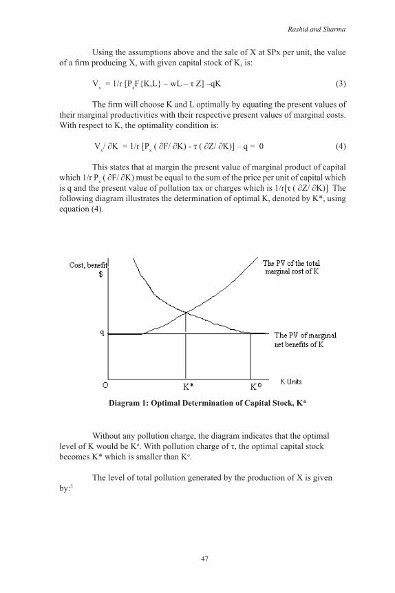
Vx/ ∂K = 1/r [Px ( ∂F/ ∂K) - τ ( ∂Z/ ∂K)] – q = 0 (4)

This states that at margin the present value of marginal product of capital which 1/r Px ( ∂F/ ∂K) must be equal to the sum of the price per unit of capital which is q and the present value of pollution tax or charges which is 1/r[τ ( ∂Z/ ∂K)] The following diagram illustrates the determination of optimal K, denoted by K*, using equation (4).

Diagram 1: Optimal Determination of Capital Stock, K*

Without any pollution charge, the diagram indicates that the optimal level of K would be Ko. With pollution charge of τ, the optimal capital stock becomes K* which is smaller than Ko.

The level of total pollution generated by the production of X is given by:3

Vx = 1/r [PxF{K,L} – wL –! Z] –qK (3)

The firm will choose K and L optimally by equating the present values of their marginal

productivities with their respective present values of marginal costs. With respect to K, the optimality

condition is:

! Vx/! K = 1/r [Px ( ! F/! K) - ! (! Z/! K)] – q = 0 (4)

This states that at margin the present value of marginal product of capital which 1/r Px (! F/! K)

must be equal to the sum of the price per unit of capital which is q and the present value of pollution tax or

charges which is 1/r[! (! Z/! K)] The following diagram illustrates the determination of optimal K,

denoted by K*, using equation (4).

Diagram 1: Optimal determination of capital stock, K*

Without any pollution charge, the diagram indicates that the optimal level of K would be Ko. With

pollution charge of! , the optimal capital stock becomes K* which is smaller than K

o.


Diagram 2: Level of pollution due to capital stock


48

Diagram 2: Level of Pollution due to Capital Stock

Consider now a firm that produces a non-polluting product, call this product as Y. To be consistent with the non-polluting assumptions we have to assume that the production of Y is entirely labour-intensive, viz.,

Y = H(L) (5)

Where H is increasing and concave in L.

The production of Y has to be single-period as in the subsequent period new units of labour will be used for further single-period production. Assume the selling price of Y as $Py per unit, the value of the non-polluting firm is:

VY = 1/(1+r)[PYH(L) – wL} (6)

The optimality condition requires that

1/(1+r) [PY ( ∂H/ ∂L) - w) = 0 (7)

Or PY ( ∂H/ ∂L) = w

3.2 The Case of All Firms in the Economy

It is assumed that total number of polluting firms in the economy is NX, and the total number of non-polluting firms is NY. Within each class, firms are assumed to be identical. As compared to sub-section A above, there are three distinguishing features that emerge. Firstly, there can be an impact on input prices: w, τ and q if there will be a simultaneous expansion (contraction) of outputs X and Y. As a consequence, the level of pollution under this variable input prices situation will be different as compared to the situation of constant input prices. Secondly,

Vx = 1/r [PxF{K,L} – wL –! Z] –qK (3)

The firm will choose K and L optimally by equating the present values of their marginal

productivities with their respective present values of marginal costs. With respect to K, the optimality

condition is:

! Vx/! K = 1/r [Px ( ! F/! K) - ! (! Z/! K)] – q = 0 (4)

This states that at margin the present value of marginal product of capital which 1/r Px (! F/! K)

must be equal to the sum of the price per unit of capital which is q and the present value of pollution tax or

charges which is 1/r[! (! Z/! K)] The following diagram illustrates the determination of optimal K,

denoted by K*, using equation (4).

Diagram 1: Optimal determination of capital stock, K*

Without any pollution charge, the diagram indicates that the optimal level of K would be Ko. With

pollution charge of! , the optimal capital stock becomes K* which is smaller than K

o.


Diagram 2: Level of pollution due to capital stock

Rashid and Sharma

49

the situation of full employment or less than full employment of labour becomes critical for increase (decrease) of the level of pollution. Thirdly, the level of total pollution in the economy at a given point in time is equal to NYZ*, where Z* is the level of pollution that corresponds to optimal K, K* in Diagram 1.

4. The Impact of Interest Rates on Pollution

4.1 The Case of a Single Firm

We all know that interest rate fluctuate. While week-to-week fluctuations are less likely to affect capital expenditures of polluting firms, a durable decrease (increase) in interest rates is expected to raise (lower) investment expenditures.4 Assuming a downward drift in interest rates, causing r to decline, that is d r < 0, firms demand for K rises, resulting an increase VX as in the following equation: 5

Given that d r < 0, the first term on the right hand side is positive. However, despite the fact that ∂F/ ∂K > 0, ∂Z/ ∂K >0, < ∂K/ ∂r < 0 and d r < 0; the second term on the right hand side of (8) is zero due to the optimality conditions given in equation (4). However, for intra-marginal capital projects this term is positive and these intra-marginal projects span between K* and K** in Diagram 3.

Diagram 3: Effect on Capital Stock due to a Decline in Interest Rates

In other words, NPVs of projects between K* and K** are positive, producing the

(! VX/ ! r) d r = ((-1/r2) d r)[PX F(K,L) – wL – ! Z] +

[1/r {PX ! F/! K – ! ! Z/ ! K} – q]( ! K/ ! r) d r (8)

(! VX/ ! r) d r = ((-1/r2) d r)[PX F(K,L) – wL – ! Z] +

[1/r {PX ! F/! K – ! ! Z/ ! K} – q]( ! K/ ! r) d r (8)




50

total NPV equal to the area of EAE´ in the diagram. It is only at point K**, the NPV of the marginal dollar investment is equal to zero. At point E′, the first term of the equation (8) is evaluated as K** level of capital stock.

The upward shift of the PV of MNBK curve indicates the fact that at lower interest rates, the discounted value of the net profits of the firm in the future rises. The new optimality point becomes E´ with corresponding optimal stock of K** which is higher than K*. At K**, there is the higher level of pollution and this rising pollution level explains the upward movement from E to E′ on the curve of the present value of total marginal cost of K. It may be noted that with zero pollution and/or no pollution charge or tax, the optimal level of K would have been K′.

Equation (8) assumes no induced effect of ΔK on labour services, L. But in practice, it is rare that a capital project , in addition to more K, will not involve more L. Incorporating this induced effect, equation (8) will expand involving the following additional term: 1/r[PX ( ∂F/ ∂L) - w] ( ∂L/ ∂K) ( ∂k/ ∂r) d r (9)

However, the first order conditions for optimality implies that for a marginal project, the contribution of this term to the incremental value of the polluting is also equal to zero.

The effect of d r <0 on the value of a non-polluting firm arising solely from the fact that the discounted value of net profit over the period will be higher, although this increase will be substantially smaller than that of a polluting firm. Also, a non-polluting firm does not undertake capital investments because a decline in interest rates does not increase VY due to positive NPV projects.

4.2 The Case of All the Firms

(i) The Scale Effect: In the situation of all the firms in the economy, a decline in interest rates entails two additional channels of influence on the stock of capital and thereby on the total pollution level in the economy. Firstly, a decline in interest rate will induce demand for capital by all polluting firms and the aggregate incremental demand for k will raise its price of q. Secondly6, there will be an induced demand for labour and an upward pressure on the wage rate, w, will depend upon whether the economy is at full employment or it has unemployed labour force. In the full employment economy, the demand for labour by the polluting sector can be met only by a shift of labour from the non-polluting sector to the polluting sector a la Rybczinski theorem. Suppose total L is L in the economy. Then with full employment,

LX + LY = L (10)

Where LX = employment in the polluting sector, and LY = employment in the non-polluting sector

Rashid and Sharma

5151

Which means that

ΔLX = - ΔLY (11)

In this situation the wage rate, w, will tend to rise. Also, the production in the non-polluting sector will shrink. However, if there is sufficient unemployment, then ΔLX can be taken from the pool of unemployed workers. As a consequence, there will not be a demand-driven increase in the wage rate nor will there be any decline in the output of the non-polluting sector. But, to the extent, the pool of unemployment will be sufficient to satisfy the increased demand for labour by the polluting sector, the wage rate will rise-- the increase in w will be lesser relative to the situation of full employment, and similarly, the output of the polluting sector will decline—the decrease will be lesser relative to the situation of full employment.

The marginal project of each polluting firm will face variable input prices. The effect on the value of a polluting firm of a marginal project will now be given by:

( ∂Vx/ ∂r) d r = ((-1/r2) d r) [PX F(K,L) – wL – τ Z] + [1/r {PX ( ∂F/ ∂K) – τ (∂Z/ ∂K)} – ( ∂K/ ∂r) d r + 1/r[PX ∂F/ ∂L – w] ( ∂L/ ∂K) ( ∂K/ ∂r) d r - L/r {( ∂w/ ∂L) ( ∂L/ ∂K) ( ∂K/ ∂r)} d r - K {( ∂q/ ∂K) ( ∂K/ ∂r)} d r (12)

The first three terms in equation (12) are the same as in equations (8) and (9) above while the last two terms reflect the upward pressures on input prices. The term involving ∂w/ ∂L will be zero if there will be sufficient unemployed workers, otherwise it will be positive (with maximum value under full employment) preceding by the minus sign. The optimal conditions for the determination of K and L now become: 1/r [PX ( ∂F/ ∂K) - τ ( ∂Z/ ∂K)] - q – k ( ∂q/ ∂k) = 0 (13)

and

1/r [PX ( ∂F/ ∂L) - w - L ( ∂W/ ∂L)] = 0 (14)

Again, for an intra-marginal project, the NPV will be obtained from the last four terms of the equation (12) which will be positive but for the marginal project, the sum of these term will be zero as reflected by the optimality conditions (13) and (14). Diagrammatically, the determination of the optimal level of K is given as:


52

Diagram 4: Effect on Capital Stock of a Polluting Firm Due to a Decline in Interest Rates in the Economy

Due to increased PV of marginal net benefit, and assuming no effect on the wage rate, w, the PVMNB curves shift to the right to PVMNB′. At the old level of q, the optimal level of K is K′. The rise in q shifts the PVMC´ curve upward to the left reducing optimal K to K″ from K′. If the wage rate would rise as it would be the situation of full employment, the PVMNB curve will shift leftward to PVMNB″. This shift will be somewhat smaller if there will be a pool of unemployed workers. The ultimate optimal level of K is K* which is lesser than under the situation of constant input prices. Equivalently, under the situation of a decline in interest rates, the pollution level will increase at lower pace in an economy where there is full employment. The total increase in pollution will be (G(K*) – G(K^)) x Nx, where Nx is the number of polluting firms in the economy.

(ii) The Composition Effect: Subsection (i) above illustrates the scale effect on pollution, triggered by a decline in interest rates. The composition effect arises from the size of the polluting sector relative to non-polluting sector. This relative size can be measured by contribution of the sector to the gross domestic product, GDP. The GDP in our rudimentary economy is given by:

GDP = NxPxX + NyPyY (15)

Everything else be the same, if the larger is the relative size of the polluting industry, a decline in interest rates will generate a higher level of pollution. The reason for this result is simply this that the polluting sector is assumed to be capital intensive, capital stock is assumed to be source of pollution and a decline in interest rates expand capital investment.

(iii) The Technique Effect: The polluting sector is assumed to use dirtier capital stock. If the technology of this sector were to change to use cleaner or green technology, the pollution level will tend to decline. A decline in interest rates will still stimulate capital investments but the use of green capital stock will be non-

Diagram 4: Effect on Capital Stock of a Polluting Firm Due to

A Decline in Interest Rates in the Economy

Rashid and Sharma

53

polluting.

The theoretical analysis of the model proposes the following testable hypotheses:

Hypothesis 1: Everything else the same, a decline in interest rates will trigger pollution in an economy where capital stock is assumed to be polluting.

Hypothesis 2: Everything else the same, a decline in interest rates will result in a higher level of pollution in an economy which is operating below full employment.

Hypothesis 3: Everything else the same, a decline in interest rates will lead to more pollution in an economy where the pollution charge or tax is zero or relatively lower.

Hypothesis 4: Everything else the same, a decline in interest rates will result in less pollution in an economy where price per unit of capital is more sensitive to the demand for capital.

Hypothesis 5: Everything else the same, a decline in interest rates will trigger more pollution in an economy where the relative size of capital-intensive sector is larger.

Hypothesis 6: Everything else the same, a decline in interest rates will result in less pollution in an economy where cleaner capital stock is also used in production.

An elaborated numerical example will simulate the results of the model next.

5. A Numerical Example

A. The Case of a Single Firm

(i) Polluting Firm Assume: PX = $100 Per unit of X, w = $12.949 per unit of L τ = $100 per unit of pollution, Z q = $1,333 per unit of K, r = 5%

X = F(K,L) = 10K.5 + L.8, and Z = G(K) = K.

Then,


54

VX = 1/.05[100{10K.5 + L.8} – 12.949 x L – 100K] – 1333 x K (16)

The first order conditions for optimality require that

∂ Vx/ ∂K = 1/.05 [100 x .5K-.5 - 100] – 1333 = 0, and ∂Vx/ ∂L = 1/.05 [100 x .8L-.2 - 12.949] = 0 (17) The system of equations in (17) solve for K =9 units and L = 9,000 units. Thus the optimal levels of K and L for the polluting firm is (K*, L*) = (9,000). The corresponding Vx and the level of a polluting firm is:

VX* = 1/.05 [100 {10 x 9.5 + 9000.8} – 12.949 x 9000 – 100 x 9] –

1333 x 9 = $612,743, and

Z* = 9 units of pollution

(ii) A Non-polluting Firm

Assume, PY = $30 and Y = F (L) = 2L.8. Then VY = 1/1.05[30 x 2L.8 – 12.949 x L] (18)

The optimal level of L is given by

∂VY/ ∂L = 1/1.05[60 x 0.8L-.2 – 12.949] (19)

This gives L* = 669.9 units.

Thus VY = .9524 [30 x 2(669.9) .8 – 12.949 x 669.9 = $2,156.33

B. The Effect of Interest Rate on Pollution

(i) The Case of Unemployed Workforce

In this situation, input prices are assumed to remain constant. Assume d r = -.01, that is the level of the discounted rate, r, becomes r = .04.

Now,

Rashid and Sharma

55

VX = 1/.04 [100 {10 x 10K.5 + L.8} – 12.949 x L – 100 x K] – 1333 K (20)Again, from the first order condition, similar to the system of equations

in (17), except r is now 4% instead of 5%, the optimal levels of K and L become: K* = 10.635 and L* = 9000.54 units. The incremental demand for K is 1.635 units. This is the additional investment the firm undertakes. As a consequence of above changes, we have

VX = 1/.04 [100 {100 (10.635).5 + 9000.54}.8 – 12.949 x 9000.54100 x 10.635] – 1333 x 10.635–

This gives VX = $716,184. The new level of pollution is 10.635 units.

As compared to the situation of r = 5%, the firm’s value rises by $156,441.

As far as the non-polluting firm is concerned, its optimal L remains at 669.9 units, but its market value rises to $2,177.02 due to a decline in interest rates.

(ii) The Case of Full Employment

In this situation, input prices will tend to rise. We assume that

d w/d r = -30, and d q/d r = -2000

Given these assumptions, and noting that d r = -0.1, we have d w = -30 x -01 = $0.3, and d q = (-2000) (-0.01) = $20. Thus, the new levels of w and q become:

w´ = w +d w = 12.949 + 0.3 = $13.249 q´ = q + d q = 1,333 + 20 = $1,353

With all the previous assumptions and the new levels of w and q, the market value of the polluting firm becomes: V´´X = 1/.04 [100 {10K.5 + L.8} – 13.249 x L – 100K] – 1353 K

The first order conditions for optimality provide the optimal levels of K and L as K**, L** = (10.525, 8,026.65). It may be noted that the investment level shrinks somewhat and the use of labour declines. These results are consistent with the theory presented earlier in the paper.

At the new optimal levels of K, L, VX becomes $705,240. It is still higher relative to the situation of r = 5%, but the increase in VX is somewhat less, as


56

expected. The level of pollution generated by the firm is now 10.525 units.

At the higher wage rate, the use of labour by a non-polluting firm declines to 624.15 units—a decline of 45.74 units. And despite lower interest rates, the market value of this firm declines to $1,987.7—a $168.62 reduction.

6. Summary and Conclusions

In this paper, we have argued that durable changes in interest rates affect the level of pollution in an economy. This effect is shown to arise from a realistic assumption that capital intensive production generates pollution, and declines in interest rates stimulate capital investment. We have proposed a theoretical model to study this effect. The model consists of two sectors: capital intensive or a polluting sector and labour intensive or a non-polluting sector. Some interesting results of the paper are: (i) A decline in interest rates will result in a lower increase in the level of pollution in an economy that is operating at or near full employment relative to an economy that is operating with unemployed labour force. (ii) A decline in interest rates will trigger less increase in pollution in an economy where input prices are more sensitive to input demands than in an economy where they are less sensitive. The model of the paper has suggested a series of testable hypotheses about the effect of interest rates on pollution. The next steps in our research are to do empirical tests of the suggested hypotheses of the model and, secondly, to extend the model to an open economy so that the cross-country variations in interest rates, differences in pollution charges, regulation, tax structures, industrial structures and input prices can be fully incorporated into the analysis.

Endnotes

1As noted in the previous section, pollution may be related to air, water or soil and within each category, there are multitudes of pollutants. It is most likely that some pollutants are more responsive to capital stock than others. However, we abstract from this detail here, and assume as if all pollutants are homogeneous.

2Research aimed at estimating the shadow price or social cost of per unit of pollution provide diverse estimates. Tol (2005) presents a survey of the literature on the estimates of the marginal damage cost of per ton carbon dioxide omission and finds a range of minus $4 to $,1666. Tol and Lyons (2008) report the current price of the European Trading System for carbon dioxide emission permits which ranged from Euro 33 to Euro .01 over the January 2006 and February 2008 period. In our static model, we assume the social cost per unit as simply $τ .

3For ease of calculations in the numerical section of the paper, we assume function G in equation (2) as a simple linear function.

4Interest rates in the developed countries generally rose from late 1960s to 1981 and subsequently, generally fell until 1992. Interest rates again rose, but modestly, from 1992 to 2002, and since 2002 interest rates have been basically stable.

5An increase in r, that is d r > 0 will have opposite effects to those which arise with respect to d r < 0.

6We are assuming that τ is a pollution charge or tax imposed by the government. If τ were to be interpreted as the price of marketable pollution permits, τ will also be affected as an increase in K will cause more firms to demand for pollution. Here we assume τ to be fixed.

Rashid and Sharma

57

References:

Boyce, J. 1994. Inequality as a cause of environmental degradation. Ecological Economics, 11:169-78.

Brown, Katrina and Esteve Corbera. 2003. Exploring equity and sustainable development in the new carbon economy. Climate Policy, 3(S1) :41-56.

Bullard, R. 2000. Dumping in Dixie: Race, Class and Environmental Quality, 3rd. ed. Boulder, Co: Westview Press.

Copeland, Brian R. and M. Scott Taylor. 2004. Trade, growth and the environment. Journal of Economic Literature, 42:7-71.

Davidson, P. and D. Anderson. 2000. Demographics of dumping II: A national environmental equity survey and the distribution of hazardous materials handlers. Demography, 37(4):461-66.

Ederington, Josh. 2007. NAFTA and the pollution haven hypothesis. The Policy Studies Journal, 35(2):239-244.

Fisher, L. F. 1971. Dimensions of environmental crisis. Zygon, 5(4):274-283.

Frankel, Jeffrey A. and Andrew K. Rose. 2005. Is trade good or bad for the environment? Sorting out the causality. The Review of Economics and Statistics, 87(1):85-91.

Gamper-Rabindran, S. 2006. NAFTA and the environment: What can the data tell us? Economic Development and Cultural Change, 54(3):606-633.

Grossman, G. M. and Anne B. Krueger. 1995. Economic growth and the environment. Quarterly Journal of Economics, 110:353-377.

Harbaugh, William T., Arik Levinson, and David Molloy Wilson. 2002. Reexamining the empirical evidence for an environmental Kuznets curve. The Review of Economics and Statistics, 84(3):541-551.

Harrison, Kathryn and Lisa McIntos Sundstrom. 2007. The comparative politics of climate change. Global Environmental Politics, 7(4):1-18.

Huang, W. M, Grace W. M. Lee and C. C. Wu. 2008. GHG emissions, GDP growth and the Kyoto protocol: a revisit of environmental Kuznets curve hypothesis. Energy Policy, 36:239-247.


58

King, P.N. and H. Mori. 2007. The development of environmental policy. International Review for Environmental Strategies, 7(1):7-16.

Pearce, David. 2003. The social cost of carbon and its policy implications. Oxford Review of Economic Policy, 19(3) : 362-384.

Rauch, James E. 2005. Getting the properties right to secure property rights: Dixit’s Lawlessness and Economics. Journal of Economic Literature, XLIII (2) : 480-487.

Ringquist, E. 1998. A question of justice: Equity in environmental litigation, 1974-1991. Journal of Politics, 60(4):1148-65.

Roberts, J.T., P. E. Grimes and J.L. Manale. 2003. Social roots of global environmental change: A world-systems analysis of carbon dioxide emissions. Journal of World-Systems Research, 9(2): 277-315.

Rosser, J. Barkely and Marina V. Rosser. 2006. Institutional evolution of environmental management under global economic growth. Journal of Economic Issues, XL(2): 421-429.

Smith, Fred. 1995. Markets and the environment: A critical reappraisal. Contemporary Economic Policy, 13: 62-73.

Solakoglu, E. G. 2007. The effect of property rights on the relationship between economic growth and pollution for transition economies. Eastern European Economics, 45(1) : 77-94.

Stern, D. I. 2004. The rise and fall of the environmental Kuznets curve. World Development, 32(8), 1419-1439.

Taiyab, Nadaa. 2006. Exploring the market for voluntary carbon offsets. International Institute for Environment and Development, London.

Tiemstra, J.P. 2003. Environmental policy for business and government. Business and Society Review, 108 (1): 61-69.

Tol, Richard S. J. 2005. The marginal damage costs of carbon dioxide emissions: An assessment of the uncertainties. Energy Policy, 33 : 2064-2074.

Tol, Rrichard S. J. and Sean Lyons. 2008. Incroporating GHG emission costs in the economic appraisal of projects supported by state development agencies. Working Paper No. 247, Economic and Social Research Institute, Dublin, Ireland.

Torras, Mariano. 2005. Income and power inequality as determinants of environmental and health outcomes: some findngs. Social Science

Rashid and Sharma

59

Quarterly, 86: 1354-1376.

World Bank.1992. World Development Report 1992. New York: Oxford University Press.

Interest Rates and Environmental Pollution

Documents

Transcript of Interest Rates and Environmental Pollution