Interest Rates and Credit Risk∗

Carlos González-Aguado

Bluecap M. C.

Javier SuarezCEMFI and CEPR

February 2012

Abstract

This paper explores the effects of shifts in interest rates on corporate leverageand default. We develop a dynamic model in which the relationship between firmsand their outside financiers is affected by a moral hazard problem and entrepreneurs’initial wealth is scarce. The link between leverage and default risk comes from thelower incentives of overindebted entrepreneurs to guarantee firm survival. The need tofinance new investment with outside funding pushes firms’ leverage ratio above somestate-contingent target towards which they gradually adjust through earnings retention.The dynamic response of leverage and default to interest rate rises and cuts is bothasymmetric and heterogeneously distributed across firms. Both rises and cuts increasethe aggregate default rate in the short-run. However, a higher interest rate reducesfirms’ target leverage and hence produces lower default rates in the longer run. Thishelps rationalize some evidence regarding the risk-taking channel of monetary policy.

Keywords: interest rates, short-term debt, search for yield, credit risk, firm dynamics.

JEL Classification: G32, G33, E52.

∗We would like to thank Oscar Arce, Arturo Bris, Andrea Caggese, Xavier Ragot,Rafael Repullo, Enrique Sentana, David Webb and seminar participants at the 2009European Economic Association Meeting, the 2010 World Congress of the Economet-ric Society, Banco de España, Bank of Japan, CEMFI, CNMV, European CentralBank, Instituto de Empresa, Norges Bank, Swiss National Bank, Universidad CarlosIII, Universidad de Navarra, the XVIII Foro de Finanzas, and the JMCB conference“Macroeconomics and Financial Intermediation: Directions Since the Crisis” for helpfulcomments and suggestions. Contact e-mails: cgonzalez@bluecap.es, suarez@cemfi.es.

1

1 Introduction

The experience surrounding the Great Recession of 2008-2009 has extended the idea that

long periods of low (real) interest rates may have a cost in terms of financial stability.

Many observers believe that keeping interest rates “too low for too long”–as it happened

during the Greenspan era–contributed to aggregate risk-taking in the years leading to the

crisis. Concepts such as search for yield (Rajan, 2005) and risk taking channel of monetary

policy (Borio and Zhu, 2008) have been coined to refer to the phenomenon whereby financial

institutions, in particular, might have responded to low real interest rates by accepting higher

risk exposures. One manifestation of such exposures would be the unprecedented pre-crisis

leverage of the private non-financial sector, which surely contributed to the high default rates

observed after things turned wrong.

Formal empirical evidence on these issues is relatively recent and suggests that the under-

lying phenomena are quite complex. In fact one first complexity refers to properly identifying

causal relationships, since movements in real interest rates, even when driven by discretionary

monetary policy decisions, constitute endogenous reactions to prior or parallel developments

in the real and financial sectors. Ioannidou et al. (2009), Jimenez et al. (2011), and Mad-

daloni and Peydró (2011) provide evidence that reductions in interest rates are followed by a

deterioration of lending standards, an increase in lending volumes, and, with some additional

lag, by rises in default rates.1 From here it would be tempting to conclude that lowering

interest rates increases credit risk across the board but several arguments call for a more

cautious analysis. Specifically, some evidence supports the view that high short-term inter-

est rates increase credit risk, at least in the short run and certainly for the most indebted

borrowers.2 Additionally, as our analysis below confirms, financial frictions may cause the

effects of interest rate rises and interest rate cuts not to be symmetric, especially in the short

run, when over-indebted borrowers may not be able to immediately adjust to lower leverage

targets.

1See also Altunbas et al. (2010).2Jacobson et al. (2011) find that short-term interest rates have a significant positive impact on default

rates among Swedish firms, and that the effect is stronger in sectors characterized by high leverage. In aclinical study, Landier et al. (2011) argue that interest rate rises started in 2004 could have pushed a majorUS subprime morgage originator into making riskier loans.

2

The objective of this paper is to develop an infinite horizon model of the effects of interest

rates shifts on corporate leverage and corporate default. Theoretical work on this topic is

scarce, possibly due to the difficulty of putting together corporate finance frictions and the

root causes of interest rate shifts (e.g. monetary policy). Several papers have looked at

the issue in essentially static, non-monetary models that represent monetary policy as an

exogenous shift in investors’ opportunity cost of funds (or in the real risk-free interest rate).

Examples of this approach go back to Stiglitz and Weiss (1981) and include Mankiw (1986),

Williamson (1987), Holmstrom and Tirole (1997), Repullo and Suarez (2000), and Bolton

and Freixas (2006).3

In macroeconomics, the topic has been mainly examined by the literature on the credit

channel of monetary policy. Carlstrom and Fuerst (1997) and Bernanke, Gertler, and

Gilchrist (1999) focus on the dynamics of an external financing premium which reflects

the deadweight costs of a static costly-state-verification contract–where verification is the

model counterpart of default. However, like in the banking papers cited above, firms’ financ-

ing problems are formulated as essentially static, using an overlapping generations structure.

In the credit to the entrepreneurs in Kiyotaki and Moore (1997) and to the banks in Gertler

and Kiyotaki (2010), like in many other papers, default is an out-of-equilibrium phenomenon.

Our paper fits in the literature that looks at genuinely dynamic corporate finance prob-

lems in an (industry or general) equilibrium setup. In this literature, some papers focus on

optimal dynamic financing decisions under given contractual forms (Cooley and Quadrini,

2001, Hennessy andWhited, 2005, Cooley and Quadrini, 2006, Hackbarth et al., 2006, Morel-

lec at al., 2008), while others look at optimal dynamic contracts (Clementi and Hopenhayn,

2006, DeMarzo and Fishman, 2007). Among these papers, only Cooley and Quadrini (2006)

consider the effects of shocks to a bank lending rate controlled by the monetary authority in

a model where firms access external finance through a sequence of short-term debt contracts.

They obtain responses of leverage to rises in lending rates similar to ours (and with similar

heterogeneity across firms) but they do not discuss asymmetric responses to interest rate

rises and cuts and in their framework default never occurs in equilibrium.

3In all these papers, “monetary policy” has an impact on the amount of credit but not necessarily oncredit risk. For example, in Holmstrom and Tirole (1997), the binary-action formulation of the underlyingmoral hazard problem makes equilibrium default risk equal to one of the parameters of the model.

3

We contribute to the first strand of this literature by focusing on the effects of interest rate

shocks on credit risk. Our model is characterized by three key features. First, firms obtain

outside financing using short-term debt contracts.4 Second, their relationship with outside

financiers is affected by a moral hazard problem like in Holmstrom and Tirole (1997) and

Repullo and Suarez (2000), although the problem in our case involves genuinely dynamic

trade-offs since entrepreneurs make a continuous unobservable decision on private benefit

taking in every period that has a continuous (negative) impact on the probability that the

firm survives into the next period. Third, the opportunity cost of funds of the outside

financiers (the short-term risk free rate) follows a Markov chain. So interest rate shocks are

an integral part of the environment and, when firms make their financing decisions, they

know that future rates may change.

The model also features endogenous entry and exit. Like in other papers in the literature,

we assume that entrepreneurs always discount the future at a higher rate than outside

financiers, providing a prima facie case for the outside financing of their firms even in the

long run.5 Entering entrepreneurs start up penniless (and hence need debt to undertake their

initial investments) but, once their firms are active, they can use earnings to reduce their

firms’ leverage. Alternatively, they can pay dividends (which are immediately consumed) to

themselves. Entrepreneurs running non-surviving firms leave the economy forever. Finally,

the (costly) entry of novel entrepreneurs prevents the measure of active firms from going to

zero.6

The model delivers leverage ratios and default probabilities that are maximum imme-

diately after undertaking the new investment and then, ceteris paribus, decrease as firms

gradually move towards their target leverage ratios through earnings retention. Firms with

4The assumption regarding the sole use of short-term debt can be relaxed by considering situations inwhich (in every period) the firm can buy a (variable) amount of insurance against a shift in the short-termrate in the subsequent period. Alternatively, one can extend the analysis to the case in which the firmcan issue long-term debt (e.g., to facilitate tractability, some amount of consols) at the start-up date. In apreliminary analysis of these extensions we found no qualitative changes in our results.

5Entrepreneurs’ larger discounting can be justified as a result of unmodelled tax distortions that favoroutside debt financing, or as a reduced-form for the discount for undiversifiable idiosyncratic risk that wouldemerge if entrepreneurs were risk averse.

6As a convenient way of capturing congestion (or aggregate decreasing returns to scale) in finding aprofitable investment opportunity, we assume that the costs of entry of candidate entrants is increasing inthe number of already existing firms.

4

excess leverage have lower continuation value and, thus, greater incentives to extract private

benefits and put their continuation at risk. Moreover, under the equilibrium levels of lever-

age that the model generates, non-surviving firms always default on their debts, producing

an intuitive correlation between leverage and credit risk.7

We find that, due to the underlying financial frictions, (i) interest rate cuts and interest

rate rises have asymmetric effects on leverage and default, (ii) the response to interest rate

shifts is heterogeneous across firms, and (iii) interest rate shifts have different implications

for leverage and default in the short run than in the longer run. The asymmetries are due

to the fact that, due to the need to rely on retained earnings for leverage reductions, it is

easier to adjust leverage up (following interest rate cuts) than down (following rises). In fact,

for the firms that are above target leverage, a rise in interest rates may imply a temporary

increase in leverage and credit risk (due to the extra cost of their outstanding debt).8

The heterogeneity in the response of firms to interest rate shifts is relevant because the

presence of endogenous exit and entry makes not all firms equally levered when a shift occurs.

Opposite to firms already at their target leverage, rises in interest rates produces a temporary

increase in leverage and default risk among over-indebted firms that are trying to approach

their target. In contrast, the effects of interest rate cuts are of the same sign for firms at

or above their target leverage, although quantitatively more pronounced for the latter since

lower rates allow them to speed up the convergence to the target.

The propagation of the effects of interest rate shifts over time is mainly explained by the

fact that interest rate shifts (which are quiet persistent in the calibration) change firms’ target

leverage. The shifts typically find many firms in their old target (and the rest converging to

it). The strong initial effect dampens away as the adjustment to the new target is completed.

In addition, the exit of the firms that fail and the entry of replacing new firms that start

up with higher leverage produces a non-trivial and evolving distribution of firms over different

leverage levels (and levels of credit risk). We use the law of motion of this distribution to

7See Molina (2005) for a recent restatement of the importance of leverage as a determinant of defaultprobabilities.

8The empirical literature on the effects of monetary policy shocks on real output have also found asym-metries (e.g. Cover, 1992, or Weise, 1999), typically attributed to nominal rigidities. To the best of ourknowledge, the potential asymmetric effects of interest rate shocks on corporate leverage and default havenot been directly analyzed at either an individual firm level or the aggregate level.

5

analyze the implications of the model for aggregate leverage and aggregate default. Under

our parameterization of the model (partly chosen so as to match moments prevailing among

US firms), we obtain the somewhat surprising result that both interest rate rises and interest

rate cuts produce short run increases in the default rate. This means that the transitional

leverage-increasing effect observed among highly levered firms drives up the aggregate default

rate immediately after interest rate rises, while the impact of interest rate cuts is explained

by the increase in target leverage across all firms. In the longer run, interest rate rises reduce

target leverage and, hence, end up decreasing aggregate leverage and default, while interest

rate cuts have the opposite effects.

All in all, the paper provides a possible rationalization of some of the empirical find-

ings that the literature mentioned in the opening paragraphs tends to interpret as due to

“search for yield” incentives among financial institutions and evidence of a risk taking chan-

nel of monetary policy. Interestingly, our rationalization is based on the dynamic extension

of a pretty canonical moral hazard model of the relationship between firms and their out-

side financiers (see Tirole, 2005) and does not rely on irrational agents (e.g. Shleifer and

Vishny, 2010) or on ad hoc accounting rules, risk-management techniques, and managerial

compensation practices (e.g. Adrian and Shin, 2010).

To facilitate tractability (and transparency about the mechanism behind our results), we

make various assumption (fixed firm size, ex ante homogeneity, lack of initial entrepreneurial

wealth) that leave aside many potentially important phenomena regarding firms’ life cycle

(growth, learning about firms’ types, dynamic selection based on the survival of the fittest,

etc.). Likewise, the macroeconomic environment is solely described by the exogenous process

driving interest rate shifts and the analysis looks at the corporate sector in isolation, with-

out considering feedback effects. Strictly speaking, our analysis provides the ceteris paribus

implications of interest rate shifts on a highly stylized representation of the corporate sector.

Yet these implications suggest a candidate explanation for some apparently contradictory

results about the link between monetary policy and credit risk found in the empirical liter-

ature. Asymmetries and sources of heterogeneity in the response to interest rate shifts like

the ones identified in the model might explain the ambiguous or mixed signs of the aggregate

effects found using linear regression models. Our analysis points to the explicit consideration

6

of these issues (and the complexity of aggregation in their presence) as a fruitful strategy for

future research.

The paper is organized as follows. Section 2 describes the model. Section 3 studies

the case without aggregate uncertainty regarding interest rates, for which we can obtain

analytical results. Section 4 extends the characterization of equilibrium to the case with

aggregate uncertainty regarding interest rates, presents the parameterization used in the

numerical analysis, and discusses the results regarding the effects of interest rate shifts.

Section 5 discusses the consistency of our results with the literature on firms’ life cycle

and other corporate finance evidence, and elaborates on their macroprudential implications.

Section 6 concludes.

2 The model

We consider an infinite-horizon discrete-time economy in which dates are indexed by t =

0, 1, ... and there are two classes of risk-neutral agents, entrepreneurs and financiers.

2.1 Model ingredients

There many competitive financiers with deep pockets and the opportunity of investing their

funds in a reference short-term risk-free asset that yields a rate of return rt during the period

between dates t and t+1. This rate follows a Markov chain with two possible values rL and

rH , with rL ≤ rH and a time-invariant transition probability matrix Π = {πij}j=L,Hi=L,H , where

πij = Pr[rt+1 = rj | rt = ri]. rt realizes at the beginning of each period.

A new cohort of entrepreneurs, made up of a continuum of individuals, is born at each date

t. Entrepreneurs are potentially infinitely-lived and their time preferences are characterized

by a constant per-period discount factor β < 1/(1+rH) so that entrepreneurs have incentives

to rely on outside funding even if they are able to self-finance their firms.

Entrepreneurs are born penniless and with a once-in-a-lifetime investment opportunity.

By incurring a non-pecuniary idiosyncratic entry cost θ at date t, each novel entrepreneur

can find a project whose development gives rise to a new firm. The distribution of θ across

novel entrepreneurs is described by a cumulative distribution (or measure) function F (θ, nt)

which depends negatively on the measure nt of firms operating in the economy at date t. The

7

fact that the costs of finding a project are increasing (in the sense of first order stochastic

dominance) in the measure of active firms, provides an equilibrating mechanism for the entry

of new firms (and for the determination of nt).

Each project requires an unpostponable initial investment normalized to one and the

continued management by the founding entrepreneur. Each project operative at date t has a

probability pt of remaining productive at date t+1. A productive project generates a positive

cash flow y per period. With probability 1 − pt the project fails, in which case it yields a

liquidation cash flow L (out of the residual value of the initial investment) and disappears

forever. The discretionary liquidation of the project at any date also yields L.

Importantly, the continuation probability pt is determined by an unobservable decision

of the entrepreneur which also affects the flow of private benefits u(pt) that he extracts from

his project in between dates t and t+ 1. For notational simplicity, we assume those private

benefits to accrue at t + 1 independently of whether the project fails. We assume u(·) tobe decreasing and concave, and with enough curvature to guarantee interior solutions for

pt.9 Thus, entrepreneurs can appropriate a larger (but marginally decreasing) flow of private

benefits by lowering their probability of continuation. This creates a moral hazard problem

in the relationship between entrepreneurs and financiers.

Insofar as a project remains productive, the entrepreneur can raise outside financing

issuing short-term debt. Such debt is described as a pair (bt, Rt+1) specifying the amount

lent by the financiers, bt, and a repayment obligation from the entrepreneur to the financiers

after one period, Rt+1. At t+1, if the firm fails or is unable to obtain the funds necessary to

pay Rt+1, then the project is liquidated and financiers are paid the whole liquidation value

L.10 Otherwise, the firm decides on its financing for the next period subject to its uses and

sources of funds equality:

ct +Rt = y + bt,

where ct denotes the entrepreneur’s dividend. We impose ct ≥ 0 to reflect that the entrepre-9A sufficient condition to guarantee this would be having u0(0) = 0 and u0(1) = −∞. In the numerical

part of the analysis, we use a specification of u(·) which does not satisfy these properties but we check thatthe resulting solutions are always interior.10The assumption that financiers are paid the whole L (rather than min{Rt+1, L}) greatly simplifies the

notation but is inconsequential since, under any of the two modeling alternatives, the optimal Rt+1 is alwayslarger than L.

8

neur is assumed to hold no outside wealth with which to recapitalize the firm.

2.2 Discussion of the ingredients

We have described rt as the return of a short-term risk-free investment alternative available

to financiers, but other interpretations are possible. It may capture a deeper time-preference

parameter, an international risk-free rate relevant for a “small open economy,” or a convo-

lution of exogenous factors that determine financiers’ required expected rate of return.11 A

n-state Markov process is a simple way to capture uncertainty regarding the evolution of

this variable. The n=2 case facilitates computations and is useful to fix intuitions.

The assumption that entrepreneurs have larger discount rates than their financiers is

common in the literature (e.g. Cooley and Quadrini, 2001). It provides a prima facie case

for entrepreneurs’ to keep relying on external financing. If outside financing takes the form

of debt and inside financing takes the form of equity (as it is typically the case in practice

and several corporate finance theories have justified), one might interpret this assumption

as a result of net tax advantages of debt financing.12 Alternatively, the assumption may

capture the fact that the return entrepreneurs require on the wealth invested in their own

projects is larger than the returns financiers require on presumably better diversified and

more liquid investment portfolios.

The focus on short-term debt is also standard in the literature (e.g. Kiyotaki and Moore,

1997, and Cooley and Quadrini, 2001) and is adopted mainly for tractability: it makes the

state variable that describes the firm’s capital structure unidimensional. Allowing for debts

with arbitrary maturities, possibly issued at different dates and under different conditions

would unbearably multiply the dimensions of the state space. We have explored the model

under alternative financial structures which can still be described in a compact manner (e.g.

those in which, at the start-up date, short-term debt is combined with arbitrary amounts of

11This interpretation might include thinking about rt as a reduced-form for the risk-adjusted required rateof return that risk-averse but well-diversified financiers demand on the securities issued by the entrepreneurs.Closing the model along these lines would require referring explicitly to the systematic and non-systematiccomponents of the risk attached to those securities, and any other determinant of investors’ required riskpremia. Intuitively, rL and rH might correspond to situations in which systematic risk is perceived to below and high, respectively, perhaps due to the intensity of the correlation between project failures.12For a calibration of the tax advantage of debt, see Hennessy and Whited (2005).

9

consols) and the results are qualitatively and quantitatively very similar.13

Finally, to explain imposing ct ≥ 0, notice that entrepreneurs are assumed to be bornpenniless and their outside wealth will thus remain zero if they immediately consume the

dividends received from the firm, which is likely to be optimal given that entrepreneurs are

assumed to be more impatient than their outside financiers at all dates. In fact, one might

suspect that self-insuring against the risk of a shift in the cost of outside funding might be

a reason for active entrepreneurs to hold some precautionary savings outside their firms.

However, in our model, if the best return an entrepreneur could obtain on funds invested

outside the firm for a period is rt, nothing would make those precautionary savings superior

to precautionary savings held within the firm, which in the context of our model are fully

equivalent to just reducing the firm’s leverage during such period.14

3 The case without aggregate uncertainty

This section focuses on firms’ dynamic financing decisions in the economy in which financiers’

opportunity cost of funds, the risk free rate rt, remains constant, i.e. rL = rH = r. In the ab-

sence of this source of aggregate uncertainty, the solution to the firms’ dynamic optimization

problem and its implications for firm entry can be analytically characterized. The analytical

results will help understand the logic of the numerical results obtained for the economy with

random fluctuations in rt.

3.1 Firms’ dynamic financing problem

Without uncertainty about the risk-free rate, the only state variable relevant for the optimal

dynamic financing problem of a firm that remains productive at a given date is the repayment

obligation R derived from the debt issued in the prior debt. Such a firm will have a cash flow

y resulting from its prior period of operation and will have to decide on the debt issued in the

13By considering a limited set of standard financing alternatives, our analysis falls within the classicalcapital structure tradition.14In our model, reducing firm leverage during one period is weakly preferred to keeping an equivalent

amount of precautionary savings outside the firm because, if anything, the first alternative has the advantageof reducing the agency conflicts between the entrepreneur and his financiers (e.g. if limited liability provisionsconstrain his capacity to commit to use the precautionary savings to actually recapitalize the firm in somestates of the world).

10

current date (b, R0), where, to skip time subscripts, we use the convention of identifying the

state variable for the next date as R0. The dividend resulting from the refinancing decision

will be c = y + b − R ≥ 0. To take into account the moral hazard problem derived from

the unobservability of the entrepreneur’s choice of p, we extend the description of the debt

contract to the triple (p, b,R0) and establish the connection between p and the pair (b,R0)

through an incentive compatibility condition.

Assuming that the firm that remains productive is always able to find financing for one

more period, its optimal dynamic financing problem can be stated in the following recursive

terms:15

v(R) = maxp,b,R0

(y + b−R) + β[u(p) + pv(R0)] (1)

subject to

p = arg maxx∈[0,1]

u(x) + xv(R0), (2)

pR0 + (1− p)L = b(1 + r), and (3)

y + b−R ≥ 0, (4)

where v(·) is the entrepreneur’s value function. The right hand side in (1) reflects that theentrepreneur maximizes his dividend in the decision date plus the discounted value of the

private benefits u(p) received in the next date plus the discounted expected continuation

value after one period –continuation value to the entrepreneur is v(R0) if the firm remains

productive and zero otherwise.16

Equation (2) is the entrepreneur’s incentive compatibility condition which entails a trade-

off between the utility derived from private benefits u(p) (decreasing in p) and the expected

continuation value pv(R0) (increasing in p). Since we have assumed that the curvature of

u(p) is enough to guarantee interior solutions for p, the first order condition

u0(p) + v(R0) = 0 (5)

can be conveniently used to replace (2).

15We will not formalize the uninteresting case of non-failing firms which, following an explosive debtaccumulation path, become unable to refinance their debt after a number of periods. Under resonableparameterizations those paths are incompatible with obtaining funding for the initial investment.16Recall the comment made in Footnote 10.

11

Equation (3) is the participation constraint of the financiers–it says that the effective

repayments received after one period (R0 in case of success and L in case of failure) must

imply an expected return r on the extended funding b.17 The third and last constraint (4)

imposes the non-negativity of the entrepreneur’s dividend.

In order to reduce the maximization problem in the RHS of (1)–the stage problem–to

one with a single decision variable and a single constraint, we establish the following intuitive

result. All proofs are in the Appendix.

Lemma 1 The value function v(R) is strictly decreasing for all leverage levels R for which

refinancing is feasible.

With v(R0) < 0 and u0(p) < 0, (5) implicitly defines a function p = P (R0), with P 0(R0) <

0. Using it to substitute for p and solving for b in (3) yields:

b = B(R0) ≡ 1

1 + r[L+ P (R0)(R0 − L)]. (6)

This function has a slope

B0(R0) =1

1 + r[P (R0) + P 0(R0)(R0 − L)] <

1

1 + r(7)

which, assuming P (L) > 0, is definitely positive for R0 close to L, but may become negative

for some larger values of R0. Hence, as in other corporate finance problems, the relationship

between debt value b and the promised repayment R0 may be non-monotonic, although of

course only the upward sloping section(s) of B(R0) would be relevant when solving (1). To

avoid complications related to discontinuities that may emerge if B(R0) has several local

maxima, we adopt the following assumption:

Assumption 1 B(R0) is single-peaked, with a maximum at some R.

This assumption is always satisfied under the parameterizations explored in the numerical

part of the paper.18

17We have written it directly as an equality since, rather than leaving a surplus to the financiers, entre-preneurs would trivially prefer to pay such surplus as a contemporaneous dividend to themselves.18Expressing the assumption in terms of primitives is difficult, since P (R0) involves the value function

v(R0) which can only be found by solving the optimization problem.

12

Using the function B(R0) (which embeds (2) and (3)), the stage problem in (1) can be

compactly expressed as:

maxR0

y +B(R0)−R+ β[u(P (R0)) + P (R0)v(R0)] (8)

s.t.: y +B(R0)−R ≥ 0, (9)

where the only decision variable is R0 and the only remaining constraint is a rewritten version

of (4). Our first proposition establishes the key properties of the solution to this problem.

Proposition 1 The solution to the equation B0(R∗)+βP (R∗)v0(R∗) = 0, if it exists, defines

a unique target leverage level R∗ ≤ R such that:

1. For R ≤ [0, R], where R ≡ y + B(R∗), the non-failing firm issues new debt R0 = R∗,

current debtholders get fully paid back, and the entrepreneur’s dividend is y+B(R∗)−R.

2. For R ∈ (R, y + B(R)], the firm issues new debt R0 = B−1(R − y) ∈ (R∗, R], currentdebtholders get fully paid back, and the dividend is zero.

3. For R > y +B(R), the firm cannot be refinanced and is liquidated.

3.2 Implied dynamics

The analysis of the dynamics of the short-term debt of a non-failing firm can be described

with reference to a phase diagram whose elements emanate directly from Proposition 1.

Figure 1 describes a situation in which there is a unique stable steady state with some

leverage level R = R∗ that non-failing firms reach in finite time.

The diagrammaps a non-failing firm’s current repayment obligationR onto its repayment

obligation in the following date R0. The thicker curve represents the mapping of R into R0

according to the firm’s optimal refinancing decisions. By Proposition 1, such curve is piece-

wise defined by the horizontal line R0 = R∗ which corresponds to the target leverage ratio

and the upward sloping curve implicitly defined by the boundary of the refinancing constraint

(9). This boundary can be described as R0 = B−1(R − y), which is directly connected to

(the inverse of) the upward-slopping section of the single-peaked B(R0) schedule. This curve

has a slope strictly larger than one (since B0(R0) < 1) and is defined for R ∈ [y, y + B(R)]

13

(since for R < y, any R0 > 0 satisfies (9)). Satisfying (9) requires choosing R0 ≤ B−1(R−y).

Hence, given the relative position of this curve and the horizontal line R0 = R∗, it is obvious

that reaching the target R∗ is feasible if and only current repayment obligations are R ≤R ≡ y +B(R∗). Thus the phase diagram describing the dynamics of R is given by the thick

inverse-L shaped curve in Figure 1.

R* R R y+B(R)^ = R

R’

L

R*

R=

45o

1+y_

y+L/(1+r)

R0

y

Figure 1. Phase diagram with a stable steady stateThis figure plots the repayment obligation R0 that results from the optimalrefinancing decision of a non-failing firm whose current repayment obligation isR. The arrows indicate the dynamics of the firm’s repayment obligation alonga non-failing path that converges in five periods to the target leverage level.

In Figure 1 the phase diagram crosses the 45-degree line twice, once on the horizontal

section, at R = R∗, and another time on the vertical section, at a point denoted R = bR. Thisis just one of the three possible situations that one may have. Alternatively, the piece-wise

curve may fully lay to the left of the 45-degree line, but in this case, refinancing dynamics is

explosive. As yet another alternative, the curve may intersect the 45-degree line only once,

on its horizontal section, which will be the case if y + B(R) < R. In this case refinancing

dynamics is qualitatively the same as in the first case.

14

Dynamics around the intersection with the 45-degree line that occurs at the horizontal

section of the phase diagram is stable, while around the intersection at the upward slopping

section it is instable. So the horizontal intersection (if it exists) identifies the only stable

steady state in the refinancing problem. The feasibility of a non-explosive financing path for

the firm requires that the upper intersection occurs at some bR ≥ 1 + y, since financing the

initial investment is equivalent to having to refinance an initial obligation of 1 without the

cash y resulting from a prior period of successful operation.19

The following proposition summarizes the implications of this discussion.

Proposition 2 The firm’s optimal financing path is non-explosive if and only if min{ bR,R} ≥max{1+y,R}, where bR is defined by y+B( bR)− bR = 0. The non-explosive optimal financingpath is unique and converges in finite time to the steady state associated with the target

leverage level R∗.

The prior discussion identifies two types of situations depending of the relative position

of 1 + y and R. If R > 1 + y (and min{ bR,R} ≥ R), the firm reaches its target leverage

level R∗ from the start (possibly paying an initial dividend to the entrepreneur out of the

proceeds from debt issuance) and, insofar as it does not fail, remains there forever, rolling

over its debt and paying a dividend y − R∗ to the entrepreneur at the end of every period.

Otherwise, as illustrated in Figure 1, it starts assuming some repayment obligation R0 > R∗

such that B(R0) = 1 and pays no initial dividend. Afterwards, insofar as it does not fail,

gradually reduces its leverage up to reaching the target leverage R∗ after a finite number of

periods. At that point, it starts rolling over its debt and paying dividends y −R∗.

3.3 Comparative statics and dynamics

In the next proposition, we establish the properties of the stable steady-state.

Proposition 3 The steady-state target leverage level R∗ is strictly larger than L, increasing

in y and L, and decreasing in r, while its dependence with respect to β is ambiguous. The

19When the relevant curve only intersects the 45-degree line at R∗, having a non-explosive financing pathfor the firm requires B(R) ≥ 1.

15

implied probability of default, 1− p∗, is strictly positive, increasing in L, and decreasing in

y and β, while its dependence with respect to r is ambiguous.

The main rationale for firms to remain levered in the long run is the difference between β

and 1/(1+r). However, optimal leverage is limited by the moral hazard problem which makes

p, ceteris paribus, decreasing in R. The resolution of the trade-off between the fundamental

value of leverage and its incentive-related costs drives most of the results, including the

effects of varying β and r (and the ambiguity of some of the signs).

When financiers’ opportunity cost of funds r increases, target leverage decreases, since

the fundamental value of leverage decreases at the same time as the incentive-related cost

of leverage increases due to the reduction in the firm’s continuation value. This last effect

explains why, in spite of reducing leverage, a higher r does not necessarily lead to a lower

probability of default 1 − p∗.20 When the entrepreneurs’ discount factor β increases the

same logic leads to mirrow-image implications: the fundamental value of leverage decreases

but the value of continuation increases and, hence, incentives improve, creating a force that

pushes for higher leverage. So in this case, the probability of default falls, but target leverage

may increase or decrease.

Increasing the success cash flow y increases the entrepreneur’s incentives to avoid default

(so as to preserve the larger continuation value) and, hence, the capacity of the firm to

increase its target leverage R∗ while actually reducing the default probability 1 − p∗. The

effects of the liquidation value L on target leverage and the associated default are more

intriguing. Making L larger increases the firm’s continuation value, but makes it so through

the specific channel of reducing the cost of future failure. This alters the trade-offs relevant

for the choice of optimal leverage, which increases up to a point in which the associated

default probability is unambiguously higher.21

We now turn to analyzing the effects of the parameters on the upward slopping section

of the phase diagram. This will tell us about the repayment obligation R0 and the associated

20Yet, in all our numerical simulations, the effect due to the reduction in leverage dominates, making thedefault risk associated with target leverage decreasing in r.21If empirically, large L corresponds to economies in which the collateral value of the firms’ real assets

(including real state) is high, this result provides a rationale for view that higher real asset values (e.g. dueto a long real state boom) tend to induce larger “risk taking.”

16

default probability 1− p(R0) of those firms whose current leverage is still too high to reach

the target leverage level R∗.

Proposition 4 For R > R, the firm’s optimal refinancing, if feasible, leads to an above-

target leverage level R0 which is increasing in R and r, and decreasing in β, y, and L.

The implied probability of default, 1− p(R0), is strictly positive, and responds in the same

direction as R0 to changes in parameters.

Importantly, when target leverage cannot yet be reached, increasing financiers’ opportu-

nity cost of funds r aggravates the firm’s “excessive leverage” and “excessive default risk”

problems (while increasing β, y, or L makes these problems less severe). So there is a sharp

contrast between the effects of some parameters (and specifically r) on target leverage and

on the effective leverage of the firms that are above their target.

Combining the results from Propositions 3 and 4, Figure 2 summarizes the implications

of a shift in r for the dynamics of firms’ financing. The dashed phase diagram corresponds

to a higher r than the solid phase diagram. With a larger r, target leverage is lower, but the

leverage needed to refinance prior debt (or the initial investment) is larger for all R > R,

making the two phase diagrams cross at a single point. Thus an unanticipated, once-and-

for-all increase in r may temporarily increase the leverage of some firms, while reducing the

leverage of other firms (and the target leverage of all firms).

The intuition is clear: mature firms already at their prior target leverage (the R∗ associ-

ated with the solid curve) can immediately start a process of leverage reduction leading to

the new target (the R∗ associated with the dashed curve), and even achieve the new target

in a single period, while younger firms, caught with larger leverage, will face a temporary

increase in leverage and will slow down their convergence to target leverage, experiencing

higher default rates in part of the transition to the new target.

The effects of decreasing r are also heterogeneous across firms and asymmetric from

those of increasing r. Following a reduction in r, mature firms (as well as younger firms

whose leverage was above the previous target but below the new one) can reach the new

steady state immediately since increasing leverage does not require time. Instead, younger

firms with leverage still higher than the new target will merely accelerate their convergence

17

to the new target, experiencing lower default rates in the transition. This suggests that

the transitional dynamics of a reduction in r will tend to be quicker than the transitional

dynamics caused by a rise in r.

R* R R y+B(R)^ = R

R’

L

R*

R=

45o

_

Figure 2. Effects of unexpected once-and-for-all changes in rThis figure plots the repayment obligation R0 that results from the optimalrefinancing decision of non-failing firm whose current repayment obligation isR. The red line correspond to a situation in which financiers’ required rate ofreturn is larger than in the situation corresponding to the blue line.

Importantly, the heterogeneity in the cross-sectional response to a shift in r, as well

as the asymmetry across rises or declines in financiers’ opportunity cost of funds, will also

arise in the economy with explicit (rationally anticipated) aggregate uncertainty about r.

The implications of these results for current macroprudential discussions will be discussed

in Section 5.

3.4 Equilibrium entry

Assume that, as in Figure 1, we have R < 1 + y ≤ bR, so that entering firms start up with aleverage level R0 > R∗. Since the leverage required to start-up a firm is equivalent to having

18

to refinance a repayment obligation 1 + y, the value of a just-entered firm can be expressed

as v(1 + y). Thus, the equilibrium non-pecuniary cost of entry of the marginal entrant θ∗

(which in the absence of aggregate uncertainty is time-invariant) can be obtained from the

break-even condition v(1 + y) = θ∗. As stated in Lemma 1, the value function is strictly

decreasing in the state variable, and, as explained in the proof of Proposition 4, it is also

increasing in the parameters β, y, and L, and decreasing in r. Moreover, it is easy to check

that ∂v/∂R+∂v/∂y > 0, so that the value of a just-entered firm is indeed strictly increasing

in y. Thus, the marginal entry cost θ∗ is also increasing in β, y, and L, and decreasing in r.

Using the distribution function of θ, the size of the entry flow can be written as

et = F (v(1 + y), nt), (10)

where nt is the total measure of active firms at date t. This establishes a negative relationship

between et and nt. But in fact the dynamics of nt is fed by the entry flow et and solving for

equilibrium involves a fixed point argument that is easier to explain (and write mathemat-

ically) after referring to the law of movement of the whole distribution of leverage across

active firms.

Let Ψt(R) denote the measure of firms that operate at date t with a promised repaymentfor next period in the (measurable) set R and let R0(R) denote the phase diagram described

in the prior subsections. Then the law of motion of Ψt(R) can be described as follows:

Ψt(R) =Z ∞

0

I(R0(R) ∈ R)P (R)dΨt−1(R) + I(R0 ∈ R)F (v(1 + y), nt), (11)

where I(C) is an indicator function that equals one if the condition C is true and zero

otherwise. The first term in the right hand side of (11) contains the contribution to the

measure of firms with leverage contained in the set R at time t of the firms already operativeat t−1 that survive up to t. Those are the firms with different leverage levels R at t−1 that(i) survive up to t (which explains the factor P (R)) and (ii) choose leverage levels R0(R) at

t within the set R (which explains the factor I(R0(R) ∈ R)). The second term contains the

contribution of the flow of entrants, which produces a mass point (of size et as determined

in (10)) at the entry leverage level R0 = R0(1 + y) (recall the discussion around Figure 1).

With this notation, the total number of operating firms at any date t must be equal to

the result of integrating the measure of firms across all possible debt levels, i.e. must satisfy

19

nt = Ψt(R+). However, nt also appears in the last term of (11), affecting it negatively and

thus making Ψt(R+) a decreasing function of nt, say Nt(nt). Hence, the equilibrium number

of firms at date t can be characterized as the unique fixed point of the function Nt(nt). In the

absence of aggregate uncertainty, as it is the case in this section, and under parameterizations

that make entry viable, the economy will converge to a steady state in which the distribution

Ψt(R), the entry flow et, and the equilibrium number of firms nt are all time-invariant.

4 The case with aggregate uncertainty

We now turn to the case in which financiers’ opportunity cost of rt follows a Markov chain

with two possible values, rL and rH , with rL < rH . We first extend the equations needed to

characterize equilibrium in this case and then develop the rest of analysis numerically, for

a realistic parameterization of the model. The numerical approach is justified by the fact

that aggregate uncertainty will tend to increase the number of ambiguous-to-sign effects.22

Additionally, the quantitative exercise will inform about the order of magnitude of the effects

identified in the analytical part–including aggregate effects which can only be found taking

the whole aggregate dynamics of leverage into account.

4.1 Equilibrium conditions

Extending the optimal dynamic financing problem stated in (1)-(4) requires writing the value

function as v(R, r) rather than v(R) to reflect that financiers’ opportunity cost of funds r

at a given date is a relevant descriptor of the aggregate state of the economy. By the same

token, the continuation value of the non-failing firm, previously written as v(R0), must now

be written as E[v(R0, r0) | r], where r0 denotes financiers’ opportunity cost of funds one

period ahead and the expectation is taken with the information available at the decision

date, for which r is a sufficient statistic.23

22Some important effects were already analytically ambiguous when moving r in an unexpected, once-and-for-all fashion in the prior section.23rt is not the only aggregate state variable in the model but is the only one relevant for the decision

problem of non-failing firms. The measure of firms in operation nt is also an aggregate state variable andit is relevant for the entry decisions of novel entrepreneurs. However, nt only affects the distribution of thenon-pecuniary entry costs. The fact that the value of firms to entrepreneurs after entry is independent of nt(or any other statistic associated with the cross-section of operating firms) greatly simplifies the model.

20

Figure 3. Leverage dynamics with aggregate uncertaintyThis figure is the counterpart of Figure 1 for the economy with aggregate uncertainty.The results correspond to the economy whose parameters are described in Table 1. Eachcurve represents the phase diagram that summarizes the optimal refinancing decision(future leverage) of non-failing firms (vertical axis) conditional on their current leverage(horizontal axis) and the prevailing interest rate. The optimal policy for periods of low(high) interest rates appears in blue (red) color. Differences in target leverage acrossstates are quite sizable. The vertical black line helps identifying (on the correspondingcurve) the leverage with which entering firms start up in each state.

For the analysis of the problem, objects such as P (R0), implicitly defined by (5) andB(R0),

defined in (6), have to be replaced by P (R0, r) and B(R0, r) to reflect their dependence,

through E[v(R0, r0) | r], on the value of the state variable at the decision date. Other

adaptations of the problem and the nature of its solution are relatively straightforward. In

essence, firms will have a different target leverage R∗(r) for each value of r, and the dynamics

of leverage when the target cannot be reached will also differ across the two states of r. The

counterpart to the phase diagram depicted in Figure 1 is now a couple of two curves of the

form R0(R, r) for r = rL, rH . In Figure 3, generated under the parameterization explained

below, target leverage and leverage dynamics under r = rL (r = rH) is described by the blue

21

(red) phase diagram.24 The underlying parameterization implies sizable differences in target

leverage across states (the intercept of each curve) and, for a start-up firm, a much larger

transition to target leverage under high interest rates.

As for the free-entry condition (10) and the law of motion for the distribution of firms’

leverage (11), the adaptations are also simple. The dynamics of Ψt(R) will in this case bedriven not just by the endogenous forces of exit (due to default) and entry, but also by the

exogenous Markov-chain dynamics of rt. In this context, the economy does not converge

to a time-invariant distribution of leverage levels, but we can still characterize a stationary

equilibrium in which the distribution of leverage across firms follows an invariant law of

motion. Intuitively, the economy will oscillate around the two steady states that would be

reached if it remained in each of the two possible interest-rate states, rL or rH , forever. The

formal definition of this equilibrium is the following:

Definition 1 A stationary equilibrium in this economy is an invariant law of motion for the

distribution of firms’ leverage Ψt(R) and a policy function R0(R, r), mapping firms’ current

debt R and the aggregate state variable r into their next-period leverage R0, such that:

• Incumbent entrepreneurs solve their dynamic refinancing problem optimally.

• Novel entrepreneurs decide optimally on entry.• The law of motion for Ψt(R) satisfies

Ψt(R) =Z ∞

0

I(R0(R, rt) ∈ R)P (R)dΨt−1(R) + I(R0(1+y, rt) ∈ R)F (v(1+y, rt), nt), (12)

where nt is the measure of active firms, which solves nt = Ψt(R+).

The structure of the model allows us to solve for equilibrium in a conveniently recursive

manner. Obtaining R0(R, r) involves solving the dynamic programming problem of surviv-

ing firms, which is independent of nt and the very distribution of leverage across firms. We

address this using value function iteration methods. The dynamics of the aggregate distrib-

ution of leverage can tracked using (12), which combines the continuation probabilities and

the refinancing decisions of surviving firms with the free-entry condition and the fixed-point

24Notice that the relative position of these state-contingent phase diagrams is qualitatively identical tothat of the phase diagrams in Figure 2, which to corresponded to two economies with different time-invariantvalues of r.

22

condition that, as explained in subsection 3.4, determine the entry of new firms and the

equilibrium measure of firms in each date.

4.2 Parameterization

To proceed with the numerical analysis of the model, we need to specify the private benefits

function u(pt) and the density of the distribution of the entry costs f(θ, nt). We adopt the

following functional forms:

u(pt) = μ(1− pαt ), with μ > 0 and α > 1, (13)

and

f(θ, nt) =1

ntexp(− 1

ntθ). (14)

The function described in (13) does not satisfy u0(0) = 0 and u0(1) = −∞ but we check

that the equilibrium values of pt are always interior under our choice of parameters. (14)

implies that entry costs are exponentially distributed and, as required, increase in the sense

of first-order stochastic dominance when the measure of operating firms nt increases.

Under (13) and (14), the model has nine parameters: four related to interest rate dy-

namics (rH , rL, πHH , and πLL), the entrepreneurs’ discount factor β, the per period cash

flow y of operating firms, the liquidation value L of failing firms, and the two parameters of

the private benefit function (α and μ). We consider that a model period corresponds to a

year, which would be consistent with firms issuing one-year debt and revising their financing

policies on an annual basis. Table 1 describes the values of the parameters used to obtain

our numerical results.

As for interest rate dynamics, we estimate a symmetric Markov chain with data on US

real interest rates, 1984-2009, taken from Thomson Datastream. This yields rL = 0.23%,

rH = 3.42% and πLL = πHH = 0.9293, capturing rather large and long-lasting fluctuations

in the opportunity cost of funds (state shifts occur on average every 14 years).25

25Thus, the current calibration captures swings between the high-rates of the Volcker era, the rather low-rates of the Greenspan era, etc. Nothing would prevent extending the analysis to the case in which interestrates follow a Markov process with n > 2 states. But the current exercise facilitates the reporting of theresults and the fixing of intuitions. The constraint πLL = πHH is adopted to guarantee that any asymmetryobtained in the results is not due to the asymmetry of the Markov chain.

23

The discount factor β embeds a measure of entrepreneurs’ required expected rate of

return on their own wealth, 1/β − 1. Following other papers on entrepreneurial financing,we set β = 0.9386 so as to match the average real rate of return historically observed in the

US stock market, which is of about 6.5%.

Table 1Parameter values

This table describes the parameters used to generate our numerical results. The first block ofparameters refers to interest rate dynamics. The second block refers to entrepreneurs’ prefer-ences and investment technologies. Empirical sources and other criteria for the setting of theseparameters within a realistic range are described in the main text.

Description Parameter ValueHigh-state interest rate rH 3.42%Low-state interest rate rL 0.23%State persistence parameter πLL = πHH 0.9293Entrepreneurs’ discount factor β 0.9386Net cash flow y 0.10Liquidation value of assets L 0.2998Scale parameter - private benefit function μ 0.1739Elasticity parameter - private benefit function α 8.6529

We set the per period cash flow y equal to 10% of the initial investment–recall that such

investment is normalized to one and does not include the non-pecuniary costs incurred by

entrepreneurs upon entry. Given the other parameters of the model, this value of y implies

interest coverage ratios (i.e. due interest payments R − b over cash flow y) of 11.4% and

18.6% for firms that reach target leverage with low and high interest rates, respectively.

These numbers are consistent with average values reported in the literature (e.g. Blume et

al. (1998) that report an average interest coverage ratio of 15.8%). They also imply, for the

firms at target leverage, a return on assets (computed as the yearly cash flow y divided by

the sum of debt value b plus equity value v) of 4.1% and 5.0% under low and high interest

rates, respectively.26

The liquidation value L and the parameters of the private benefit function, α and μ, are

calibrated so as to match three empirical moments. Since conventional sources of data do26Of course, the variation in this ratio is entirely due to total firm value, which is lower under high rates.

24

not include firms in the earliest stages of their lives, we match these empirical moments with

the moments that the model generates for mature firms (defined as firms that have reached

their target leverage at some point in history). The first moment we match is an aggregate

average default rate (computed in the model as 1− p) of 1.46%, which is the value reported

in Standard & Poor’s (2007) for the period 1983-2007. The second is an average leverage

ratio (computed in the data as book value of debt over book value of debt plus market value

of equity, and in the model as b/(b+v)) of 35%, which is in line with average values observed

in Compustat.27 Finally, we match an average recovery rate (i.e. ratio of L to outstanding

debt obligations b) of 41.24 %, which is the average observed in Edward Altman’s Master

Default Database over the same period.28

Table 2 contains a summary of some of the moments generated by the model under the

parameterization that we have just described. It reports both unconditional moments (that

do not condition on the prevailing interest rate, first column) and moments conditional on

low interest rates (second column) and high interest rates (third column). Additionally to

the averages over the whole population of active firms, the table shows the averages for firms

at target leverage (which are the vast majority most of the periods) and for each of the

two quantiles in which we break down the subset of firms with leverage above their target.

Since the unconditional mature-firms average of the three variables reported in the three

first blocks of the table were calibration targets in our parameterization, the values of the

unconditional averages for firms at target leverage are not surprising. The genuinely novel

information contained in the table refers to the variation across firms and across interest-rate

states that the model is able to generate–which will be key to understand the heterogeneity

and asymmetries in the response of firms to shifts in interest rates.

27For instance, Morellec et al. (2010) report an average leverage ratio for Compustat firms of 32% overthe period 1992-2004.28Direct measures of the importance of private benefits (and their dependence on entrepreneurial decisions)

are hard to obtain since their unobservability is precisely at the root of the moral hazard problem betweenentrepreneurs and their financiers. Our calibration strategy is based on the observable outcomes of theunderlying problem. The parameters on Table 1 imply that the equilibrium flow of private benefits representon average about 22% of the cash flow stream y under low interest rates (i.e. about 2.2% of the initialinvestment) and about 10% under high rates (i.e. about 1% of the initial investment)–these numbers arewithin the range found by Dyck and Zingales (2004) using a very different indirect inference strategy. Ifshifts in interest rates are caused by monetary policy, these numbers suggest the existence of a pretty sizable“private benefit taking” channel of monetary policy.

25

Table 2Simulated moments (in %)

This table reports relevant moments for our economy. Given the parameterization in Table 1, wesimulate 1,000 economies for 300 periods and pick only the 25 last periods. Reported momentsare calculated by averaging the corresponding moment unconditionally or in each state of theeconomy. A large proportion of firms are at target leverage a large proportion of time, so themoments for the overall population of firms (first row in each block) and firms at target leverage(second row) are very similar. The third and fourth rows report the averages within the groupsof firms that result from dividing firms whose leverage exceeds target leverage in two quantiles.Start-up firms make the vast majority of the top quantile. The last two rows in the table report(moments referred to) the value of start-ups to their entrepreneurs and the measure of activefirms.

Unconditional Mean Meanmean under rL under rH

Average default rate 1.71 2.03 1.38Firms at target 1.46 1.97 0.78Firms above target, below median 2.74 2.55 2.94Firms above target, above median 4.45 3.80 5.13

Average leverage ratio 36.21 39.45 32.78Firms at target 35.10 39.09 29.73Firms above target, below median 42.24 43.51 40.89Firms above target, above median 48.80 48.57 49.03

Average recovery rate 37.59 34.67 40.70Firms at target 41.12 35.13 48.57Firms above target, below median 34.08 32.65 35.59Firms above target, above median 29.72 29.17 30.31

Initial value (=marginal entry cost) 0.9607 1.0547 0.8667Measure of active firms 7.2216 7.1830 7.2603

The previous to last row in Table 2 contains the value of start-up firms to their entrepre-

neurs, v(1 + y, r), under each of the possible values of r, as well as the unconditional mean.

Start-ups are worth almost 22% more under low interest rates than under high interest rates

due to the lower anticipated cost of their leverage (and their larger debt capacity). The

last row in Table 2 shows the average measure of active firms which turns out to be about

1% higher under high interest rates than under low interest rates. The reason whereby low

interest rates sustain a lower average measure of active firms is related to the higher leverage

and larger failure rate that they produce. Given the high exit rate and our specification of

26

the distribution of entry costs, sustaining an entry level consistent with producing the same

measure of active firms as under high interest rates would require a difference in start-up

values across states larger than the 22% that emerges under the current calibration.29

Figure 4. Evolution of leverage and default after investing

Figure 4 describes the paths of total debt b (top panel, in absolute value) and the default

rate 1−p (bottom panel, in percentage points) for firms started up in periods with low (bluecurve) and high (red curve) interest rates. The solid curves are average trajectories. The

dashed curves in each color delimit the range of two standard deviations (of simulated tra-

jectories) around the corresponding mean. The figure emphasizes the existence of a financial

life cycle whereby, immediately after investing, firms’ leverage is above their target leverage,

which is approached gradually via earnings retention. Convergence to target leverage takes

29Recall that start-up value equals, in equilibrium, the entry cost of the marginal entering entrepreneur.Unconditionally, the average firm entry and firm exit flows are equal since the measure of active firmsfluctuates but is stationary. Average entry and exit rates in each state need not be exactly equal but arevery similar. Average exit rates coincide with the average default rates reported in the first row of Table 2.

27

time and over time interest rates change, producing transitional effects and changes in the

target. It turns out that after sufficiently many periods (8-9 years in our results), the average

trajectories of the firms that started in each states become very similar, i.e. independent of

firms’ initial state. The two standard deviations bands give an idea of the extent to which

firms’ individual leverage and default experiences may depend on the evolution of interest

rates during their lifetime.

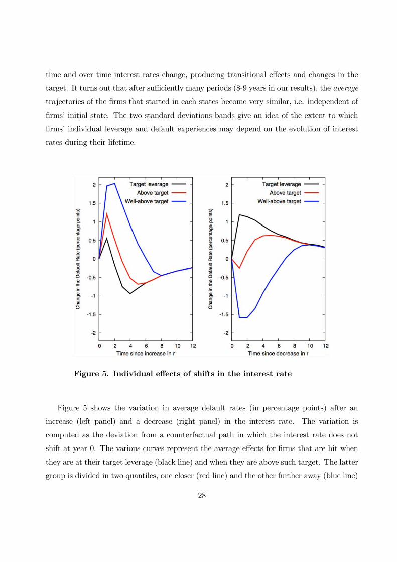
Figure 5. Individual effects of shifts in the interest rate

Figure 5 shows the variation in average default rates (in percentage points) after an

increase (left panel) and a decrease (right panel) in the interest rate. The variation is

computed as the deviation from a counterfactual path in which the interest rate does not

shift at year 0. The various curves represent the average effects for firms that are hit when

they are at their target leverage (black line) and when they are above such target. The latter

group is divided in two quantiles, one closer (red line) and the other further away (blue line)

28

from target leverage. The well-above target group includes the start-ups.

The figure evidences the importance of two key properties of the effects of interest rate

shifts in the model: (i) the heterogeneity in the response across firms and (ii) the asymmetry

in the effects of interest rate rises vs. interest rate cuts. Both are due to the underlying

corporate finance frictions. Following an interest rate rise, firms with higher leverage suffer

more from excessive indebtedness (and high default) in the short-run and take it longer to

adjust to their new, lower leverage target (which eventually implies a lower default rate).

Following an interest rate cut, mature firms adjust to their new, higher target leverage

immediately (which explains the short-term spike in the default rate), while for the youngest

firms the cut implies lowering the burden of their excessive leverage and a quicker convergence

to the now higher (but still lower than what they have) leverage target.

Figure 6. Aggregate effects of changes in the interest rate

Figure 6 shows the implications of aggregating across the whole population of active firms

the effects that we have just commented: it depicts the variation in the aggregate default rate

29

(in percentage points) after an increase (blue line) and a decrease (red line) in the interest

rate. As before, the variation is computed as the deviation from a counterfactual path in

which the interest rate does not shift at year 0. Somewhat surprisingly, in the shortest run

any shift in the risk-free rate has a negative impact on the aggregate default rate. This

reflects that the large default-increasing effect among (the relatively small measure of) non-

mature firms dominates after a rise, while the pretty large default-increasing effect among

(the large measure of) mature firms dominates after a cut. In the longer run, moving to

higher (lower) rates tends to reduce (rise) aggregate leverage and aggregate default.

Figure 7. Aggregate effects under alternative interest rate dynamics

Finally, in order to better understand the effects of aggregate uncertainty, we solve the

model and recompute the effects of interest rate shifts under two alternative parameteriza-

tions of the Markov chain followed by the risk-free interest rate. The two panels in Figure

30

6 compare the effects described in Figure 5 for our baseline parameterization with those

obtained in each of the alternative scenarios. In the left panel, the alternative process fea-

tures larger state persistence (we increase πLL = πHH from 0.9293 to 0.95), while in the

right panel it features smaller differences between the high and the low interest rate (we

increase the low rate to 1% and reduce the high rate to 2.65%, preserving the unconditional

mean). Interestingly, the higher persistence of each phase (which might correspond to the

empirical situations in which interest rates are kept “too low for too long”), exacerbates the

default-increasing effect of interest rates rises in the shortest term, while it dampens the

default-increasing effects of interest rate cuts –possibly because the decrease (increase) in

firms’ continuation value after the shift in the interest rate is larger if rates are expected

to remain high (low) for a longer period. As for the right panel, reducing the amplitude of

interest rates swings reduces the size of both the short and long run effects of each change.

In fact, under the alternative parameterization, the aggregate default-increasing effect of

interest rate rises disappears.

5 Discussion of the results

5.1 Consistency with the literature on firms’ life cycle

To facilitate tractability and the understanding of the mechanisms behind the results, our

model contains assumptions that leave aside many potentially important phenomena re-

garding firms’ life cycle. First, our firms’ size is fixed and all the investment occurs at the

startup period, while real world firms would most typically start small and grow over time.

Second, our firms are ex ante equal, except for the interest rate state faced when they start

up, so they face no explicit process of learning whereby firm quality gets gradually revealed,

reputation or market share build up, or a market discipline mechanism leading to, say, the

survival of the fittest.30

Lastly, our entrepreneurs are penniless when they start up, so 100% of their firms’ initial

funding needs are covered with outside funding. In reality, most firms that start small

30However, one can think of our endogenous survival probabilities, affected by the moral hazard problembetween entrepreneurs and their financiers, as a reduced form for the influence of finance-related incentiveson that type of process.

31

and inexperienced count on significant amounts of inside funding (from the entrepreneurs

or their friends and family) as well as, at least in some sectors, funding from specialized

agents such as angel investors, venture capitalists and other startup incubators (who may

also provide monitoring and advice). In this regards, one might argue that what is described

as entry of “startups” in the model actually refers to a major expansion decision of some

already established firms (i.e. a decision involving a much more sizeable investment than at

their foundation). Under this reinterpretation, we are just normalizing the (marginal) inside

funding available to the firms under consideration to a common value of zero. From this

perspective, the model is more about identifying ceteris paribus implications of interest rate

shifts for the leverage and default of some established firms in the course of expanding than

a full account of firms’ life cycles.

Theoretical work on firms’ life cycles with an emphasis on finance include Cooley and

Quadrini (2001) and Clementi and Hopenhayn (2006), which stress the importance of finance

for growth and survival, but rule out default and do not discuss the implications of interest

rate shifts. Empirical work on firms’ life cycles tends to focus on how firm size and firm

survival evolves with firm age. Our model’s feature regarding firms’ gradual approach to

some target leverage and the decline, ceteris paribus, in their probability of default along such

process is consistent with the higher survival rate of older firms documented by Evans (1987)

and Audretsch (1991), among others. Several papers document the importance of financial

factors (Angelini and Generale, 2008) as well as non-financial factors such as product life

cycles (Agarwal and Gort, 2002) and idiosyncratic profitability shocks (Warusawitharana,

2011). Zingales (1998) offers evidence on the importance of leverage, in addition to individual

efficiency, as a determinant of the probability of firm survival after a sector specific shock.

Our model’s prediction that default probabilities fall with leverage and are lower for dividend-

paying firms (i.e. firms that have already reached their target leverage) is consistent with

the reduced-form results in Jacobson et al. (2011).

On broader grounds, our model is consistent with Kayhan and Titman (2007) and Byoun

(2008), who document the importance of history as a determinant of firms’ capital structure

and their tendency to move towards target debt ratios over time. It is also consistent with

DeAngelo et al. (2006), who document that dividend payments are much more frequent

32

when retained earnings account for a large proportion of total equity, while they fall to near

zero if equity is contributed rather than earned.31

To the best of our knowledge, the few papers that analyze the effect of interest rates

on default probabilities do not explicitly condition the interest rate effects on firm leverage

and do not allow for asymmetric effects of interest rises and cuts. Yet, the effects that we

predict are conceptually consistent with the non-linearities documented by Korajczyk and

Levy (2003) and Halling et al. (2011), who report differences in firms’ target leverage and

speeds of adjustment to their targets across expansions and recessions (and across different

types of firms).32

5.2 Macroprudential implications

If we think of reference risk-free interest rates, possibly affected by monetary policy, as a key

determinant of what the model describes as rt–financiers’ opportunity cost of funds–then

our results have implications for recent discussions on the macroprudential role of monetary

policy. First of all, they provide a call for caution against conclusions reached in static

models, in models without firm heterogeneity, in linear regression models, and whenever the

empirical data contains relatively limited exogenous variation in the empirical counterpart

of rt. Those analyses may miss important aspects of the effects of interest rates on corporate

leverage and credit risk.

According to our analytical results, lower interest rates imply larger target leverage but

may or may not lead to lower default rates. Lower rates make the lending to the highest-

levered firms safer because they reduce these firms’ effective debt burden, but they may

make mature firms riskier, since mature firms will go for higher leverage. Indeed, under our

baseline parameterization of the model, the aggregate default rate is on average higher when

31Our model considers short-term debt as the only source of outside funding, but a similar moral hazardproblem with implications for firms’ survival would emerge if our entrepreneurs were receiving their outsidefunding in the form of contributed equity.32In order to rationalize this evidence one could think of a variation of our model in which fluctuations in

aggregate productivity or aggregate demand are captured by introducing Markov state dynamics in firms’output conditional on success, say yt (currently equal to a constant y). Firms would react to a switch to thelow output state by reducing their target leverage but would experience high leverage and high default riskin the transition to their new target. A switch back to the high output state would increase target leveragebut the transitional effects would not be symmetric to (but shorter and less intense than) those found in theswitch to the low output state.

33

the interest rate is lower. So our results are consistent with the observation that having

interest rates “too low for too long” may imply larger “risk taking” (Borio and Zhu, 2008).

However, we also find that interest rate rises will tend to produce a temporary rise in default

rates, which means that the macroprudential use of monetary policy (e.g. if authorities care

about negative externalities caused by high default rates) involves difficult intertemporal

trade-offs.

Finally, in a model like ours, absent negative externalities associated with a higher de-

fault rate, the equilibrium levels of leverage and default (sometimes interpreted as proxies of

lenders’ risk-taking, especially when they are banks) cannot be properly deemed excessive

from a normative perspective since there would be no welfare gains from constraining entre-

preneurs’ leverage decisions.33 Moreover, in our model, some of the usual proxies for “risk

taking” tend be larger when rt is lower, but the model per se provides no rationale to advo-

cate keeping interest rates artificially high so as to induce lower leverage and lower default

rates. This means that extracting normative macroprudential prescriptions would require

identifying and quantifying negative externalities associated with the equilibrium levels of

leverage and default produced by a model like ours.

6 Conclusions

Monetary policies leading to a long period of (too) low interest rates have been mentioned as

a possible factor contributing to the genesis of the Great Recession of 2008-2009. Wondering

about possible theoretical underpinnings of such a view, this paper develops a dynamic

corporate financing model with the explicit goal of examining the impact of shifts in the risk-

free interest rate on corporate leverage and credit risk. Firms’ financing problem is affected

by two key frictions: a moral hazard between entrepreneurs and their outside financiers and

entrepreneurial wealth constraints. Interest rates enter the problem by determining outside

financiers’ opportunity costs of funds. The endogenous link between leverage and default

33As in other models with financial constraints (e.g. Lorenzoni, 2008), aggregate welfare measures mayincrease using redistributive policies that reduce the constraints of the agents for which they are morebinding. In this economy, one such policy might consist of subsidizing over-indebted firms to speed up theirconvergence to target leverage. But more than constraining firms’ leverage, this policy would consist ontransferring them funds that they would find in their best interest to use to reduce their leverage.

34

risk comes from the lower incentives of overindebted entrepreneurs to guarantee the survival

of their firms.

The need to finance new investment with outside funding pushes firms’ leverage ratio

above some state-contingent target towards which they gradually adjust through earnings

retention. The dynamic response of leverage and default to cut and rises in interest rates

is both asymmetric (since it is easier to adjust to a higher target leverage than to a lower

one) and heterogeneously distributed across firms (since interest rates affect the burden of

outstanding leverage, which differs across firms). We find that both interest rate rises and

interest rate cuts may increase the aggregate default rate in the short-run. Instead, higher

rates produce lower default rates in the longer run since they induce lower target leverage

across all firms. These results help rationalize some of the empirical evidence regarding the

so-called risk-taking channel of monetary policy and are relevant to current discussions on

the potential macroprudential role of monetary policy.

35

Appendix

Proof of Lemma 1 The domain of the value function is made of the values of R for which(1) has a solution. If (1) does not have a solution, the firm gets liquidated and pays a finaldividend of zero. We could extend the definition of the value function for these values of R bymaking v(R) = 0 but in this extended domain the function is constant rather than strictlyincreasing. So we will constrain attention to the domain in which refinancing is feasible.Hence, consider any two values of the state variable, R1 and R2 with R1 < R2 for which (1)has a solution and denote the optimal decisions made under Ri as (pi, bi, R0i). Notice that if(p2, b2, R

02) is a feasible solution under R2, then it is also a feasible solution under R1, since

the only effect of R1 < R2 on the constraints is to make (4) less stringent. However, thevalue of the objective function under R1 when evaluated at the solution (p2, b2, R02) togetherwith the definition of v(R1) implies:

v(R1) ≥ (y + b2 −R1) + β[u(p2) + pv(R02)] = (R2 −R1) + v(R2) > v(R2),

which proves the result.¥

Proof of Proposition 1 The Lagrangian of this problem is:

L = y +B(R0)−R+ β[u(P (R0)) + P (R0)v(R0)] + λ[y +B(R0)−R], (15)

where λ ≥ 0 is the Lagrange multiplier associated to the inequality constraint. By Kuhn-Tucker conditions, the constraint may or may not be binding. If (9) is not binding, thenλ = 0 and the solution for R0 satisfies the following FOC:

B0(R0) + β{[u0(P (R0)) + v(R0)]P 0(R0) + P (R0)v0(R0)} = B0(R0) + βP (R0)v0(R0) = 0, (16)

where we have used the fact that [u0(P (R0))+ v(R0)] = 0 by (5). Interestingly, (16) does notinvolve R, so it yields the same unconstrained solution R0 = R∗ for all the values of R inwhich (9) can be satisfied, that is, for all R ≤ R ≡ y + B(R∗). Notice that in (16) the factthat v0(R0) < 0 for all R0 implies that B0(R∗) > 0, which means (as advanced above) thatR∗ must be in an upward sloping section of B(R0) and we must have R∗ ≤ R.

For R > R, (9) is binding, then λ ≥ 0 and the solution involves choosing the lowestR0 > R∗ that satisfies B(R0) = R−y. Thus, this solution must also be in the upward slopingsection of B(R0). With a single-peaked B(R0) the inverse of its upward sloping section iswell defined, so with slight abuse of notation we can describe the candidate solution asR0 = B−1(R − y). The existence of this candidate solution requires B−1(R − y) ≤ R, i.e.R ≤ y +B(R).

36

The remaining statements contained in the proposition can be immediately derived fromthese results.¥

Proof of Proposition 3 The results stated in this proposition come from the comparativestatics (total differentiation) of a reduced system of equations inR∗ and p∗ and the exogenousparameters which describes the steady state. To obtain such a reduced system, consider firstthe first order condition (16) satisfied by R∗:

B0(R∗)− βP (R∗) = 0. (17)

We want to find out a compact expression of B0(R∗).Particularizing (6) and (5), we have

B(R∗) =1

1 + r[L+ P (R∗)(R∗ − L)], (18)

andu0(P (R∗)) + v(R∗) = 0. (19)

It directly follows from deriving in (18) with respect to R∗ that

B0(R∗) =1

1 + r[P (R∗) + P 0(R∗)(R∗ − L)]. (20)

On the other hand, deriving in (19) with respect to R∗ we have:

u00(P (R∗))P 0(R∗) + v0(R∗) = 0.

But applying the Envelop Theorem on (8) for R = R∗ and taking into account that theconstraint of the stage problem is not binding at that point makes it obvious that v0(R∗) =−1, so we can write

P 0(R∗) =1

u00(P (R∗)),

which substituted into (20) yields

B0(R∗) =1

1 + r

∙P (R∗) +

1

u00(P (R∗))(R∗ − L)

¸,

which plugged into equation (17) and, after some reordering, allows us to write such equationas:

[1− β(1 + r)]P (R∗) +1

u00(P (R∗))(R∗ − L) = 0. (21)

Since β(1 + r) < 1 and u00(·) < 0, satisfying this condition requires R∗ > L, which meansthat the firm will default on its repayment obligation when it fails. The probability of failure

37

is 1 − p∗, which is strictly positive under our assumption that limp→1 |u0(p)| is sufficientlylarge.Now, using the notation v∗ = v(R∗), p∗ = P (R∗), and b∗ = B(R∗), we can characterize

the steady state as the solution to the system of the following four equations with fourunknowns (namely p∗, b∗, R∗ and v∗):

v∗ = y + b∗ −R∗ + β[u(p∗) + p∗v∗], (22)

−[1− β(1 + r)]p∗u00(p∗)− (R∗ − L) = 0, (23)

b∗ =1

1 + r[L+ p∗(R∗ − L)], (24)

u0(p∗) + v∗ = 0. (25)

In this system, (22), (23), (24), and (25) are the counterparts of (1), (21), (18), and (19),respectively.Finally, using (24) to substitute for b∗ in (22), and (25) to also substitute for v∗ in (22),

the system simplifies to:

H1( p∗, R∗; β, r, y, L+ + − + − −

) ≡ −(1−βp∗)u0(p∗)−y+(1− p∗

1 + r)R∗− 1− p∗

1 + rL−βu(p∗) = 0,

H2( p∗, R∗; β, r, L+ − − − +

) ≡ −[1− β(1 + r)]p∗u00(p∗)− (R∗ − L) = 0,

where the only unknowns are p∗ and R∗, and the signs below each of the arguments ofthe functions H1 and H2 indicate the sign of the corresponding partial derivative. Theremaining results in the proposition come from fully differentiating this system with respectto p∗, R∗, and the exogenous parameters. Signing most of the results is immediate. Only afew require some cumbersome algebra that we skip for brevity. To sign some of the partialderivatives, it is important to remember two properties implicit in our formulation: (i) R∗

is necessarily in the upward slopping section of B(R∗), so we must have B0(R∗) ≥ 0, whichimplies −p∗u00(p∗) ≥ (R∗ − L), (ii) the (iso-elastic) form of u(·) adopted in (13) satisfies−pu000(p)/u00(p) = 2− α and, hence, is smaller than 1 for all α > 1.¥

Proof of Proposition 4 The results stated in this proposition come from the comparativestatics (total differentiation) of a reduced system of equations that, for each given value ofR > R, gives the value R0 = B−1(R − y) that describes the upward slopping section ofthe phase diagram depicted in Figure 1, as well as the continuation probability p = P (R0)associated with that constrained level of leverage. Going back to the definitions of B(R0)

38

and P (R0) in terms of more fundamental ingredients of the model, it is convenient to think ofthe relevant p and R0 as determined by the system of three equations with three unknowns(with b = B(R0) as the third unknown) given by the binding constraints of the originaloptimization problem in (1):

u0(p) + v(R0) = 0, (26)

L+ p(R− L)− (1 + r)b = 0, (27)

y + b−R = 0, (28)

where (26) is (2) written as in (5), (27) corresponds to (3), and (28) is the binding version of(4). Clearly we can use (28) to substitute for b in (27), and arrive to a two-equation systemthat can be written as:

J1( p, R0; β, r, y, L− − + − + +

) ≡ u0( p−) + V ( R0; β, r, y, L

− + − + +) = 0, (29)

J2( p, R0; R, r, y, L+ + − − + +

) ≡ L+ p(R− L)− (1 + r)(R− y) = 0, (30)

where we have written v(R0) = V (R0;β, y, L, r) to make clear that the continuation valueof the firm, as determined by the Bellman equation (1) is a function of the state variableas well as all the underlying parameters. The signs below each of the arguments of thefunctions J1 and J2 indicate the sign of the corresponding partial derivatives, most of whichare immediate to obtain. Notice that the partial derivatives of the function V (R0;β, y, L, r)can be obtained using (1), the Envelop Theorem, and the fact that any parameter thattightens a binding constraint will reduce the value resulting from the maximization.Equations describe two curves and the constrained optimal refinancing decision given R

is given by the intersection between them. To obtain the results stated in the proposition,notice that (29) implicitly defines an decreasing relationship between p and R0 which can becompactly described as

p = P ( R0; β, r, y, L− + − + +

), (31)

and substituted into (30) to obtain:

K( R0; β, R, r, y, L+ + − − + +

) ≡ J2(P (R0;β, r, y, L), R0;R, r, y, L) = 0. (32)

The signs of the partial derivatives shown in (32) can be determined using the fact thathaving a strictly increasing relationship between R and R0 as in the phase diagram in Figure

39

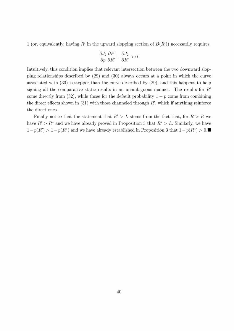
1 (or, equivalently, having R0 in the upward slopping section of B(R0)) necessarily requires

∂J2∂p

∂P

∂R0+

∂J2∂R0

> 0.

Intuitively, this condition implies that relevant intersection between the two downward slop-ping relationships described by (29) and (30) always occurs at a point in which the curveassociated with (30) is stepper than the curve described by (29), and this happens to helpsigning all the comparative static results in an unambiguous manner. The results for R0

come directly from (32), while those for the default probability 1− p come from combiningthe direct effects shown in (31) with those channeled through R0, which if anything reinforcethe direct ones.Finally notice that the statement that R0 > L stems from the fact that, for R > R we

have R0 > R∗ and we have already proved in Proposition 3 that R∗ > L. Similarly, we have1−p(R0) > 1−p(R∗) and we have already established in Proposition 3 that 1−p(R∗) > 0.¥

40

References

Adrian, T., and H. Shin (2010): “Financial Intermediaries and Monetary Economics,” in B.Friedman and M. Woodford (eds.), Handbook of Monetary Economics, vol. 3, Elsevier,601-650.

Agarwal, R. and M. Gort (2002): “Firm and Product Life Cycles and Firm Survival,”American Economic Review Papers and Proceedings, 92, 184-190.

Altunbas, Y., L. Gambacorta, and D. Marqués-Ibañez (2010): “Does Monetary PolicyAffect Bank Risk-Taking?,” BIS WP No. 298.

Angelini, P., and A. Generale (2008): “On the Evolution of Firm Size Distributions,”American Economic Review, 98, 426-438.

Audretsch, D. B. (1991): “New-Firm Survival and the Technological Regime,” Review ofEconomics and Statistics, 73, 441-50.

Kayhan, A., and S. Titman (2007): “Firms’ Histories and Their Capital Structures,” Jour-nal of Financial Economics, 83, 1-32.

Bernanke, B., M. Gertler and S. Gilchrist (1999): “The Financial Accelerator in a Quantita-tive Business Cycle Framework,” in John Taylor andMichael Woodford, eds., Handbookof Macroeconomics, Elsevier, Chapter 21, 1341-1393.

Blume, M. E., F. Lim, and A. C. Mackinlay (1998): “The Declining Credit Quality of U.S.Corporate Debt: Myth or Reality?” Journal of Finance, 53, 1389-1413.

Bolton, P., and X. Freixas (2006): “Corporate Finance and the Monetary TransmissionMechanism,” Review of Financial Studies, 19, 829-870.

Borio, C., and H. Zhu (2008): “Capital Regulation, Risk-Taking and Monetary Policy: aMissing Link in the Transmission Mechanism?,” BIS Working Paper No. 268.

Byoun, S. (2008): “How and When Do Firms Adjust Their Capital Structures towardTargets?,” Journal of Finance, 63, 3069-3096.

Carlstrom, C., and T. Fuerst (1997): “Agency Costs, Net Worth and Business Fluctuations:A Computable General Equilibrium Analysis,” American Economic Review, 87, 893-910.

41

Clementi, G. L., and H. A. Hopenhayn (2006): “A Theory of Financing Constraints andFirm Dynamics,” Quarterly Journal of Economics, 121, 229-265.

Cooley, T. F., and V. Quadrini (2001): “Financial Markets and Firm Dynamics,” AmericanEconomic Review, 91, 1286-1310.

Cooley, T. F., and V. Quadrini (2006): “Monetary Policy and the Financial Decisions ofFirms,” Economic Theory, 27, 243-270.

Cover, J. P. (1992): “Asymmetric Effects of Positive and Negative Money-Supply Shocks,”Quarterly Journal of Economics, 107, 1261-82.

DeAngelo, H., L. DeAngelo, and R. Stulz (2006): “Dividend Policy and the Earned/ContributedCapital Mix: A Test of the Lifecycle Theory,” Journal of Financial Economics, 81, 227-254.

DeMarzo, P. M., and M. J. Fishman (2007): “Optimal Long-Term Financial Contracting,”Review of Financial Studies, 20, 2079-2128.

Dyck, A., and L. Zingales (2004): “Private Benefits of Control: An International Compar-ison,” Journal of Finance, 59, 537-600.

Evans, D. S. (1987): “Tests of Alternative Theories of Firm Growth,” Journal of PoliticalEconomy, 95, 657-74.

Gertler, M., and N. Kiyotaki (2010): “Financial Intermediation and Credit Policy in Busi-ness Cycle Analysis,” in B. Friedman and M. Woodford (eds.), Handbook of MonetaryEconomics, vol. 3, Elsevier, 547-599.

Hackbarth, D., J. Miao, and E. Morellec (2006): “Capital Structure, Credit Risk, andMacroeconomic Conditions,” Journal of Financial Economics, 82, 519-550.

Halling, M., J. Yu, and J. Zechner (2011): “Leverage Dynamics over the Business Cycle,”University of Vienna, mimeo.

Hamilton, J. D. (1989): “Analysis of Nonstationary Time Series and the Business Cycle,”Econometrica, 57, 357-384.

Hennessy, C. A., and T. M. Whited (2005): “Debt Dynamics,” Journal of Finance, 60,1129-1165.

42

Holmstrom, B., and J. Tirole (1997): “Financial Intermediation, Loanable Funds, and theReal Sector,” Quarterly Journal of Economics, 112, 663-91.

Ioannidou, V. P., Ongena, S. and J.-L. Peydró (2009): “Monetary Policy, Risk-Taking andPricing: Evidence from a Quasi Natural Experiment,” European Banking Center DP2009-04, September.

Jacobson, T., J. Linde, and K. F. Roszbach (2011): “Firm Default and Aggregate Fluctu-ations,” Federal Reserve Board International Finance DP 1029, July.

Jiménez, G., S. Ongena, J.-L. Peydró and J. Saurina (2011): “Hazardous Times for Mon-etary Policy: What do Twenty-Three Million Bank Loans Say About the Effects ofMonetary Policy on Credit Risk?,” ECB, mimeo.

Kiyotaki, N., and J. Moore (1997): “Credit Cycles,” Journal of Political Economy, 105,211-248.

Korajczyk, R., and A. Levy (2003): “Capital Structure Choice: Macroeconomic Conditionsand Financial Constraints,” Journal of Financial Economics, 68, 75-109.

Landier, A., D. Sraer , and D. Thesmar (2010): “Going for Broke: New Century FinancialCorporation, 2004-2006,” Toulouse School of Economics, mimeo.

Lorenzoni, G. (2008): “Inefficient Credit Booms,” Review of Economic Studies, 75, 809-833.

Maddaloni, A., and J.-L. Peydró (2011) “Bank Risk-Taking, Securitization, Supervision andLow Interest Rates: Evidence from the Euro Area and the U.S. Lending Standards,”Review of Financial Studies, 24, 2121-2165.

Mankiw, G. (1986): “The Allocation of Credit and Financial Collapse,” Quarterly Journalof Economics, 101, 455-470.

Molina, C. (2005): “Are Firms Underleveraged? An Examination of the Effect of Leverageon Default Probabilities,” Journal of Finance, 60, 1427-1459.

Morellec, E., B. Nikolov, and N. Schurhoff (2010): “Corporate Governance and CapitalStructure Dynamics,” Journal of Finance, forthcoming.

Rajan, R. G. (2005): “Has Financial Development Made the World Riskier?,” NBERWork-ing Paper 11728.

43

Repullo, R., and J. Suarez (2000): “Entrepreneurial Moral Hazard and Bank Monitoring:A Model of the Credit Channel,” European Economic Review, 44, 1931-1950.

Shleifer, A., and R. W. Vishny (2010): “Unstable Banking,” Journal of Financial Eco-nomics, 97, 306-318.

Stiglitz, J. E., and A. Weiss (1981): “Credit Rationing in Markets with Imperfect Informa-tion,” American Economic Review, 71, 393-410.

Tirole, J. (2005): The Theory of Corporate Finance, Princeton University Press.

Warusawitharana, M. (2011): “Profitability and the Lifecycle of Firms,” Federal ReserveBoard, mimeo. Available at SSRN: http://ssrn.com/abstract=1568965.

Weise, C. L. (1999): “The Asymmetric Effects of Monetary Policy: A Nonlinear VectorAutoregression Approach,” Journal of Money, Credit, and Banking, 31, 85-108.

Williamson, S. D. (1987): “Costly Monitoring, Loan Contracts, and Equilibrium CreditRationing,” Quarterly Journal of Economics, 102, 135-146.

Zingales, L. (1998): “Survival of the Fittest or the Fattest? Exit and Financing in theTrucking Industry,” Journal of Finance, 53, 905-938.

44