Interactive Sustainable Blueberry Budget

User Guide

1

Interactive Sustainable Blueberry Budgets: User Guide

CONTRIBUTING AUTHORS

Dr. Hector German Rodriguez, Research Program Associate of Agricultural Economics & Agribusiness, University of Arkansas Dr. Jennie Popp, Professor of Agricultural Economics & Agribusiness, University of Arkansas Sokha Sok, Graduate Student of Agricultural Economics & Agribusiness, University of Arkansas Dr. Elena Garcia, Fruit and Nut Extension Specialist, University of Arkansas System Division of Agriculture TABLE OF CONTENTS INTRODUCTION ................................................................................................................................................................ ....... 2

SOFTWARE REQUIREMENTS ............................................................................................................................................. 3

QUICK START GUIDE.............................................................................................................................................................. 3

GETTING STARTED ................................................................................................................................................................ . 4

1. INITIAL INPUT ................................................................................................................................................................ 4

2. NAVIGATING AND EDITING DEFAULT VALUES ............................................................................................. 11

3. ECONOMICS ................................................................................................................................................................ .... 13

3.1. Breakeven Analysis ........................................................................................................................................... 16

3.2. Sensitivity Analysis ............................................................................................................................................ 19

3.3. Risk Analysis ........................................................................................................................................................ 21

4. HELP AND OTHER TOPICS ....................................................................................................................................... 23

5. GLOSSARY ....................................................................................................................................................................... 24

6. ADDITIONAL RESOURCES........................................................................................................................................ 26

ACKNOWLEDGEMENTS ...................................................................................................................................................... 26

CONTACT US ............................................................................................................................................................................ 26

REFERENCES ........................................................................................................................................................................... 27

DISCLAIMER ............................................................................................................................................................................ 27

2

INTRODUCTION

The demand for blueberries still typically exceeds supply in much of the state of Arkansas, particularly early and late in the production season. In general, production of berries is considered to be risky because of a high initial investment, a delay of three or more years in returns after planting, the climate (weather extremes), and high fixed costs (Funt et al., 2011). The capital and cash input costs associated with growing blueberries in Arkansas are substantial. Detailed planning is necessary when budgeting for capital expenditures and for the annual operating costs. With new advances in high tunnel technologies, Arkansas growers have more opportunities to extend the blueberry season to meet the year-round demand while avoiding the need to ship long distances, thus leaving a lighter environmental footprint by minimizing fuel consumption.

The budget presented here should be used as a guide only, as individual on-farm production systems may have higher or lower costs and revenues than those listed. The budget is divided into variable costs (plants, fertilizers, insecticides, hours of labor, etc.), fixed costs (machinery and equipment, irrigation, high tunnel systems (if any), taxes, insurances, land costs, management, etc.), and total costs (variable costs plus fixed costs). If the farm is not entirely dedicated to blueberry production, the fixed costs should be allocated proportionally among all crops to obtain a more accurate budget. Net returns are calculated by subtracting total costs from gross returns (yield times price) each year. Since the budget is developed for a long period of time (seven years), it is necessary to adjust future returns to today’s dollars. Money today is typically worth more than money in the future because of inflation.

Production costs and yields on each operation differ due to soil type, climatic conditions and agronomic practices, among others reasons. The price producers receive is determined by the market strategy chosen by the producer, quality of the product, supply of fruit in the area and other unique characteristics specific to each production situation. Therefore, producers are encouraged to enter their own values to develop their own cost of production for their specific blueberry production.

The purpose of this tool is twofold: 1) to assist producers in the evaluation of costs, revenues and risks associated with their blueberry operation, and 2) to assess the changes to cost, revenue and risk as expected costs, revenue prices and/or yields change. The production budget components of the tool estimate gross revenues, variable costs, fixed costs and total net returns using the tool’s default data or information entered by the user.

3

But what makes this tool unique is that it includes additional economic components not found in most production budgets that: 1) estimate the operation’s breakeven price and yield, 2) conduct sensitivity analyzes (answering “What if” questions related to changes in costs and revenues), and provide a risk assessment (regarding the probability of obtaining positive net returns during the life of the blueberry crop).

This tool is useful because it allows blueberry producers to estimate operating costs, fixed costs, total costs and expected total returns by modifying production practices or production systems, cost or return values. Estimating total costs per year, breakeven analyses for yields and prices, sensitivity analyses for total costs, and risk analyses would assist blueberry producers to make better investment and management decisions when using high tunnels in their operations.

SOFTWARE REQUIREMENTS

This tool employs standard Microsoft Windows graphical elements so that anyone familiar with the Microsoft Windows environment should find this blueberry budget easy to navigate. Familiarity with the basics of mouse operation and navigating standard Windows objects such as menus, windows, dialog boxes, scroll bars, and toolbars is very important in using this tool.

Your personal computer should have the following programs installed and operating properly:

Windows operating system Microsoft Excel version 2007 or higher

QUICK START GUIDE

For easy use, please take a few moments to read the following steps:

1. Press “User Input” 2. Select between field and high tunnel production (Conventional and Organic) 3. Enter or select values in the boxes 4. Click “Run” to see an overview of cost/returns 5. Navigate the application by clicking on icons at the top/bottom of the screen 6. Enter new values to customize the budget 7. Click the “Economics” button to see graphical representations of the data

4

GETTING STARTED

This complete user guide covers everything you need to know to start using this tool. This decision support tool is both easy to use and highly customizable. Before you can use this tool for estimating basic revenue calculations, you must tell the program a few things about your current or potential operation. Please open the tool now and follow the instructions below.

1. INITIAL INPUT

Figure 1 shows the “Cover” screen. It explains what the tool does. Click “Start” to continue.

Figure 1. Cover Menus – Blueberry Budget

From the “Main Menu” screen you can navigate across the tool (Figure 1.1).

5

Figure 1.1 Main Menu Screen

Click on any of the green icons to get more information about this tool. Detailed instructions are available by clicking on the “User Guide” icon or by following the steps in the “Quick Start” to start using this application. Figure 2 shows the userform where you can select any of the four production systems that you can estimate with this tool.

6

Figure 2. Choosing a Production System

Four different user-forms will appear depending on your selection. If you click on “Conventional field production”, a userform will display nine questions (Figure 3).

Figure 3. Conventional Field Production Userform

7

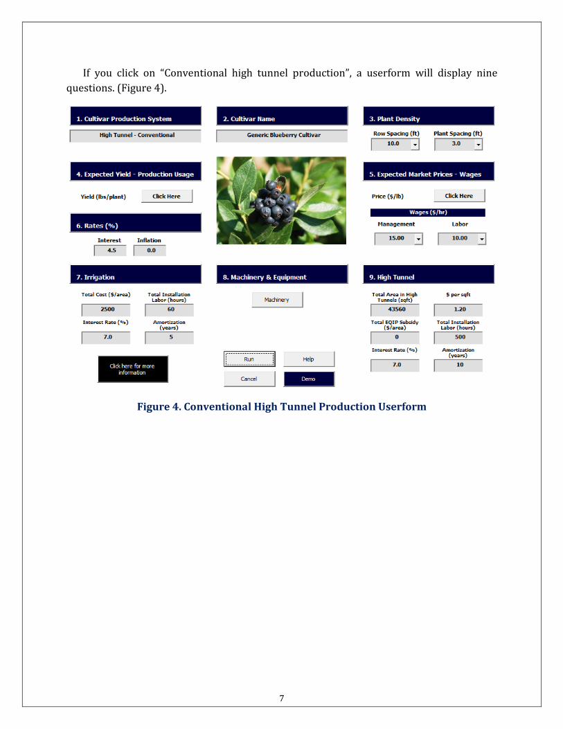
If you click on “Conventional high tunnel production”, a userform will display nine questions. (Figure 4).

Figure 4. Conventional High Tunnel Production Userform

8

Click on each of the boxes to enter your own values. All the information in the boxes is required to calculate the budget. The user-form will open with default values; you can overwrite these values with your own information at any time. Warning messages will appear if there is missing information or if you enter invalid input. Figure 5 shows an example of a warning message related to missing information.

Figure 5. Example of Warning Messages

The model can be run quickly by clicking the demo button. This will populate the tool with all needed information. However, in order to customize this tool to your own operation, follow these steps. Please note information for all categories marked with an “*” is needed for the tool to run.

1. Fruiting Cultivar Production System – This is the production system that you have

chosen.

2. Cultivar Name – Enter cultivar name.

3. *Plant Density (plant/ac.) – Enter the planting distance in both “In Row (ft.)” and “Between Rows (ft.)” boxes. Once both values have been entered, the tool will automatically calculate the number of plants per acre.

4. *Yield (lb. /plant) and Production Usage (%) – Enter expected yields per plant per

year as well as “Fresh Market” and “Processed Market” percentages for the first seven years. These two percentages must be equal to 100% or less. If the total of both percentages is greater than 100%, a message will appear asking to correct your input. If the total of both percentages is less than 100%, it is assumed that the difference is culled fruit.

9

5. *Market Price ($/lb.) and Wages ($/hr.) – Enter the expected prices for “Fresh Market” and “Processed Market” fruit for each year.

6. *Rates (%) – enter interest and inflation rates.

7. *Field Production Area (Only field production) – enter area in acres (e.g., 0.3, 0.5, 1.0,

1.5, 2.0, etc.)

8. Machinery & Equipment – Enter machinery or equipment name, purchase cost, ownership life, salvage value (e.g., usually 20%), ownership tax costs, ownership shelter costs, and ownership insurance costs. If there is incomplete information, a message will let you know what information is missing and will take you to the corresponding box. If you do not enter the name of the machinery or equipment but you enter information in the other columns, that row information will not be included in the final calculations. Once you enter your machinery and equipment properly, you need to enter the hours of annual use for each machinery and equipment. You need to enter hour usage information for at least one of the seven years. Click on the “Demo” icon if you want to use the default values. Rental equipment can be entered each year after running the model.

9. Irrigation System – Enter your irrigation system information (e.g., total costs,

installation labor hours, interest rate and amortization period, in years).

10. High Tunnel – Enter the size of your high tunnel (in square feet), the costs per square foot, value of the total EQIP subsidy (If any), the number of labor hours to install the high tunnel, the interest rate (%) for your loan and the number of years to pay the loan. This information is required if you decided to use a high tunnel in your operation. This information does not apply for field production.

10

By clicking on the “Run” icon, the tool will check if there is missing information. If the initial input was not entered correctly or there is missing information, a warning message asking you to correct the data will appear. If there is no missing information, the tool will open to the “Economics” screen to show a graphical representation of the budget as in Figure 6.

Figure 6. Economics Screen

11

From the “Economics” screen you can access the “Summary” screen (Figure 6.1). This screen is a snapshot of all production activity costs (variable and fixed cots), gross revenues and net returns. From this screen you can navigate across 15 different years (e.g., soil preparation, establishment, growth, and year one to 12 of production) to modify or to enter new information. In addition, you can return to the main menu, access the economic tools, access the user guide, obtain help, or edit your initial input.

Figure 6.1 Summary Screen

2. NAVIGATING AND EDITING DEFAULT VALUES

You can navigate across this tool from virtually any screen. There are navigation icons on each screen that enables movement across screens to edit, update or view information (Figure 7). Click any icon on the “Navigation Tool”, to quickly move among the various screens. In these screens, you can modify, update or enter new information. The blue icon with the text in yellow will indicate in which screen you are at the moment.

Figure 7. Example Navigation Icons on the Navigation Tool

Navigating to any category screen will reveal detailed descriptions of the costs of

production for each activity and the price and quantity values used to make the calculations. You may enter your own values by placing new values in the “Your Quantity” or “Your Price” columns. Once any new values are entered, calculations are automatically

12

updated. If you modify the default values, the total costs will be highlighted in green. This helps to identify the activities that were modified (Figure 8).

This tool calculates costs and revenues based on a representative set of activities that occur in any given year on a blueberry crop. Additional activities specific to a producer’s operation can be added to the budget; just enter a name or description, unit, quantity, and price per unit. The total cost per each additional activity will be calculated automatically. Values will be highlighted in blue.

Figure 8. Modifying Default Values

13

3. ECONOMICS

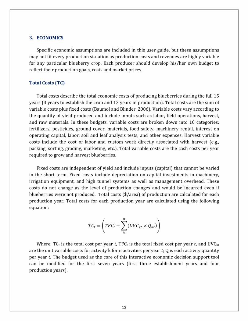
Specific economic assumptions are included in this user guide, but these assumptions may not fit every production situation as production costs and revenues are highly variable for any particular blueberry crop. Each producer should develop his/her own budget to reflect their production goals, costs and market prices. Total Costs (TC)

Total costs describe the total economic costs of producing blueberries during the full 15 years (3 years to establish the crop and 12 years in production). Total costs are the sum of variable costs plus fixed costs (Baumol and Blinder, 2006). Variable costs vary according to the quantity of yield produced and include inputs such as labor, field operations, harvest, and raw materials. In these budgets, variable costs are broken down into 10 categories; fertilizers, pesticides, ground cover, materials, food safety, machinery rental, interest on operating capital, labor, soil and leaf analysis tests, and other expenses. Harvest variable costs include the cost of labor and custom work directly associated with harvest (e.g., packing, sorting, grading, marketing, etc.). Total variable costs are the cash costs per year required to grow and harvest blueberries.

Fixed costs are independent of yield and include inputs (capital) that cannot be varied

in the short term. Fixed costs include depreciation on capital investments in machinery, irrigation equipment, and high tunnel systems as well as management overhead. These costs do not change as the level of production changes and would be incurred even if blueberries were not produced. Total costs ($/area) of production are calculated for each production year. Total costs for each production year are calculated using the following equation:

𝑇𝑇𝑡 = �𝑇𝑇𝑇𝑡 + �(𝑈𝑈𝑇𝑘𝑡 × 𝑄𝑘𝑡)𝑛

𝑘

�

Where, TCt is the total cost per year t, TFCt is the total fixed cost per year t, and UVCkt

are the unit variable costs for activity k for n activities per year t; Q is each activity quantity per year t. The budget used as the core of this interactive economic decision support tool can be modified for the first seven years (first three establishment years and four production years).

14

Gross Revenues (GR)

Gross revenues are estimated by multiplying expected market price ($/lb.) for each fruit quality (e.g., Quality 1 or Quality 2) and expected yield (lb./area) for each fruit quality for each year of production. Annual gross revenues of production are calculated for each production year t using the following equation:

𝐺𝐺𝑡 = ��𝑌𝐸𝐸𝐸𝑡 × 𝑃𝐸𝐸𝐸𝑡� + �𝑌𝐸𝐸𝐸𝑡 × 𝑃𝐸𝐸𝐸𝑡��

Where, GR is the expected gross revenues per year t, YEFM is the expected yield to be

sold in the fresh market (e.g., Quality 1) in year t, PEFM is the expected price to be received for fresh market fruit in year t, YEPM is the expected yield to be sold in the processing market in year t, PEPM is the expected price to be received for processing fruit (e.g., Quality 2) in year t. Expected yields for each fruit quality are estimated as follows:

𝑌𝐸𝐸𝐸𝑡 = (𝑇𝑌𝑡 × 𝐸𝑇𝐸𝑡) × 𝑇𝑇

𝑌𝐸𝐸𝐸𝑡 = (𝑇𝑌𝑡 × 𝐸𝑃𝐸𝑡) × 𝑇𝑇

Where, TY is the expected total yield per year t, EFM is the expected percentage of

quality 1 produced in year t, EPM is percentage of processed market fruit produced in year t, TA is the total number of plants per area. All these yield values are input that the user needs to enter and can be modified or changed at any time. It is important to point out that there will always be some percentage of culls or drops. The user can enter expected quality 1 and quality 2 percentages for each year of production. These two percentages must be equal to 100% or less each year. If the total of both percentages is greater than 100%, a message will appear asking to correct the input. If the total of both percentages is less than 100%, it is assumed that the difference is culled fruit. Net Returns (NR)

Net returns ($/area) are estimated each year by subtracting total cost ($/area) from gross revenues ($/area). Net returns for each production year t (NRt) are calculated using the following equation:

𝑁𝐺𝑡 = 𝐺𝐺𝑡 − 𝑇𝑇𝑡

15

Future Values (FV)

The blueberry budget could be used by a producer to estimate costs and revenues across the life of a blueberry crop before determining whether or not to undertake the operation. However, all future costs and revenues are unknown. One way to estimate the values of costs and revenues that occur in the future is to increase current values annually by an expected inflation rate using the following equation:

𝑇𝑈𝑡 = 𝑃𝑈𝑡 × (1 + 𝐼)

Where, FV is future cash flows occurring at time t, PV is the present value (explained below) and I is the inflation rate in decimal form. Present Values (PV)

Present value is a future amount of money that has been discounted (using an average discount rate) to reflect its current value, as if it existed today. Present value calculations are used to make comparisons between cash flows and production years, as they do not occur at simultaneous times (Baumol and Blinder, 2006). The soil preparation year is assumed as the starting year (t=0). After this year, all the calculations are adjusted by the average discount rate to estimate present values. Present values for variable and fixed costs, gross revenues and net returns were estimated using the following equation:

𝑃𝑈 = ��𝑇𝑈𝑡

(1 + 𝑑)𝑡�𝑛

𝑡=1

Where, PV, is the present value of future cash flows (FV) occurring at time t, that must

be discounted over the course of n years using d, the discount rate.

Net present value (NPV) was used to estimate the profitability of a blueberry crop that lasts 15 years (3 years to establish, 12 years in production) as annual net returns (gross revenue – total costs) are discounted to the present. Hence, the PV of future net returns received over the life of the crop represents the sum total of profitability expressed in today’s dollars for making the decision to invest in the crop

𝑁𝑃𝑈 = ��𝑁𝐺𝑡

(1 + 𝑑)𝑡�15

𝑡=1

16

Where, NPV is the net present value, NR is the net returns, t is time period and d is the discount rate for one compounding period (in this case, annually).

The inflation rate (I) is used to adjust the value of future cash flows. Then the discount rate (d) is used to determine the PV of future cash flows. Both of these rates are entered by the user and can be updated at any time. Note that year 0 is included to represent cash flows occurred in the soil preparation year that need not be discounted. The PV of net returns or NPV is used in the risk assessment component of this budget. The larger the NPV, the better is the investment (Baumol and Blinder, 2006). Given our assumptions, a negative NPV implies that total costs cannot be covered using revenue streams generated by the crop.

By clicking on the “Economics” icon (from any screen), a graphical representation of the

total cost of production, gross revenues, and net returns per area associated with the information entered in the “User Input” form and all the other screens will be displayed (See Figure 6). This tool will calculate breakeven points for price and yield (see Breakeven Analysis for more information). Sensitivity and Risk analyses can also be conducted (see Sensitivity and Risk Analyses for more information).

Depreciation (Amortization)

There are two categories (e.g., Irrigation and High Tunnel) depreciated in this tool. The

user must enter the total costs, the total number of hours used to install the system, an interest rate and the duration of the loan in years as an initial input. The total value of the each system is broken down to the number of years the system is expected to operate based on the initial information entered. The total cost of the labor hours spent in the installation of a system is not used in the depreciation of the system. That costs is assumed to be a variable costs in the establishment year.

3.1. Breakeven Analysis

Although obtaining positive net present values is the main goal, it is very important to know if/when the production of blueberries will cover the total costs of production or, in other words, breakeven. This tool calculates how much revenue is needed (given expected “Quality 1” and “Quality 2” yields and prices) to cover the total costs of production.

The breakeven point is defined in this blueberry application as the point at which total costs and total revenues are equal. There is no net loss or gain (i.e., the operation has "broken even"). Expected market production (EMPi) is equal to market yield (EMYi) per plant times the number of plants (NP) per area times expected market price (EMPri), t is

17

time in years, and i is “Quality 1” or “Quality 2” (see market production equation). Total revenues are the sum of expected “Quality 1” or “Quality 2” market production during the life of the crop.

𝐸𝑀𝑀𝑀𝑀𝑀 𝑃𝑀𝑃𝑑𝑃𝑃𝑀𝑃𝑃𝑃 (𝐸𝐸𝑃)𝑖 = �(𝐸𝐸𝑌𝑖 ∗ 𝑁𝑃 ∗ 𝐸𝐸𝑃𝑀𝑖)

So, the breakeven yield (see breakeven yield equation) is calculated by dividing the

cumulative total costs of operating the crop (CTC) by the expected average market price (EMPi) times the ratio between expected market production (EMPi) and total revenues (TR).

𝐵𝑀𝑀𝑀𝑀𝑀𝐵𝑀𝑃 𝑌𝑃𝑀𝑌𝑑𝑖 =𝑇𝑇𝑇𝐸𝐸𝑃𝑖

∗ �𝐸𝐸𝑃𝑖𝑇𝐺

�

The tool will calculate the breakeven “Quality 1” or “Quality 2” yields. For example,

using the tool’s default values for conventional field production, cumulative total costs (CTC) are equal to $63,344/area; total revenues are equal to $121,260/area; “Quality 1” fruit is $2.67/lb. assuming 70% of the fruit is sold in the fresh market and “Quality 2” fruit is $1.00/lb. assuming 30% of the fruit is sold in the processed market. The crop will breakeven (e.g., net returns equal to zero), if total production is equal to 75,861 pounds.

Likewise, the breakeven price (see breakeven price equation) is calculated by dividing

the cumulative total costs of operating the crop (CTC) by the expected average market yield (EMYi) times the ratio between expected market production (EMPi) and total cumulative revenues (TR). The resulting numbers will be the average annual price per pound (for each quality) that must be attained for blueberries sold for exactly zero profit to be obtained at the end of the year.

𝐵𝑀𝑀𝑀𝑀𝑀𝐵𝑀𝑃 𝑃𝑀𝑃𝑃𝑀𝑖 =𝑇𝑇𝑇𝐸𝐸𝑌𝑖

∗ �𝐸𝐸𝑃𝑖𝑇𝐺

�

For example, using the tool’s default values, cumulative total costs (CTC) are equal to $63,344/area; total cumulative revenues are equal to $121,260/area; total yield is 75,861 lb./area. The crop will breakeven at the end of the year (e.g., net returns equal to zero), if the “Quality 1” (fresh market) price is $0.92/lb. and “Quality 2” (processed market fruit) price is $0.35/lb. By clicking on the “Breakeven Analysis” icon on the Economics page (see

18

Figure 6), a userform will ask to choose between yield and price breakeven points (e.g., net returns equal to zero - see Figure 9).

Figure 9. Breakeven Analysis

A breakeven yield analysis summary is shown in Figure 9.1. All these values are

interactive and will be updated automatically if any input (including expected prices and expected yields) is changed.

Figure 9.1. Example of Yield Breakeven Analysis

19

3.2. Sensitivity Analysis

This tool also allows producers to examine “What If” scenarios to make better planning and investing decisions. A “What If” analysis is also called a sensitivity analysis. This technique is used to determine how different values of an input will impact the final product. In other words, a sensitivity analysis is a way to predict the outcome of a decision if a situation turns out to be different from the current situation. Here, a user might like to know how the cumulative total costs, gross revenues, and net returns will be affected if a change occurs (for example, unexpected lower yields, lower prices, etc.).

The “Sensitivity Analysis” icon (e.g., “What If Analysis”) is located on the right side of the “Economics” screen (Figure 6). Clicking on that icon will load the Sensitivity Analysis Userform (Figure 10). Values for one or more inputs (related to yields, production usage or prices) can be changed to conduct a “What If” analysis. Once the desired values have been changed, a new breakeven analysis as well as new values for cumulative gross revenues and net returns will be calculated. This “What If” analysis presents instantly the impact of a change in one or more of the inputs on the economic feasibility of the whole blueberry crop.

Figure 10. Sensitivity Analysis Userform

20

Figure 10.1 displays the available analysis options from which the user can choose.

Figure 10. 1 Sensitivity Analysis Options

Additionally, the tool will estimate the net returns for different fluctuations (+/- 25% by 5% intervals) from the average for yield and prices (Figure 10.2).

Figure 10. 2 Sensitivity Analysis – Net Returns ($/ac) Yield Fluctuations

21

3.3. Risk Analysis

This tool includes a risk analysis component. In this tool, risk analysis is defined as a technique that calculates the probability of obtaining a cumulative net return greater than a specific dollar target (e.g., $75,000). This target is set by the user. To access the risk analysis component, click the "Risk Analysis" icon located in the “Economics” screen (bottom right corner, see Figure 6). The form will open with default values but they can be changed at any time (Figure 11).

Enter new “minimum”, “most likely” and “maximum” values for yield (lb./plant) and

prices ($/lb.). Enter the percentage of usage for each quality each year. Enter the percentage by which the total cost should increase or decrease each year, a net return target dollar amount ($/area) that you expect to receive at the end of the 15 years of production. After all the input information is recorded, click “Run”.

Figure 11. Risk Analysis Userform

The model will calculate the probability of the net returns value being equal or greater

than a specific dollar target; in this example $75,000. To do this, the model will simulate 1,000 iterations to gain a better understanding of the range of possible cumulative net returns. It also calculates the range where the average net return will lie (Figure 12).

22

Results of this field production risk analysis example show that this operation has a 46.75% (out of 100%) chance that it will earn more than $75,000 over the life of the operation. Furthermore it is most likely (a 95% chance) that the actual amount earned will fall somewhere between $74,065 and $75,025 over the life of the operation. Additionally, new scenarios can be compared to a baseline. Baselines are different for each production system.

Figure 12. Conventional Field Production - Risk Analysis Output Example

23

4. HELP AND OTHER TOPICS

This tool provides several ways to display help. There is a “Help” icon located in all screens. Click this icon to access a form with nine different topics (i.e., Quick Start, Initial Input, Demo, Editing Input, Summary, Economics, Breakeven, Sensitivity and Risk Analyses). Select a topic from the list or view the topics sequentially by clicking the “Previous” and “Next” buttons (Figure 13).

Figure 13. Help Topics

If invalid input (i.e., letters or negative numbers) is entered or there is missing input, warning messages will appear to help the user to change the entry to an appropriate value (Figure 14).

Figure 14. Warning Messages

24

5. GLOSSARY Breakeven is the point at which total cost and revenue (i.e., gross revenues) are equal: there is no net loss or gain (i.e., the producer has "broken even").

Breakeven price is the amount of money for which a product (i.e., blueberry) must be sold to cover the costs of producing it. In this tool, the breakeven price is calculated assuming that the total costs of production must be covered.

Breakeven yield is the yield required to cover the total cost of producing berries. In other words, it is the point at which the money brought in from the sale of berries is equal to the total cost of producing berries.

Cash flow is an amount of money that is either paid out (total cash has decreased; negative) or received (total cash has increased; positive) at the end of a period of time.

Cumulative net returns is the aggregate amount that an investment or production process has gained or lost over a period of time. In this case, it is the addition of all gross revenues minus the addition of all total costs during seven years of production.

Depreciation (amortization schedule) is the amount of each payment allocated to principal and interest. Every payment made on a loan is split between principal and interest. An amortization schedule provides the exact amount remaining on a loan after each payment is made.

Fixed costs are independent of the quantity of a good produced and include inputs (capital) that cannot be varied in the short term, such as buildings and machinery.

Fresh market fruit is high quality berries (“Quality 1”) that are free of injury, decay, calyxes (caps) and sunscald, are fully black in color, appear and feel turgid, and are of regular shape. To meet U.S. Grade 1, ≤ 1% of the lot must be free from mold and 5% free of other defects.

Interest is the additional amount of money gained/paid between the beginning and the end of a time period.

Interest rate is the change, expressed as a percentage, in the amount of money during the length of time that must occur before interest is added to the total.

Net present value (NPV) is the sum of the present values (PVs) of incoming and outgoing cash flows over a period of time. Because of the time value of money, a dollar earned in the future will not be worth as much as one earned today. The discount rate in the NPV formula is a way to account for this (Please see section 3.)

25

Net return is the money a producer makes after accounting for all the blueberry production expenses. It is calculated as: Gross Revenues minus Total Costs.

Present value is the value of an expected income stream determined as of the date of valuation. The present value is always less than or equal to the future value because money has interest-earning potential or “A dollar today is worth more than a dollar tomorrow” (Please see section 3).

Processed market fruit consists of berries of one variety which fail to meet the requirements of the U.S. No. 1 grade but which do not contain more than 10 percent, by volume, of berries in any lot which are seriously damaged by any cause, including therein not more than 2 percent for berries which are affected by mold or decay. In this guide, these berries are referred as “Quality 2” fruit.

Revenue (Gross revenues) is income that a farm receives from the sale of berries to customers. In other words, it is the total amount of money received by a producer from the sale of any given quantity of berries. It is calculated as: Quantity times Price.

Risk analysis calculates the probability of obtaining a net present net return value greater than a specific dollar target. Sensitivity analysis determines how different values of an input will impact the final product or good. It helps to predict the outcome of a decision if a situation turns out to be different from the current situation. Same as a “What if” analysis.

Total costs describe the total economic cost of production and is made up of variable costs plus fixed costs.

Variable costs are costs that change in proportion to the good that a farm produces and include inputs such as labor and raw materials.

What If (See Sensitivity analysis)

26

6. ADDITIONAL RESOURCES

Author(s)/ Company Title/Link Edwards, W., A, Johanns, and A. Chamra

2013 Iowa farm custom rate survey

FarmTek - High Tunnels High Tunnel Prices Four Seasons Tools - High Tunnels High Tunnel Prices

Galinato, S.P., and T.W. Walters 2011 Cost estimates of producing berries in high tunnel Washington

Garden Organic - Henry Doubleday Research Association

How to grow berries

Irrigation - DripWorks Irrigation Price Information Irrigation - Mechanical Transporter Company

Plastic Mulch Prices

Pike, A.W. 2013 Machinery custom rates Rimol - Greenhouses Systems High Tunnel Prices Stiles, S., and T. Griffin Estimating farm machinery costs

ACKNOWLEDGEMENTS

The project is funded through a grant from Southern SARE LS12-250 "Extending the Market Season with High Tunnel Technology for Organic Fruit Production." The authors thank Rafael Soarez for his contributions.

CONTACT US For more information or technical issues about this tool contact:

Dr. Héctor Germán Rodríguez (hrodrig@uark.edu) Dr. Jennie Popp (jhpopp@uark.edu) Or cars@uark.edu Department of Agricultural Economics and Agribusiness University of Arkansas, 217 Agriculture Building Fayetteville, AR 72701 - USA

27

REFERENCES

Baumol, W. J. and C. I. Bliss. Economics Principles and Policy. 10th ed. Kendallville, IN: Thomson South-Western Corporation, 2006.

Funt, R. C., M. A. Ellis, R. Williams, D. Doohan, J. C. Sheerens, and C. Welty. Brambles – Production Management and Marketing (2011). The Ohio State University Extension. Chapter 6: Economics. Bulletin 782-99. http://www.ohioline.osu.edu/b782/index.html

DISCLAIMER

Activities and prices were based on research conducted at the Fruit Production Research Unit at the Division of Agriculture, Agricultural Research and Extension Center, Fayetteville, AR. The practices described are based on production procedures considered typical for this crop in Northwest Arkansas, and may not apply to every blueberry crop. The costs, practices, and materials will not be applicable to all situations or every production year. Users are encouraged to replace default information with that specific to their operations.

This material is provided as an educational tool and is not a substitute for individualized technical advice. This budget should be used as a guide only. Please direct all production questions to your university Horticulture Department or your local Cooperative Extension Service office.