Interactive Simulation of Generalised Newtonian …somay/LBM/LBM_presentation.pdfInteractive...

Interactive Simulation of Generalised Newtonian

Fluids using GPUsSomay Jain, Nitish Tripathi and P J Narayaran

Center for Visual Information and Technology

International Institute of Information Technology, Hyderabad

Goal• To interactively simulate and visualise Generalised

Newtonian Fluids (GNF) using GPUs.

• Simulate Newtonian and non-Newtonian fluids using a common framework in realtime for reasonable domain sizes.

• Demonstrate the potential to scale to larger domain sizes using MultiGPU implementation.

Generalised Newtonian Fluids

• Newtonian Fluids - Viscosity independent of shear rate

• Non-Newtonian Fluids -

• Shear thinning or pseudoplastic - Viscosity decreases with increasing shear rate

• Shear thickening or dilatant - Viscosity increases with increasing shear rate

Flow curve for Generalised Newtonian Fluids

Related Work• Lattice Boltzmann Method (Ando et al. [SIGGRAPH’13], Thuerey et al. [SIGGRAPH’05], Thuerey et al. [Proceedings of Vision, Modeling and Visualization’06], Chen et al. [Annual Review of Fluid Mechanics’98])

• Newtonian fluids simulation • Method on different grid types (tetrahedral and adaptive)

• Non-Newtonian Fluids (Modelling and Simulation) (Phillips et al. [IMA Journal of Applied Mathematics’11], Boyd et al. [Journal of Physics A: Mathematical and General], Desbrun et al. [EGCAS’96])

• Non-Newtonian fluid models • Cross, Carreau, Ellis Models etc.

• Viscoelastic fluid simulation using conventional methods.

• Lattice Boltzmann Method on GPUs (Januszewski et al. [Computer Physics Communications’14], Schreiber et al. [Procedia Computer Science’11])

• Multi-component and Free Surface flows on single and multi-GPUs.

Our Approach• Lattice Boltzmann Method (LBM) for simulation

• A mesoscopic approach - particles (logical in nature) collide at grid centers and progress to neighbours in fixed directions.

• Truncated Power Law to calculate the localised viscosity for non-Newtonian fluids

• Marching Cubes for visualisation of the fluid

• Exploit the inherent parallelism of LBM coupled with an efficient memory access pattern to create a fast GPU implementation

Particle in a LBM grid

Why LBM?• A statistical approach - eliminates the need to solve

partial differential equations

• Gives second order accuracy in contrast to first order accuracy displayed by conventional Eulerian and Lagrangian methods

• High parallelism because works on cartesian grids, with each cell independent of the other

• Easy to understand and implement

Lattice Boltzmann Method

• Works on cartesian discretisation of simulation domain in regular cells

• Particles constrained to travel in specific directions only

• We use the D3Q19 grid for simulation in 3-dimensions

• Velocity of particles given by ei Figure 2: D2Q9 and D3Q19 Grids

Vector Direction

e

0

(0, 0, 0)0

e

1,2

(±1, 0, 0)0

e

3,4

(0,±1, 0)0

e

5,6

(0, 0,±1)

0

e

7...10

(±1,±1, 0)0

e

11...14

(0,±1,±1)

0

e

15...18

(±1, 0,±1)

0

Table 1: Velocity vectors for D3Q19

Ostwald-de Waele relationship can be represented as apower law, which in truncated form is given below,

⌫ =

8><

>:

k ⇥ �0n�1

� < �0

k ⇥ �

n�1�0 < � < ˙�1

k ⇥ ˙�1n�1 ˙�1 < �

(8)

4. LATTICE BOLTZMANN METHODLBM depends on a Cartesian discretisation of the simula-

tion domain into regular cells. Particles are constrained totravel in specific directions only. Some of the popular imple-mentations allow particles to travel in 9 (two dimensional),and, 15, 19 and 27 (three dimensional) directions from agrid cell. On this basis, the grids are called D2Q9, D3Q15,D3Q19 and D3Q27 respectively. D3Q19 is the most popularamong them as it is more precise than D3Q15 and involveslesser computations than D3Q27 without compromising onaccuracy. D2Q9 and D3Q19 grids are shown in the Fig 2.

For ease in computation each cell is assumed to be unitsided and each particle unit massed. A cell keeps track ofthe number of its particles going in di↵erent directions usingparticle distribution functions (PDF). As the name suggests,this is not an actual count of the particles but it is a dis-tribution function, and hence, is allowed to take fractionalvalues. As, in a single time step, particles can only travelfrom a cell to its neighbour in one of the directions, eachdirection has a velocity vector associated with it.

For D3Q19, these (ei

) are shown in Table 1. Density ⇢ fora cell is obtained by adding the PDFs as the particle is unitmassed and the cell, unit sided, according to Eq 9. Here, df

i

is the PDF in direction i.

⇢ =X

df

i

(9)

The velocity field value u for a cell is given by Eq 10.

u =X

df

i

· ei

(10)

Algorithm 1 Basic LBM for DXQY lattice

1: procedure Stream(x, y, z)

2: Update current DF with neighbours’ DF

3: procedure Collide(x, y, z)

4: Calculate density(⇢) and velocity (u) using Eq 9, 10

5: Calculate dfeq

using Eq 11

6: Update df using Eq 12

7: procedure LBM

8: for all cells in parallel do

9: stream(x, y, z)

10: collide(x, y, z)

4.1 Basic LBMTwo steps, streaming and collision comprise the basic al-

gorithm to simulate bulk of the fluid without a free surface.A cell of D3Q19 lattice at hx, y, zi maintains a vector of 19PDF values, hdf0, df1, . . . , df18i.

4.1.1 Streaming

Streaming involves reading neighbours’ distribution func-tions for corresponding directions and updating. Hence itinvolves 18 independent copy operations.

4.1.2 Collision

Velocity and density for each cell are calculated by coarsegraining as given by Eq (10) and (9). Collision involves com-putation of equilibrium distribution functions (dfeq

0 , . . . , df

eq

18 )0

followed by a final update of DFs using BGK approximation[4].

df

eq

i

(⇢,u) = w

i

✓⇢� 3

2u

2 + 3ei

· u+92(e

i

· u)2◆

(11)

df

i

= (1� !)dfi

+ !df

eq

i

(12)

The weights (wi

)0 are 13 for the present cell, 1

18 for neigh-bours at a Manhattan distance of one and 1

36 for neighboursat a Manhattan distance of two. ! is the relaxation fre-quency.Algorithm 1 gives an outline of the steps for Basic LBM.

4.2 Free Surface LBMThe above method outlined the two basic steps for simu-

lating the bulk of fluid. To simulate free surfaces (the par-tition between the fluid and the environment) for a gener-alised Newtonian fluid, we need to expand the algorithm toaccount for the interaction of the fluid with the environment.We build upon the algorithm given by Thuerey et al [22].The cells are di↵erentiated on the basis of whether they

contain fluid, gas (environment) or form the interface be-tween the two. This interface is formed by cells partiallyfilled with fluid. As the fluid progresses forward, the cellsget relabelled after each iteration according the amount offluid they hold. Atmospheric pressure, reference density andpressure of fluid are assumed to be unity for simplicity.Since the label on a cell depends on how much fluid it

holds, fluid fraction ✏ is calculated for each cell. It is definedas ratio of the cell mass m with its density ⇢.

✏ =m

⇢

(13)

Velocity vectors for D3Q19

Particle Distribution Functions

• Each cell tracks the number of particles going in different directions using particle density functions

• Each cell unit sided and each particle unit massed

• Density for a cell given by

• Velocity for a cell given by

Figure 2: D2Q9 and D3Q19 Grids

Vector Direction

e

0

(0, 0, 0)0

e

1,2

(±1, 0, 0)0

e

3,4

(0,±1, 0)0

e

5,6

(0, 0,±1)

0

e

7...10

(±1,±1, 0)0

e

11...14

(0,±1,±1)

0

e

15...18

(±1, 0,±1)

0



⌫ =

8><

>:

k ⇥ �0n�1

� < �0

k ⇥ �

n�1�0 < � < ˙�1

k ⇥ ˙�1n�1 ˙�1 < �

(8)






i


⇢ =X

df

i

(9)


u =X

df

i

· ei

(10)






5: Calculate dfeq

using Eq 11


7: procedure LBM


9: stream(x, y, z)




4.1.1 Streaming


4.1.2 Collision


0 , . . . , df

eq

18 )0


df

eq

i

(⇢,u) = w

i

✓⇢� 3

2u

2 + 3ei

· u+92(e

i

· u)2◆

(11)

df

i

= (1� !)dfi

+ !df

eq

i

(12)

The weights (wi








✏ =m

⇢

(13)


Vector Direction

e

0

(0, 0, 0)0

e

1,2

(±1, 0, 0)0

e

3,4

(0,±1, 0)0

e

5,6

(0, 0,±1)

0

e

7...10

(±1,±1, 0)0

e

11...14

(0,±1,±1)

0

e

15...18

(±1, 0,±1)

0



⌫ =

8><

>:

k ⇥ �0n�1

� < �0

k ⇥ �

n�1�0 < � < ˙�1

k ⇥ ˙�1n�1 ˙�1 < �

(8)






i


⇢ =X

df

i

(9)


u =X

df

i

· ei

(10)






5: Calculate dfeq

using Eq 11


7: procedure LBM


9: stream(x, y, z)




4.1.1 Streaming


4.1.2 Collision


0 , . . . , df

eq

18 )0


df

eq

i

(⇢,u) = w

i

✓⇢� 3

2u

2 + 3ei

· u+92(e

i

· u)2◆

(11)

df

i

= (1� !)dfi

+ !df

eq

i

(12)

The weights (wi








✏ =m

⇢

(13)

Basic LBM• Streaming step -

Read neighbours’ distribution function for corresponding directions and update


Vector Direction

e

0

(0, 0, 0)0

e

1,2

(±1, 0, 0)0

e

3,4

(0,±1, 0)0

e

5,6

(0, 0,±1)

0

e

7...10

(±1,±1, 0)0

e

11...14

(0,±1,±1)

0

e

15...18

(±1, 0,±1)

0



⌫ =

8><

>:

k ⇥ �0n�1

� < �0

k ⇥ �

n�1�0 < � < ˙�1

k ⇥ ˙�1n�1 ˙�1 < �

(8)






i


⇢ =X

df

i

(9)


u =X

df

i

· ei

(10)






5: Calculate dfeq

using Eq 11


7: procedure LBM


9: stream(x, y, z)




4.1.1 Streaming


4.1.2 Collision


0 , . . . , df

eq

18 )0


df

eq

i

(⇢,u) = w

i

✓⇢� 3

2u

2 + 3ei

· u+92(e

i

· u)2◆

(11)

df

i

= (1� !)dfi

+ !df

eq

i

(12)

The weights (wi








✏ =m

⇢

(13)

• Collision step - Calculate density and velocity for each cell, collide them and update the distribution functions using -

Streaming of DFs

Free Surface LBM• Cells are differentiated on the basis of

whether they contain fluid, gas or form the interface between them

• Interface cells are partially filled with liquid

• As the liquid progresses, the cells get relabelled according to the amount of fluid they hold

• The interface cells define the boundary of the fluid

Figure 3: Overview of Free Surface LBM

4.2.1 Reconstruction of distribution functions

Streaming of distribution functions happens the same wayas in the basic algorithm (Section 4.1.1), with empty cellsnot taking part in it. Since one side of the interface cells donot contain PDFs to stream we need to construct those. Iffor a cell at x there is an empty cell at x+ e

i

, then,

df

0i

= df

eq

i

(⇢A

,u) + df

eq

i

(⇢A

,u)� df

i

(x, t) (14)

where df

0 is the updated distribution function and ⇢

A

, thedensity of gas (taken to be unity). i is the direction oppo-site to i. The DFs coming from the direction of the interfacenormals are also reconstructed to counter the e↵ect of asym-metrical streaming, using the same equation.

4.2.2 Mass Transfer

The collision step is the same as that of basic LBM (Sec-tion 4.1.2). Fluid cells are filled to their maximum capacityand mass exchange between them at any point of time isequal and opposite. Mass transfer from a fluid to an inter-face cell is given by,

�m

i

(xi

, t+�t) = df

i

(x+ e

i

�t, t)� df

i

(x, t) (15)

The mass exchange between interface cells depends ontheir mass densities.

�m

i

(xi

, t+�t) = s

e

✏(x+ e

i

�t, t) + ✏(x, t)2

,

s

e

= df

i

(x+ e

i

�t, t)� df

i

(x, t)(16)

4.2.3 Relabelling cells

Often, the amount of mass exchanged between cells makestheir mass density go beyond the permissible range. Thismay happen when a cell empties or fills up completely in t <

�t. Hence we need to relabel the cells which emptied or filledup and their neighbourhood. Also, we need to distribute theexcess or deficient mass.

If the current mass density exceeds a threshold value, it islabeled filled. Else, if it falls below the threshold, it is labeledemptied. The neighbourhood of the filled cells is checked andany empty cells are relabelled interface. Equilibrium DFsare awarded to them by allotting them average velocity andaverage density of their neighbourhood. We also remove theemptied interface cells from the emptied list, which will beused as boundary for the filled cell. The filled cells can nowbe labeled fluid. The process is repeated for emptied cells.

Algorithm 2 Free Surface LBM for DXQY lattice

1: procedure reconstructDF(x, y, z)


3: procedure transferMass(x, y, z)

4: Update mass using Eq 16

5: if cell becomes completely filled then

6: Mark as filled interface cell

7: else if cell becomes completely empty

8: Mark as emptied interface cell

9: procedure relabelCells(x, y, z)

10: if filled interface cell then

11: Convert empty neighbours into interface cells

12: Make current cell a fluid cell

13: else if emptied interface cell

14: Convert fluid neighbours into interface cells

15: Make current cell an empty cell

16: procedure distributeExcessMass(x, y, z)

17: if filled interface cell or emptied interface cell then

18: Distribute excess mass among neighbours

19: procedure calculateNewViscosity(x, y, z)

20: Calculate viscosity using truncated power law

21: procedure Free Surface LBM


23: if fluid or interface cell then

24: stream(x,y,z) . Same as Basic LBM

25: if interface cell then

26: reconstructDF(x, y, z)

27: if fluid or interface cell then

28: collide(x,y,z) . Same as Basic LBM

29: if interface cell then

30: transferMass(x, y, z)

31: relabelCells(x, y, z)

32: distributeExcessMass(x, y, z)

33: if Non Newtonian fluid then

34: calculateNewViscosity(x, y, z)

4.2.4 Excess Mass Distribution

Excess mass for an emptied or filled cell is given by m

(negative) or m� ⇢ respectively. Mass is distributed to theneighbours, weighted favourably for the cells lying along thedirection of progression of the surface.

4.2.5 Calculating new viscosity

Generalised Newtonian Fluid (GNF) simulations employlocalised omega values for each cell. Velocity field variationbetween cells give rise to variable strain. Using this we cal-culate the rate of shear. Applying truncated power law (Eq8) we obtain localised viscosity using which we calculate re-laxation time ⌧ .

⌧ =6⌫ + 1

2(17)

The overview of the algorithm is shown in Figure 3.

5. PARALLEL IMPLEMENTATION WITHCUDA

We build upon the algorithm given by [22], with changesin the order of execution of the steps to make it conducivewith the GPU architecture.

5.1 Data RequirementThe data requirement for each cell is given in Table 2.

These are stored in the global memory, as described in the

Liquid surface and lattice cells

Overview of the algorithm• TODO : Include this

We build upon the algorithm given by “Free Surface Lattice-Boltzmann fluid simulations with and without level sets” by Thuerey et al

Overview of Free Surface LBM

Parallel Implementation using CUDA

• Data stored in global memory

• Double buffering for storing DFs

• Assigned one thread per cell

• Each warp works on cells lying in the same row, leading to optimised access

Data Size Use

Previous DFs 19 floats Previous iteration distribution

function

Current DFs 19 floats Current iteration distribution

function

Previous State 1 int Type of cell in previous iteration

Current State 1 int Type of cell in current iteration

Epsilon 1 float Intermediate, visualisation pur-

poses

Velocity 3 floats Intermediate, visualisation pur-

poses

Table 2: Data Requirement for each cell

Figure 4: Thread Mapping with Grid Elements

following sections. We use double bu↵ering for storing thestate and the distribution function for the grid.

5.2 Thread MappingSince each cell reads its neighbour’s previous data and

writes only its own current data, the computation for eachcell happens independent of the others. Thus, we assign onethread per cell for doing the computation.

We make a 1D grid of threads and map each thread to thegrid elements in row major format as shown in Figure 4.

Because each warp consists of 32 threads, for grid sizeswith x-dimension multiple of 32, each warp operates on cellswhich lie in the same row, thus leading to optimised accessas explained in the following sections.

5.3 Data LayoutFor e�ciency, it is critical to store the data in a manner

which allows maximum possible coalesced read and writeoperations. To achieve this, we employ a SoA (Structure ofArrays) data format to store the information required foreach cell, wherein the data for the 3D grid is stored linearlyin the memory as a 1D array in row major format.

The distribution function is stored the same way, withthe values corresponding to a particular direction stored incontiguous memory blocks in row major format, as shownin Figure 5.

5.4 Memory Access PatternIn stream, reconstructDF, collide and transferMass

kernels given in Algorithm 2, all threads in a warp read/updatethe distribution function for a particular direction at thesame time. These memory accesses are fully coalesced be-cause adjacent threads map to horizontally adjacent cells ofthe grid. For instance, if a thread with thread index (tid)maps to the cell hx, y, zi , then the thread (tid + 1) willmap to the cell hx + 1, y, zi. Their k

th neighbour would behx + e

ix

, y + e

iy

, z + e

iz

i and hx + 1 + e

ix

, y + e

iy

, z + e

iz

irespectively, where he

ix

, e

iy

, e

iz

i is the k

th direction vector.Hence, the k

th neighbour of adjacent cells are also adjacent.Because of the SoA data layout, the distribution functionvalues of a particular direction for the k

th neighbour of ad-jacent cells are also adjacent in memory. This is shown inFigure 6. These kernels achieve 100% occupancy on the

Figure 5: Distribution Function Layout for a 33 Grid, storedin row major format

Figure 6: DFs for kth neighbours of adjacent cells

GPU hardware.The remaining steps, relabelCells and distributeEx-

cessMass, read their neighbour’s data and update their own.Since neighbours of adjacent cells are adjacent in memory,these too are coalesced accesses. These kernels only achieve75% occupancy of the GPU due to the need for more regis-ters to hold the variables used.

5.5 Thread DivergenceSince the steps for Free Surface LBM are performed only

for the interface cells, and the kernels are called for all cells,it introduces thread divergence in the kernels. One solu-tion to avoid it is to sort the cells according to their state.However, because of this, adjacent threads do not work onadjacent cells in memory, thus leading to uncoalesced mem-ory accesses. To achieve coalesced memory access, data alsoneeds to be moved, which worsens the situation, making theprocess much slower.The interface cells form the boundary of the liquid and are

much less in number. The threads corresponding to the non-interface cells simply return and there is thread divergenceonly for those warps which have both interface and non-interface cells. Thus, the overhead of thread divergence ismuch lower than the computational overhead of separatingthe interface cells and running it only for them.

5.6 Using Multiple GPUsWe use two GPUs on the same system to further scale the

problem. We divide the data for each GPU by slicing thegrid along the z-axis. We do not choose the y-axis becausebulk of the fluid is present at the bottom of the grid, whichwould lead to uneven distribution of the filled and interface

Thread Mapping with Grid Elements

Memory Access Pattern• Data stored as Structure of Arrays

• Data for 3D grid stored linearly as a 1D array in row major format

• Threads in a warp read/update the DF for a particular direction simultaneously. These accesses fully coalesced because adjacent threads map to horizontally adjacent cells of the grid

• 75-100% kernel occupancy achieved for such accesses.

DF Layout for a 3^3 Grid, stored in row major format

DFs for kth neighbours of adjacent cells

Multiple GPUs• Use two GPUs on the same system

to further scale the problem

• Data divided into 2 parts by slicing the grid along the z-axis

• For data on the boundary, neighbours reside on the other GPU, so boundary slice is transferred

• Data transfer overlapped with the computation.

Overlap of data transfers with computation

Results

Performance of the Dam Break Experiment on various GPUs

Performance of the Dam Break Experiment on single and multi-GPUs

Performance measured in Million Lattice Updates per Second (MLUPS)

Visualisation

Intermediate frames for Dam Break Experiment for a Newtonian Fluid on a 1283 grid, running at an average of 5 fps with 50 LBM iterations per frame

Intermediate frames for interactive simulation of a Newtonian fluid on a 1283 grid, running at an average of 6.6 fps with 50 LBM iterations per frame. The user can add

fluid drops while simulation is running

Videos

Dam Break Interactive Newtonian fluid simulation

Non-Newtonian Characteristics

Shear ThinningDisplays more fluidity (decrease in viscosity) upon impact with the

ground

Shear ThickeningDisplays folding on

itself, signifying resistance (increase in viscosity) upon impact

NewtonianNo change in viscosity upon impact with the

ground

Flow through a tube

Shear thinning fluid through a tube of varying cross section. The dye particles change colour

according to the change in viscosity.

Flow between parallel plates

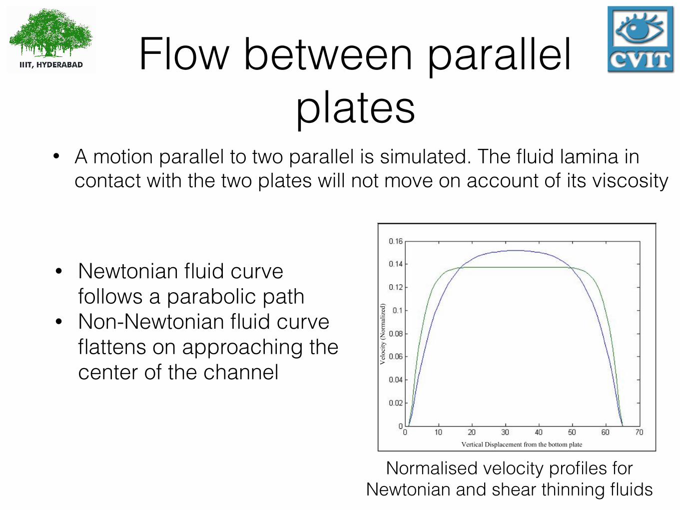
• A motion parallel to two parallel is simulated. The fluid lamina in contact with the two plates will not move on account of its viscosity

• Newtonian fluid curve follows a parabolic path

• Non-Newtonian fluid curve flattens on approaching the center of the channel

Normalised velocity profiles for Newtonian and shear thinning fluids

Conclusions & Future Work

• Simulated both Newtonian and non-Newtonian fluids accurately at upto 600 MLUPS using a single GPU and 900 MLUPS using two GPUs

• We have dealt with laminar flows in this work. A study on turbulent fluids using LBM is an interesting area for future work.

• Visual quality of the simulations can be enhanced using ray-tracing.

• Building upon our work to simulate out of core grids (5123 and above) is another interesting area for future work.

Thank You!

Interactive Simulation of Generalised Newtonian …somay/LBM/LBM_presentation.pdfInteractive...

Documents

Transcript of Interactive Simulation of Generalised Newtonian …somay/LBM/LBM_presentation.pdfInteractive...