Interactive Image Matting for Multiple Layers

Dheeraj Singaraju Rene VidalCenter for Imaging Science, Johns Hopkins University, Baltimore, MD 21218, USA

AbstractImage matting deals with finding the probability that

each pixel in an image belongs to a user specified ‘object’or to the remaining ‘background’. Most existing methodsestimate the mattes for two groups only. Moreover, mostof these methods estimate the mattes with a particular biastowards the object and hence the resulting mattes do notsum up to 1 across the different groups. In this work, wepropose a general framework to estimate the alpha mattesfor multiple image layers. The mattes are estimated as thesolution to the Dirichlet problem on a combinatorial graphwith boundary conditions. We consider the constrained op-timization problem that enforces the alpha mattes to takevalues in [0, 1] and sum up to 1 at each pixel. We also an-alyze the properties of the solution obtained by relaxing ei-ther of the two constraints. Experiments demonstrate thatour proposed method can be used to extract accurate mat-tes of multiple objects with little user interaction.

1. IntroductionImage matting refers to the problem of assigning to each

pixel in an image, a probabilistic measure of whether it be-longs to a desired object or not. This problem finds numer-ous applications in image editing, where the user is inter-ested only in the pixels corresponding to a particular object,rather than in the whole image. In such cases, one prefersassigning soft values to the pixels rather than a hard classifi-cation. This is because there can be ambiguous areas whereone cannot make clear cut decisions about the pixels’ mem-bership. Matting therefore deals with assigning a partialopacity value α ∈ [0, 1] to each pixel, such that pixels thatdefinitely belong to the object or background are assigned avalue α = 1 or α = 0 respectively. More specifically, thematting problem tries to estimate the value αi at each pixeli, such that its intensity Ii can be expressed in terms of thetrue foreground and background intensities Fi and Bi as

Ii = αiFi + (1− αi)Bi. (1)

Note that in (1), the number of unknowns is more thanthe number of independent equations, thereby making thematting problem ill posed. Therefore, matting algorithmstypically require some user interaction that specifies theobject of interest and the background, thereby embedding

Figure 1. Typical example of the image matting problem. Left:Given image with a toy object. Right: Desired matte of the toy.

some constraints in the image. User interaction is providedin the form of a trimap that specifies the regions that defi-nitely belong to the object and the background, and an inter-mediate region where the mattes need to be estimated. Earlymethods use the trimap to learn intensity models for the ob-ject as well as the background [2, 11, 3]. These learnedintensity models are subsequently used to predict the alphamattes in the intermediate region. Also, Sun et al. [12] usethe image gradients to estimate the mattes as the solution tothe Dirichlet problem with boundary conditions.

A common criticism of these methods is that they typ-ically require an accurate trimap with a fairly narrow in-termediate region to produce good results. Moreover, theygive erroneous results if the background and object havesimilar intensity distributions or if the image intensities donot vary smoothly in the intermediate region. These issueshave motivated the development of methods that extract themattes for images with complex intensity variations. Oneline of work employs popular segmentation techniques forthe problem of image matting [10, 5, 1]. However, thesemethods enforce the regions in the image to be connected.This is a major limitation, as these methods cannot deal withimages such as Figure 1, where the actual matte has holes.

More recent work addresses the aforementioned issuesand lets the user extract accurate mattes for challenging im-ages with low levels of interaction [14, 8, 6, 16, 15, 13].However, a fundamental limitation of these methods is thatthey extract mattes for two groups only. The only existingwork dealing with multiple groups is the Spectral Mattingalgorithm proposed by Levin et al. [9]. They propose to usethe eigenvectors of the so-called Matting Laplacian matrixto obtain the mattes for several layers. In reality, the algo-rithm uses multiple eigenvectors to estimate the matte for asingle object. Moreover, the experiments are restricted toextracting the mattes for two layers only.

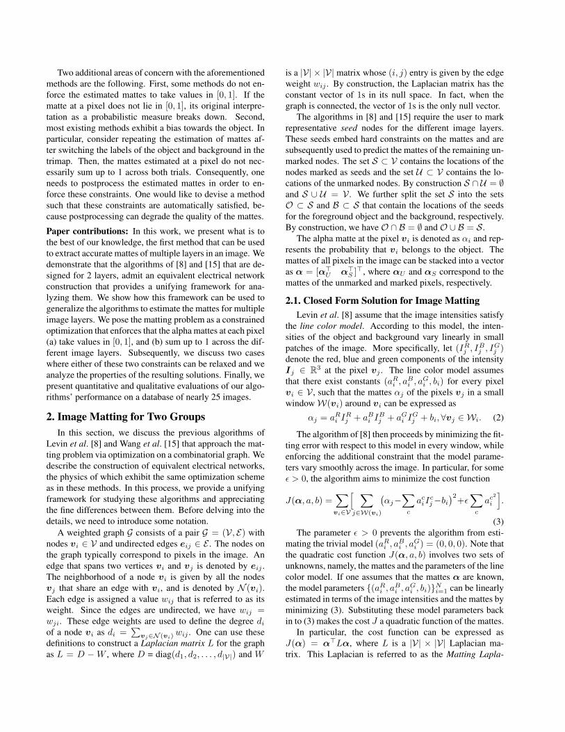
Two additional areas of concern with the aforementionedmethods are the following. First, some methods do not en-force the estimated mattes to take values in [0, 1]. If thematte at a pixel does not lie in [0, 1], its original interpre-tation as a probabilistic measure breaks down. Second,most existing methods exhibit a bias towards the object. Inparticular, consider repeating the estimation of mattes af-ter switching the labels of the object and background in thetrimap. Then, the mattes estimated at a pixel do not nec-essarily sum up to 1 across both trials. Consequently, oneneeds to postprocess the estimated mattes in order to en-force these constraints. One would like to devise a methodsuch that these constraints are automatically satisfied, be-cause postprocessing can degrade the quality of the mattes.

Paper contributions: In this work, we present what is tothe best of our knowledge, the first method that can be usedto extract accurate mattes of multiple layers in an image. Wedemonstrate that the algorithms of [8] and [15] that are de-signed for 2 layers, admit an equivalent electrical networkconstruction that provides a unifying framework for ana-lyzing them. We show how this framework can be used togeneralize the algorithms to estimate the mattes for multipleimage layers. We pose the matting problem as a constrainedoptimization that enforces that the alpha mattes at each pixel(a) take values in [0, 1], and (b) sum up to 1 across the dif-ferent image layers. Subsequently, we discuss two caseswhere either of these two constraints can be relaxed and weanalyze the properties of the resulting solutions. Finally, wepresent quantitative and qualitative evaluations of our algo-rithms’ performance on a database of nearly 25 images.

2. Image Matting for Two GroupsIn this section, we discuss the previous algorithms of

Levin et al. [8] and Wang et al. [15] that approach the mat-ting problem via optimization on a combinatorial graph. Wedescribe the construction of equivalent electrical networks,the physics of which exhibit the same optimization schemeas in these methods. In this process, we provide a unifyingframework for studying these algorithms and appreciatingthe fine differences between them. Before delving into thedetails, we need to introduce some notation.

A weighted graph G consists of a pair G = (V, E) withnodes vi ∈ V and undirected edges eij ∈ E . The nodes onthe graph typically correspond to pixels in the image. Anedge that spans two vertices vi and vj is denoted by eij .The neighborhood of a node vi is given by all the nodesvj that share an edge with vi, and is denoted by N (vi).Each edge is assigned a value wij that is referred to as itsweight. Since the edges are undirected, we have wij =wji. These edge weights are used to define the degree diof a node vi as di =

∑vj∈N (vi)

wij . One can use thesedefinitions to construct a Laplacian matrix L for the graphas L = D −W , where D = diag(d1, d2, . . . , d|V|) and W

is a |V| × |V| matrix whose (i, j) entry is given by the edgeweight wij . By construction, the Laplacian matrix has theconstant vector of 1s in its null space. In fact, when thegraph is connected, the vector of 1s is the only null vector.

The algorithms in [8] and [15] require the user to markrepresentative seed nodes for the different image layers.These seeds embed hard constraints on the mattes and aresubsequently used to predict the mattes of the remaining un-marked nodes. The set S ⊂ V contains the locations of thenodes marked as seeds and the set U ⊂ V contains the lo-cations of the unmarked nodes. By construction S ∩ U = ∅and S ∪ U = V . We further split the set S into the setsO ⊂ S and B ⊂ S that contain the locations of the seedsfor the foreground object and the background, respectively.By construction, we have O ∩ B = ∅ and O ∪ B = S.

The alpha matte at the pixel vi is denoted as αi and rep-resents the probability that vi belongs to the object. Themattes of all pixels in the image can be stacked into a vectoras α = [α>U α>S ]>, where αU and αS correspond to themattes of the unmarked and marked pixels, respectively.

2.1. Closed Form Solution for Image MattingLevin et al. [8] assume that the image intensities satisfy

the line color model. According to this model, the inten-sities of the object and background vary linearly in smallpatches of the image. More specifically, let (IRj , I

Bj , I

Gj )

denote the red, blue and green components of the intensityIj ∈ R3 at the pixel vj . The line color model assumesthat there exist constants (aRi , a

Bi , a

Gi , bi) for every pixel

vi ∈ V , such that the mattes αj of the pixels vj in a smallwindowW(vi) around vi can be expressed as

αj = aRi IRj + aBi I

Bj + aGi I

Gj + bi,∀vj ∈ Wi. (2)

The algorithm of [8] then proceeds by minimizing the fit-ting error with respect to this model in every window, whileenforcing the additional constraint that the model parame-ters vary smoothly across the image. In particular, for someε > 0, the algorithm aims to minimize the cost function

J(α, a, b) =∑vi∈V

[ ∑j∈W(vi)

(αj−

∑c

aciIcj−bi

)2+ε∑c

ac2

i

].

(3)The parameter ε > 0 prevents the algorithm from esti-

mating the trivial model (aRi , aBi , a

Gi ) = (0, 0, 0). Note that

the quadratic cost function J(α, a, b) involves two sets ofunknowns, namely, the mattes and the parameters of the linecolor model. If one assumes that the mattes α are known,the model parameters {(aRi , aBi , aGi , bi)}Ni=1 can be linearlyestimated in terms of the image intensities and the mattes byminimizing (3). Substituting these model parameters backin to (3) makes the cost J a quadratic function of the mattes.

In particular, the cost function can be expressed asJ(α) = α>Lα, where L is a |V| × |V| Laplacian ma-trix. This Laplacian is referred to as the Matting Lapla-

cian and essentially captures the local statistics of the in-tensity variations in a small window around each pixel [8].We shall now introduce some terms needed for defining theMatting Laplacian. Consider a window W(vk) around apixel vk ∈ V and let the number of pixels in this win-dow be nk. Let the mean and the covariance of the inten-sities of the pixels in W(vk) be denoted as µk ∈ R3 andΣk ∈ R3×3. Denoting an m×m identity matrix as Im, [8]showed that the Matting Laplacian can be constructed fromthe edge weights wij that are defined as∑k|vi,vj∈W(vk)

n−1k

(1+(Ii−µk)>(Σk+

ε

nkI3)−1(Ij−µk)

). (4)

Note that these weights can be positive or negative. Theneighborhood structure however ensures that the graph isconnected. Recall that the user marks some pixels in theimage as seeds that are representative of the object and thebackground. To this effect, we define a vector s ∈ R|S|,such that an entry of s is set to 1 or 0 depending on whetherit corresponds to the seed of an object or background, re-spectively. Also, for some λ > 0, we define a matrixΛ =λI|S|. The mattes in the image are then estimated as

α = argminα

[ ∑eij∈E

wij(αi − αj)2 +∑i∈S

λ(αi − si)2

]

= argminα

[α>Lα+ λ(αS − s)>(αS − s)

](5)

= argminα

[α>U α>S s>

]LU B> 0B LS + Λ −Λ0 −Λ Λ

αUαSs

.Noticing that the expression in (3) is non-negative, [8]

showed that the Matting Laplacian is positive semi-definite.This makes the cost function in (5) convex and thereforethe optimization has a unique minimizer that can be linearlyestimated in closed form as

αS = [A+ Λ]−1Λs, and

αU = −L−1U B>αS = −L−1

U B>[A+ Λ]−1Λs,(6)

where A = LS −BL−1U B>. The algorithm of Levin et al.

[8] employs the above optimization by choosing a large fi-nite valued λ, while the algorithm of Wang et al. [15] worksin the limiting case by choosing λ = ∞. We note that [15]employs a modification of the Matting Laplacian. However,it suffices for the purpose of our analysis that the modifiedmatrix is also a positive semi-definite Laplacian matrix.

2.2. Electrical Networks for Image Matting

It is interesting to note that there exists an equivalentelectrical network that solves the optimization problem in(5). In particular, one constructs a network as shown in Fig-ure 2, such that each node in the graph associated with theimage is equivalent to a node on the network.

O

O

B

Bwij

ji ji

Figure 2. Equivalent construction of combinatorial graphs andelectrical networks.

The edge weights correspond to the conductance val-ues of resistors connected between neighboring nodes, i.e.

1Rij

= wij . Since the edge weights wij are not all pos-itive, one can argue that this system might not be phys-ically realizable. However, we note that the network isconstrained to dissipate positive energy due to the positivesemi-definiteness of the Laplacian. Therefore, we can thinkof the image as a real resistive load that dissipates energy.The seeded nodes are connected to the network ground andunit voltage sources by resistive impedances of value 1

λ .In particular, the background seeds are connected to theground and the object seeds are connected to the unit volt-age sources. Hence, we have s = 1V at the voltage sourcesand s = 0V at the ground, where all measurements are withrespect to the network’s ground.

From network theory, we know that the potentials x atthe nodes in the network distribute themselves such thatthey minimize the energy dissipated by the network. Thepotentials can therefore be estimated as

x = argminx

[ ∑eij∈E

1Rij

(xi−xj)2+∑i∈S

λ(xi−si)2

]. (7)

We note that this is exactly the same expression as in (5).Therefore, if one were to construct the equivalent networkand measure the potentials at the nodes they would give usthe required alpha mattes.

In what follows, we shall show that as λ → ∞, thefraction (η) of work done by the electrical sources that isused to drive the load is maximized. Note that one canuse the positive definiteness of L and the connectednessof the graph to show that the matrix A is positive definite.Now, consider the singular value decomposition of the ma-trix A. We have A = UΣAU>, where U = [u1 . . . u|S|]and ΣA = diag(σ1, . . . , σ|S|), σ1 ≥ σ2 ≥ · · · ≥ σ|S| > 0.We can then explicitly evaluate η as

η =Eload

Etotal=

x>Lx

x>Lx+ (xS − s)>Λ(xS − s)(8)

=(s>Λ)

([A+ Λ]−1A[A+ Λ]−1

)(Λs)

(s>Λ)(

Λ−1 − [A+ Λ]−1)

(Λs)=

|S|∑i=1

σi(u>i s)2

(σi

λ + 1)2

|S|∑i=1

σi(u>i s)2

(σi

λ + 1)

.

Since λ > 0 and ∀i = 1, . . . , |S|, σi > 0, we have that1 + σi

λ > 1. Given this observation, it can be verified that∀λ ∈ (0,∞), η < 1 and lim

λ→∞η = 1. The fractional en-

ergy delivered to the load is therefore maximized by settingλ = ∞. In the network, this limiting case corresponds tosetting the values of impedances between the sources andthe load to zero. In terms of the image, this forces the mat-tes at the pixels marked by the scribbles to be 1 for the fore-ground object and 0 for the background.

The algorithm of [8] solves the optimization problem in(5) by setting λ to be a large finite valued number. Sincethere is always a finite potential drop across the resistorsconnecting the voltage source and the grounds to the image,we note that the mattes (potentials) at the seeds are closeto the desired values but not equal. The algorithm of Wanget al. [15] corresponds to the limiting case of λ = ∞ andforces the mattes at the seeds to be equal to the desired val-ues. The numerical framework of the latter is referred toas the solution to the combinatorial Dirichlet problem withboundary conditions. Based on the argument given above,we favor the optimization of [15] over that of [8] becauseit helps in utilizing the scribbles to the maximum extent toprovide knowledge about the unknown mattes.

3. Image Matting for Multiple GroupsIn this section, we show how to solve the matting prob-

lem for n ≥ 2 image layers, by using generalizations ofthe methods discussed in Section 2. Essentially, we assumethat the intensity of each pixel in the query image can be ex-pressed as the convex linear combination of the intensitiesat the same pixel location in the n image layers. We are theninterested in estimating partial opacity values at each pixelas the probability of belonging to one of the image layers.

In what follows, we denote the intensity of a pixel vi ∈V in the query image by Ii. Similarly, the intensity of a pixelvi ∈ V in the jth image layer is denoted by F ji , where 1 ≤j ≤ n. The alpha matte at a pixel vi ∈ V with respect to thejth image layer is denoted by αji . Given these definitions,the matting problem requires us to estimate alpha mattes{αji}nj=1 and the intensities {F ji }nj=1 of the n image layersat each pixel vi ∈ V , such that we have

Ii=n∑j=1

αjiFji , s.t.

n∑j=1

αji =1, and {αji}nj=1 ∈ [0, 1]. (9)

We shall pose this matting problem as an optimizationproblem on combinatorial graphs. While we retain mostof the notations from Section 2, we need to introduce newnotation for the sets that contain the seeds’ locations. Inparticular, we split the set S that contains the locations of allthe seeds into the sets R1,R2, . . . ,Rn, where Ri containsthe seed locations for the ith layer. By construction, we have∪ni=1Ri = S and ∀1 ≤ i < j ≤ n,Ri ∩Rj = ∅.

Algorithm 1 (Image matting for n ≥ 2 image layers)1: Given an image, construct the matting Laplacian L forthe image as described in Section 2.2: For each image layer j ∈ {1, · · · , n}, fix the mattes atthe seeds as αji = 1 if vi ∈ Rj and αji = 0 if vi ∈ S \Rj .3: Estimate the alpha mattes {αjU}nj=1 for the unmarkedpixels with respect to the n image layers as

{αjU}nj=1 =argmin

{αjU}n

j=1

n∑j=1

[αj>Lαj

](10)

such that (a) ∀j ∈ {1, . . . , n},0 ≤ αjU ≤ 1, and

(b)n∑j=1

αjU = 1. (11)

We propose to solve this problem by minimizing the sumof the cost functions associated with the estimation of mat-tes for each image layer. Unlike [8] and [15], we proposeto impose constraints that the mattes sum up to 1 at eachpixel, and take values in [0, 1]. In particular, we proposethat the matting problem can be solved using Algorithm 1.Notice that this is a standard optimization of minimizing aquadratic function subject to linear constraints. Recall fromSection 2 that the cost function in (10), is a convex func-tion of the alpha mattes. Also, notice that the set of feasiblesolutions of the mattes {αjU}nj=1 is compact and convex.Therefore, the optimization problem posed in Algorithm 1is guaranteed to have a unique solution. However, this op-timization can be computationally cumbersome due to thelarge number of unknown variables. In what follows, weshall discuss relaxing either one of the constraints and ana-lyze its effect on the solution to the optimization problem.

3.1. Image matting for multiple layers, without con-straining the sum of the mattes at a pixel

We analyze the properties of the mattes obtained by solv-ing the optimization problem of (10) without enforcing themattes to take values between 0 and 1. In particular, Theo-rem 1 states an important consequence of this case.

Theorem 1 The alpha mattes obtained as the solution toAlgorithm 1 without imposing the constraint that they takevalues between 0 and 1, are naturally constrained to sumup to 1 at every pixel.

Proof. Notice that the set of feasible solutions for the mattesis convex, even when we do not impose constraint (a). Theoptimization problem is hence guaranteed to have a uniquesolution. Now, we know that this solution must satisfy theKarusch-Kuhn-Tucker (KKT) conditions [7]. In particular,the KKT conditions guarantee the existence of a vector Γ ∈R|U| such that the solution αU satisfies

∀j ∈ {1, . . . , n}, LUαjU +B>αjS + Γ = 0. (12)

The entries of Γ are the Lagrange multipliers for the con-straints that the mattes sum up to one at each pixel. We nowassume that the mattes sum up to one, and show that Γ=0.This is equivalent to proving that the constraint (b) in (11) isautomatically satisfied without explicitly enforcing it. As-sume that

∑nj=1α

jU = 1. Also, recall that by construction,∑n

j=1αjS = 1. Now summing up the KKT conditions in

(12) across all the image layers gives us

n∑j=1

[LUαjU +B>αjS + Γ] = LU1+B>1+nΓ = 0 (13)

Recall that the vector of 1s lies in the null space of L,and hence we have LU1 + B>1 = 0 Therefore, we canconclude from (13) that Γ = 0. This implies that the so-lution automatically satisfies the constraint that the mattessum up to 1 at each unmarked pixel. In fact, if one does notenforce constraint (a) in (11), then the solution is the same,irrespective of whether constraint (b) is enforced or not.

This is an important result which follows intuitively fromthe well known Superposition Theorem in electrical net-work theory [4]. It is important to notice that the estima-tion of mattes for the ith image layer is posed as the solutionto the Dirichlet problem with boundary conditions. In fact,this is a simple extension of [15], where the ith image layeris treated as the foreground and the rest of the layers aretreated as the background. Theorem 1 guarantees that theestimation of the mattes for any n− 1 of the n image layersautomatically determines the mattes for the remaining layer.

Wang et al. [15] claim that this optimization schemefinds analogies in the theory of random walks. Therefore,a standard result states that the mattes are constrained to liebetween 0 and 1. However, this result is derived specifi-cally for graphs with positive edge weights. This is not truefor the graphs constructed for the matting problem since thegraphs’ edge weights are both positive and negative.

In fact, Figure 3 gives an example where the system hasa positive semi-definite Laplacian matrix, but the obtainedpotentials (mattes) do not all lie in [0, 1]. Note that xc takesthe value 4

3 on switching the locations of the voltage sourceand the ground. An easy fix employed by [8] and [15] to re-solve this issue, is to clip all the alpha values such that theytake values in [0, 1]. This scheme might give results that arevisually pleasing, but they might not obey the KKT con-ditions. Moreover, the postprocessed mattes at each pixelmight not sum up to 1 across all the layers anymore.

3.2. Image matting for multiple layers, without con-straining the limits of the mattes

In this section, we discuss the properties of the solutionof Algorithm 1, when we do not enforce the constraint thatthe mattes sum up to 1 at each pixel. Before we discuss

the general scheme for n ≥ 2 layers, we consider the sim-ple case of estimating the mattes for n = 2 layers. In thiscase, the mattes at the unmarked pixels are estimated as thesolution of the quadratic programming problem given by

αjU = argminαj

U

[αjU>LUα

jU + 2αjU

>BαS +α>SLSαS

],

subject to 0 ≤ αjU ≤ 1, for j = 1, 2. (14)

Note that the set of feasible solutions for the mattes ofthe unmarked pixels is given by [0, 1]|U|, which is a compactconvex set. Also, the objective function being minimized in(14) is a convex function of the alpha mattes. Hence, theoptimization problem is guaranteed to have a unique mini-mizer. In this case, the KKT conditions guarantee the exis-tence of |U|×|U| diagonal matrices {Λj0}2j=1 and {Λj1}2j=1,with non-positive entries such that the solution αjU for thejth image layer satisfies

LUαU +B>αS + Λ0 − Λ1 = 0, and

Λj0αjU = 0,Λji (1−α

jU ) = 0, j = 1, 2.

(15)

In what follows, we denote the (i, i) diagonal entry of{Λjk}

j=1,2k=0,1 as λjki ≤ 0. Notice that if the matte αji at the

ith unmarked pixel with respect to the jth image layer liesbetween 0 and 1, then the KKT conditions state that the as-sociated slack variables λj0i and λj1i are equal to zero. Con-sequently, the ith row of the first equation in (15) gives us

the result that αji =P

vk∈N(vk) wikαjkP

vk∈N(vi)wik

. In particular, this

implies that αi can be expressed as the weighted average ofthe mattes of the neighboring pixels. But, when αji = 0 orαji = 1, we see that αji is not the weighted average of themattes at the neighboring pixels and this is accounted for bythe slack variables λj0i and λj1i. Recall from Section 3.1 thatthe methods of [8] and [15] clip the estimated mattes to takevalues between 0 and 1, when necessary. This step is some-what equivalent to using such slack variables. However, onealso needs to re-adjust the alpha mattes at the unmarked pix-els that lie in the neighborhoods of the pixels whose mattesare clipped. In particular, they need to be adjusted so thatthey still satisfy the KKT conditions. However, this step isneglected in the methods of [8] and [15].

L =

0.75 −1 0.25−1 2 −10.25 −1 0.75

Figure 3. Example where all the potentials do not lie in [0, 1].

We now consider the problem of solving this constrainedoptimization for n ≥ 2 image layers. In particular, we wantto analyze whether the sum of the mattes at each pixel isconstrained to be 1 or not. Theorem 2 states an importantproperty of this optimization that the sum of mattes is en-forced to be 1, only when n = 2 and not otherwise.

Theorem 2 The alpha mattes obtained as the solution toAlgorithm 1 without imposing the constraint that they sumup to 1 at each pixel, are in fact naturally constrained tosum up to 1 at each pixel when n = 2, but not when n > 2.

Proof. Consider the following optimization problem for es-timating the mattes at the unmarked nodes.

{αjU}nj=1 = argmin

{αjU}n

j=1

n∑j=1

[αjU>LUα

jU + 2αjU

>BαjS

],

s.t. 0 ≤ {αjU}nj=1 ≤ 1, and

n∑j=1

αjU = 1. (16)

As discussed earlier, the KKT conditions guarantee theexistence of diagonal matrices {Λj0}ni=1 and {Λj1}ni=1, anda vector Γ, such that the solution {αjU}nj=1 satisfies

∀1 ≤ j ≤ n,LUαjU +B>αjS + Λj0 − Λj1 + Γ = 0, and

∀1 ≤ j ≤ n,Λj0αju = 0,Λji (1−αjU ) = 0. (17)

Γ acts as a Lagrange multiplier for the constraint that themattes sum up to 1. We now assume that the mattes sumup to 1 at each pixel and inspect the value of Γ. Essentially,if Γ = 0, it means that the estimated mattes are naturallyconstrained to sum up to 1 at each pixel. Assuming that themattes sum up to 1, we sum up the first expression in (17)across all the image layers to conclude that

n∑j=1

Λj0 −n∑j=1

Λj1 + nΓ = 0 (18)

This relationship is derived using the fact that LU1 +B>1 = 0. We now inspect the mattes at a pixel vi ∈ Uand analyze all the possible solutions. Firstly, consider thecase when the mattes {αji}kj=1 of the first k < n− 1 imagelayers are identically equal to 0 and the remaining mattes{αji}nj=k+1 take values in (0, 1). We can always considersuch reordering of the image layers without any loss of gen-erality. We see that the variables {λj1i}nj=1 and {λj0i}nj=k+1

are equal to zero. Substituting these values in (18), givesγi +

∑kj=1 λ

j0i = 0. Therefore, γi is non-negative, and

is equal to zero if and only if the variables {λj0i}kj=1 areidentically equal to zero. Since these variables are not con-strained to be zero valued, we see that γi is not equal tozero. It is precisely due to this case exactly that the mattesare not constrained to sum up to 1, when n > 2.

However, this case cannot arise when n = 2. In factfor n = 2, we see that both the mattes take values ineither (0, 1) or in {0, 1}. In the first case, we see thatλ1

0i = λ20i = λ1

1i = λ11i = 0. For the second case, as-

sume without loss of generality that α1i = 0 and α2

i = 1.We then have λ1

1i = λ20i = 0. Moreover, we notice that set-

ting λ10i = λ2

1i satisfies the KKT conditions. Hence, we canconclude that γi = 0 in both cases. Consequently, the mat-tes are naturally constrained to sum up to 1 at each pixel,for n = 2.

4. Experiments

We denote the variants of Algorithm 1 discussed in Sec-tions 3.1 and 3.2 as Algorithm 1a and Algorithm 1b respec-tively. We now evaluate these algorithms’ performance onthe database proposed by Levin et al. [9]. The databaseconsists of images of three different toys, namely a lion, amonkey and a monster. Each toy is imaged against 8 differ-ent backgrounds and so the database has 24 distinct images.The database provides the ground truth mattes for the toys.All the images are of size 560× 820 and are normalized totake values between 0 and 1. In our experiments, the Mat-ting Laplacian for each image is estimated as described inSection 2.1, using windows of size 3×3 and with ε = 10−6.

4.1. Quantitative Evaluation for n = 2 LayersWe present a quantitative evaluation of our algorithms

on the described database. We follow the same procedureas in [9] and define the trimap by considering the pixelswhose true mattes lie between 0.05 and 0.95 and dilatingthis region by 4 pixels. The algorithms performance is thenevaluated by considering the SSD (sum of squared differ-ences) error between the estimated mattes and the groundtruth. Table 1 shows the statistics of performance.

We see that the performance of both variants is on par.Recall that the numerical framework of Algorithm 1a is verysimilar to that of the closed form matting solution proposedby Levin et al. [8]. Consequently, both these algorithmswould have similar performances. The analysis in [9] showsthat the algorithm of [8] performs better than the mattingalgorithms of [12, 5, 14] and is outperformed only by theSpectral Matting algorithm. Therefore, we conclude thatboth variants of Algorithm 1 potentially match up to thestate of the art algorithms.

Algorithm 1aToy Mean MedianLion 532.06 486.24Monkey 273.34 277.03Monster 822.07 958.06

Algorithm 1bToy Mean MedianLion 547.00 509.18Monkey 273.40 278.00Monster 796.03 864.42

Table 1. Statistics of SSD errors in estimating mattes of 2 layers.

4.2. Qualitative Evaluation for n ≥ 2 LayersWe now present results of using Algorithm 1a to extract

mattes for n > 2 image layers with low levels of user in-teraction. Since there is no ground truth data available formultiple layers, we validate the performance visually. Inparticular, we first estimate the matte for the multiple layersusing Algorithm 1a. We then use the scheme outlined in [8]to reconstruct the intensities of each image layer. Finally,we show the contribution of each image layer to the queryimage. Figures 4 and 5 show the results for the extraction ofmattes for 3 and 5 image layers, respectively. The scribblesare color coded to demarcate between the different imagelayers. We note that the results visually appear to be quitegood. The results highlight a disadvantage of our methodthat the mattes can be erroneous if the intensities near theboundary of adjoining image layers are similar. This prob-lem can be fixed by adding more seeds, and hence at anexpense of increased levels of user interaction.

5. ConclusionsWe have proposed a constrained optimization problem

to extract accurate mattes for multiple image layers withlow levels of user interaction. We discussed two variants ofthe method where we relaxed the constraints of the prob-lem and presented a theoretical analysis of the properties ofthe estimated mattes. Experimental evaluation of both thesevariants shows that they provide visually pleasing results.

Acknowledgments. Work supported by JHU startup funds,by grants NSF CAREER ISS-0447739, NSF EHS-0509101,and ONR N00014-05-1083, and by contract APL-934652.

References[1] X. Bai and G. Sapiro. A Geodesic Framework for Fast Interactive

Image and Video Segmentation and Matting. In ICCV, pages 1–8,2007.

[2] A. Berman, A. Dadourian, and P. Vlahos. Method for Removingfrom an Image the Background Surrounding a Selected Object. USPatent no. 6,134,346, October 2000.

(a) Scribbles for marking seeds (b) αmonsterFmonster

(c) αskyFsky (d) αwaterFwater

Figure 4. Extracting 3 image layers using Algorithm 1a.

[3] Y.-Y. Chuang, B. Curless, D. Salesin, and R. Szeliski. A BayesianApproach to Digital Matting. In CVPR (2), pages 264–271, 2001.

[4] P. Doyle and L. Snell. Random walks and electric networks. Num-ber 22 in The Carus Mathematical Monographs. The MathematicalSociety of America, 1984.

[5] L. Grady, T. Schiwietz, S. Aharon, and R. Westermann. RandomWalks for Interactive Alpha-Matting. In ICVIIP, pages 423–429,September 2005.

[6] Y. Guan, W. Chen, X. Liang, Z. Ding, and Q. Peng. Easy Matting:A Stroke Based Approach for Continuous Image Matting. In Euro-graphics 2006, volume 25, pages 567–576, 2006.

[7] H. W. Kuhn and A. W. Tucker. Nonlinear Programming. In 2ndBerkeley Symposium, pages 481–492, 1951.

[8] A. Levin, D. Lischinski, and Y. Weiss. A Closed Form Solution toNatural Image Matting. IEEE Trans. on PAMI, 30(2): 228–242, 2008

[9] A. Levin, A. Rav-Acha, and D. Lischinski. Spectral Matting. InCVPR, Pages 1–8, 2007.

[10] C. Rother, V. Kolmogorov, and A. Blake. ”Grabcut”: InteractiveForeground Extraction Using Iterated Graph Cuts. ACM Trans.Graph., 23(3):309–314, 2004.

[11] M. A. Ruzon and C. Tomasi. Alpha Estimation in Natural Images.In CVPR, pages 1018–1025, 2000.

[12] J. Sun, J. Jia, C.-K. Tang, and H.-Y. Shum. Poisson Matting. ACMTrans. Graph., 23(3):315–321, 2004.

[13] J. Wang, M. Agrawala, and M. F. Cohen. Soft Scissors: An Interac-tive Tool for Realtime High Quality Matting. ACM Trans. Graph.,26(3):9, 2007.

[14] J. Wang and M. F. Cohen. An Iterative Optimization Approach forUnified Image Segmentation and Matting. In ICCV, pages 936–943,2005.

[15] J. Wang and M. F. Cohen. Optimized Color Sampling for RobustMatting. In CVPR, Pages 1–8, 2007.

[16] J. Wang and M. F. Cohen. Simultaneous Matting and Compositing.In CVPR, Pages 1–8, 2007.

(a) Scribbles for marking seeds (b) αlionFlion

(c) αskyFsky (d) αhillFhill

(e) αsandFsand (f) αwaterFwater

Figure 5. Extracting 5 image layers using Algorithm 1a.