InteractiveGraph Analyticswith SparkA talk by Daniel Darabos about the design and implementation of the LynxKite analytics application

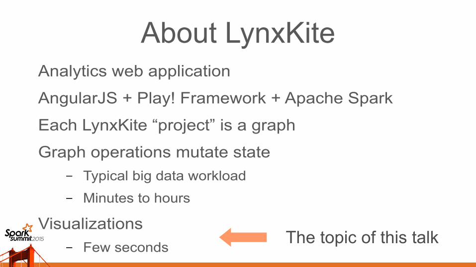
About LynxKiteAnalytics web application

AngularJS + Play! Framework + Apache Spark

Each LynxKite “project” is a graph

Graph operations mutate state– Typical big data workload

– Minutes to hours

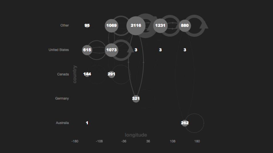
Visualizations– Few seconds

The topic of this talk

Idea 1:

Avoid processing unused attributes

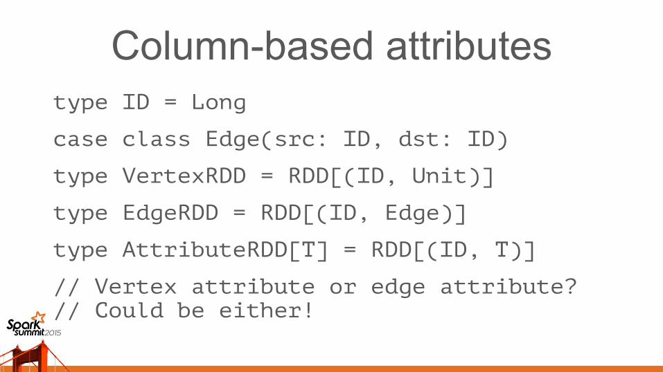
Column-based attributestype ID = Long

case class Edge(src: ID, dst: ID)

type VertexRDD = RDD[(ID, Unit)]

type EdgeRDD = RDD[(ID, Edge)]

type AttributeRDD[T] = RDD[(ID, T)]

// Vertex attribute or edge attribute?// Could be either!

Column-based attributesCan process just the attributes we need

Easy to add an attribute

Simple and flexible– Edges between vertices of two different graphs

– Edges between edges of two different graphs

A lot of joining

Idea 2:

Make joins fast

Co-located loadingJoin is faster for co-partitioned RDDs

– Spark only has to fetch one partition

Even faster for co-located RDDs– The partition is already in the right place

When loading attributes we make a seemingly useless join that causes two RDDs to be co-located

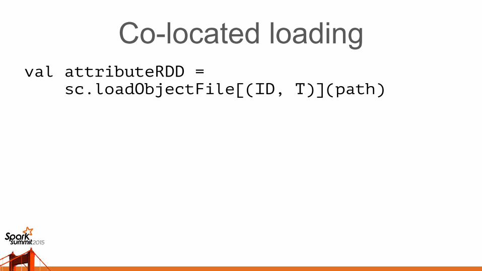
Co-located loadingval attributeRDD = sc.loadObjectFile[(ID, T)](path)

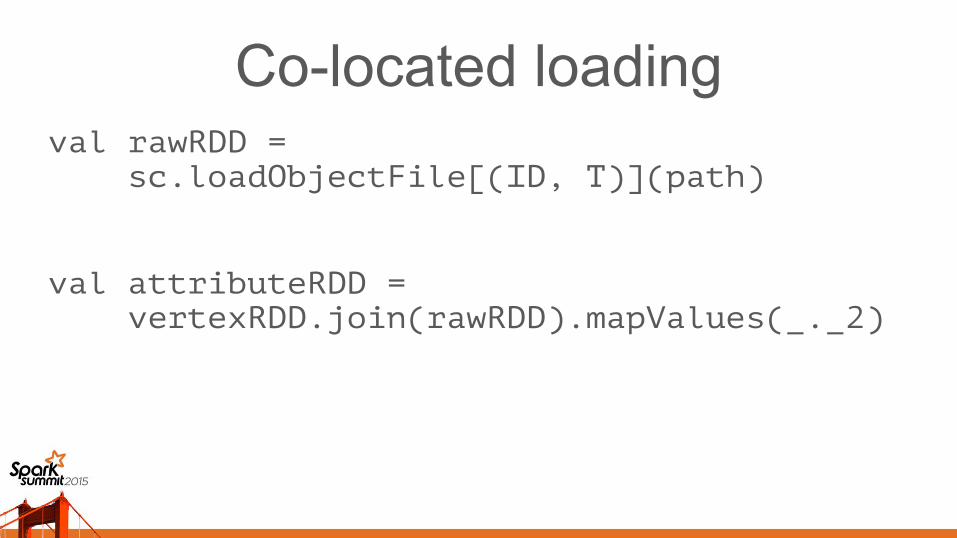
Co-located loadingval rawRDD = sc.loadObjectFile[(ID, T)](path)

val attributeRDD = vertexRDD.join(rawRDD).mapValues(_._2)

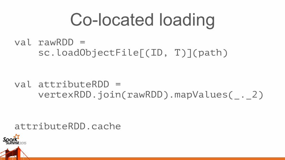
Co-located loadingval rawRDD = sc.loadObjectFile[(ID, T)](path)

val attributeRDD = vertexRDD.join(rawRDD).mapValues(_._2)

attributeRDD.cache

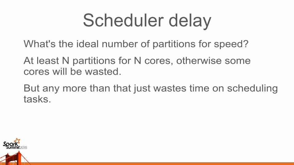
Scheduler delayWhat's the ideal number of partitions for speed?

At least N partitions for N cores, otherwise some cores will be wasted.

But any more than that just wastes time on scheduling tasks.

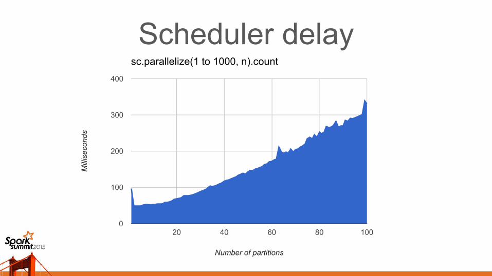
sc.parallelize(1 to 1000, n).count

20 40 60 80 1000

100

200

300

400

Number of partitions

Mill

isec

onds

Scheduler delay

GC pausesCan be tens of seconds on high-memory machines

Bad for interactive experience

Need to avoid creating big objects

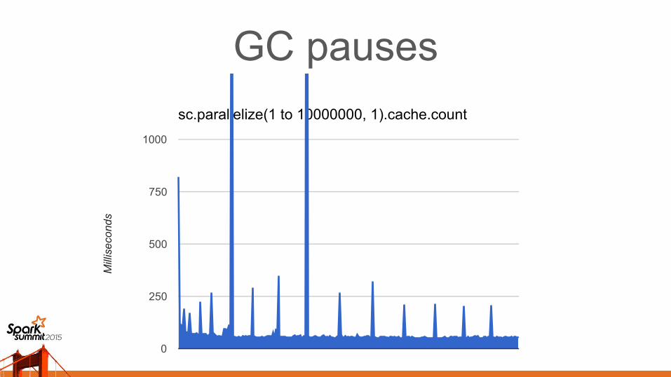
GC pauses

sc.parallelize(1 to 10000000, 1).cache.count

0

250

500

750

1000

Mill

ise

cond

s

Sorted RDDsSpeeds up the last step of the join

The insides of the partitions are kept sorted

Merging sorted sequences is fast

Doesn't require building a large hashmap

10 × speedup + GC benefit– 2 × if cost of sorting is included

– sorting cost is amortized across many joins

Benefits other operations too (e.g. distinct)

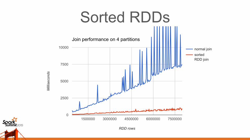
Sorted RDDsJoin performance on 4 partitions

normal join

sortedRDD join

1500000 3000000 4500000 6000000 75000000

2500

5000

7500

10000

RDD rows

Mill

ise

cond

s

Idea 3:

Do not read/compute all the data

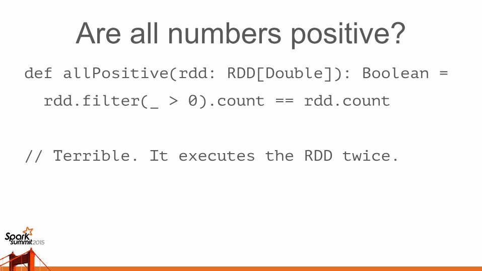
Are all numbers positive?def allPositive(rdd: RDD[Double]): Boolean =

rdd.filter(_ > 0).count == rdd.count

// Terrible. It executes the RDD twice.

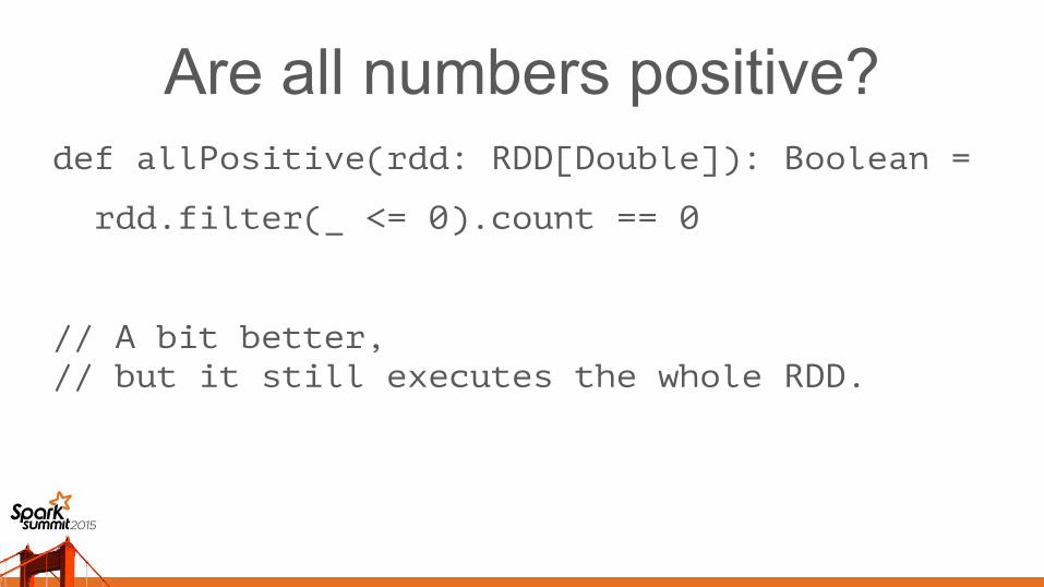
Are all numbers positive?def allPositive(rdd: RDD[Double]): Boolean =

rdd.filter(_ <= 0).count == 0

// A bit better,// but it still executes the whole RDD.

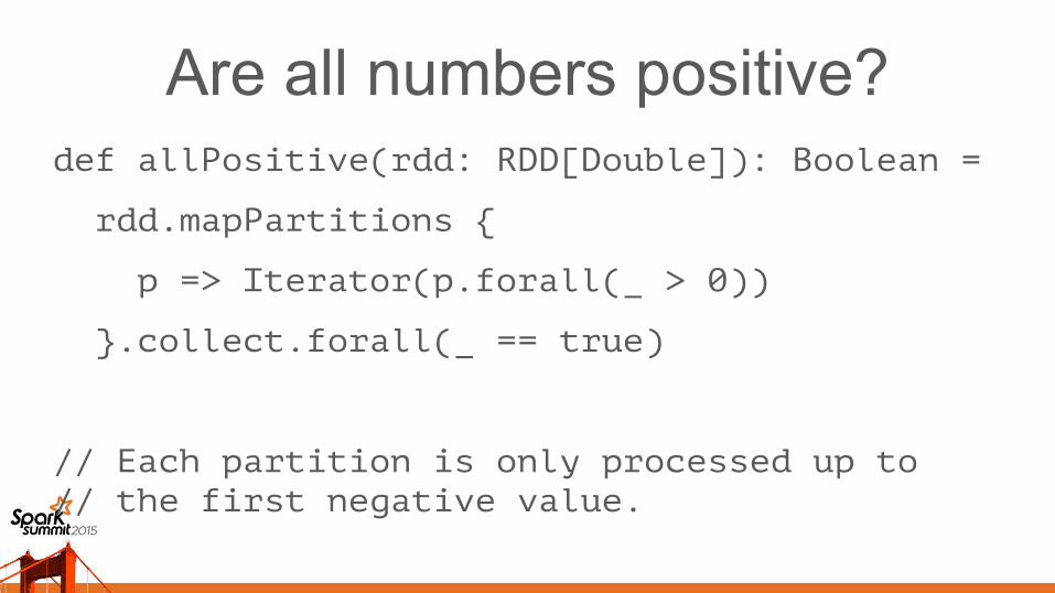
Are all numbers positive?def allPositive(rdd: RDD[Double]): Boolean =

rdd.mapPartitions {

p => Iterator(p.forall(_ > 0))

}.collect.forall(_ == true)

// Each partition is only processed up to// the first negative value.

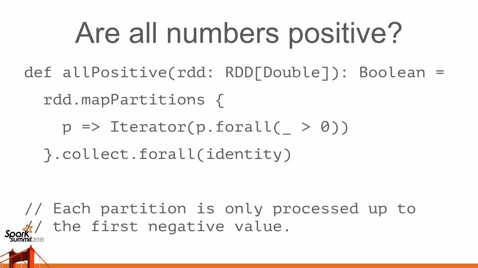
Are all numbers positive?def allPositive(rdd: RDD[Double]): Boolean =

rdd.mapPartitions {

p => Iterator(p.forall(_ > 0))

}.collect.forall(identity)

// Each partition is only processed up to// the first negative value.

Prefix samplingPartitions are sorted by the randomly assigned ID

Taking the first N elements is an unbiased sample

Lazy evaluation means the rest are not even computed

Used for histograms and bucketed views

Idea 4:

Lookup instead of filtering for small key sets

Restricted ID setsCannot use sampling when showing 5 vertices

Hard to explain why showing 5 million is faster

Partitions are already sorted

We can use binary search to look up attributes

Put partitions into arrays for random access

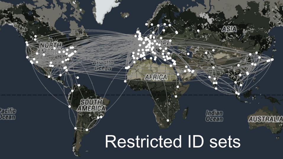
Restricted ID sets

SummaryColumn-oriented attributes

Small number of co-located, cached partitions

Sorted RDDs

Prefix sampling

Binary search-based lookup

Backup slides

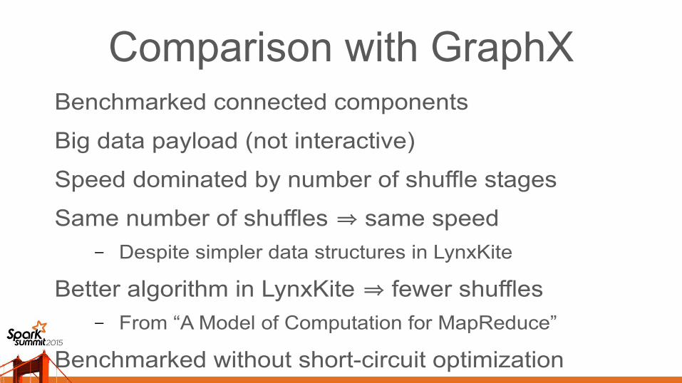
Comparison with GraphXBenchmarked connected components

Big data payload (not interactive)

Speed dominated by number of shuffle stages

Same number of shuffles ⇒ same speed– Despite simpler data structures in LynxKite

Better algorithm in LynxKite ⇒ fewer shuffles– From “A Model of Computation for MapReduce”

Benchmarked without short-circuit optimization

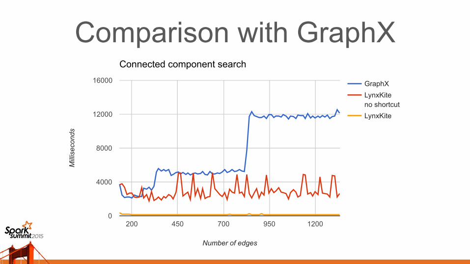
Connected component search

GraphX

LynxKiteno shortcut

LynxKite

200 450 700 950 12000

4000

8000

12000

16000

Number of edges

Mill

ise

con

ds

Comparison with GraphX

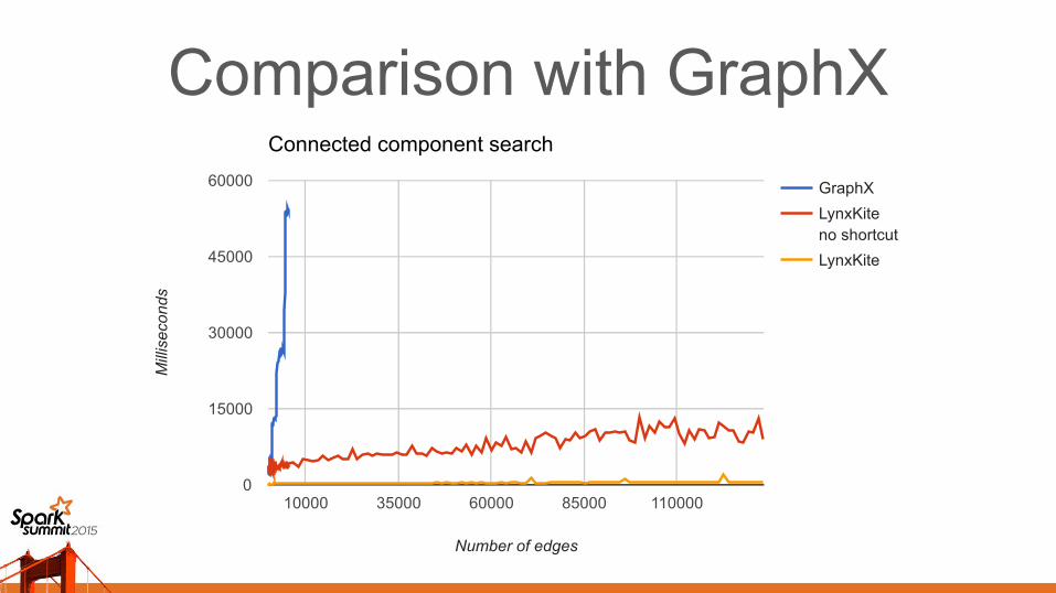
Connected component search

GraphX

LynxKiteno shortcut

LynxKite

10000 35000 60000 85000 1100000

15000

30000

45000

60000

Number of edges

Mill

ise

con

ds

Comparison with GraphX