Interactions Between PVS and Maple in Symbolic Analysis of Control Systems

Interactions Between PVS and Maple in

Symbolic Analysis of Control Systems

Ruth Hardy1 ,2

School of Computer ScienceUniversity of St Andrews

St Andrews, Scotland

Abstract

This paper presents a decision procedure for problems relating polynomial and transcendentalfunctions. The procedure applies to functions that are continuously differentiable with a finitenumber of points of inflection in a closed convex set. It decides questions of the form ‘is f ∼ 0?’,where ∼∈ {=, >, <}. An implementation of the procedure in Maple and PVS exploits the existingMaple, PVS and QEPCAD connections. It is at present limited to those twice differentiablefunctions whose derivatives are rational functions (rationally differentiable). This procedure isparticularly applicable to the analysis of control systems in determining important properties suchas stability.

Keywords: reliable mathematics, formal methods, quantifier elimination, control systems,Maple-PVS, QEPCAD

1 Introduction

Many problems in the fields of mathematics, computer science and control en-gineering can be reduced to decision and quantifier elimination problems [7],[14], [20], often involving trigonometric and transcendental functions; prob-lems such as algebraic surface intersection and display; robot motion planning

1 Thanks go to Ursula Martin and Richard Boulton for their help and guidance, especiallyin the early stages of this work, also to Roy Dyckhoff and Steve Linton for their continuinghelp and guidance. Additional thanks go to John Hall, Rick Hyde and Yoge Patel forsharing their insights into control engineering, and to Rob Arthan, Tom Kelsey and ColinO’Halloran for many helpful discussions.2 Email: [email protected]

Electronic Notes in Theoretical Computer Science 151 (2006) 111–125

1571-0661/$ – see front matter © 2006 Elsevier B.V. All rights reserved.

www.elsevier.com/locate/entcs

doi:10.1016/j.entcs.2005.11.026

mailto:[email protected]

http://www.elsevier.com/locate/entcs

(where the aim is to determine whether a number of objects, whose physicalattributes and range of motion can be described algebraically, can move fromsome initial configuration to reach some final configuration); stability analy-sis using the von Neumann condition for the stability of difference schemes.Quantifier elimination algorithms for real closed fields (RCF) have been de-veloped [6], [17], [18] and various algorithms have been suggested for specialtypes of problems involving trigonometric or transcendental functions [2], [21]but these are limited to very specific problems and often do not include sup-port for inverse trigonometric or transcendental functions such as arctan orthe natural logarithm, which are important in control engineering.

A problem arising in analysis of control systems is to decide if a givenfunction is greater than another in an interval [10]. In this paper we presenta decision procedure for problems of this type for functions f : R

2 → R thatare continuously differentiable with a finite number of points of inflection in aclosed convex set (a set such that every element that lies between two mem-bers of the set is a member of the set and the boundary points of the set aremembers of it). The procedure requires efficient reliable symbolic manipula-tion of mathematical formulae and exact numerical calculation. No existingindividual tool has all of these qualities. Computer algebra systems (CASs)are excellent at symbolic manipulation and often provide powerful methodsfor numerical calculations, however, they cannot guarantee correct results;formal theorem provers (TPs) can guarantee correct results but are inefficientfor automatic symbolic manipulation and numerical calculations. There hasbeen much interest in the development of systems that provide the power of aCAS and the rigour of a TP. Systems of this type fall into two main categories;computational support for TPs and formal support for CASs. Systems such asMaple–HOL [11] and Maple–Isabelle [3] provide links between the TPs HOLand Isabelle and the CAS Maple, allowing the TPs to call upon the compu-tational power of Maple under appropriate circumstance to increase efficiencyof proof or proof search; Maple–PVS [1] provides a link between Maple andthe TP PVS, allowing Maple to call upon the theorem proving power of PVSto increase reliability of its results; the Omega proof development system [15]supports the integration of computer algebra into mechanised reasoning sys-tems at the proof planning stage; Redlog [8], Analytica [4] and Theorema[5] extend CASs with support for formal theorem proving. A prototype toolimplementing the decision procedure has been developed in the Maple–PVSsystem, taking advantage of the reliable efficient mathematics it provides.

The formulae for which the decision procedure is applicable are classifiedin Section 2 of this paper, in terms of a fragment of a first order logic L for thereals. Various important geometric properties of curves are given in Section 3.

R. Hardy / Electronic Notes in Theoretical Computer Science 151 (2006) 111–125112

In Section 4 the procedure for deciding sentences of the language L based onthe geometric properties of curves is described. In Section 5 the practical issuesassociated with the automation of the procedure are discussed and a prototypetool combining Maple, PVS and QEPCAD is presented to demonstrate howcomputer algebra, theorem proving and quantifier elimination systems canbe combined to automate the procedure for sentences of L containing onequantified variable. Section 6 presents a simple example of the usage of thismethod in the analysis of a control system. Finally, conclusions and directionsfor further work are presented in Section 7.

2 Classification

A closed convex set is a subset of Rn, such that every element that lies on the

line between two members of the set is also a member of the set and all limitpoints of the set are also members of it. In the one dimensional case, a setD ⊆ R is a closed convex set if and only if D is a closed interval.

A continuously differentiable term is a function whose derivative existsand is continuous, i.e, it is an expression of the form f(x) such that ∇f existsand is a vector of continuous terms. Rational terms are a specialised formof continuously differentiable terms and are quotients of polynomials in thevariables xi with real coefficients ai. If these coefficients are non–algebraic thenthey are described in terms of intervals (ail, aiu) with real algebraic bounds,in which they lie. Linear terms are a specialised form of rational terms, suchthat they are linear in all variables, i.e, they are expressions of the form a0 +∑n

i=0aixi where a0, ai are real algebraic numbers and xi are real variables. A

rationally differentiable term is a specialised form of continuously differentiableterm, such that it is differentiable and all partial derivatives are rational terms,i.e, it is an expression of the form f(x) such that ∇f exists and is a vector ofrational terms. A finitely inflective term is a continuously differentiable termwith a finite number of regions of convexity and/or concavity.

An atomic formula in the language L is an equation or inequality involv-ing a finitely inflective term over some closed convex set, x ∈ D ⇒ f(x) ∼ 0where D is a closed convex set of R

n, f : Rn → R and ∼∈ {=, >, <}.

Arbitrary formulae are obtained by iterated application of the propositionaloperators ∨, ∧, ¬ and the quantifiers ∃, ∀ with respect to the variable xi.Every formula can be rewritten in equivalent prenex normal form. If all oc-currences of x in a formula φ are quantified then φ is a closed formula and,given the natural interpretation of formulae over reals, is either true or false.

R. Hardy / Electronic Notes in Theoretical Computer Science 151 (2006) 111–125 113

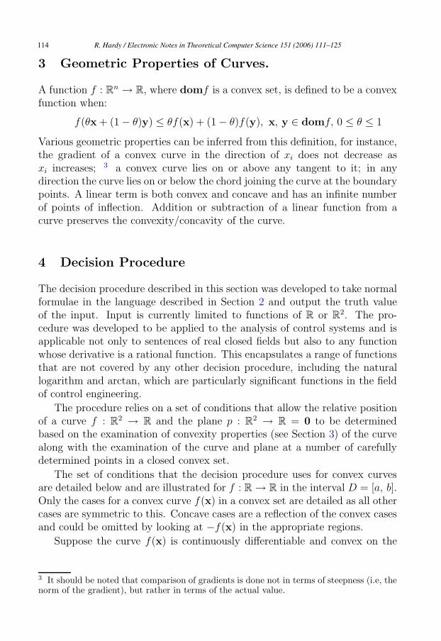
3 Geometric Properties of Curves.

A function f : Rn → R, where domf is a convex set, is defined to be a convex

function when:

f(θx + (1 − θ)y) ≤ θf(x) + (1 − θ)f(y), x, y ∈ domf, 0 ≤ θ ≤ 1

Various geometric properties can be inferred from this definition, for instance,the gradient of a convex curve in the direction of xi does not decrease asxi increases; 3 a convex curve lies on or above any tangent to it; in anydirection the curve lies on or below the chord joining the curve at the boundarypoints. A linear term is both convex and concave and has an infinite numberof points of inflection. Addition or subtraction of a linear function from acurve preserves the convexity/concavity of the curve.

4 Decision Procedure

The decision procedure described in this section was developed to take normalformulae in the language described in Section 2 and output the truth valueof the input. Input is currently limited to functions of R or R

2. The pro-cedure was developed to be applied to the analysis of control systems and isapplicable not only to sentences of real closed fields but also to any functionwhose derivative is a rational function. This encapsulates a range of functionsthat are not covered by any other decision procedure, including the naturallogarithm and arctan, which are particularly significant functions in the fieldof control engineering.

The procedure relies on a set of conditions that allow the relative positionof a curve f : R

2 → R and the plane p : R2 → R = 0 to be determined

based on the examination of convexity properties (see Section 3) of the curvealong with the examination of the curve and plane at a number of carefullydetermined points in a closed convex set.

The set of conditions that the decision procedure uses for convex curvesare detailed below and are illustrated for f : R → R in the interval D = [a, b].Only the cases for a convex curve f(x) in a convex set are detailed as all othercases are symmetric to this. Concave cases are a reflection of the convex casesand could be omitted by looking at −f(x) in the appropriate regions.

Suppose the curve f(x) is continuously differentiable and convex on the

3 It should be noted that comparison of gradients is done not in terms of steepness (i.e, thenorm of the gradient), but rather in terms of the actual value.


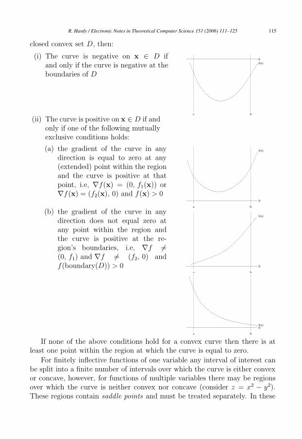
closed convex set D, then:

(i) The curve is negative on x ∈ D ifand only if the curve is negative at theboundaries of D

0f(x)

a b

(ii) The curve is positive on x ∈ D if andonly if one of the following mutuallyexclusive conditions holds:

(a) the gradient of the curve in anydirection is equal to zero at any(extended) point within the regionand the curve is positive at thatpoint, i.e, ∇f(x) = (0, f1(x)) or∇f(x) = (f2(x), 0) and f(x) > 0

f(x)

a b

0

(b) the gradient of the curve in anydirection does not equal zero atany point within the region andthe curve is positive at the re-gion’s boundaries, i.e, ∇f �=(0, f1) and ∇f �= (f2, 0) andf(boundary(D)) > 0 0

f(x)

ba

f(x)

ba

0

If none of the above conditions hold for a convex curve then there is atleast one point within the region at which the curve is equal to zero.

For finitely inflective functions of one variable any interval of interest canbe split into a finite number of intervals over which the curve is either convexor concave, however, for functions of multiple variables there may be regionsover which the curve is neither convex nor concave (consider z = x2 − y2).These regions contain saddle points and must be treated separately. In these


regions the function is convex in some directions and concave in others. Themaximum and minimum values for the function in these regions lie on theboundaries, and the sign of the function on these boundaries can be used todetermine whether the curve is positive or negative in the region.

In order to use the conditions described here to decide sentences of thelanguage described in Section 2 the closed convex set must be split into regionsover which the curve is either convex, concave or contains a saddle point.

The decision procedure takes sentence φ in prenex normal form in thelanguage described in Section 2 and performs the following steps:

Step 1: Convert existential quantification in φ to universal quantificationgiving φ′. This is a syntactic conversion to simplify the algorithm: ∃x.P (x)becomes ¬∀x.¬P (x)Step 2: Take each atomic formula fi ∼i 0 from φ′ and determine the regionsDij of convexity, concavity and those containing saddle points for fi.Step 3: For each of the regions Dij within domfi apply the appropriate casefrom the set of conditions. If the correct conditions hold for all these regionsthen the i-th atomic formula has the value TRUE. If the condition fails tohold for any of the regions then the formula has the value FALSE.Step 4: Construct the truth value for the sentence φ′ (and thus φ) by applyingthe propositional operators within it to the truth values of Step 3.

The set of conditions presented in this section are applicable to functionsthat are finitely inflective, that is functions that are differentiable with a con-tinuous derivative and a finite number of regions in which the curve is convexor concave. In practice this requirement is strengthened to finitely inflectiverationally differentiable functions.

Proofs in PVS of coverage of these cases exists along with proof of ter-mination of the procedure given that convexity is known and the number ofregions in which the curve is convex or concave is finite in a closed convex set.

5 Implementation in Maple–PVS

In order to implement this procedure one must be able to reliably calculate thepoints of inflection of continuously differentiable functions, the convexity of thecorresponding curve and the sign of the curve at given points. This requiresnot only powerful symbolic manipulation whose results are guaranteed correctbut also validated numerical calculation.

Computer Algebra Systems (CASs) provide a powerful method for sym-bolic manipulation and analysis of mathematical formulae and are ideal for


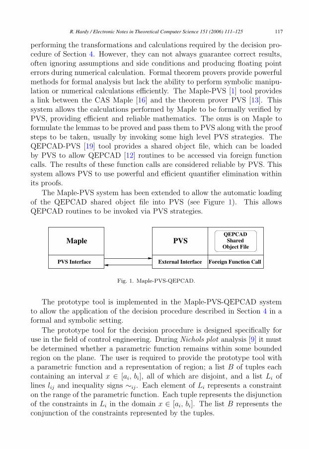
performing the transformations and calculations required by the decision pro-cedure of Section 4. However, they can not always guarantee correct results,often ignoring assumptions and side conditions and producing floating pointerrors during numerical calculation. Formal theorem provers provide powerfulmethods for formal analysis but lack the ability to perform symbolic manipu-lation or numerical calculations efficiently. The Maple-PVS [1] tool providesa link between the CAS Maple [16] and the theorem prover PVS [13]. Thissystem allows the calculations performed by Maple to be formally verified byPVS, providing efficient and reliable mathematics. The onus is on Maple toformulate the lemmas to be proved and pass them to PVS along with the proofsteps to be taken, usually by invoking some high level PVS strategies. TheQEPCAD-PVS [19] tool provides a shared object file, which can be loadedby PVS to allow QEPCAD [12] routines to be accessed via foreign functioncalls. The results of these function calls are considered reliable by PVS. Thissystem allows PVS to use powerful and efficient quantifier elimination withinits proofs.

The Maple-PVS system has been extended to allow the automatic loadingof the QEPCAD shared object file into PVS (see Figure 1). This allowsQEPCAD routines to be invoked via PVS strategies.

External Interface Foreign Function CallPVS Interface

Maple PVSObject File

QEPCADShared

Fig. 1. Maple-PVS-QEPCAD.

The prototype tool is implemented in the Maple-PVS-QEPCAD systemto allow the application of the decision procedure described in Section 4 in aformal and symbolic setting.

The prototype tool for the decision procedure is designed specifically foruse in the field of control engineering. During Nichols plot analysis [9] it mustbe determined whether a parametric function remains within some boundedregion on the plane. The user is required to provide the prototype tool witha parametric function and a representation of region; a list B of tuples eachcontaining an interval x ∈ [ai, bi], all of which are disjoint, and a list Li oflines lij and inequality signs ∼ij . Each element of Li represents a constrainton the range of the parametric function. Each tuple represents the disjunctionof the constraints in Li in the domain x ∈ [ai, bi]. The list B represents theconjunction of the constraints represented by the tuples.


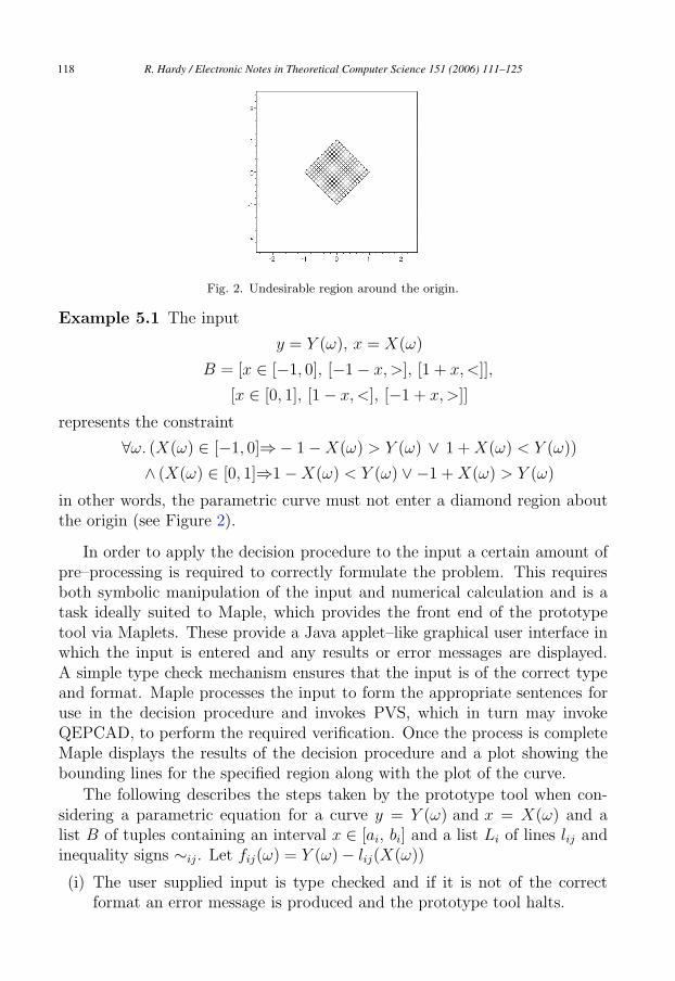
Fig. 2. Undesirable region around the origin.

Example 5.1 The input

y = Y (ω), x = X(ω)

B = [x ∈ [−1, 0], [−1 − x, >], [1 + x, <]],

[x ∈ [0, 1], [1 − x, <], [−1 + x, >]]

represents the constraint

∀ω. (X(ω) ∈ [−1, 0]⇒− 1 − X(ω) > Y (ω) ∨ 1 + X(ω) < Y (ω))

∧ (X(ω) ∈ [0, 1]⇒1 − X(ω) < Y (ω) ∨ −1 + X(ω) > Y (ω)

in other words, the parametric curve must not enter a diamond region aboutthe origin (see Figure 2).

In order to apply the decision procedure to the input a certain amount ofpre–processing is required to correctly formulate the problem. This requiresboth symbolic manipulation of the input and numerical calculation and is atask ideally suited to Maple, which provides the front end of the prototypetool via Maplets. These provide a Java applet–like graphical user interface inwhich the input is entered and any results or error messages are displayed.A simple type check mechanism ensures that the input is of the correct typeand format. Maple processes the input to form the appropriate sentences foruse in the decision procedure and invokes PVS, which in turn may invokeQEPCAD, to perform the required verification. Once the process is completeMaple displays the results of the decision procedure and a plot showing thebounding lines for the specified region along with the plot of the curve.

The following describes the steps taken by the prototype tool when con-sidering a parametric equation for a curve y = Y (ω) and x = X(ω) and alist B of tuples containing an interval x ∈ [ai, bi] and a list Li of lines lij andinequality signs ∼ij . Let fij(ω) = Y (ω) − lij(X(ω))

(i) The user supplied input is type checked and if it is not of the correctformat an error message is produced and the prototype tool halts.


(ii) Maple calculates, rewrites and simplifies the derivative and second deriva-tive of the parametric equation with respect to x. Since the decisionprocedure relies upon the convexity of the curve and thus the sign of thesecond derivative it is important to confirm that Maple has calculatedthis correctly and has not ignored any important side conditions. Maplecalls PVS to confirm that the function is well defined and is twice differ-entiable. If PVS fails to provide the required proof then the prototypetool produces an appropriate error message and halts.

(iii) The intervals [ai, bi] are in term of x but the procedure will require theseintervals to be in terms of ω, i,e. [ai, bi] = [X(ωik), X(ωik+1)]. To cal-culate these intervals in terms of ω all real solutions to ai = X(ωik) orbi = X(ωik) must be found, then by looking at a point between each ωik

and ωik+1 the corresponding intervals can be determined. Since Mapledoes this using numerical calculation it can suffer from the problem ofinexact arithmetic caused by floating point error and may fail to find allsolutions.To ensure that all solutions have been found it must be shown that the so-lutions found by Maple actually are approximate solutions and that thereare no other solutions within the intervals [ai, bi]. Letting Di representsmall intervals around each of Maple’s solution the decision procedure isapplied to

∃ω. ω ∈ Di ⇒ X(ω) = ai ∨ X(ω) = bi(1)

to ensure that there are solutions in the intervals and

∀ω1, ω2. ω1 ∈ Di ∧ ω2 ∈ Di ⇒(2)

(X(ω1) = ai ∨ X(ω1) = bi) ∧ (X(ω2) = ai ∨ X(ω2) = bi) ⇒ ω1 = ω2

to ensure that there is only one solution in each intervals. The decisionprocedure is also applied to

∀ω. ω /∈ D ⇒ X(ω) �= ai ∧ X(ω) �= bi(3)

where D is the set of reals x such that x ∈ D0 ∨ x ∈ D1 ∨ . . ., to ensurethat there are no solutions other than those found by Maple. If this failsthe prototype tool produces an appropriate error message and halts.To compensate for Maple’s inexact arithmetic the solutions are adjustedby a small value to give ‘safe’ bounds for the interval for example ifMaple calculates ωik and ωik+1 such that [ai, bi] [X(ωik), X(ωik+1)]then Maple adjust by some δ such that [ai, bi] ⊆ [X(ωik−δ), X(ωik+1+δ)].It is important that this condition holds so Maple calls PVS to verify thesolutions. If PVS fails to provide the required proof then the prototypetool produces an appropriate error message and halts.


(iv) Maple calculates the points of inflection of fij, including any points atwhich it becomes vertical, in the intervals [ωik − δ, ωik+1 + δ]. This isachieved using numerical methods to find points at which the secondderivative of fij in terms of x (which is the same as the second derivativeof the parametric curve calculated in Step ii) is zero and as a conse-quence is subject to errors due to inexact arithmetic. To avoid this prob-lem Maple calculates small intervals [pikm − δ, pikm + δ] in which thesepoints lie (referred to as intervals of inflection). PVS is called to confirmnot only that these intervals contain true points of inflection rather thanpoints of zero curvature between two regions both strictly convex or con-cave but also that each of these points is the only point of inflection in[pikm − δ, pikm + δ] and that the derivative of fij does not equal zero in[pikm − δ, pikm + δ] unless it is exactly at the point of inflection. This is arelatively difficult problem for PVS to solve but since the derivative andsecond derivative of fij are rational it is ideal for quantifier elimination.PVS uses the QEPCAD-PVS link to invoke the QEPCAD strategies toverify Maple’s results. If PVS fails to provide the required proof then theprototype tool produces an appropriate error message and halts.

(v) The intervals [ωik − δ, ωik+1 + δ] are split into [ωik − δ, pikm − δ] [pikm −δ, pikm + δ] [pikm + δ, ωik+1 + δ] over which the curve is either convex orconcave, or is an interval of inflection.

(vi) Maple formulates the lemmas to be solved by PVS in the form λω ∈ [a, b].fij(ω) ∼ij 0 using the inequality sign ∼ij and the intervals calculated inthe previous step. PVS is called by Maple to prove these lemmas andin essence determine whether the desired case from the set of conditionsholds. In the case of intervals of inflection the truth of the sentence is notfound using one of the cases of Section 4 but is determined, if necessary,by examining the bounds of the interval, since due to the nature of theseintervals the maximum and minimum of fij must lie on the bounds. Thetruth value for atomic formula fij ∼ij 0 is built up from the conjunctionof each of the truth values of the corresponding lemmas.

(vii) The truth of the formulae represented by each Li is built up from thedisjunction of the truth values of each fij ∼ij 0. The truth of the formularepresented by B is then built up from the conjunction of the truth valuesof each Li. The prototype tool produces an appropriate message statingwhether the formula is true or false.

(viii) Maple produces a plot of the lines and the parametric plot of the curve.

PVS uses custom built libraries containing lemmas concerning the differ-entiability of various functions important in control system analysis, such as


arctan, natural logarithm, logarithm to the base 10, arbitrary rational func-tions and parametric functions, along with high level strategies and externalfunction calls to QEPCAD to provide the proofs required in the prototypetool. These libraries contain definitions of the natural logarithm and arctanas Taylor series, which allows bounds on the value of these functions for anygiven input to be defined.

6 A Simple Example

In this section we present a simple example of how one might use the decisionprocedure presented in Section 4 and the implementation presented in Section5 to determine formally whether a curve meets a line. The given exampleis representative of the form that arise in Nichols Plot analysis of controlsystems. It is a particularly interesting example as the curve contains intervalsof convexity and concavity, points at which the curve is vertical and multipleintervals in terms of ω corresponding to a single interval in terms of x.

Consider the following bounding lines and parametric equation (see Figure3):

B = x ∈ [−1.5, 0.5], [[55 + 8x, >], [65 − 12x, <]]

Y (ω) =10 ln(p) − 20 ln(ω6 + 5ω4 + 60ω2 + 16)

ln(10)

X(ω) = arctan

(797ω6 + 14382ω4 + 755ω2 − 3194

800ω8 + 4803ω6 + 12054ω4 − 1597ω2 + 55

)

where ω ≥ 0, and

p = 640000ω16 + 7684800ω14 + 42990418ω12 + 136160432ω10

338091528ω8 − 21346562ω6 − 87425842ω4 − 4998610ω2 + 10204661

Maple calculates the derivative f ′ and second derivative f ′′ of the givenparametric function. Considering ln(10) as some real constant in the range(2.302585090, 2.302585100), both the derivative and second derivative are ra-tional functions. Maple calls PVS to confirm that the parametric function istwice differentiable and that the derivatives are as specified by Maple. Thisis a relatively simple task for PVS, which uses the custom built libraries andpowerful general purpose simplification and rewrite strategies such as GRIND

to provide the relevant proofs.

The next step is to determine the intervals over ω that correspond toX(ω) ∈ [−1.5, 0.5]. Maple calculates all solutions for X(ω1j) = −1.5 andX(ω1j) = 0.5 discarding all non–real solutions and all those that are notin the domain of the parametric function (in this case negative solutions).


This leaves three solutions ω1,1 = 0.4231452940, ω1,2 = 0.7664324880 andω1,3 = 1.631039454, giving four potential corresponding intervals:

[−∞, ω1,1], [ω1,1, ω1,2], [ω1,2, ω1,3], [ω1,3, ∞]

Maple confirms that these are indeed approximate solutions and that theyare the only solutions in the domain of the function by letting δ = 0.001 andapplying the decision procedure to

∃ω. ω ∈ [ω1,i − δ, ω1,i + δ] ⇒ X(ω) = −1.5 ∨ X(ω) = 0.5

to determine the existence of solutions,

∀ω1, ω2. ω1 ∈ [ω1,i − δ, ω1,i + δ] ∧ ω2 ∈ [ω1,i − δ, ω1,i + δ] ⇒

(X(ω1) = −1.5 ∨ X(ω1) = 0.5) ∧ (X(ω2) = −1.5 ∨ X(ω2) = 0.5)

⇒ ω1 = ω2

to determine the uniqueness of each solution in each interval and

∀ω. ω ≥ 0 ∧ ω /∈ [ω1,1 − δ, ω1,1 + δ] ∧ ω /∈ [ω1,2 − δ, ω1,2 + δ]∧

ω /∈ [ω1,3 − δ, ω1,3 + δ] ⇒ X(ω) �= −1.5 ∧ X(ω) �= 0.5

to determine that all solutions were found. Since none of these problemsinvolve parametric equations the application of the decision procedure is muchsimpler and does not require the application of step iii in Section 5. Also, sincethere are no points of inflection in the first two problems (nor are there likelyto be in most cases since the intervals of interest are so small) the applicationof the procedure is again simplified requiring no splitting of the intervals intosubinterval as described in steps iv and v in Section 5.

Once it has been confirmed that the Solutions found by Maple are in-deed correct a point within each of the intervals is examined, determiningthat [ω1,1, ω1,2], and [ω1,3, ∞] correspond to the interval X(ω) ∈ [−1.5, 0.5].To ensure the bounds on these intervals are ‘safe’ Maple adjusts them byδ = 0.01; lower bounds are reduced by δ, upper bounds are increased byδ. At this point Maple calls PVS to confirm its calculations are correct, i.e,that [−1.5, 0.5] ⊆ [X(ω1,1 − δ), X(ω1,2 + δ)] and that [limω→∞ X(ω), 0.5] ⊆[limω→∞ X(ω), X(ω1,3 + δ)]. PVS uses custom built libraries and calls toQEPCAD to ensure this safety property.

Maple calculates the points of inflection of the parametric function, in-cluding points at which it becomes vertical by determining points at whichthe denominator and numerator of the second derivative equal zero. Dis-carding all points not within any interval of interest leaves a single pointω1,3,1 = 1.894587409 within the interval [limω→∞ X(ω), X(ω1,3 + δ)]. Maplecalculates the interval of inflection [ω1,3,1−δ, ω1,3,1+δ] and invokes PVS, whichuses the QEPCAD strategies to prove that there is only one point of inflection


in the interval and that there is no point at which the derivative is equal tozero

∃ω ∈ [ω1,3,1 − δ, ω1,3,1 + δ].∀ω2 ∈ [ω1,3,1 − δ, ω1,3,1 + δ].

(f ′′(ω) = 0 ∧ f ′′(ω2) = 0)⇒ω = ω2

∀ω ∈ [ω1,3,1 − δ, ω1,3,1 + δ]. f ′(ω) − 8 �= 0

∀ω ∈ [ω1,3,1 − δ, ω1,3,1 + δ]. f ′(ω) + 12 �= 0

Maple then formulates the appropriate lemmas

λω ∈ [ω1,1 − δ, ω1,2 + δ].(4)

Y (ω) − l1,1(X(ω)) ∼1,1 0 ∨ Y (ω) − l1,2(X(ω)) ∼1,2 0

λω ∈ [ω1,3 − δ, ω1,3,1 − δ].(5)

Y (ω) − l1,1(X(ω)) ∼1,1 0 ∨ Y (ω) − l1,2(X(ω)) ∼1,2 0

λω ∈ [ω1,3,1 − δ, ω1,3,1 + δ].(6)

Y (ω) − l1,1(X(ω)) ∼1,1 0 ∨ Y (ω) − l1,2(X(ω)) ∼1,2 0

λω ∈ [ω1,3,1 + δ, ∞].(7)

Y (ω) − l1,1(X(ω)) ∼1,1 0 ∨ Y (ω) − l1,2(X(ω)) ∼1,2 0

Each of these lemmas correspond either to one of the cases used in the decisionprocedure or to an interval of inflection. For lemmas 4, 5 and 7 PVS uses theappropriate case from the decision procedure to form a proof, the proof oflemma 6 follows directly from the truth of lemmas 5 and 7. This completesthe calculations for the decision procedure.

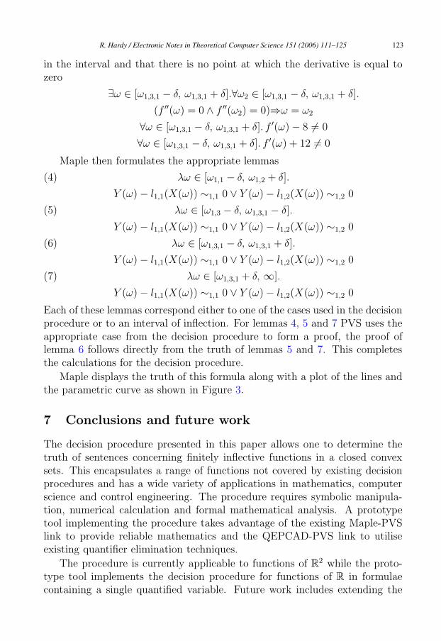
Maple displays the truth of this formula along with a plot of the lines andthe parametric curve as shown in Figure 3.

7 Conclusions and future work

The decision procedure presented in this paper allows one to determine thetruth of sentences concerning finitely inflective functions in a closed convexsets. This encapsulates a range of functions not covered by existing decisionprocedures and has a wide variety of applications in mathematics, computerscience and control engineering. The procedure requires symbolic manipula-tion, numerical calculation and formal mathematical analysis. A prototypetool implementing the procedure takes advantage of the existing Maple-PVSlink to provide reliable mathematics and the QEPCAD-PVS link to utiliseexisting quantifier elimination techniques.

The procedure is currently applicable to functions of R2 while the proto-

type tool implements the decision procedure for functions of R in formulaecontaining a single quantified variable. Future work includes extending the


Fig. 3. Parametric plot of Y against X showing lines l1,1 and l1,2.

decision procedure to functions of higher dimensions, improving efficiency ofthe current prototype tool and extending its capabilities to include decidingsentences involving functions of higher dimensions with a larger number ofquantified variables.

References

[1] A Adams, M Dunstan, H Gottliebsen, T Kelsey, U Martin, and S Owre. Computer algebrameets automated theorem proving: Integrating Maple and PVS. In R. J Boulton and P. BJackson, editors, Proceedings of the 14th International Conference on Theorem Proving inHigher Order Logics (TPHOLs 2001), volume 2152 of Lecture Notes in Computer Science,pages 27–42. Springer-Verlag, 2001.

[2] H Anai and V Weispfenning. Deciding linear–trigonometric problems. In C Traverso,editor, ISSAC ’00: Proceedings of the 2000 international symposium on Symbolic and algebraiccomputation, pages 14–22. ACM Press, 2000.

[3] C Ballarin, K Homann, and J Calmet. Theorems and algorithms: an interface between isabelleand maple. In A. H. M Levelt, editor, ISSAC ’95: Proceedings of the 1995 internationalsymposium on Symbolic and algebraic computation, pages 150–157. ACM Press, 1995.

[4] A Bauer, E Clark, and X Zhao. Analytica – an experiment in combining theorem proving andsymbolic computation. Journal of Automated Reasoning, 21(3):295–325, 1998.

[5] B Buchberger, T Jebelean, F Kriftner, M Marin, E Tomuta, and D Vasaru. A survey of thetheorema project. In W Kuechlin, editor, ISSAC ’97: Proceedings of the 1997 internationalsymposium on Symbolic and algebraic computation, pages 384–391. ACM Press, 1997.

[6] B. F Caviness and J. R Johnson, editors. Quantifier Elimination and Cylindrical AlgebraicDecomposition. Springer Wien NewYork, 1998.

[7] A Dolzmann. Solving geometric problems with real quantifier elimination. Technical ReportRep. MIP-9903, Universitat Passau, 1999.

[8] A Dolzmann and T Sturm. Redlog: Computer algebra meets computer logic. ACM SIGSAMBulletin, 31(2):2–9, 1997.


[9] R. C Dorf and R. H Bishop. Modern Control Systems. Prentice-Hall, ninth edition, 2001.

[10] Action Group FM(AG08). Robust flight control design challenge problem formulation andmanual: the high incidence research model (HIRM). Technical Report TP-088-4, version 3,Group for Aeronautical Research and Technology in Europe (GARTEUR), 1997.

[11] J Harrison and L Thery. Reasoning about the reals: the marriage of HOL and maple.In A Voronkov, editor, Logic programming and automated reasoning: proceedings of the 4thinternational conference, LPAR ’93, volume 698 of Lecture Notes in Computer Science, pages351–359. Springer-Verlag, 1993.

[12] H Hong. Qepcad. Available at http://www.cs.usna.edu/∼qepcad/B/QEPCAD.html.

[13] SRI International. PVS. Available at http://pvs.csi.sri.com.

[14] M Jirstrand. Nonlinear control system design by quantifier elimination. Journal of SymbolicComputation, 24(2):137–152, 1997.

[15] M Kerber, M Kohlhase, and V Sorge. Integrating computer algebra into proof planning.Journal of Automated Reasoning, 21(3):327–355, 1998.

[16] Maplesoft. Maple. Available at http://www.maplesoft.com/products/maple/ .

[17] A Seidenberg. A new decision method for elementary algebra. Annals of Math, 60:365–374,1954.

[18] A Tarski. A Decision method for elementary algebra and geometry. University of CaliforniaPress, 1951.

[19] A Tiwari. PVS-QEPCAD. Available athttp://www.csl.sri.com/users/tiwari/qepcad.html .

[20] V Weispfenning. Simulation and optimization by quantifier elimination. Journal of SymbolicComputation, 24(2):189–208, 1997.

[21] V Weispfenning. Deciding linear-exponential problems. SIGSAM Bullettin, 34(1):30–31, 2000.


http://www.cs.usna.edu/~qepcad/B/QEPCAD.html

http://pvs.csi.sri.com

http://www.maplesoft.com/products/maple/

http://www.csl.sri.com/users/tiwari/qepcad.html

Interactions Between PVS and Maple in Symbolic Analysis of Control Systems

Documents

Transcript of Interactions Between PVS and Maple in Symbolic Analysis of Control Systems