DI

SC

US

SI

ON

P

AP

ER

S

ER

IE

S

Forschungsinstitut zur Zukunft der ArbeitInstitute for the Study of Labor

Interactions between Private and Public Sector Wages

IZA DP No. 5322

November 2010

António AfonsoPedro Gomes

Interactions between Private

and Public Sector Wages

António Afonso European Central Bank,

ISEG/TULisbon and UECE

Pedro Gomes Universidad Carlos III de Madrid

and IZA

Discussion Paper No. 5322 November 2010

IZA

P.O. Box 7240 53072 Bonn

Germany

Phone: +49-228-3894-0 Fax: +49-228-3894-180

E-mail: iza@iza.org

Any opinions expressed here are those of the author(s) and not those of IZA. Research published in this series may include views on policy, but the institute itself takes no institutional policy positions. The Institute for the Study of Labor (IZA) in Bonn is a local and virtual international research center and a place of communication between science, politics and business. IZA is an independent nonprofit organization supported by Deutsche Post Foundation. The center is associated with the University of Bonn and offers a stimulating research environment through its international network, workshops and conferences, data service, project support, research visits and doctoral program. IZA engages in (i) original and internationally competitive research in all fields of labor economics, (ii) development of policy concepts, and (iii) dissemination of research results and concepts to the interested public. IZA Discussion Papers often represent preliminary work and are circulated to encourage discussion. Citation of such a paper should account for its provisional character. A revised version may be available directly from the author.

IZA Discussion Paper No. 5322 November 2010

ABSTRACT

Interactions between Private and Public Sector Wages* We examine the interactions between public and private sector wages per employee in OECD countries. The growth of public sector wages and of public sector employment positively affects the growth of private sector wages. Moreover, total factor productivity, the unemployment rate and the degree of urbanisation are also important determinants of private sector wage growth. With respect to public sector wage growth, we find that it is influenced by fiscal conditions in addition to private sector wages. We then set up a dynamic labour market equilibrium model with two sectors, search and matching frictions and exogenous growth to understand the interaction mechanisms. The model is quantitative consistent with the main estimation findings. JEL Classification: E24, E62, H50 Keywords: public sector wages, private sector wages, employment, fiscal policy Corresponding author: António Afonso European Central Bank Directorate General Economics Kaiserstrasse 29 D-60311 Frankfurt am Main Germany E-mail: antonio.afonso@ecb.europa.eu

* We are grateful to Frank Cowell, Marcelo Ferman, Chris Pissarides, Lukas Reiss, Ad van Riet, Jürgen von Hagen, and participants of the 40th Money, Macro and Finance Research Group annual conference (London) and of the Eurosystem Working Group of Public Finances Workshop (Paphos) for helpful comments on previous versions. The opinions expressed herein are those of the authors and do not necessarily reflect those of the European Central Bank or the Eurosystem. UECE is supported by FCT (Fundaçãao para a Ciência e a Tecnologia, Portugal), financed by ERDF and Portuguese funds. Gomes would like to thank the Fiscal Policies Division of the ECB for its hospitality and acknowledges financial support of FCT.

1 Introduction

The relevance of public wages for total government spending has increased gradually over the

past decades in several European countries. Apart from the importance that such a budgetary

item has for the development of public finances and for attaining budgetary objectives1, public

sector employment and wages play a key role in the labour market. In this context, the main

objective of this paper is to study one aspect of the relation between fiscal policy and the

labour market, namely the interaction between private and public sector wages.

First, we analyse the interactions between the wages in the two sectors empirically. We

examine the determinants of private sector wage growth, paying attention to the role of public

sector wage and employment growth, as well as other market related variables. Additionally,

we look at the determinants of public sector wage growth. Although there is evidence of some

pro-cyclicality of public wages (Lamo, Perez, and Schuknecht (2008)), their developments may

be less aligned with those of the private sector. For instance, public wages can also depend on

the fiscal position. In fact, Poterba and Rueben (1995) and Gyourko and Tracy (1989) find

that fiscal conditions affect wages of public employees at a local level. Moreover, they might

be used as an instrument for income policies, thus they can depend on political factors such

as the political alignment of the ruling party or election cycles. For instance, Matschke (2003)

finds evidence of systematic public wage increases prior to a federal election in Germany.

We develop our analysis for OECD countries for the period between 1973 and 2000. We

carefully discuss the econometric issues involved, particularly the problem of endogeneity,

and how we subsequently address them. In a nutshell, we find that a number of variables

affect private sector wage growth, for instance: changes in the unemployment rate (negative

relationship), total factor productivity growth and changes in the urbanisation rate. Moreover,

public sector wages and employment growth also affect private sector wage growth. A 1%

1According to the European Commission, the average share of public wages (compensation of employees)in general government total spending was around 23 per cent in 2007 for the European Union, that is, around11 percent of GDP. Interestingly, the public wages-to-total government spending ratio was 28 per cent in 2006in the US.

2

increase in public sector wages raises the wages in the private sector by 0.3 percent. Public

sector wage growth seems to respond mainly to private sector wage growth, but also to the

budget balance, the tax wedge and the position of the countries in the political spectrum.

Second, we set up a dynamic two-sector labour market equilibrium model in order to un-

derstand the interaction mechanisms. The model, that features search and matching frictions

in the labour market and exogenous growth, captures the essence of the interaction between

the wages in the two sectors. The government determines wage increases depending on the

expected growth rate of private sector wages and an error correction that depends on the

public-private wage differential. The long-run growth rate is determined in the private sector

and then spreads out to the public sector, but similar to other models that address this issue,

we also find that public sector wages and employment affect private sector wages.2

Public sector wages and employment impinge on private sector wages via three channels.

First, they affect the outside option of the unemployed, either by increasing the probability

of being hired (public sector employment) or by increasing the value of being employed in the

public sector (public sector wages). Therefore, they put pressure on wage bargaining. Second,

they both crowd out private sector employment which, due to the presence of diminishing

marginal productivity of labour, raises the average productivity. Finally, both public wages

and employment have to be financed by an increase in taxes, which will also affect the wages

paid by the firm. In addition, the model also features the effects from private sector wages

to public sector wages in response to technology shocks. Re-doing the empirical exercise with

simulated data, yields very similar coefficients to the ones estimated for the OECD countries.

The paper is organised as follows. In Section 2 we present the empirical setting and in

Section 3 we report and discuss the results. In Section 4 we present the theoretical model.

Section 5 summarises the main findings of the paper.

2See, for instance, Holmlund and Linden (1993), Algan, Cahuc, and Zylberberg (2002), and Ardagna (2007).

3

2 Empirical framework

In this section, we estimate the determinants of both private sector and public sector wages.

Our underlying idea is to estimate two different wage functions that link private and public

wages, while carefully addressing the problem of endogeneity between the two.

Most papers provide an aggregate perspective of the relation between the two wages fo-

cussing on wage levels per employee (see, for instance, Nunziata (2005), Jacobson and Ohlsson

(1994) and Friberg (2007)). However, we prefer to model the growth rates of real compen-

sation per employee to assess the behaviour of the two variables in the short run. Since we

have annual data, the use of growth rates eliminates the low frequency movements, but pre-

serves the movements at business cycle frequency, which we are more interested in uncovering

(Abraham and Haltiwanger (1995)).

In the long-run it is natural that the two variables are cointegrated with a slope coefficient

of one, if not one would observe a constant divergence of the wages in the two sectors. 3 This

does not exclude differences in the levels of the wages, but simply that these differences do

not show a trend. In fact, we observe a public sector wage premium or a gap, either due to

different skills composition of employment or because of barriers between the two sectors.

2.1 Empirical specification for private sector wages

Our baseline wage function for the developments in private sector salaries is given by

ωpit = αi + δpωpit−1 + θpXpit + πpZp

it + κpEit−1 + µit. (1)

In (1) the index i (i = 1, ..., N) denotes the country, the index t (t = 1, ..., T ) indicates the

period, αi stands for the individual effects to be estimated for each country i, and it is assumed

3This is supported by preliminary panel regressions between public and private wages (in logs) where theestimated coefficient is between 0.97 and 1.02. Additionally, cointegration analysis for each country supportssuch long-term relation between private and public sector wages.

4

that the disturbances µit are independent across countries. ωpit is the growth rate of the real

compensation per employee in the private sector.

Xpit is a vector of macroeconomic variables that might be endogenous to private sector

wage growth. This vector includes the growth rate of real compensation per employee in the

public sector, ωgit; the growth rate of the consumer price index, growth rate of total factor

productivity, change in the unemployment rate, change in urbanization rate, growth rate of

the per worker average hours worked, growth rate of the countries’ terms of trade, change

in the tax wedge and the growth rate of public employment. The latter can also positively

impinge on the growth rate of private sector wages if higher labour demand in the public

sector pushes private sector wages upwards.

On the other hand, Zpit is a vector of institutional exogenous variables. It includes the

change in union density, an index of bargaining coordination, the change in benefit duration

and the change in the benefit replacement ratio. Previous work by Nunziata (2005) concluded

that these institutional variables are important determinants of the level of wages. While

union density should contribute to increase wages, the benefit replacement rate and duration

affect the outside option of workers and may also influence their wages. Additionally, if the

bargaining process is centrally coordinated it is likely to restrain private sector wage growth.

Finally, we include an index of central bank independence to capture potential credibility

effects on inflation expectations as well as a variable that measures the change in education

attainment of the working age population to control for composition effects.

Finally, Eit−1 in (1) is defined as the percentage difference between public and private

sector wages - the public wage premium or gap:

Eit−1 = ln (wgit−1wpit−1

)× 100. (2)

where wg and wp are respectively the nominal public and private per employee wage in levels.

This term can be interpreted as an error correction mechanism. There are two ways through

5

which public sector wages can affect private sector wages. There is the direct effect, captured

in θp, in equation (1), and there is the indirect effect through the error correction mechanism of

magnitude κp. If the ratio of public-to-private wages increases, private sector wages may rise

in order to correct the wage differential downwards. This can be seen both as a demonstration

effect stemming from the public sector or a catching up effect in salaries implemented in the

private sector. Therefore, κp is expected to be positive.

In addition, one can assess the cyclicality of private wages. If the coefficient on the change

in the unemployment rate is negative this implies a pro-cyclical behaviour of private wages.

While the idea of wage counter-cyclicality was put forward by Keynes (1939), empirical results

actually produce evidence of both pro-cyclical and counter-cyclical private sector behaviour.

Abraham and Haltiwanger (1995) offer several arguments for the possibility of both outcomes.

2.2 Empirical specification for public sector wages

We also estimate an equation for public sector real wage growth. The baseline wage function

for the developments of public sector salaries can be assessed with the following specification:

ωgit = βi + δgωgit−1 + θgXgit + πgZg

it + κgEit−1 + ηgF git + ζgP g

it + µit. (3)

We consider that government wages can respond to the same variables as private wages,

except for the average hour worked per worker, central bank independence and the growth

rate of public employment growth. Indeed, the hours worked in the public sector are more

standardized than in the private sector, and the central bank independence is more relevant

for the private sector. Xgit also includes the growth rate of private sector wages. Additionally,

Fit includes fiscal variables, such as the general government budget balance as a percentage

of GDP and the general government debt-to-GDP ratio. Pit contains the political variables,

which consist of the percentage of votes for left wing parties and a dummy variable for parlia-

mentary election years. While the variables in Fit are endogenous, we consider the variables

in Pit as exogenous. βi stands for the individual effects to be estimated for each country i.

6

Similar to the specification for the private sector wages, κg now measures to what extent

public wages correct the imbalances of the long-term relation between the two. In this case,

increases in the public-to-private wages ratio can produce a future reduction in public sector

wages, implying an expected negative value for κg.

While one would expect that recent fiscal developments may impinge on the public sector

wages per employee, this hypothesis seems less relevant for the development of private sector

wages. On the other hand, if one expects the unemployment rate to impinge negatively on the

development of private sector wages, this effect may be mitigated in the case of public sector

wages, given the higher rigidity of the labour force in the government sector and a possible

higher degree of unionisation.

2.3 Econometric issues

There are two main econometric issues when estimating the wage functions (1) and (3). The

first issue is the presence of endogenous variables, particularly the simultaneous determina-

tion of public and private sector wage growth. To deal with this, we estimate each equation

separately and instrument all the endogenous variables by the remaining pre-determined vari-

ables and two lags of all variables. We compute the Sargan over-identifying test to assess the

validity of the instruments. As we are using the lagged variables as instruments, what we are

essentially doing is predicting the value of the regressors based on past information. Thus, the

interpretation of the coefficients should be, for instance, the effect of expected public sector

wage growth on the growth rate of private sector wages.

Although our distinction between endogenous and exogenous variables is arbitrary, we run

a Hausman test to examine the exogeneity of each block of variables.

The second econometric issue is that the regressors and the error term are correlated,

because we allow for a country specific error and include a lagged dependent variable. Al-

though we also tried the Arellano and Bond GMM estimator, our preferred methodology is a

simple panel 2SLS estimation. First, the Arellano and Bond methodology implies estimating

7

the equation in first differences (of growth rates) which adds a lot of noise to the estimates.

Furthermore, as Nickell, Nunziata, and Ochel (2005) point out, the bias created by the pres-

ence of a lagged dependent variable in panel data tends to zero if we have a long time series

component. As we have close to 30 time observations for most countries in the sample, we

proceed with the estimation with a panel 2SLS. We also include country fixed effects.

3 Estimation results and discussion

3.1 Data

We study this issue in a panel framework for eighteen OECD countries, covering essentially

the period between 1973 and 2000.4

For the employment and wage data our main data source is the OECD Economic Outlook

database, the European Commission database AMECO and the Labour Market Institutions

Database used in Nickell, Nunziata, and Ochel (2005) and expanded by Nickell (2006). Pri-

vate sector wages are defined as total compensation of employees minus compensation of

government employees. Private sector wages per employee are defined as private compensa-

tion of employees divided by private sector employees (total employment minus government

employees minus self-employed persons).5 We compute the real wages per employee using the

consumption price deflator.

Using aggregate data has its limitations. On the one hand, it ignores the composition of

public and private employment, in particular with respect to the skills level of employment and

age. On the other hand, it is difficult to get a completely clean identification strategy. Despite

these problems we still think using aggregate data is an advantage. First, no other type of

data would allow for such a long time span for so many countries. Second, the identification

using lags as instruments has been used quite successful in several studies, for instance by

4Given data availability, the countries used in the empirical analysis are Australia, Austria, Belgium,Canada, Denmark, Finland, France, Germany, Ireland, Italy, Japan, Netherlands, Norway, Portugal, Spain,Sweden, United Kingdom and United States. See the Appendix for details and sources.

5This approach is also used by Lamo, Perez, and Schuknecht (2008)

8

Nickell, Nunziata, and Ochel (2005) and Nunziata (2005). To control, as far as possible, for

the skills composition of the workforce we also consider the educational attainment on the

basis of the average years of schooling.

The share of government employment in total employment increased for most countries

in the 1980s, while there was an even more generalised decline after the beginning of the

1990s. Regarding real wages per employee an upward trend occurred for most countries, both

for private and public wages. In addition, although the ratio of public-to-private wages per

employee is relatively constant, it has followed an upward path for the majority of European

countries since the beginning of the 1990s.6

3.2 Private wage determinants

The first two columns of Table 1 report the results for the growth rate of the real private

sector wages per employee. One can observe that the growth rate in public sector wages

affects their private counterpart both directly and through the error correction model. Both

coefficients are positive and statistically significant. A 1 percent increase in real public sector

wage growth increases private sector real wage growth by 0.3 percent. The growth rate of

public employment also has a positive and significant effect on the growth rate of nominal

private sector wages. A 1 per cent increase in public sector employment increases private

sector wage growth by close to 0.2 percent.

The change in the unemployment rate exerts a negative effect on private sector wages

growth. In other words, private sector wages have a pro-cyclical behaviour: a 1 percentage

point increase in the unemployment rate reduces the growth rate of private sector wages by

around 0.5 percentage points. On the other hand, such a growth rate increases with total

factor productivity growth.

The inflation rate does not affect the growth rate of real private sector wages per employee,

6See Afonso and Gomes (2008) for a more detailed assessment of the data trends.

9

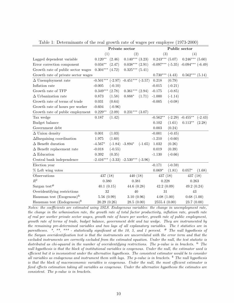
Table 1: Determinants of the real growth rate of wages per employee (1973-2000)

Private sector Public sector

(1) (2) (3) (4)

Lagged dependent variable 0.120∗∗ (2.46) 0.140∗∗∗ (3.23) 0.243∗∗∗ (5.07) 0.246∗∗∗ (5.60)

Error correction component 0.034∗∗ (2.47) 0.038∗∗∗ (2.91) -0.097∗∗∗ (-5.35) -0.094∗∗∗ (-6.49)

Growth rate of public sector wages 0.304∗∗∗ (4.72) 0.325∗∗∗ (5.41)

Growth rate of private sector wages 0.730∗∗∗ (4.43) 0.562∗∗∗ (5.14)

∆ Unemployment rate -0.501∗∗∗ (-2.97) -0.451∗∗∗ (-3.57) 0.218 (0.79)

Inflation rate -0.005 (-0.10) -0.015 (-0.21)

Growth rate of TFP 0.349∗∗∗ (2.78) 0.361∗∗∗ (2.94) -0.175 (-0.85)

∆ Urbanization rate 0.873 (1.58) 0.888∗ (1.71) -1.000 (-1.14)

Growth rate of terms of trade 0.031 (0.64) -0.005 (-0.08)

Growth rate of hours per worker -0.604 (-0.96)

Growth rate of public employment 0.229∗∗ (2.09) 0.231∗∗∗ (3.07)

Tax wedge 0.187 (1.42) -0.562∗∗ (-2.29) -0.455∗∗ (-2.43)

Budget balance 0.102 (1.61) 0.113∗∗ (2.28)

Government debt 0.003 (0.24)

∆ Union density 0.001 (1.03) -0.001 (-0.45)

∆Bargaining coordination 1.975 (1.60) -1.210 (-0.60)

∆ Benefit duration -4.567∗ (-1.84) -3.894∗ (-1.65) 1.032 (0.26)

∆ Benefit replacement rate -0.018 (-0.55) 0.019 (0.39)

∆ Education 0.392 (0.35) -1.130 (-0.66)

Central bank independence -2.416∗∗∗ (-3.33) -2.530∗∗∗ (-3.96)

Election year -0.171 (-0.59)

% Left wing votes 0.069∗ (1.81) 0.057∗ (1.68)

Observations 437 (18) 440 (18) 437 (18) 437 (18)

R2 0.380 0.381 0.228 0.263

Sargan test# 40.1 (0.15) 44.6 (0.28) 42.2 (0.09) 49.2 (0.24)

Overidentifying restrictions 32 40 31 43

Hausman test (Exogenous)& 5.56 (0.99) 3.10 (0.96) 4.08 (1.00) 0.68 (1.00)

Hausman test (Endogenous)$ 20.29 (0.26) 28.5 (0.00) 2555.4 (0.00) 23.7 (0.00)

Notes: the coefficients are estimated using 2SLS. Endogenous variables: the change in unemployment rate,the change in the urbanisation rate, the growth rate of total factor productivity, inflation rate, growth rateof real per worker private sector wages, growth rate of hours per worker, growth rate of public employment,growth rate of terms of trade, budget balance, government debt and tax wedge. They are instrumented bythe remaining pre-determined variables and two lags of all explanatory variables. The t statistics are inparentheses. *, **, *** - statistically significant at the 10, 5, and 1 percent. # The null hypothesis ofthe Sargan overidentification test is that the instruments are uncorrelated with the error term and that theexcluded instruments are correctly excluded from the estimated equation. Under the null, the test statistic isdistributed as chi-squared in the number of overidentifying restrictions. The p-value is in brackets. & Thenull hypothesis is that the block of institutional variables is exogenous. Under the null, the estimator used isefficient but it is inconsistent under the alternative hypothesis. The consistent estimator would be to considerall variables as endogenous and instrument them with lags. The p-value is in brackets. $ The null hypothesisis that the block of macroeconomic variables is exogenous. Under the null, the most efficient estimator isfixed effects estimation taking all variables as exogenous. Under the alternative hypothesis the estimates areconsistent. The p-value is in brackets.

10

which supports the idea that agents have rational expectations. Some wage stickiness is cap-

tured by the statistically significant lagged dependent variable, while there are no statistically

significant effects reported for the terms of trade or for the tax wedge.

Regarding the set of pre-determined explanatory variables (in vector Z), it is interesting

to note that the growth rate of real private sector wages is negatively affected by the index

of central bank independence. Changes in union density, bargaining coordination, the benefit

replacement rate and education do not statistically affect the growth rate of real private sector

wages. Moreover, the change in benefit duration has a negative significant coefficient.

In the estimations, the Hausman test clearly supports that the institutional variables block

is exogenous and that the variables in the macroeconomic block are endogenous. The Sargan

test points to the validity of the instruments.

3.3 Public wage determinants

We now turn to the analysis of the determinants of the growth rate of real public sector wages

per employee, which are presented in columns (3) and (4) of Table 1. The estimations pass

the Sargan test. When we include all regressors, the p-value of the test is low, albeit above

0.05. In the reduced specification the p-value is around 0.24.

The growth rate of real public sector wages per employee reacts positively to real private

sector wages, with a coefficient between 0.6 and 0.7. On the other hand, it responds negatively

to an increase in the ratio between public and private sector wages in line with our previous

conjecture. Therefore, this correction mechanism adjusts public wages downward when the

differential vis-a-vis private wages rises. Note that the absolute value of the coefficient is

roughly three times higher than the one from the similar error correction component of the

coefficient estimated in the private sector model. This means that most of the adjustment is

done via public sector wages.

The lagged dependent variable is statistically significant with a magnitude of around 0.24,

11

denoting a higher degree of wage stickiness than in the private sector. The growth of public

sector wages is not affected by any of the market variables. Regarding the explanatory fiscal

variables, improvements in the budget balance increase the growth rate of nominal public

sector wages. An increase in the budget balance ratio of 1 percentage point translates into

an increase of the growth rate of public sector wages of around 0.1 percentage points. In-

creases in the tax wedge are associated with lower public sector wage growth. In terms of

the pre-determined exogenous variables, there is a statistically significant positive effect of the

percentage votes for left wing parties.

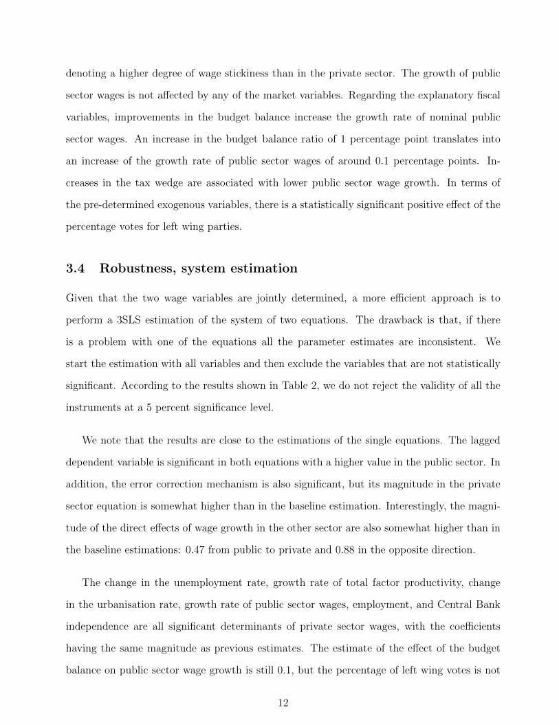
3.4 Robustness, system estimation

Given that the two wage variables are jointly determined, a more efficient approach is to

perform a 3SLS estimation of the system of two equations. The drawback is that, if there

is a problem with one of the equations all the parameter estimates are inconsistent. We

start the estimation with all variables and then exclude the variables that are not statistically

significant. According to the results shown in Table 2, we do not reject the validity of all the

instruments at a 5 percent significance level.

We note that the results are close to the estimations of the single equations. The lagged

dependent variable is significant in both equations with a higher value in the public sector. In

addition, the error correction mechanism is also significant, but its magnitude in the private

sector equation is somewhat higher than in the baseline estimation. Interestingly, the magni-

tude of the direct effects of wage growth in the other sector are also somewhat higher than in

the baseline estimations: 0.47 from public to private and 0.88 in the opposite direction.

The change in the unemployment rate, growth rate of total factor productivity, change

in the urbanisation rate, growth rate of public sector wages, employment, and Central Bank

independence are all significant determinants of private sector wages, with the coefficients

having the same magnitude as previous estimates. The estimate of the effect of the budget

balance on public sector wage growth is still 0.1, but the percentage of left wing votes is not

12

significant. The tax wedge is now statistically significant for both private and public sector. 7

Table 2: System estimation (1973-2000)

Private sector Public sector

(1) (2)

Lagged dependent variable 0.082∗∗ (2.15) 0.166∗∗∗ (4.27)

Error correction component 0.056∗∗∗ (4.66) -0.109∗∗∗ (-7.55)

Growth rate of public sector wages 0.473∗∗∗ (8.59)

Growth rate of private sector wages 0.881∗∗∗ (8.11)

∆ Unemployment rate -0.311∗∗∗ (-2.80)

Growth rate of total factor productivity 0.276∗∗∗ (2.61)

∆ Urbanization rate 1.148∗∗ (2.34) -1.572∗∗ (-2.26)

Growth rate of public employment 0.172∗∗∗ (2.59)

Tax wedge 0.208∗ (1.79) -0.404∗∗ (-2.30)

Budget balance 0.103∗∗ (2.34)

∆ Benefit duration -3.422 (-1.63)

Central bank independence -2.071∗∗∗ (-3.57)

Observations 437 (18) 437 (18)

R2 0.341 0.310

Hansen-Sargan test# 103.1 (0.057)

Notes: the coefficients are estimated using 3SLS. Endogenous variables: the change in unemployment rate,the change in the urbanisation rate, growth rate of total factor productivity, inflation rate, growth rate ofreal per worker public and private sector wages, growth rate of terms of trade, growth rate of hours perworker, change in tax wedge, the growth rate of public employment, budget balance and government debt.These endogenous variables are instrumented by the remaining pre-determined variables and two lags ofall explanatory variables. # The null hypothesis of the Hansen-Sargan overidentification test is that theinstruments are uncorrelated with the error term and that the excluded instruments are correctly excludedfrom the estimated equation. Under the null, the test statistic is distributed as chi-squared in the number ofoveridentifying restrictions (82). The p-values are in brackets.

4 Analytical framework

4.1 The model

The empirical section offered several important conclusions, useful for the setting up of the

model. First, the relation between public and private wages is bi-directional, with market

7As an alternative robustness check, we included one lag of all explanatory variables in the regressions.In general, the inclusion of lags does not carry much explanatory power. Indeed, the R-square changes verylittle from the baseline estimation, and the test that all coefficients of the lagged explanatory variables arejointly equal to zero is not rejected at the 5 percent significance level for both equations. We have alsoperformed estimations with only the subset of European Union and euro area countries, estimations with onlymacroeconomic variables and a longer sample, GMM Arellano and Bond estimation and also for the nominalwages. See Afonso and Gomes (2008).

13

forces and productivity having an effect on private sector wage growth, which is then followed

by the public sector. Second, developments in the public sector wages caused by, for instance,

political issues or by the need of fiscal tightening also affect the private sector wages. Moreover,

and in addition to the contemporaneous relation, there is also an error correction mechanism

that corrects the gap between the wages in the two sectors. Most of such correction occurs in

the public sector.

In this section we set up a dynamic labour market equilibrium model that captures the

qualitative essence of the interaction between private and public sector wage growth. The

purpose is twofold. The first objective is to uncover the transmission mechanisms of fiscal

policy through the labour market. The second is to find out if the model with only frictions

in the labour market is able to replicate the findings of the empirical section.

The model is an extension of the model by Gomes (2009a). The economy has a public

and a private sector and search and matching frictions, along the lines of Pissarides (2000).

The unemployed can only search for a job in one sector. There is some micro-econometric

evidence on the assumption of directed search between the private and public sector. Blank

(1985) finds that sectoral choice is influenced by wage comparison. Heitmueller (2006) is able

to quantify this effect and finds that an increase in 1 percent in the wages in the public sector

relative to the private sector increases the probability of choosing public sector employment

by 1.3 and 2.9 percent respectively for men and for women. The model has several differences

from the one in Gomes (2009a), that make it more realistic: it features exogenous growth in

the private sector technology; the public sector wage bill is financed through a distortionary

labour income taxation; the production function in the private sector has a more general form

with diminishing marginal returns and we analyse different fiscal rules for the setting of public

sector vacancies and wages, as opposed to discussing the optimal policy.

14

4.1.1 General setting

Public sector variables are denoted with superscript g while private sector variables are denoted

by superscript p. Time is denoted by t. The labour force consists of many individuals j ∈ [0,

1]. A proportion ut are unemployed, while the remainder are working either in the public (lgt )

or in the private (lpt ) sector

1 = lpt + lgt + ut. (4)

The presence of search and matching frictions in the labour market prevents some unemployed

individuals from finding work. The evolution of public and private sector employment depends

on the number of new matches mpt and mg

t and on separations in each sector. We consider

that, in each period, a constant fraction of jobs is destroyed, and this fraction (λ) might be

different between the two sectors

lit+1 = (1− λi)lit +mit, i = p, g. (5)

We assume that the unemployed choose in which sector they want to conduct their search, so

uit represents the number of unemployed searching in sector i. The number of matches formed

in each period is determined by two Cobb-Douglas matching functions:

mit = miui η

i

t vi 1−ηit , i = p, g. (6)

We define the share of unemployed searching for a public sector job as st =ugtut

. From the

matching functions we can define the probabilities of vacancies being filled qit, the job-finding

rates conditional on searching in a particular sector, pit, and the unconditional job-finding

rates, f it :

qit =mit

vit, pit =

mit

uit, f it =

mit

ut, i = p, g.

15

4.1.2 Households

In the presence of unemployment risk we could observe consumption differences across different

individuals. As in Merz (1995), we assume all the income of the household members is pooled

so that private consumption is equalised within the household.

The household is infinitely-lived and has preferences over the private consumption good,

ct, and a public consumption good gt

E0

∞∑t=0

βt(ln ct + ζ ln gt), (7)

where β ∈ (0, 1) is the discount factor. The budget constraint in period t is given by

ct +Bt = (1 + rt−1)Bt−1 + (1− τt)wpt lpt + (1− τt)wpt l

gt + ztut + Πt. (8)

rt−1 is the real interest rate from period t-1 to t, and Bt−1 are the holdings of one period

bonds. (1 − τt)witlit is the wage income from the members working in sector i, net of taxes,

being τ the distortinary tax rate. The unemployed members receive unemployment benefits

zt. Finally, Πt encompasses all lump sum transfers from the firm.

The household chooses consumption and bond holdings to maximize the expected lifetime

utility subject to the sequence of budget constraints, taking the public consumption good as

given. The solution is the consumption Euler equation:

1 = β(1 + rt)Et[ctct+1

]. (9)

4.1.3 Workers

The value to the household of each member depends on their current state. The value of being

employed is given by:

W it = (1− τt)wit + Etβt,t+1[(1− λi)W i

t+1 + λiUt+1], i = p, g (10)

16

where βt,t+1 = βEt[ctct+1

] is the stochastic discount factor. The value of being employed depends

on the current wage as well as on the continuation value of the job, which depends on the

separation probability in each sector. Under the assumption of directed search the agents are

either searching in the private or in the public sector. The value functions are given by

U it = zt + Etβt,t+1[p

itW

it+1 + (1− pit)Ut+1], i = p, g. (11)

The value of unemployment depends on the level of unemployment benefits and on the prob-

abilities of finding a job in the two sectors. Optimality implies the existence of movements

between the two sectors to guarantee that there is no additional gain of searching in one sector

vis-a-vis the other

Upt = U g

t = Ut. (12)

This equality determines the share of unemployed searching in each sector, and the respective

expression is implicitly given by

mptEt[W

pt+1 − Ut+1]

(1− st)=mgtEt[W

gt+1 − Ut+1]

st. (13)

The optimal search of public sector jobs increases with the number of vacancies in the public

sector and the value of a such a job, which depends positively on the public sector wages and

negatively on the separation probability.

4.1.4 Firms

The private sector representative firm hires labour to produce the private consumption good.

The production function depends on labour, but part of the resources produced have to be

used to pay for the cost of posting vacancies ςpt vpt ,

ct = apt (lp(1−α)t − ςpt v

pt ). (14)

17

The technology, apt , has a unit root and grows at an average rate on γ. Its law of motion is

given by

ln apt = ln apt−1 + γ + εat . (15)

The firm’s objective is to maximize the present discounted value of profits given by

Et

∞∑k=0

βt,t+k[apt+k(l

p(1−α)t+k − ςpt+kv

pt+k)− w

pt+kl

pt+k], (16)

and faces the law of motion for private sector employment given by

lpt+1 = (1− λp)lpt + qpt vpt . (17)

The firm takes the probability of filling a vacancy, qpt , as given. At any given point the level of

employment is predetermined and the firm can only control the number of vacancies it posts.

The solution to the problem is given by equation (18)

ςp

qpt= Etβt,t+1

at+1

at[(1− α)lp−αt+1 −

wpt+1

at+1

+ (1− λp) ςp

qpt+1

]. (18)

The optimality condition of the firm states that the expected cost of hiring a worker must

equal its expected return. The benefits of hiring an extra worker is the discounted value of

the expected difference between its marginal productivity and its wage and the continuation

value, knowing that with probability λp the match can be destroyed.

4.1.5 Private sector wage bargaining

We consider that the private sector wage is the outcome of a Nash bargaining between workers

and firms,

wpt = arg maxwp

t

(W pt − Ut)b(Jt)1−b, (19)

18

where b is the bargaining power of the unemployed and Jt is the value of the marginal job for

the firm, given by the following expression

Jt = (1− α)lp−αt − wpt + Etβt,t+1[(1− λp)Jt+1]. (20)

The Nash bargaining solution is given by:

(W pt − Ut) =

b(1− τt)1− bτt

(W pt − Ut + Jt). (21)

In the presence of distortionary taxes the share of the surplus going to the worker is lower

than its bargaining power. The reason is that for every unit that the firm gives up in favour

of the worker, the pair lose a fraction τ to the government. So they economise on their tax

payments by agreeing a lower wage.

4.1.6 Government

The government produces its consumption good using a linear technology on labour. As in

the private sector, the costs of posting vacancies are deduced from production

gt = lgt − ςgvgt . (22)

It sets a labour income tax to finance the wage bill and the unemployment benefits

τt(wpt lpt ) = (1− τt)(wgt l

gt ) + ztut, (23)

and the unemployment benefits are given by

zt = zapt . (24)

Finally, the government follows a policy for public sector vacancies and public sector wages

{vgt , wgt+1}∞t=o. We assume the government sets the wage one period in advance, at the time it

19

posts the vacancies. As st is determined based on the expected vale of both public and private

sector wage in t + 1, the current period public sector wage only affects the current level of

taxes. We assume the following rule for public sector wages:

wgt+1

wgt= Et[

wpt+1

wpt] + κ[

wgt−1wpt−1

− 1−Ψ] + εwt . (25)

In every period, the government sets its wage for the next period based on the expected

growth of private sector wages and on an error correction mechanism mimicking the public

wage premium in (3), that adjusts the differences from the actual to the target public sector

wage premium (Ψ). Public sector vacancies are set at their steady state level, designed to

target a steady state level of public sector employment

vgt = vg + εgt . (26)

Both public sector vacancies and wages are subject to shocks. We can interpret a shock to

wages (εwt ) as a short-run phenomenon coming from the need of fiscal tightness, because of

pressure from the trade union or arising from a change in government.8

4.2 Calibration

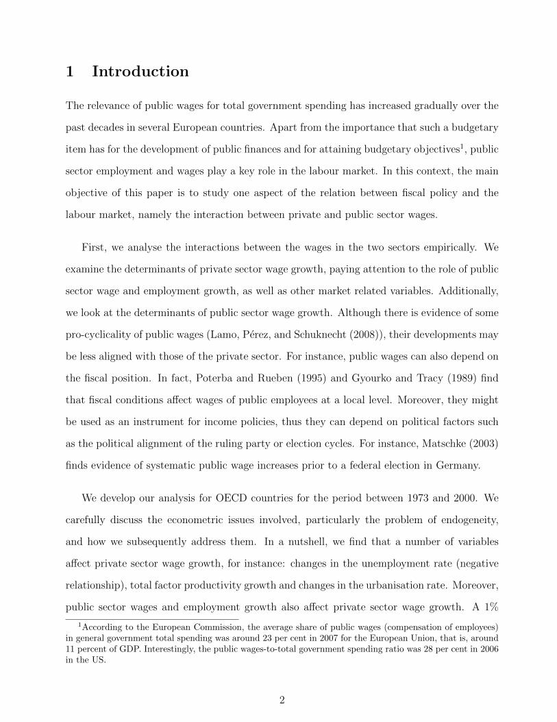
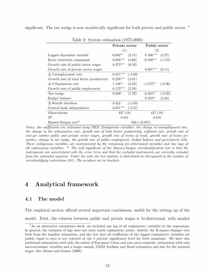
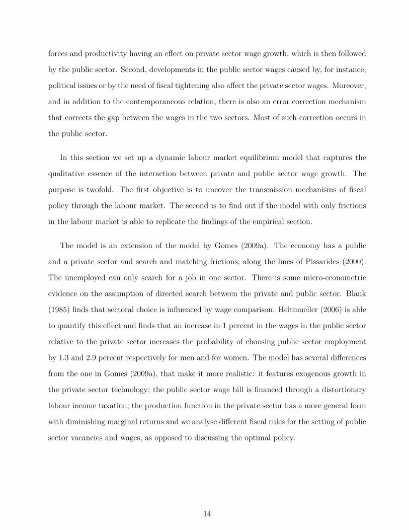
We calibrate the model at a quarterly frequency to be close to the UK economy. Figure 1

shows the level of government employment and the job-separation and job-finding rates in the

two sectors. The data are taken from the UK Labour Force Survey.9

We calibrate the steady-state public sector vacancies such that the steady-state employ-

ment in that sector is 20% of the total labour force. The separation rate in the public sector

is set to 1%, half the one in the private sector (2%). The public sector wage is set such that in

steady-state, the public sector wage premium is equal to 4%. This value is in line with several

empirical estimates (see Gregory and Borland (1999) for an overview of the literature).

8The model written in efficiency units can be found in the Appendix.9See Gomes (2009b) for a detailed study on UK labour market flows.

20

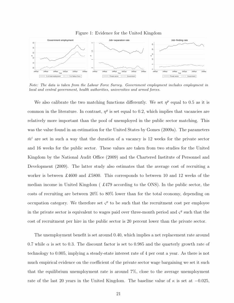
Figure 1: Evidence for the United Kingdom20

2122

2324

25

%

1993q4 1996q4 1999q4 2002q4 2005q4 2008q4Year

% of total employment % of labour force

Government employment

.51

1.5

2

%

1993q4 1996q4 1999q4 2002q4 2005q4 2008q4Year

Private sector Government

Job−separation rate

05

1015

2025

%

1993q4 1996q4 1999q4 2002q4 2005q4 2008q4Year

Private sector Government

Job−finding rate

Note: The data is taken from the Labour Force Survey. Government employment includes employment inlocal and central government, health authorities, universities and armed forces.

We also calibrate the two matching functions differently. We set ηp equal to 0.5 as it is

common in the literature. In contrast, ηg is set equal to 0.2, which implies that vacancies are

relatively more important than the pool of unemployed in the public sector matching. This

was the value found in an estimation for the United States by Gomes (2009a). The parameters

mi are set in such a way that the duration of a vacancy is 12 weeks for the private sector

and 16 weeks for the public sector. These values are taken from two studies for the United

Kingdom by the National Audit Office (2009) and the Chartered Institute of Personnel and

Development (2009). The latter study also estimates that the average cost of recruiting a

worker is between £4600 and £5800. This corresponds to between 10 and 12 weeks of the

median income in United Kingdom ( £479 according to the ONS). In the public sector, the

costs of recruiting are between 20% to 80% lower than for the total economy, depending on

occupation category. We therefore set ςp to be such that the recruitment cost per employee

in the private sector is equivalent to wages paid over three-month period and ςg such that the

cost of recruitment per hire in the public sector is 20 percent lower than the private sector.

The unemployment benefit is set around 0.40, which implies a net replacement rate around

0.7 while α is set to 0.3. The discount factor is set to 0.985 and the quarterly growth rate of

technology to 0.005, implying a steady-state interest rate of 4 per cent a year. As there is not

much empirical evidence on the coefficient of the private sector wage bargaining we set it such

that the equilibrium unemployment rate is around 7%, close to the average unemployment

rate of the last 20 years in the United Kingdom. The baseline value of κ is set at −0.025,

21

which implies an annual correction of around -0.10, the value found in the empirical section.

Much of the analysis compares the responses of the model with alternative values for the error

correction mechanism. Overall, the calibration implies a steady-state overall job-finding rate

of 0.23: 0.20 in the private and 0.03 in the public sector.

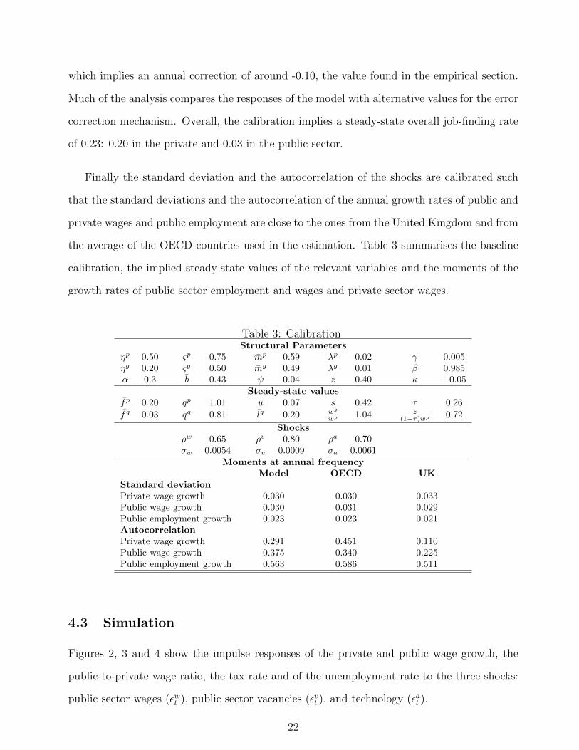
Finally the standard deviation and the autocorrelation of the shocks are calibrated such

that the standard deviations and the autocorrelation of the annual growth rates of public and

private wages and public employment are close to the ones from the United Kingdom and from

the average of the OECD countries used in the estimation. Table 3 summarises the baseline

calibration, the implied steady-state values of the relevant variables and the moments of the

growth rates of public sector employment and wages and private sector wages.

Table 3: CalibrationStructural Parameters

ηp 0.50 ςp 0.75 mp 0.59 λp 0.02 γ 0.005ηg 0.20 ςg 0.50 mg 0.49 λg 0.01 β 0.985α 0.3 b 0.43 ψ 0.04 z 0.40 κ −0.05

Steady-state valuesfp 0.20 qp 1.01 u 0.07 s 0.42 τ 0.26

fg 0.03 qg 0.81 lg 0.20 wg

wp 1.04 z(1−τ)wp 0.72

Shocksρw 0.65 ρv 0.80 ρa 0.70σw 0.0054 σv 0.0009 σa 0.0061

Moments at annual frequencyModel OECD UK

Standard deviationPrivate wage growth 0.030 0.030 0.033Public wage growth 0.030 0.031 0.029Public employment growth 0.023 0.023 0.021AutocorrelationPrivate wage growth 0.291 0.451 0.110Public wage growth 0.375 0.340 0.225Public employment growth 0.563 0.586 0.511

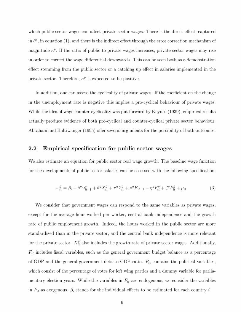
4.3 Simulation

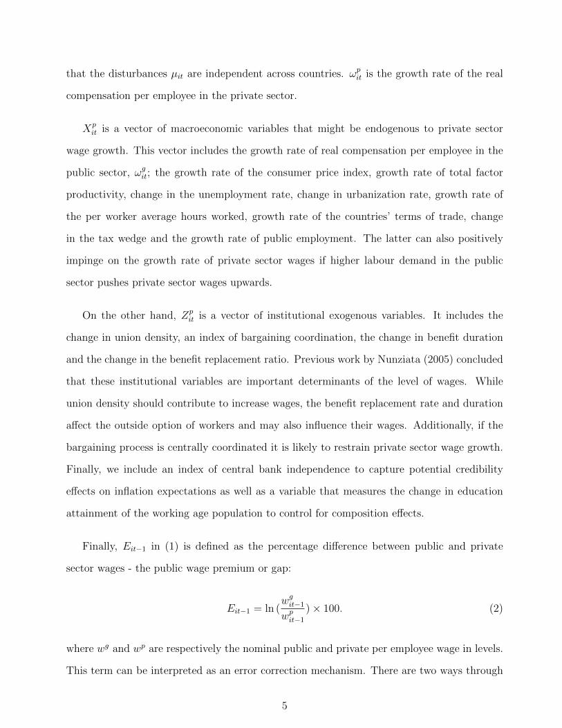
Figures 2, 3 and 4 show the impulse responses of the private and public wage growth, the

public-to-private wage ratio, the tax rate and of the unemployment rate to the three shocks:

public sector wages (εwt ), public sector vacancies (εvt ), and technology (εat ).

22

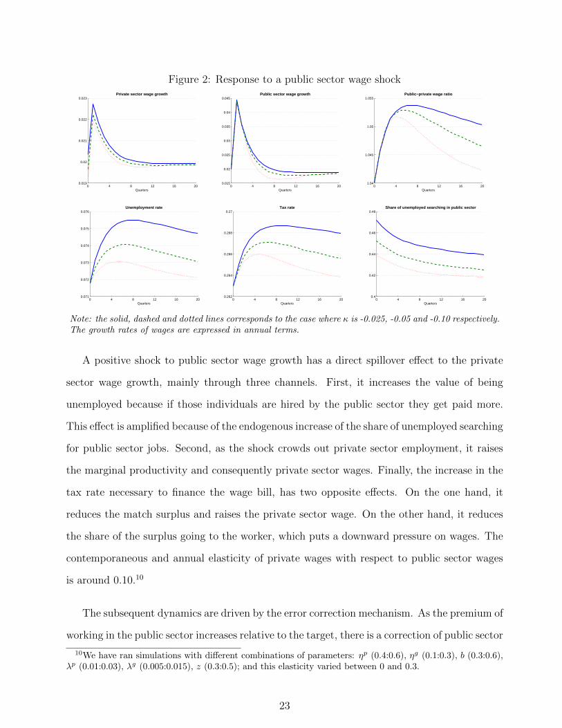
Figure 2: Response to a public sector wage shock

0 4 8 12 16 200.019

0.02

0.021

0.022

0.023Private sector wage growth

Quarters0 4 8 12 16 20

0.015

0.02

0.025

0.03

0.035

0.04

0.045Public sector wage growth

Quarters0 4 8 12 16 20

1.04

1.045

1.05

1.055Public−private wage ratio

Quarters

0 4 8 12 16 200.071

0.072

0.073

0.074

0.075

0.076Unemployment rate

Quarters0 4 8 12 16 20

0.262

0.264

0.266

0.268

0.27Tax rate

Quarters0 4 8 12 16 20

0.4

0.42

0.44

0.46

0.48Share of unemployed searching in public sector

Quarters

Note: the solid, dashed and dotted lines corresponds to the case where κ is -0.025, -0.05 and -0.10 respectively.The growth rates of wages are expressed in annual terms.

A positive shock to public sector wage growth has a direct spillover effect to the private

sector wage growth, mainly through three channels. First, it increases the value of being

unemployed because if those individuals are hired by the public sector they get paid more.

This effect is amplified because of the endogenous increase of the share of unemployed searching

for public sector jobs. Second, as the shock crowds out private sector employment, it raises

the marginal productivity and consequently private sector wages. Finally, the increase in the

tax rate necessary to finance the wage bill, has two opposite effects. On the one hand, it

reduces the match surplus and raises the private sector wage. On the other hand, it reduces

the share of the surplus going to the worker, which puts a downward pressure on wages. The

contemporaneous and annual elasticity of private wages with respect to public sector wages

is around 0.10.10

The subsequent dynamics are driven by the error correction mechanism. As the premium of

working in the public sector increases relative to the target, there is a correction of public sector

10We have ran simulations with different combinations of parameters: ηp (0.4:0.6), ηg (0.1:0.3), b (0.3:0.6),λp (0.01:0.03), λg (0.005:0.015), z (0.3:0.5); and this elasticity varied between 0 and 0.3.

23

Figure 3: Response to a public sector employment shock

0 4 8 12 16 200.018

0.02

0.022

0.024

0.026

0.028Private sector wage growth

Quarters0 4 8 12 16 20

0.019

0.02

0.021

0.022

0.023

0.024Public sector wage growth

Quarters0 4 8 12 16 20

1.038

1.0385

1.039

1.0395

1.04Public−private wage ratio

Quarters

0 4 8 12 16 200.07

0.072

0.074

0.076

0.078Unemployment rate

Quarters0 4 8 12 16 20

0.262

0.264

0.266

0.268

0.27Tax rate

Quarters0 4 8 12 16 20

0.2

0.201

0.202

0.203

0.204Public employment

Quarters

Note: the solid, dashed and dotted lines corresponds to the case where κ is -0.025, -0.05 and -0.10 respectively.The growth rates of wages are expressed in annual terms.

Figure 4: Response to a technology shock

0 4 8 12 16 200.02

0.03

0.04

0.05

0.06Private sector wage growth

Quarters0 4 8 12 16 20

0.02

0.025

0.03

0.035Public sector wage growth

Quarters0 4 8 12 16 20

1.028

1.032

1.036

1.04Public−private wage ratio

Quarters

0 4 8 12 16 200.069

0.07

0.071

0.072Unemployment rate

Quarters0 4 8 12 16 20

0.259

0.26

0.261

0.262

0.263Tax rate

Quarters0 4 8 12 16 20

0.02

0.025

0.03

0.035

0.04

0.045Productivity growth

Quarters

Note: the solid, dashed and dotted lines corresponds to the case where κ is κ is -0.025, -0.05 and -0.10respectively. The growth rates of wages and technology are expressed in annual terms.

24

wages that, after 6 quarters have a growth rate below the long-run value. This adjustment

is quicker the higher the magnitude of the error correction coefficient (κ). In addition, an

increase in the unemployment rate occurs after the shock.

A positive shock to public sector vacancies initially raises private sector wage growth (see

Figure 3). The annual elasticity is around 0.3. Both the tax and the bargaining channel

drive the wages up but, additionally, public employment crowds out the employment in the

private sector raising the average productivity of workers which serves as a reference for the

bargaining process. The increase in the private sector wages reduces the premium paid in the

public sector relative to the target, therefore, after the initial period the public sector wages

grow above the average to catch up with the private sector.

Regarding a technology shock, depicted in Figure 4, the private sector wage growth in-

creases substantially and contemporaneously, and stays above average for several periods. As

the public-private wage premium is reduced, the wages in the public sector grow at a faster

pace in the subsequent periods.

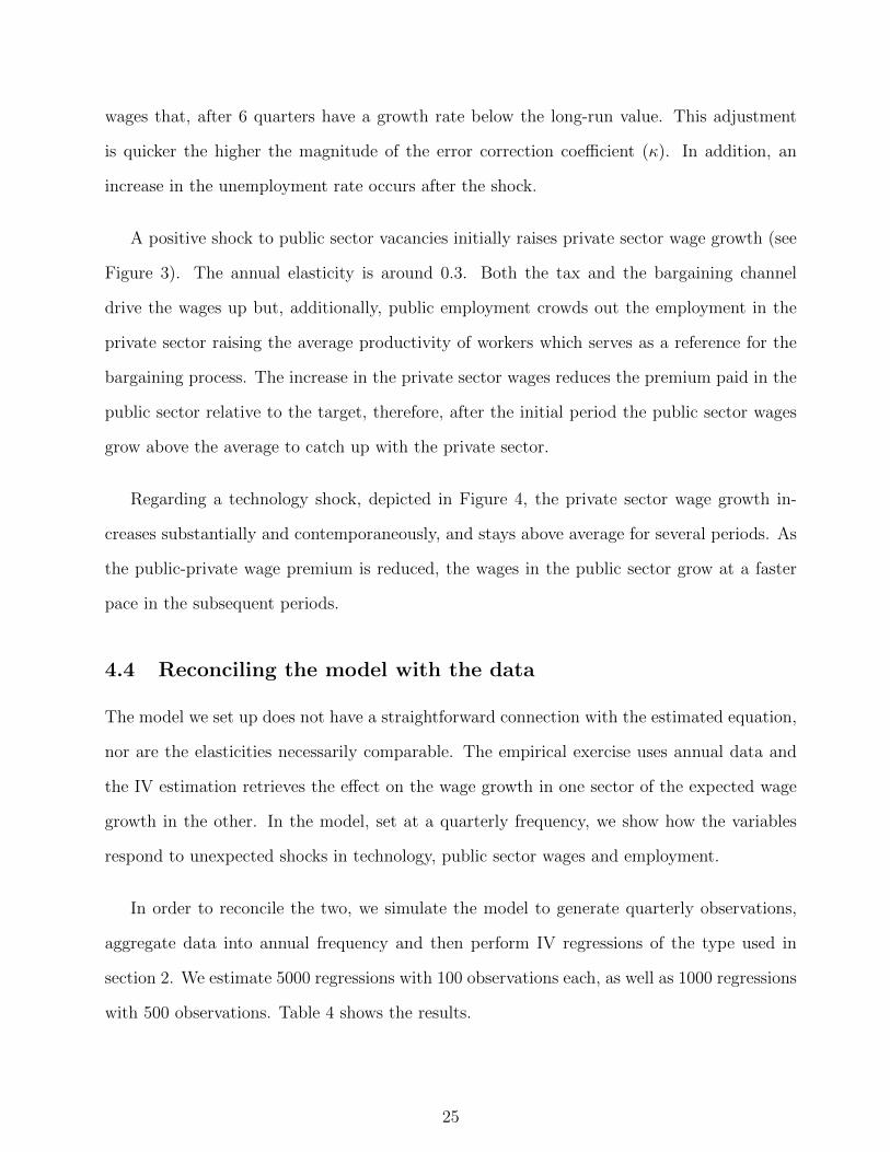
4.4 Reconciling the model with the data

The model we set up does not have a straightforward connection with the estimated equation,

nor are the elasticities necessarily comparable. The empirical exercise uses annual data and

the IV estimation retrieves the effect on the wage growth in one sector of the expected wage

growth in the other. In the model, set at a quarterly frequency, we show how the variables

respond to unexpected shocks in technology, public sector wages and employment.

In order to reconcile the two, we simulate the model to generate quarterly observations,

aggregate data into annual frequency and then perform IV regressions of the type used in

section 2. We estimate 5000 regressions with 100 observations each, as well as 1000 regressions

with 500 observations. Table 4 shows the results.

25

Table 4: IV estimation with simulated dataPrivate sector Public sector

Nobs=100 Nobs=500 Nobs=100 Nobs=500Nreg=5000 Nreg=1000 Nreg=5000 Nreg=1000

Lagged dependent variable -0.139 (0.083) -0.058 (0.059) 0.243 (0.090) 0.230 (0.045)Error correction component 0.018 (0.021) 0.016 (0.010) -0.103 (0.043) -0.075 (0.016)Growth rate of public sector wages 0.192 (0.125) 0.210 (0.073)Growth rate of private sector wages 0.697 (0.267) 0.857 (0.159)Growth rate of TFP 0.807 (0.164) 0.626 (0.111)Growth rate of public employment -0.027 (0.083) -0.051 (0.042)R2 0.867 0.801 0.294 0.199

Notes: the coefficients are estimated using 2SLS. Endogenous variables: total factor productivity, growthrate of real per worker private and public sector sector wages, growth rate of public employment. They areinstrumented by two lags of all explanatory variables. The standard deviation of the estimated coefficientsare in parentheses.

In the equation determining the public sector wage growth the three coefficients are very

close to the ones estimated for the OECD countries (see Table 1). The error correction

mechanism is between -0.08 and -0.10 and the response to expected wages is also around

0.7. Another similar feature is that the R-square of the estimation for the public sector wage

growth tends to be quite low.

In the equation determining the private sector wage growth, the coefficient of public sec-

tor wages (0.2) and the error correction mechanism (0.02), all have magnitudes similar to

the ones we estimated for the OECD countries. The coefficient of total factor productivity

growth is slightly bigger, which is expected since it is the only source of fluctuations directly

affecting private sector wages in the model. This also translates into a high R-square. The

autocorrelation coefficient is slightly negative, which means that for OECD countries there

must be some other sources of autocorrelation, perhaps wage stickiness. Still, the difference

is relatively small. On the other hand, the estimated coefficient of the growth rate of public

employment tends to be close to zero.

5 Conclusion

The purpose of this paper was to analyse the interactions between public and private sector

wages per employee in OECD countries, and to uncover the determinants of public and private

26

sector wage growth. We find that the public sector wage growth is mainly driven by private

sector wages and the government budget balance.

Regarding the private sector wage growth, we find that it is influenced by the unemploy-

ment rate, total factor productivity and urbanization rate. More important, public sector

wages and employment also affect private sector wage growth. The empirical estimates show

that a 1 percent increase in public sector wages raises the wages in the private sector by 0.3

percent, while the regressions with simulated data point to an elasticity of around 0.2 percent.

The dynamic labour market equilibrium model that we set up captures the main essence

of the interaction between public and private wages, and is quantitatively consistent with

the main estimation findings. This is true even if it abstracts from other channels that may

be relevant. For instance, higher public sector wages might translate into higher demand,

increasing the pressure on the private sector labour market. Alternatively, public sector wage

growth may also carry a signal to the private sector about the government’s expectations for

inflation. In addition, in the presence of on-the-job search, the transmission mechanism of

public sector wages can be amplified.

In light of our results, and as discussed in Pedersen et al. (1990), governments could use

their role as an employer to reduce public sector wages. This policy, in addition to reducing

the tax burden necessary to finance government spending, would have a downward impact on

private sector wages, unemployment and, possibly, on inflation. Nevertheless, one has to bear

in mind the issue of the composition of public sector employment. It is a known fact that

high-skilled workers have a negative premium from working in the public sector (Postel-Vinay

and Turon (2007)), which makes it harder for the government to recruit them (Nickell and

Quintini (2002)). Therefore, wage moderation for this group could worsen the problem and

make retention of high-skilled workers even harder in the public sector.

27

References

Abraham, K. G., and J. C. Haltiwanger (1995): “Real Wages and the Business Cycle,”

Journal of Economic Literature, 33(3), 1215–1264.

Afonso, A., and P. Gomes (2008): “Interactions between private and public sector wages,”

Working Paper Series 971, European Central Bank.

Algan, Y., P. Cahuc, and A. Zylberberg (2002): “Public employment and labour

market performance,” Economic Policy, 17(34), 7–66.

Ardagna, S. (2007): “Fiscal policy in unionized labor markets,” Journal of Economic Dy-

namics and Control, 31(5), 1498–1534.

Baker, D., A. Glyn, D. Howell, and J. Schmitt (2003): “Labor Market Institutions

and Unemployment: A Critical Assessment of the Cross-Country Evidence,” Discussion

paper.

Blank, R. M. (1985): “An analysis of workers’ choice between employment in the public

and private sectors,” Industrial and Labor Relations Review, 38(2), 211–224.

Chartered Institute of Personnel and Development (2009):

“Recruitment, retention and turnover survey report,” Available at

http://www.cipd.co.uk/subjects/recruitmen/general/.

Friberg, K. (2007): “Intersectoral wage linkages: the case of Sweden,” Empirical Economics,

32(1), 161–184.

Gomes, P. (2009a): “Fiscal policy and the labour market: the effects of public sector employ-

ment and wages,” Available at http://personal.lse.ac.uk/gomesp/1-Academia/General.htm.

(2009b): “Labour market flows: facts from the United Kingdom,” Bank of England

working papers 367.

28

Gregory, R. G., and J. Borland (1999): “Recent developments in public sector labor

markets,” in Handbook of Labor Economics, ed. by O. Ashenfelter, and D. Card, vol. 3,

chap. 53, pp. 3573–3630. Elsevier.

Gyourko, J., and J. Tracy (1989): “The Importance of Local Fiscal Conditions in Ana-

lyzing Local Labor Markets,” Journal of Political Economy, 97(5), 1208–31.

Heitmueller, A. (2006): “Public-private sector pay differentials in a devolved Scotland,”

Journal of Applied Economics, 9, 295–323.

Holmlund, B., and J. Linden (1993): “Job matching, temporary public employment, and

equilibrium unemployment,” Journal of Public Economics, 51(3), 329–343.

Jacobson, T., and H. Ohlsson (1994): “Long-Run Relations between Private and Public

Sector Wages in Sweden,” Empirical Economics, 19(3), 343–60.

Keynes, J. M. (1939): “Relative movements of real wage and output,” Economic Journal,

49(139), 34–51.

Lamo, A., J. J. Perez, and L. Schuknecht (2008): “Public and private sector wages -

co-movement and causality,” Working Paper Series 963, European Central Bank.

Matschke, X. (2003): “Are There Election Cycles in Wage Agreements? An Analysis of

German Public Employees,” Public Choice, 114(1-2), 103–35.

Merz, M. (1995): “Search in the labor market and the real business cycle,” Journal of

Monetary Economics, 36(2), 269–300.

National Audit Office (2009): “Recruiting Civil Servants efficiently,” Available at

http://www.nao.org.uk/publications/0809/recruiting civil servants effi.aspx.

Nickell, S., L. Nunziata, and W. Ochel (2005): “Unemployment in the OECD Since

the 1960s. What Do We Know?,” Economic Journal, 115(500), 1–27.

29

Nickell, S., and G. Quintini (2002): “The Consequences of The Decline in Public Sector

Pay in Britain: A Little Bit of Evidence,” Economic Journal, 112(477), F107–F118.

Nickell, W. (2006): “The CEP-OECD Institutions Data Set (1960-2004),” CEP Discussion

Papers dp0759, Centre for Economic Performance, LSE.

Nunziata, L. (2005): “Institutions and Wage Determination: a Multi-country Approach,”

Oxford Bulletin of Economics and Statistics, 67(4), 435–466.

Pissarides, C. A. (2000): Equilibrium unemployment. MIT press, 2nd edn.

Postel-Vinay, F., and H. Turon (2007): “The Public Pay Gap in Britain: Small Differ-

ences That (Don’t?) Matter,” Economic Journal, 117(523), 1460–1503.

Poterba, J. M., and K. S. Rueben (1995): “The Effect of Property-Tax Limits on Wages

and Employment in the Local Public Sector,” American Economic Review, 85(2), 384–89.

30

Appendix I - Data

Table 5: Summary statistics and sources

Mean Standarddeviation

Minimum Maximum Source

Growth rate of real private sector wages 1.42 2.17 -7.46 9.40 OECD

Growth rate of real public sector wages 1.11 3.13 -8.24 11.06 OECD

Error correction mechanism 7.78 21.26 -50.35 91.89 OECD

∆ Unemployment rate 0.09 1.07 -2.76 5.10 CEP-OECD

Total factor productivity growth rate 1.87 1.53 -2.52 6.34 OECD

∆ Urbanisation rate 0.21 0.25 -0.06 1.60 CEP

Inflation rate 5.85 4.59 0.02 23.23 OECD

Terms of Trade growth rate -0.12 4.65 -20.30 28.89 BHHS

Hours per worker growth rate -0.08 0.32 -3.82 3.15 CEP-OECD

Growth rate of public employment 1.38 2.28 -5.76 14.98 OECD

Budget Balance -2.98 4.35 -15.71 15.37 AMECO - IMF

Government Debt 54.16 28.02 2.31 140.85 AMECO - IMF

∆ Tax wedge 0.24 1.72 -10.28 5.87 BHHS

∆ Union density -0.21 1.19 -5.90 4.80 CEP

∆ Bargaining Coordination -0.01 0.08 -0.25 0.20 CEP

∆ Benefit duration 0.01 0.04 -0.21 0.32 CEP

∆ Replacement rate 0.26 3.02 -7.40 24.10 CEP

∆ Education attainment 0.08 0.09 -0.07 0.48 CEP

Central bank independence 0.53 0.21 0.17 0.93 BHHS

Election 0.30 0.46 0 1 Comparativeparties dataset

% Left wing votes 36.33 14.36 0 56 Comparativeparties dataset

Note: I use two datasets that expand the Labour Market Institutions Database created by Nickell, Nunziata, andOchel (2005): the BHHS expanded by Baker, Glyn, Howell, and Schmitt (2003) and the Center for EconomicPerformance CEP- OECD Institutions Data Set by Nickell (2006). The comparatives party dataset was createdby Duane Swank and it is available on http://www.mu.edu/polisci/Swank.htm.

Employment and wage variables

The data on public employment and wages is taken from the OECD (Economic Outlook database).

For most countries there is information on Government employment (EG). To calculate the per em-

ployee wage we divide Government final wage consumption expenditure (CGW) by Government em-

ployment. To get the wage in real terms we deflate it using the Private final consumption expenditure

deflator (PCP).

We also have the value for the Compensation of employees (WSSS) and Total employment (ET),

which refers to the total economy. We define Private sector compensation as the total Compen-

sation of employees minus the Government final wage consumption (WSSS-CGW). We define the

private employment (EP) as Total employment minus Government employment minus Self Employed

(ES): EP=ET-EG-ES. The private sector nominal wage per employee is Private sector compensation

divided by private sector employees.

31

For the case of Australia, there is no information on government employment but there is on

Private sector employment and Compensation of private sector employees. In this case, Government

employment is defined as Total employment minus Private sector employment and Compensation of

public sector employees defined as the value of Compensation of employees minus Compensation of

private sector employees.

Other variables

Benefit replacement rate - Benefit entitlement before tax as a percentage of previous earnings

before tax. Source: CEP.

Benefit duration index. Source: CEP.

Coordination index - Captures the degree of consensus between actors in collective bargaining (1

low, 3 high). Source: CEP.

Trade union density - Ratio of total reported union members (minus retired and unemployed) to

all salaried employees. Source: CEP.

Educational attainment - Average years of schooling from total population aged 15 and over

(taken from Barro and Lee dataset and intrapolated). Source: CEP.

Tax wedge - Payroll tax plus income tax plus the consumption tax rate. Source: BHHS.

Productivity growth - Growth rate of productivity per worker. Source: OECD.

Terms of trade - Growth rate of terms of trade. Source: BHHS.

Urbanisation rate - Percentage of the population living in urban areas (taken from the World

Bank World Development Indicators). Source: CEP.

Inflation - Source: OECD.

Unemployment rate - Source: CEP.

Budget Balance - Government balance as percentage of GDP. Source: AMECO European Com-

mission database, complemented with IMF data for early years.

Government debt - Government debt as percentage of GDP. Source: AMECO European Com-

mission database, complemented with IMF data for early years.

Election year - Dummy if there was a parliamentary of presidential election. Source: Comparative

parties dataset.

Left wing - Percentage of left with votes of last parliamentary elections. Source: Comparative

parties dataset.

Central Bank Independence Index. Source: BHHS

32

Appendix II - Model in efficiency units

As the technology has a unit root with drift, the model does not have a steady state. There isa balance growth path in which employment, unemployment, vacancies and labour market flows areconstant; and in which wages, consumption, the value of employment and unemployment and thevalue of a job for the firm are growing at rate γ values. We define the variables in efficiency unitswith tilde (as a ratio of technology),

wpt =wptat, wgt+1 =

wpt+1

at, ct =

ctat, W i

t =W it

at, U it =

U itat, J it =

J itat,ztat

= z,ς itat

= ς i.

We can re-write the non-stationary equations in efficiency units. The Euler equation becomes:

1 = β(1 + rt)Et[ctct+1

at+1

at]. (27)

The value functions become:

W gt = (1− τt)wgt

atat−1

+ Etβt,t+1at+1

at[(1− λg)W g

t+1 + λiUt+1], i = p, g, (28)

W pt = (1− τt)wpt + Etβt,t+1

at+1

at[(1− λp)W p

t+1 + λpUt+1], i = p, g, (29)

U it = z + Etβt,t+1at+1

at[pitW

it+1 + (1− pit)Ut+1], i = p, g, (30)

Jt = (1− α)lp−αt − wpt + Etβt,t+1at+1

at[(1− λp)Jt+1]. (31)

The first order condition from the firm and the Nash bargaining becomes

ςp

qpt= Etβt,t+1

at+1

at[(1− α)lp−αt+1 − w

pt+1 + (1− λp) ςp

qpt+1

], (32)

(W pt − Ut) =

b(1− τt)1− bτt

(W pt − Ut + Jt). (33)

Finally, the equations for the public sector become:

τt(wpt lpt ) = (1− τt)

(wgt lgt )

gat+ zut, (34)

wgt+1at

wgt at−1= Et[

apt+1

apt

wpt+1

wpt] + κ[

wgt−1wpt−1

− 1−Ψ] + εwgt , (35)

where

gat =aptapt−1

= exp(γ + εat ). (36)

33