Interaction of viscous free-surface ows with topography

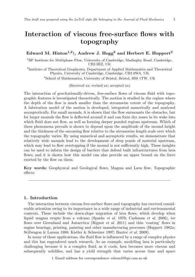
This draft was prepared using the LaTeX style file belonging to the Journal of Fluid Mechanics 1

Interaction of viscous free-surface flows withtopography

Edward M. Hinton1,2†, Andrew J. Hogg3 and Herbert E. Huppert2

1BP Institute for Multiphase Flow, University of Cambridge, Madingley Road, Cambridge,CB3 0EZ, UK

2Institute of Theoretical Geophysics, Department of Applied Mathematics and TheoreticalPhysics, University of Cambridge, Cambridge, CB3 0WA, UK

3School of Mathematics, University of Bristol, Bristol, BS8 1TW, UK

(Received xx; revised xx; accepted xx)

The interaction of gravitationally-driven, free-surface flows of viscous fluid with topo-graphic features is investigated theoretically. The motion is studied in the regime wherethe depth of the flow is much smaller than the streamwise extent of the topography.A lubrication model of the motion is developed, integrated numerically and analysedasymptotically. For small mounds, it is shown that the flow surmounts the obstacles, butfor larger mounds the flow is deflected around it and can form dry zones in its wake intowhich fluid does not flow, as well as forming deeper ponded regions upstream. Which ofthese phenomena prevails is shown to depend upon the amplitude of the mound heightand the thickness of the oncoming flow relative to the streamwise length scale over whichthe topography varies. By using numerical and asymptotic results, we demonstrate thatrelatively wide mounds lead to the development of deep ponds of material upstream,which may lead to flow overtopping if the mound is not sufficiently high. These insightscan be used to inform the design of barriers that defend built infrastructures from lavaflows; and it is shown how this model can also provide an upper bound on the forceexerted by the flow on them.

Key words: Geophysical and Geological flows, Magma and Lava flow, Topographiceffects

1. Introduction

The interaction between viscous free-surface flows and topography has received consid-erable attention owing to its importance in a wide range of industrial and environmentalcontexts. These include the down-slope migration of lava flows, which develop whenliquid magma erupts from a volcano (Sparks et al. 1976; Cashman et al. 2006), iceflows over Greenland and Antarctica (Rignot et al. 2011) and thin ‘coating’ flows inengine bearings, printing, painting and other manufacturing processes (Huppert 1982a;Stillwagon & Larson 1988; Kistler & Schweizer 1997; Baxter et al. 2009).

In many of these applications, the fluid flow is influenced by a range of complex physicsand this has engendered much research. As an example, modelling lava is particularlychallenging because it is a complex fluid; as it cools, lava becomes more viscous andsubsequently solidifies, and has a yield strength that varies across time and space

† Email address for correspondence: [email protected]

2 E. M. Hinton, A. J. Hogg and H. E. Huppert

(Sparks et al. 1976; Griffiths 2001; Takagi & Huppert 2010). Slow travelling ice is oftenmodelled as a non-Newtonian viscous fluid using a power-law model (Glenn 1955; Hutter1982), whilst in thin coating flows over small obstacles such as adhered particles, surfacetension plays a key role (Hansen 1986; Pozrikidis & Thoroddsen 1991; Blyth & Pozrikidis2006). There have also been experiments to determine the role of inertia in thin flowsover topography (Pritchard et al. 1992). Many researchers simplify the flow physics byapplying the lubrication approximation. Gaskell et al. (2004) demonstrated that this isoften a good approximation even when it does not strictly apply (for example in flowover steep topographies).

The present study is primarily motivated by how lava flows interact with topographyand how this informs the design of barriers. Lava flows can migrate into populated areasand cause significant damage to homes and infrastructure, costing millions of dollarsto local economies (Williams & Moore 1983; Barberi & Carapezza 2013). There havebeen attempts to construct barriers to divert lava flows, but these have had limitedsuccess (Colombrita 1984; Scifoni et al. 2010). Whilst there have been some numericalsimulations and laboratory studies on controlling and diverting lava flows (Fujita et al.2009; Dietterich et al. 2015), there has been little theoretical analysis of how effectivebarriers should be designed.

Kerr et al. (2006) suggested that the formation of crust at the lateral edges of adownslope lava flow confines the lava to a channel of constant width. Over a significantrange of temperatures, lava behaves as a viscoplastic fluid, with internal stresses havinga significant influence on its gravity-driven flow (see Balmforth et al. 2002). A keychallenge for creating simplified models of lava is determining which of its non-Newtonianproperties is the most important physical process in any given situation (Balmforth et al.2000).

The interaction between a lava flow and topographical variations adds an extra layerof complexity to the modelling. In order to gain insight into the role of topography, weconsider a simplified model of lava as an isothermal Newtonian fluid and since lava flowshave large length scales relative to the capillary length, we can assume surface tension isnegligible. Such viscous Newtonian flows have been studied in the absence of undulationson a horizontal plane by Huppert (1982b), and an inclined plane by Huppert (1982a)and Lister (1992), who showed that flow from a line source on an inclined plane becomessteady far behind the contact line where it advances with constant depth. These studieshave been central to improving our understanding of lava flows and they have been usedextensively.

We analyse how a steady downslope viscous flow is perturbed by topography andapply the results to inform optimal barrier construction. Larger topographical moundscan partition the flow and lead to ‘safe’ zones in their wake in which there is no fluid.Thus, along with determining the major features of the flow, a key aim of this paper isto ascertain the dimensions and strength of a barrier necessary to protect a particularlocation from a lava flow. An increased understanding of how lava flows over topographyis also critical for our ability to use volcanic deposits for paleoclimate reconstructions(Edwards et al. 2013). The present work may also be of interest in other areas, such asthe glass industry, coating flows and glacier dynamics.

The paper is structured as follows. In section 2, we adapt Lister’s governing equationfor downslope viscous flows to incorporate the influence of topographical variations. Thisintroduces dimensionless parameters that quantify the amplitude of the mound and thedepth of the oncoming flow. We focus on the steady flow from a sustained source thatdevelops at late times after the front has passed the topography and other transienteffects have diminished. In section 3 we introduce a numerical scheme to simulate this

Interactions of viscous flow with topography 3

steady problem. The results demonstrate that dry regions, in which there is no fluid, canoccur for shallow flows past sufficiently large mounds.

To provide insights to the key physics of the problem, we first consider the simpler caseof topography which varies only in the downslope direction in §4. In this case, dry regionscannot develop. Ponding, where the flow becomes much deeper than its steady upstreamdepth, occurs upstream of any locations at which the gradient of the topography pointsupwards relative to the downwards direction of gravity. We find asymptotic expressionsfor the depth in the ponded region.

In section 5, we examine flow around topography that varies in both down- and cross-slope directions and extend our asymptotic approach to the flow over and around anaxisymmetric mound. The results show good agreement with our numerical simulations,providing both a useful validation of the numerical technique and significant insight intothe dynamical controls of these flows. When the topography is everywhere coated by thefluid, there is mathematically an ‘inner region’ in which the flow is driven primarily bythe topography and the downslope component of gravity, matched to an ‘outer region’in which gradients of the hydrostatic pressure associated with the component of gravitynormal to the slope become significant. The ‘inner’ expansion breaks down with theonset of dry regions. By reintroducing the diffusive slumping terms associated with thehydrostatic pressure gradients, we calculate the extent of the flow up the mound.

Finally, in order to apply the results to the problem of barrier construction, we considera wide elliptical mound in section 6. Our asymptotic analysis can be used to determinethe mound width and height and the upstream flow depth for which lava is diverted awayfrom a downstream region. We also calculate an upper bound for the force exerted onthe mound by the pond of lava.

2. Model

We consider the flow of a fluid of constant dynamic viscosity µ down a rigid inclinedplane at an angle β to the horizontal. We denote the downslope coordinate by X, thecross-slope coordinate by Y , the normal distance above the inclined plane by Z andtime by T . A mound of height, Dm(X,Y ) (with height scale D), is added to the plane(figure 1), where the maximum value of m is 1. The thickness of the current is given byH(X,Y, T ). We assume that the fluid is sufficiently viscous that the effects of both inertiaand surface tension can be neglected (i.e. Reynolds and Bond numbers are sufficientlysmall). We further assume that the flow is predominantly parallel to the plane and hencethe pressure, P , within the fluid is hydrostatic (Batchelor 1965),

P = P0 +∆ρg[H(X,Y ) +Dm(X,Y )− Z

]cosβ, (2.1)

where ∆ρ is the density difference between the fluid and the ambient and P0 is theambient pressure, assumed constant. The fluid velocity in the X and Y directions isgiven by

U =∆ρg

2µZ(Z − 2H

)[(∂H∂X

+D∂m

∂X

)cosβ − sinβ

], (2.2)

V =∆ρg

2µZ(Z − 2H

)(∂H∂Y

+D∂m

∂Y

)cosβ, (2.3)

respectively (Lister 1992). Local mass conservation is expressed by

∂H

∂T+

∂

∂X

(∫ H

0

UdZ

)+

∂

∂Y

(∫ H

0

V dZ

)= 0. (2.4)


(a)

line so

urce

(bi)

(bii)

(ci)

(cii)

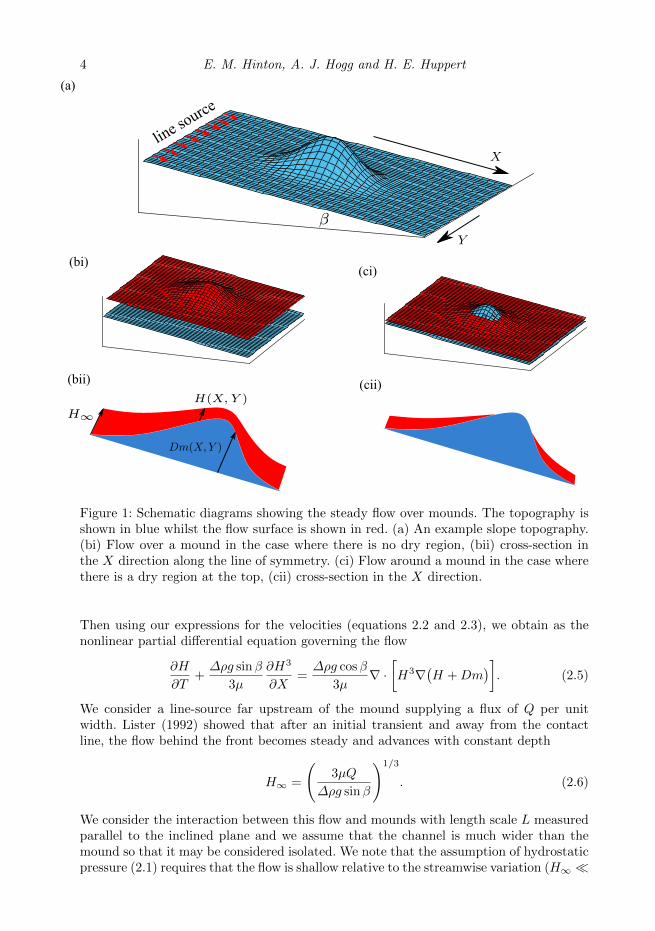
Figure 1: Schematic diagrams showing the steady flow over mounds. The topography isshown in blue whilst the flow surface is shown in red. (a) An example slope topography.(bi) Flow over a mound in the case where there is no dry region, (bii) cross-section inthe X direction along the line of symmetry. (ci) Flow around a mound in the case wherethere is a dry region at the top, (cii) cross-section in the X direction.

Then using our expressions for the velocities (equations 2.2 and 2.3), we obtain as thenonlinear partial differential equation governing the flow

∂H

∂T+∆ρg sinβ

3µ

∂H3

∂X=∆ρg cosβ

3µ∇ ·[H3∇

(H +Dm

)]. (2.5)

We consider a line-source far upstream of the mound supplying a flux of Q per unitwidth. Lister (1992) showed that after an initial transient and away from the contactline, the flow behind the front becomes steady and advances with constant depth

H∞ =

(3µQ

∆ρg sinβ

)1/3

. (2.6)

We consider the interaction between this flow and mounds with length scale L measuredparallel to the inclined plane and we assume that the channel is much wider than themound so that it may be considered isolated. We note that the assumption of hydrostaticpressure (2.1) requires that the flow is shallow relative to the streamwise variation (H∞ �


L). In terms of the parameters in the problem, the Reynolds and Bond numbers are

Re =∆ρU2/L

µU/H2∞

=H5∞∆ρ

2g

L2µ2, Bo =

∆ρgL2

γ, (2.7)

where the velocity scale is U ∼ ∆ρgH3∞/(µL) [see (2.2)] and γ is the coefficient of surface

tension.There are three length scales in the model: the mound amplitude, D; the mound’s

streamwise length scale, L; and the depth of the flow far upstream, H∞. We introducethe following dimensionless variables

x = X/L, y = Y/L, z = Z/H∞, t = QT/LH∞. (2.8)

Using equation (2.5), we find the following governing equation for the dimensionlessdepth, h(x, y, t),

∂h

∂t+∂h3

∂x= ∇ ·

[h3∇

(Fh+Mm

)], (2.9)

where

F =H∞

L tanβ=

[3µQ

(∆ρg sinβ)L3 tan3 β

]1/3(2.10)

is a dimensionless proxy for the upstream flow depth. It quantifies the importance ofthe diffusive terms on the right-hand side of equation (2.9), associated with the gravity-driven slumping of the fluid, relative to the downslope advective term on the left-handside of the same equation, associated with the gravity-driven flow down the plane. Also,

M =D

L tanβ, (2.11)

which is the ratio of the characteristic gradient of the mound, D/L, to the gradient ofthe inclined plane, tanβ. Because there are three length scales in the problem, it is fullydefined by the two dimensionless parameters, F and M.

To protect towns, barriers must be many hundreds of metres wide whilst the oncominglava flows may have a depth of the order of metres. For a typical slope gradient of 10%to 20%, we find that F � 1 and we focus our attention on this limit and investigate theeffect of varying the mound height through the parameter M.

We now describe the dimensionless mound topography, m(x, y). We begin our analysis

by assuming that the mound is axisymmetric, m = m(r), where r =√x2 + y2. The peak

dimensional height of the mound is D and we take the origin in x, y coordinates to be atthe peak of the mound, i.e. m(0) = 1. The mound height decays to zero away from theorigin (m → 0 as r → ∞). In §3 and §5, we use m = exp(−r2) but our analysis appliesto a more general class of mounds. We generalise this in §6 to analyse non-axisymmetricmounds with elliptical contours.

Since we are interested, inter alia, in determining the shape of dry regions when theyoccur, we can simplify the governing equation by restricting our attention to the steadyflow which occurs after the front of the current has passed the mound. In this case thegoverning equation is

∂h3

∂x= ∇ ·

[h3∇

(Fh+Mm

)]. (2.12)

The term on the left-hand side is associated with the component of gravity in thedownslope direction, while the right-hand side represents the motion due to the gradientsof hydrostatic pressure. The right-hand side comprises two terms: the first is due to


-2 0 2 4 6 8

0

1

2

3

0.6

0.7

0.8

0.9

1

1.1

-2 0 2 4 6 8

0

1

2

3

0.2

0.4

0.6

0.8

1

1.2

1.4

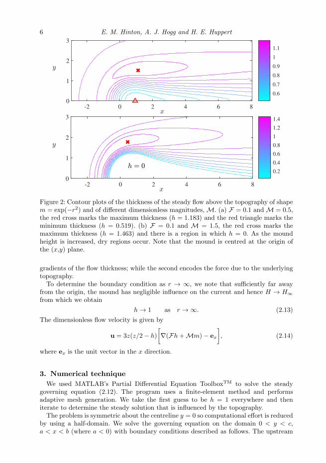
Figure 2: Contour plots of the thickness of the steady flow above the topography of shapem = exp(−r2) and of different dimensionless magnitudes,M. (a) F = 0.1 andM = 0.5,the red cross marks the maximum thickness (h = 1.183) and the red triangle marks theminimum thickness (h = 0.519). (b) F = 0.1 and M = 1.5, the red cross marks themaximum thickness (h = 1.463) and there is a region in which h = 0. As the moundheight is increased, dry regions occur. Note that the mound is centred at the origin ofthe (x,y) plane.

gradients of the flow thickness; while the second encodes the force due to the underlyingtopography.

To determine the boundary condition as r → ∞, we note that sufficiently far awayfrom the origin, the mound has negligible influence on the current and hence H → H∞from which we obtain

h→ 1 as r →∞. (2.13)

The dimensionless flow velocity is given by

u = 3z(z/2− h)

[∇(Fh+Mm)− ex

], (2.14)

where ex is the unit vector in the x direction.

3. Numerical technique

We used MATLAB’s Partial Differential Equation ToolboxTM to solve the steadygoverning equation (2.12). The program uses a finite-element method and performsadaptive mesh generation. We take the first guess to be h = 1 everywhere and theniterate to determine the steady solution that is influenced by the topography.

The problem is symmetric about the centreline y = 0 so computational effort is reducedby using a half-domain. We solve the governing equation on the domain 0 < y < c,a < x < b (where a < 0) with boundary conditions described as follows. The upstream


line source supplies constant flux so h(x = a) = 1. We allow ‘free-flow’ on the otherthree boundaries which corresponds to ∂h/∂n = 0. For each pair F , M, we run ournumerical technique on a particular domain and subsequently increase the domain sizeuntil the results become independent of further increases. For example, with F = 0.1and M = 0.5, we used a = −6, b = 26 and c = 5. A contour plot of the thickness of theflow is shown in figure 2a.

The minimum thickness of the current decreases as the mound height is increasedthrough the parameter M or as the upstream flow depth is decreased through theparameter F . For sufficiently large mounds, dry regions in which the flow depth vanishes(h = 0) can occur (see figure 2b). In the regime of very shallow upstream flow (F � 1),the critical mound height beyond which dry regions occur is Mc ≈ 1.17 for m =exp(−r2). This critical height is derived using asymptotic analysis in §5, where we alsodiscuss its physical significance.

The original numerical scheme was not effective when there were dry regions. Thediffusive term in the partial differential equation (2.12) is ∇ · (h3∇h). The nonlineardiffusion coefficient is h3, which is degenerate as h → 0. There are large gradients in hnear the dry regions and these are unable to be resolved by the numerical scheme andcan lead to spurious and inadmissible regions of h < 0.

We therefore introduced a small source upstream of the mound to provide a ‘virtual’thin film over the dry region to combat this difficulty. The governing equation is adjustedto

∂h3

∂x= ∇ ·

[h3∇

(Fh+Mm

)]+ ε(x, y), (3.1)

where ε(x, y) = ε0 exp[−(x+ 1)2 − y2]. The magnitude of the source, ε0, was minimizedsubject to the constraint that the thin film coats the dry region. The flow’s thickness iseverywhere h > 0 and the problem can be solved as described above. The edge of thedry region can be determined by analysing where the flow thickness increases from itsapproximately constant value in the thin film. For figure 2b with F = 0.1 and M = 1.5,we used ε0 = 0.008 (smaller ε0 led to regions with h < 0 in the numerical results). Wefound that doubling the source magnitude to ε0 = 0.016 increased the max depth byless than 0.1%, which demonstrates that the results from this virtual source method arehighly accurate.

The ‘dry’ region is coated in fluid owing to the ‘virtual’ source. Within the thin film of‘virtual’ fluid, the depth is approximately constant but there are large gradients in h atthe boundary of the film zone. The large gradients provide the location of the boundaryof the ‘dry’ region and we set h = 0 inside this region (see figure 2b).

We now compute the flow thickness for a wide range of two-dimensional topographies.Asymptotic analysis can help interpret the results of these computations, but beforelaunching into this analysis it is helpful to study the one-dimensional case of flow over amound which spans the channel in the y direction; m = exp(−x2) (see figure 3). Althoughdry zones are not possible in this one-dimensional problem due to the imposition of aconstant volume flus, this problem provides valuable insights into the important aspectsof the problem.


line so

urce

Figure 3: Schematic diagram showing a ‘one-dimensional’ mound topography which variesonly in the X direction.

4. Flow over one-dimensional mounds

For flow over a one-dimensional mound (as depicted in figure 3), the steady governingequation (2.12) simplifies to

dh3

dx=

d

dx

[h3(F dh

dx+Mdm

dx

)]. (4.1)

Mass conservation demands that the flow must all go over the bump and hence dryregions cannot occur, in contrast to the two-dimensional problem in which the flow maybe entirely deflected around the topography. Since the flow is steady, the downstreamflux per unit width is constant everywhere and determined by the source injection. Thiscondition can be written as∫ h

0

u(x, z) dz = h3(

1−F dh

dx−Mdm

dx

)= 1, (4.2)

where u is the flow velocity, given by the x-component of equation (2.14). The condition(4.2) cannot be satisfied if h = 0 and hence requires that h > 0 everywhere in the steadyflow over a one-dimensional mound; that is there are no dry regions possible.

We can integrate equation (4.1), or use the constant flux condition (4.2), to obtain thefollowing first order differential equation for h(x)

h3[1−Mdm

dx

]= 1 + Fh3 dh

dx. (4.3)

The numerical solution of (4.3) depends upon the shape of the mounds, given by m(x).We solve equation (4.3) together with the far-field boundary condition h→ 1 as x→ ±∞,which demands that the flow returns to its unperturbed steady-state far from the mound.In principle, we could impose the depth of the flow at some distant upstream location,h(−L) = 1, where L is positive and L � 1. However, in this case numerical integrationdownstream generates numerical instability and exponential growth in h(x). Instead, weimpose the condition at a downstream location, h(L) = 1, and then straightforwardlynumerically integrate to upstream locations, ensuring that the computed solution doesnot depend upon the magnitude of L. In figure 4 we have plotted our numerical resultsfor some shallow flows (F � 1). The numerical results exhibit a qualitative change inbehaviour as M is increased past a critical value, Mc, which will be determined below(see figure 4a where M = 0.5 and figure 4b where M = 1.5). For M > Mc, the flowdevelops a deep ‘pond’ of fluid upstream of the mound.


-2 -1 0 1 20

0.5

1

-2 -1 0 1 20

0.5

1

-5 0 50

5

10

-5 0 50

0.5

1

(a) (b)

(c) (d)

Figure 4: The profiles of the steady flow over the one-dimensional mound, m(x) =exp(−x2), as a function of streamwise distance, x. (a) Numerical solutions to equation(4.3) forM = 0.5 and two shallow oncoming flows, F = 0.1 and F = 0.02. (b) Solutionsfor a larger mound, M = 1.5. The solution is no longer independent of F to leadingorder. (c) The flow thickness relative to the height of the topography corresponding toF = 0.02 in (a). The vertical axis has been scaled so that the mound height is unity. (d)The flow thickness relative to the topography corresponding to F = 0.02 in (b). In both(c) and (d), the surface of the flow is plotted with a continuous line, while the mound isplotted with a dotted line. The fluid ‘ponds’ upstream of the mound; the flow surface ishorizontal in coordinates parallel and perpendicular to the direction of gravity (see figure5).

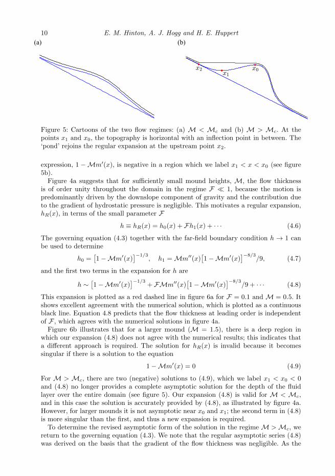
We illustrate the qualitative change in behaviour in figure 5. Increasing the moundheight beyond a critical value,Mc, leads to a region in which the topography is upslope(between x1 and x0 in figure 5b). The qualitative change in behaviour occurs at Mc

because the current cannot flow up a slope, even with a very shallow gradient, untilsufficient fluid has accumulated in a pond to overtop the highest part of the slope. This isbecause the flow is shallow and viscously controlled, with inertia playing only a negligiblerole.

The critical mound height,Mc, corresponds to a mound at which the topography firstbecomes horizontal at a single point. This can be seen by noting that the gradient of thetopography relative to gravity is given by (cf. equation 2.2)

(D/L)m′(x)− tanβ = − tanβ[1−Mm′(x)

]. (4.4)

For the case m = exp(−x2), the expression 1−Mm′(x) is strictly positive provided that

M <Mc = (e/2)1/2 ≈ 1.16 . . . (4.5)

and hence there are no regions of upslope topography in this case. For M > Mc, the


(a) (b)

Figure 5: Cartoons of the two flow regimes: (a) M < Mc and (b) M > Mc. At thepoints x1 and x0, the topography is horizontal with an inflection point in between. The‘pond’ rejoins the regular expansion at the upstream point x2.

expression, 1 −Mm′(x), is negative in a region which we label x1 < x < x0 (see figure5b).

Figure 4a suggests that for sufficiently small mound heights, M, the flow thicknessis of order unity throughout the domain in the regime F � 1, because the motion ispredominantly driven by the downslope component of gravity and the contribution dueto the gradient of hydrostatic pressure is negligible. This motivates a regular expansion,hR(x), in terms of the small parameter F

h ≡ hR(x) = h0(x) + Fh1(x) + · · · (4.6)

The governing equation (4.3) together with the far-field boundary condition h → 1 canbe used to determine

h0 =[1−Mm′(x)

]−1/3, h1 =Mm′′(x)

[1−Mm′(x)

]−8/3/9, (4.7)

and the first two terms in the expansion for h are

h ∼[1−Mm′(x)

]−1/3+ FMm′′(x)

[1−Mm′(x)

]−8/3/9 + · · · (4.8)

This expansion is plotted as a red dashed line in figure 6a for F = 0.1 and M = 0.5. Itshows excellent agreement with the numerical solution, which is plotted as a continuousblack line. Equation 4.8 predicts that the flow thickness at leading order is independentof F , which agrees with the numerical solutions in figure 4a.

Figure 6b illustrates that for a larger mound (M = 1.5), there is a deep region inwhich our expansion (4.8) does not agree with the numerical results; this indicates thata different approach is required. The solution for hR(x) is invalid because it becomessingular if there is a solution to the equation

1−Mm′(x) = 0 (4.9)

For M >Mc, there are two (negative) solutions to (4.9), which we label x1 < x0 < 0and (4.8) no longer provides a complete asymptotic solution for the depth of the fluidlayer over the entire domain (see figure 5). Our expansion (4.8) is valid for M < Mc,and in this case the solution is accurately provided by (4.8), as illustrated by figure 4a.However, for larger mounds it is not asymptotic near x0 and x1; the second term in (4.8)is more singular than the first, and thus a new expansion is required.

To determine the revised asymptotic form of the solution in the regime M >Mc, wereturn to the governing equation (4.3). We note that the regular asymptotic series (4.8)was derived on the basis that the gradient of the flow thickness was negligible. As the


-4 -3 -2 -1 0 1 2 3 40

1

2

3

4

-4 -3 -2 -1 0 1 2 3 40

0.5

1

(b)

(a)

Figure 6: The thickness of the flow as a function of streamwise distance, showing thecomparison between the numerical solutions (continuous black lines) and asymptoticapproximations found in section 4. (a) For the smaller mound regime (M = 0.5), theO(1) expansion given by equation (4.8) and plotted as a red dashed line is accurateeverywhere. (b) For a larger mound (M = 1.5), the O(1) expansion is not valid in thelarge depth region and is in fact singular here. We plot the O(F−1) expansion (equation4.18) in red dots, noting that this is valid only within the ponded region and is matchedto the regular expansion outside of this zone.

singular points of the regular series are approached (namely, x = x0 and x = x1), it isno longer the case that the gradients are negligible; instead they play a leading orderrole in the form of the solution. This motivates a different asymptotic expansion in the‘ponded’ region, close to but upstream of the peak of the mound, within which the flowis relatively thick. In the ponded region we write

h ≡ hp(x) = F−1h−1 + γ(F)h0 + · · · , (4.10)

where γ(F)� F−1 is to be determined. This form of solution is restricted to the pondedregion; far-field boundary conditions may not be applied directly and instead the solutionmust be matched to the regular series, hR(x) at ‘transition’ zones close to x = x0 andx = x2 (< x1), the latter of which is to be determined as part of the solution (see figure5).

Substituting hp(x) into (4.3) and balancing terms of the same asymptotic order, wefind that

h−1 = x−Mm(x) + c−1 and h0 = c0, (4.11)

where c−1 and c0 are constants to be determined.

First we match to the downstream form of the flow thickness by analysing the governing


equation close to x = x0. We introduce the following rescaled variables

x = x0 +(F3/X 4

)1/7η and h = (FX )

−1/7H(η), (4.12)

where X = −Mm′′(x0). The leading order terms in the governing equation in the regimeF � 1 are then given by

η =1

H3+

dH

dη. (4.13)

Matching to the downstream regular expansion (4.8), we obtain

H → η−1/3 + 19η−8/3 as η →∞. (4.14)

We note that the distinguished scalings of (4.12) are deduced by balancing the termsdownstream (4.14). Numerically integrating (4.13), we find that

H → 12η

2 + 1.611 . . . as η → −∞, (4.15)

and this condition must match the form of the solution in the ponded region. Thusevaluating (4.10) as x → x0 by substituting for x in terms of η given by (4.12), we findthat

hp ∼ F−1[x0 −Mm(x0) + c−1

]+ (FX )

−1/7η2 + γ(F)c0 + · · · . (4.16)

Matching (4.15) and (4.16), we determine that γ(F) = F−1/7 and that

c−1 = −x0 +Mm(x0) and c0 = 1.611 [−Mm′′(x0)]−1/7

. (4.17)

In the ponded region, the asymptotic expansion is given by

hp ∼ F−1[x− x0 +M(m(x0)−m(x))

]+ 1.611F−1/7

[−Mm′′(x0)

]−1/7+ · · · (4.18)

Upstream of the mound, the ponded zone re-joins a region that is modelled accuratelyby the regular expansion hR(x) around the location x = x2. We introduce a rescaledindependent variable in this zone to capture the transition in the solution between theponded and regular asymptotic series. In this case the distinguished scaling is

x = x2 + Fξ and h = h(ξ). (4.19)

In terms of these variables the leading order terms in the governing equation become

1−Mm′(x2) =1

h3+

dh

dξ. (4.20)

The matching condition upstream is that the regular series is approached and thus h→[1−Mm′(x2)]−1/3 as ξ → −∞. Substituting for x in the ponded expression (4.18) andevaluating this when ξ � 1, we find that

hp = F−1[x2 −Mm(x2) + c−1

]+ c0F−1/7 + ξ

[1−Mm′(x2)

]+ · · · . (4.21)

Thus we deduce that

x2 = x0 +M[m(x2)−m(x0)

]+ F6/71.611

[−Mm′′(x0)

]−1/7+ · · · . (4.22)

This completes the asymptotic solution for the thickness of the flowing layer in the regimeF � 1. In figure 6b we show that it captures accurately the numerically computedbehaviour for a particular parameter value.

We calculate numerically the maximum flow thickness that occurs as the fluid flowsover the mound, hm, as a function of the dimensionless amplitude of the mound,M (see


0 0.5 1 1.5 20

10

20

Figure 7: Maximum flow thickness as a function of the dimensionless amplitude of themound for F = 0.02. The numerically calculated thickness is plotted as a continuousblack line; the asymptotic prediction is plotted as a red dashed line.

figure 7), noting its weak dependence on M for values less than the critical value, Mc,but its much stronger dependence for values in excess of the critical value. This quantitymay also be evaluated directly from our asymptotic expansions for hR and hP . WhenM <Mc, the maximum depth occurs at xm(< 0) where m′′(xm) = 0 and hm = hR(xm);for m(x) = exp(−x2) this means that xm = −1/

√2 and hm = (1−M/Mc)

−1/3.When M >Mc, the maximum occurs at x = x1, since this is where dhp/dx vanishes

and so the maximum height is given by

hm = F−1{x1 − x0 −M

[m(x1)−m(x0)

]}+ c0F−1/7. (4.23)

We have found two regimes for the flow over a one-dimensional mound in the case of ashallow upstream depth (F � 1). For smaller mounds, the flow thickness is everywherecomparable to the upstream depth, but for mounds higher than a critical threshold(M > Mc), there is a region upstream of the mound in which the fluid ‘ponds’ muchdeeper than the upstream depth.

The critical dependence of the flow behaviour on the mound height will inform ourstudy of two-dimensional mounds in the next section.

5. Flow over two-dimensional mounds

The governing equation for steady flow over a mound is given by (2.12) and in thissection we analyse the motion when the mound varies both laterally and in the downslopedirection. In contrast to one-dimensional mounds (§4), the flow in this scenario need notsurmount the obstacle, but rather may be totally deflected around it. In this section weanalyse the motion in the regime F � 1 and M = O(1) in which the flowing layer ismuch shallower than both the amplitude and streamwise extent of the mound.

We follow a similar analysis as for the one-dimensional problem (§4) to determine howthe size of the mound controls the steady flow and in particular determine when theflow does not surmount the mound, leading to a dry region. Motivated by the numericalresults shown in figure 2a, we seek a regular expansion for the flow thickness for smallermounds in the form

h ≡ hR = h0 + Fh1 + · · · . (5.1)

Then, at leading order, we find the first-order partial differential equation for h0[1−M∂m

∂x

]∂h30∂x−M∂m

∂y

∂h30∂y

=Mh30∇2m. (5.2)


-4 -2 0 2 40

1

2

-4 -2 0 2 4 6 81

2

3

4

5

-4 -2 0 2 4

1

1.5

2

-4 -2 0 2 40.4

0.6

0.8

1

1.2

(ai) (aii)

(bii)

-4 -2 0 2 40

1

2(bi)

-4 -2 0 2 40

1

2(cii)(ci)

Figure 8: The asymptotic solution for flow over a two-dimensional mound, h0(x, y), inthe case that the diffusive slumping terms are neglected. The characteristics for equation(5.2) are plotted in the (x, y) plane for M = 0.5 in (ai), for M = 1.25 in (bi) andfor M = 1.5 in (ci) for four upstream cross-flow positions, yu. The characteristics areparameterised by s (see equation 5.3). The leading order flow thickness, h0(s), is plottedalong the four characteristics for M = 0.5, M = 1.25 and M = 1.5 in (aii), (bii) and(cii) respectively.

This equation neglects the diffusive slumping terms in the governing equation (2.12). Weuse the method of characteristics to find the following solution to (5.2)

dx

ds= 1−M∂m

∂x,

dy

ds= −M∂m

∂y,

d log(h30)

ds=M∇2m, (5.3)

where s parameterises the characteristics. The characteristic projections in the (x, y)plane and the flow thickness, h0(s), along some of the characteristics are plotted in figure8.

We observe that for M <Mc, dx/ds is nowhere 0, where Mc = (e/2)1/2 [see (4.5)]takes the same critical value as found for the one-dimensional mound. It correspondsto the smallest mound for which there is a point at which the topography is horizontalrelative to the direction of gravity. As in the one-dimensional problem, we anticipate


-4 -2 0 2 40

1

2

3

-4 -2 0 2 40

1

2

3

-4 -3 -2 -1 0 10

1

2

3

-4 -2 00

0.5

1

1.5

2

-4 -2 0 2 40

0.5

1

-4 -2 0 2 40

1

2

3

(ai)

(bi)

(ci)

(aii)

(bii)

(cii)

0 1 2 3 4 50

1

2

3

0 1 2 3 4 50

1

2

3

0 2 40

0.5

1

1.5(aiii)

(biii)

(ciii)

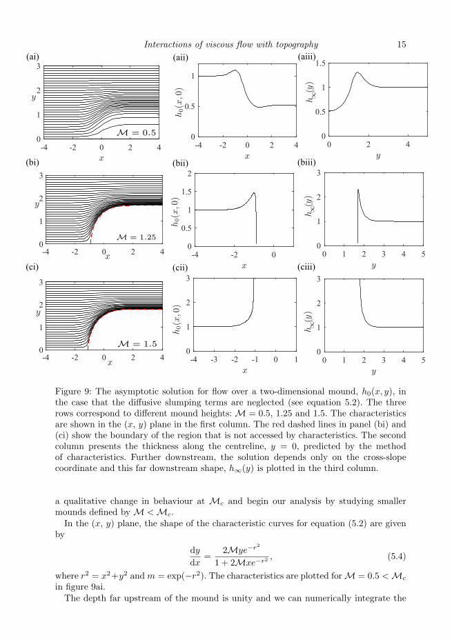
Figure 9: The asymptotic solution for flow over a two-dimensional mound, h0(x, y), inthe case that the diffusive slumping terms are neglected (see equation 5.2). The threerows correspond to different mound heights: M = 0.5, 1.25 and 1.5. The characteristicsare shown in the (x, y) plane in the first column. The red dashed lines in panel (bi) and(ci) show the boundary of the region that is not accessed by characteristics. The secondcolumn presents the thickness along the centreline, y = 0, predicted by the methodof characteristics. Further downstream, the solution depends only on the cross-slopecoordinate and this far downstream shape, h∞(y) is plotted in the third column.

a qualitative change in behaviour at Mc and begin our analysis by studying smallermounds defined by M <Mc.

In the (x, y) plane, the shape of the characteristic curves for equation (5.2) are givenby

dy

dx=

2Mye−r2

1 + 2Mxe−r2, (5.4)

where r2 = x2+y2 and m = exp(−r2). The characteristics are plotted forM = 0.5 <Mc

in figure 9ai.The depth far upstream of the mound is unity and we can numerically integrate the


0 0.2 0.4 0.6 0.8 1 1.2

0

0.5

1

Figure 10: Far downstream flow thickness over an axisymmetric mound along the line ofsymmetry (y = 0). The thickness is plotted as a function of the dimensionless moundamplitude, M, according to the leading order expansion (5.2).

system (5.3) to obtain the leading order thickness, h0. We plot a cross-section throughthe line of symmetry (y = 0) of h0 in figure 9aii.

Far downstream, the characteristic solution converges to a shape which is independentof x since dy/ds and dh/ds tend to zero; we denote

h∞(y) = limx→∞

h0(x, y). (5.5)

This far downstream shape is plotted in figure 9aiii, which illustrates that the thicknessconverges to 1 as y →∞ but not as x→∞.

The leading order thickness h0 cannot be matched with the far-field condition, h→ 1as x→∞, which suggests there is again an ‘outer’ region in which the diffusive slumpingterms are important and our current asymptotic expansion, which neglects this cross-slope spreading, is not valid (see chapter 5 of Hinch 1991). This downstream region isanalysed in subsection 5.1.

In figure 10, we plot the far downstream thickness on the line of symmetry, h∞(0), as afunction of the dimensionless mound amplitude, M. The flow thickness over the highestparts of the mound decreases as the mound amplitude increases. However, there are nodry regions for M <Mc.

Figure 10 suggests that dry regions may occur for M >Mc. For such larger mounds,dx/ds vanishes along the x axis at x1, the more negative root of equation (4.9). Thecharacteristic, which originates from (x1, ε), where ε > 0 is arbitrarily small, is plotted asa red dashed line in figure 9bi and figure 9ci. This line bounds a region that is not accessedby the characteristics. We anticipate that dry regions may occur within the area notaccessed by characteristics and this is corroborated by our numerical results (see figure2). Figure 9bii shows that the flow thickness along the centreline vanishes. This vanishingthickness is propagated along the characteristics at the edge of the inaccessible region.In figure 9cii, the behaviour is different; the flow thickness becomes singular and thissingularity is propagated along the bounding characteristics. We discuss the differencebetween these regimes later in this section.

We note that the characteristic projections (equation 5.3a and 5.3b) may be thoughtof as a phase plane. For M < Mc, there are no stationary points but for M > Mc,there are two stationary points at (x1, 0) and (x0, 0), where x1 < x0. The point (x1, 0)is at the edge of the inaccessible region and is the stationary point of interest. It is asaddle point with an unstable manifold in the y-direction and a stable manifold alongthe x axis, which can be seen in figure 9bi and figure 9ci. The point (x1, 0) is a saddlefor all M >Mc because mxx is positive here and myy is negative.


1 1.5 2 2.5 3-0.5

0

0.5

1

1.5

1 1.5 2 2.5 3-0.5

0

0.5

1

1.5(a) (b)

Figure 11: (a) Exponent k [of h0 ∼ (x1−x)k as x→ x1] as a function of the dimensionlessmound amplitude, M. (b) Exponent, k/(2 − k), of F in the flow depth (h ∼ Fk/(2−k),equation 5.17) in the ponded region upstream of the mound.

To analyse behaviour at the edge of the inaccessible region, we consider the flowthickness along the line of symmetry y = 0 as the point (x1, 0) is approached. Thecharacteristics from our asymptotic expansion, (5.1) and (5.2), indicate that the flowthickness along the centreline is given by

d log(h30)

dx=

4M(x2 − 1)e−x2

1 + 2Mxe−x2 . (5.6)

As x→ x1 the denominator tends to zero and the gradients in the flow thickness becomevery large (see figure 9bii and figure 9cii). Our asymptotic expansion breaks down here,similar to the behaviour in the one-dimensional problem (see §4).

The large x-gradients in the flow thickness, (∂h/∂x) suggest that the downslopediffusive slumping term F∂2h4/∂x2 needs to be reintroduced near the singularity. Weconsider this neighbourhood and approximate (5.6) to leading order by

d log(h30)

dx=

2(x21 − 1)

(1− 2x21)(x− x1). (5.7)

Then, according to (5.6), near x1, the leading order term, h0 is proportional to (x1−x)k,where

k =2(x21 − 1)

3(1− 2x21), (5.8)

which, through x1, is weakly dependent on M. The exponent k is plotted as a functionof M in figure 11a. The plot demonstrates that k < 2 and that k changes sign as M isincreased. Note that x1 < −1/21/2 and hence k changes sign as x1 crosses −1. In termsof M this sign change corresponds to

k >0 for M <Md = e/2 ≈ 1.36, (5.9a)

k <0 for M >Md. (5.9b)

Hence there is a change in behaviour at the secondary critical value,M =Md. This canbe observed by comparing figure 9bii, 9biii and 9cii, 9ciii; in the former,M = 1.25 <Md,whilst in the latter,M = 1.5 >Md. The regime change corresponds to a change in signof the gradient of h0 at the stagnation point, (x1, 0). The gradient is proportional to

∇2m = 4(r2 − 1)e−r2

, which changes sign (for y = 0) as x1 crosses 1.The regime change also corresponds to the inaccessible region containing the unit

circle. We deduce from (5.3) that the flow thickness, h0 is monotonically increasing


1.1 1.2 1.3 1.4 1.5 1.6 1.7 1.8 1.9 2

0

0.5

1

1.5

2

Figure 12: The downstream width of the inaccessible region, yb, as a function of thedimensionless amplitude of the mound, M, for flow over the axisymmetric mound m =exp(−r2).

along characteristics that do not pass through the unit circle, which corresponds to theregion in which the amplitude of the topography is greatest. Within the unit circle, theflow thickness is monotonically decreasing along characteristics (compare the yu = 0.01characteristics in figure 8bii and 8cii).

In figure 12, we demonstrate how the size of the inaccessible region for an exponentialmound increases with M by plotting yb, the far downstream deflection of the boundingcharacteristic [i.e. the solution of (5.3) for y(s) as s → ∞ given y(0) = ε � 1 andx(0) = x1]. For M <Md, some characteristics pass through the unit circle and henceh0 is not everywhere monotonically increasing along characteristics. We note that ybvanishes for M <Mc because the mound is sufficiently small that the flow surmountsit and is not deflected around it.

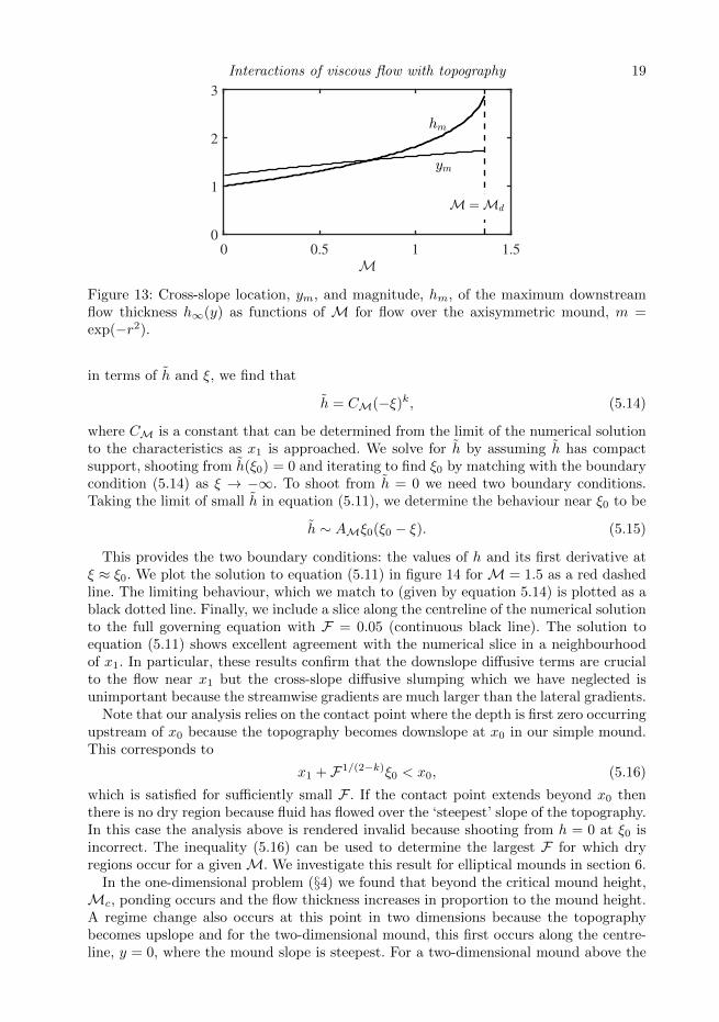
The flow thickness far downstream of the mound, h∞(y), does not vary monotonicallywith y ifM <Md, as illustrated, for example, by figure 9aiii and 9biii; instead it exhibitsa maximum, hm, which occurs at location ym [defined by h∞(ym) = hm]. The variationof hm and ym with the dimensionless mound size,M, is plotted in figure 13, noting thatforM >Md the downstream depth has become infinite at y = yb and that forM <Md

both hm and ym increase monotonically with M due to the increased flow deflectionaround the mound.

To analyse the downslope diffusive term in a neighbourhood of x1 along the symmetryaxis (y = 0), we introduce the rescalings

x = x1 + Fαξ, h = Fαkh, (5.10)

where the scaling for h is motivated by the behaviour of the characteristic solution (5.7)and (5.8). Using the governing equation (2.12), we find that along the centreline h satisfies

1

4

∂2h4

∂ξ2+AMξ

∂h3

∂ξ+BMh

3 = 0, (5.11)

where we have chosen

α = (2− k)−1, (5.12)

for a balance and

AM =M∂2m

∂x2

∣∣∣∣x=x1,y=0

, BM =M∇2m

∣∣∣∣x=x1,y=0

(5.13)

are constants. The boundary condition for (5.11) as ξ → −∞ is provided by the limitingbehaviour of the characteristic solution along the centreline, given by (5.7). Writing this


0 0.5 1 1.5

0

1

2

3

Figure 13: Cross-slope location, ym, and magnitude, hm, of the maximum downstreamflow thickness h∞(y) as functions of M for flow over the axisymmetric mound, m =exp(−r2).

in terms of h and ξ, we find that

h = CM(−ξ)k, (5.14)

where CM is a constant that can be determined from the limit of the numerical solutionto the characteristics as x1 is approached. We solve for h by assuming h has compactsupport, shooting from h(ξ0) = 0 and iterating to find ξ0 by matching with the boundarycondition (5.14) as ξ → −∞. To shoot from h = 0 we need two boundary conditions.Taking the limit of small h in equation (5.11), we determine the behaviour near ξ0 to be

h ∼ AMξ0(ξ0 − ξ). (5.15)

This provides the two boundary conditions: the values of h and its first derivative atξ ≈ ξ0. We plot the solution to equation (5.11) in figure 14 for M = 1.5 as a red dashedline. The limiting behaviour, which we match to (given by equation 5.14) is plotted as ablack dotted line. Finally, we include a slice along the centreline of the numerical solutionto the full governing equation with F = 0.05 (continuous black line). The solution toequation (5.11) shows excellent agreement with the numerical slice in a neighbourhoodof x1. In particular, these results confirm that the downslope diffusive terms are crucialto the flow near x1 but the cross-slope diffusive slumping which we have neglected isunimportant because the streamwise gradients are much larger than the lateral gradients.

Note that our analysis relies on the contact point where the depth is first zero occurringupstream of x0 because the topography becomes downslope at x0 in our simple mound.This corresponds to

x1 + F1/(2−k)ξ0 < x0, (5.16)

which is satisfied for sufficiently small F . If the contact point extends beyond x0 thenthere is no dry region because fluid has flowed over the ‘steepest’ slope of the topography.In this case the analysis above is rendered invalid because shooting from h = 0 at ξ0 isincorrect. The inequality (5.16) can be used to determine the largest F for which dryregions occur for a givenM. We investigate this result for elliptical mounds in section 6.

In the one-dimensional problem (§4) we found that beyond the critical mound height,Mc, ponding occurs and the flow thickness increases in proportion to the mound height.A regime change also occurs at this point in two dimensions because the topographybecomes upslope and for the two-dimensional mound, this first occurs along the centre-line, y = 0, where the mound slope is steepest. For a two-dimensional mound above the


-8 -6 -4 -2 0 2

0

0.5

1

1.5

Figure 14: The rescaled thickness of the fluid layer as a function of distance along the lineof symmetry (y = 0) for F = 0.05 and M = 1.5 for flow over the axisymmetric mound,m = exp(−r2). We plot the solution to (5.11) with initial condition (5.15) as a red dotteddashed line. The location of ξ0 is chosen to match with the limit of the characteristicsolution near x1, which is plotted as a dashed black line. We include a slice along thecentreline of the numerical solution from section 3, plotted as a continuous black line. Itagrees well with the solution to equation (5.11) near x1, the depth does not become zeroat ξ0 in the numerical solution because of the small virtual source.

critical height,Mc, the depth in a neighbourhood of x1 is given by the scaling in (5.10),

h ∼ Fk/(2−k). (5.17)

The exponent of F changes sign as k changes sign. It is plotted as a function of Min figure 11b. For M < Md, the exponent is positive and the depth of the flow is atmost order 1. For a larger mound (M > Md), the depth along the centreline near x1is of order Fk/(2−k), which grows as F becomes smaller. This corresponds to pondingupstream of the mound. The maximum flow thickness then occurs along y = 0, upstreamof the mound, owing to this ponding. This is in contrast to the case of M < Md (seefigure 13 and compare the two panels in figure 2). The ponding is much weaker than inthe one-dimensional case and the mound height threshold at which it occurs is higher(for example, the exponent of F is k/(2 − k) ≈ 0.04 for M = 1.5). This differenceoccurs because fluid is diverted away from the centreline and around the mound by thetopography in the cross-slope direction, whereas in the one-dimensional problem, thepond has to grow until it overcomes the mound.

The flow thickness near (x1, 0) tends to zero and we anticipate that this dry edgeis propagated by the characteristics as indicated in figure 9. Further downstream, thecharacteristics become parallel to the x axis and we anticipate that the y gradients arenon-negligible here. Thus cross-slope diffusive slumping becomes important and this actsto ‘close’ the dry region downstream, which we investigate below.

5.1. Downstream ‘outer’ region

To leading order, the regular asymptotic expansion described above converges to a fixedshape in y far downstream, i.e. h→ h∞(y) as x→∞ (see figure 9, right-hand column).Cross-channel diffusive slumping, which was neglected at leading order, smooths thisshape so that the depth converges to unity everywhere distant from the mound. Thismotivates an ‘outer’ region, in which we rescale only the downstream coordinate x to


0 5 10 15 20 25 30

0

0.2

0.4

0.6

0.8

1

0 0.5 1 1.5 2 2.5 3 3.5 4

0

0.2

0.4

0.6

0.8

1

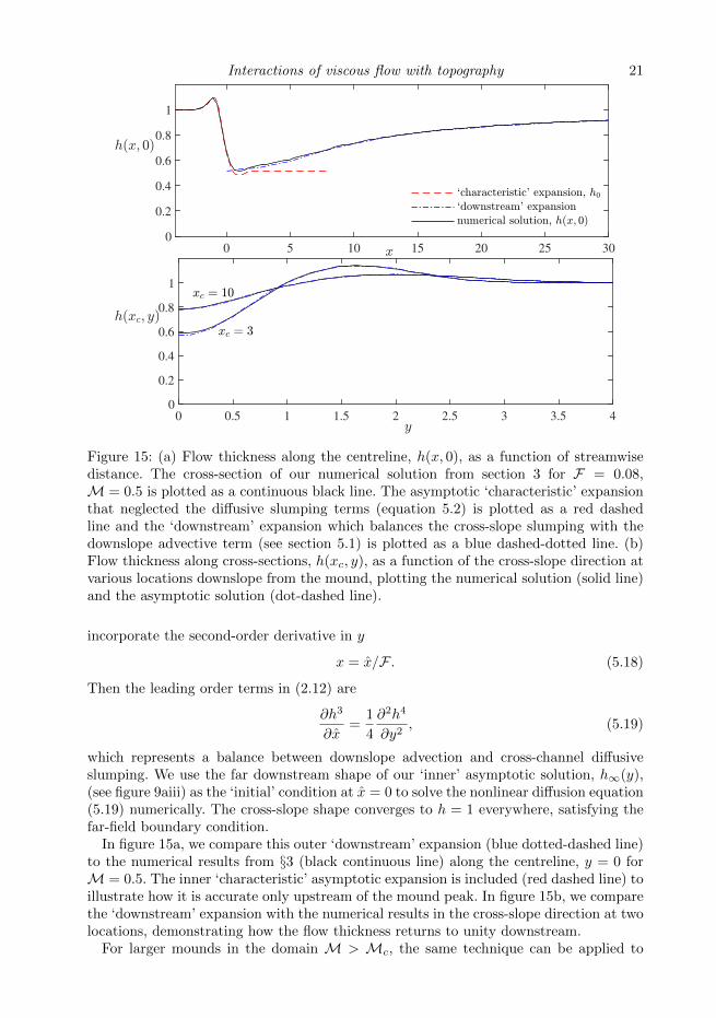
Figure 15: (a) Flow thickness along the centreline, h(x, 0), as a function of streamwisedistance. The cross-section of our numerical solution from section 3 for F = 0.08,M = 0.5 is plotted as a continuous black line. The asymptotic ‘characteristic’ expansionthat neglected the diffusive slumping terms (equation 5.2) is plotted as a red dashedline and the ‘downstream’ expansion which balances the cross-slope slumping with thedownslope advective term (see section 5.1) is plotted as a blue dashed-dotted line. (b)Flow thickness along cross-sections, h(xc, y), as a function of the cross-slope direction atvarious locations downslope from the mound, plotting the numerical solution (solid line)and the asymptotic solution (dot-dashed line).

incorporate the second-order derivative in y

x = x/F . (5.18)

Then the leading order terms in (2.12) are

∂h3

∂x=

1

4

∂2h4

∂y2, (5.19)

which represents a balance between downslope advection and cross-channel diffusiveslumping. We use the far downstream shape of our ‘inner’ asymptotic solution, h∞(y),(see figure 9aiii) as the ‘initial’ condition at x = 0 to solve the nonlinear diffusion equation(5.19) numerically. The cross-slope shape converges to h = 1 everywhere, satisfying thefar-field boundary condition.

In figure 15a, we compare this outer ‘downstream’ expansion (blue dotted-dashed line)to the numerical results from §3 (black continuous line) along the centreline, y = 0 forM = 0.5. The inner ‘characteristic’ asymptotic expansion is included (red dashed line) toillustrate how it is accurate only upstream of the mound peak. In figure 15b, we comparethe ‘downstream’ expansion with the numerical results in the cross-slope direction at twolocations, demonstrating how the flow thickness returns to unity downstream.

For larger mounds in the domain M > Mc, the same technique can be applied to


-2 -1 0 1 2 30

0.5

1

1.5

2 bounding characteristic

Figure 16: Shape of the edge of the ‘dry’ region predicted by the characteristics (reddashed line) and the shape found from our numerical simulations for three values of F ,with M = 1.5.

determine the downstream shape, but care must be taken in selecting the correct ‘initial’condition for equation (5.19). The downstream limit of the characteristic solution forM > Mc (figure 9biii and figure 9ciii) has large gradients and is not an accurateapproximation to the true depth near x = 0 because the neglected diffusive termsare significant. The shapes in figure 9biii and figure 9ciii do not provide good initialconditions. Instead, we take a y cross-section of the numerical solution at x = 0 as theinitial condition.

In figure 16, we compare the shape of the dry region predicted by the limitingcharacteristic and the shape of the dry region from the numerical results for M = 1.5and three values of F . The importance of diffusive slumping is proportional to F andhence the closing of the dry region is faster for larger F .

5.2. Summary

We have found three regimes for a shallow oncoming flow (F � 1) over an axisymmet-ric mound. For small mounds in which the slope is nowhere uphill (M <Mc), the flowgoes over and around the mound and there are no dry regions. Mounds in the secondregime, for which Mc <M <Md, give rise to dry regions. The flow thickness is order1 with respect to F because sufficient flux of the fluid flows around the mound. Forthe larger mound regime, M > Md, there is a dry region and the depth upstream ofthe mound increases as Fk/(2−k), with k < 0 [see (5.10)]. This weak dependence of thedepth on F corresponds to the signature of ponding in two dimensions. We note that ouranalysis applies to any axisymmetric mound, although Mc and Md may take differentvalues. In the next section, we consider a more general class of mound.

6. Implications for barrier design

In this section we apply our analysis to inform efforts at designing barriers to protecttowns and infrastructure from lava flows. To maximise the region downstream that isprotected whilst minimising the overall size, barriers should be wider in the cross-flowdirection than they are in the along-flow direction. This motivates considering moundswith elliptical contours; we suppose that the mound has cross-flow length scale W andalong-flow length scale L. We use the same non-dimensionalisation as in §2 and consideran elliptical Gaussian mound of profile

m(x, y) = exp[− (x2 + (y/w)2)

], (6.1)


1.25 1.3 1.35 1.4 1.45 1.5

0

0.1

0.2

0.3

Figure 17: The dimensionless upstream depth, Fc at which dry regions first occur as afunction of dimensionless mound size,M. ForM >Mc dry regions occur as the upstreamflow depth (F) tends to zero. We plot how small the flow depth must be for dry regionsto occur for different nondimensional mound widths, w. The results are obtained fromthe inequality (5.16). Wider mounds should be built taller to defend against the samedepth flow because the upstream ponding, which can overtop the mound, is enhanced.

where w = W/L is the aspect ratio of the elliptical contours of the mound. Note from(5.3) and (5.7) we deduce that this adjusts k to

k =2x21 − 1− w−2

3(1− 2x21). (6.2)

The asymptotic analysis for an axisymmetric mound from section 5 can be repeatedfor an elliptical mound. We can use the inequality (5.16) to determine how shallow theupstream flow must be for dry regions to occur. We plot the critical value of F at whicha dry region first occurs, Fc, in figure 17 for an axisymmetric mound (w = 1) and threeelliptical mounds. In the limit w → ∞, the critical line tends to Fc = 0. Thus, in thislimit, the mound is overcome by the flow, and we recover the results of §4 for flow overa one-dimensional mound.

Figure 17 demonstrates that if a mound is widened but not heightened (i.e. w isincreased andM held fixed), then the depths of flows which it defends against is reduced.In figure 18, contours of the flow thickness are plotted for F = 0.05 and M = 1.4 fordifferent mound widths, w. In figure 18a, w = 2 and there is a dry region, whilst infigure 18b w = 4 and there is no dry region. The difference arises because the pondingupstream is stronger for a wider mound. The increased ponding can overtop the mound.This effect is crucial for informing barrier construction (for example in the Mt. Etna1991-93 eruption, see Barberi & Carapezza 2013).

We illustrate the importance of ponding by considering the necessary dimensions foran example Gaussian barrier which is 200 metres wide and has a streamwise length scaleof 50 metres, on a slope with a gradient of 20%. To defend against a one metre high flow,the barrier would need to be 15 metres high. If instead the barrier was only 50 metreswide, then it would need to be about 13 metres high to provide a safe, dry region. Theseresults approximately agree with the simulations of Chirico et al. (2009), who suggestedthat barriers ought to be five to ten times the height of the average lava flow thickness.


-2 0 2 4

0

1

2

3

4

5

0.5

1

1.5

2

-2 0 2 4

0

1

2

3

4

5

0.5

1

1.5

2

2.5

Figure 18: Contour plots of the steady flow thickness above the topography in the caseof an ‘elliptical’ mound with F = 0.05 and M = 1.4. (a) w = 2; there is a dry regionwith boundary given by the contour of least thickness. (b) w = 4; for a wider mound,the ponding effect is stronger and the flow overcomes the mound (cf. figure 17). Note thedifferent scales for the thickness.

6.1. Stress on mounds

We have used our results to suggest barrier dimensions but we can also calculateestimates of the force that barriers must withstand. A major engineering concern is thatthe lava pond which can develop upstream of a barrier exerts a large force and can evenrupture the barrier (Moore 1982).

To obtain an upper bound on the force exerted by the pond, we consider a very widemound (w � 1) which is on the verge of being overtopped by the oncoming flow. Thissituation is well approximated by the flow over a one-dimensional mound in which theflow thickness is much greater upstream of the mound than over the mound. Recall (seeequation 4.18) that in the ponding region

hp ∼ F−1{x− x0 +M

[m(x0)−m(x)

]}+ · · · (6.3)

the flow surface is horizontal (perpendicular to the direction of gravity) and hencethe velocity is approximately zero (cf. equation 2.14). Therefore, the leading ordercontribution to the stress comes from the weight of the fluid in the pond. This canbe calculated by integrating the depth between x2 and x0 [where x2 is calculated from(4.22) by assuming F = 0]. The dimensional force per unit length in the downslopedirection is given by

ρgLH∞ sinβ

∫ x0

x2

hpdx = ρgL2f(M) tanβ sinβ, (6.4)

where

f(M) =M2[m(x0)2 −m(x2)2

]/2−M

∫ x0

x2

m(x)dx. (6.5)

This upper bound is independent of the upstream flow depth, H∞, because it quantifiesthe stress exerted in the case of the deepest flow which does not overtop the mound.

Consider a mound barrier with L = 50m and M = 1.5 for which f(M) ≈ 0.83. Wesuppose the oncoming lava is two and a half times as dense as water and the slope is ofgradient 0.25. With these parameters, (6.4) predicts that the maximum force per unitwidth exerted on the mound is 1.2× 107N m−1.


7. Conclusion

In this study we have investigated theoretically the interaction between a fully-developed, free-surface flow of viscous fluid down an inclined plane with topographicfeatures. Our results were derived on the basis that the flow is shallow, which in thecontext of this study requires that the flow thickness is much less than the downslopeextent of the topographic feature. In this regime, the pressure is hydrostatic to leadingorder and we computed the steady flow around and over isolated mounds. Our study wasin part motivated by the need to inform the design and dimensioning of barriers thatdeflect lava flows away from built infrastructure. Our results were computed numericallyand very often we employed asymptotic analysis to examine some of their key features.

A particular feature of our study has been the ways in which the mound causes asignificant perturbation to the oncoming flow through deflecting its passage around thebarrier, the development of ‘dry’ zones in the downslope wake of the barrier or by theestablishment of upstream, ponded regions within which the thickness of the flow isenhanced. We showed that a key discriminant of when the flow became significantlyaffected by the topography was when its gradient points upwards (i.e. ∇h.g < 0, whereg is gravitational acceleration). In such circumstances we showed for one-dimensionalobstacles, namely those that do not vary with the lateral coordinate, that the flowdevelops a pond upstream as it deepens to overtop the barrier. However, for axisymmetricmounds, the flow may be deflected around the obstacle rather than just overtoppingit, potentially leading to downslope dry zones into which the fluid does not flow. Theexistence and dimensions of the dry zones are controlled by the amplitude of the mound.Flow around non-axisymmetric mounds featured the same phenomena, although as themound became wider, the deflection of the flow was reduced, ponding was enhanced, andthe dry zone was potentially eradicated.

In future studies, it would be interesting to analyse further controls on the interactionswith topography that emerge if the flowing material exhibit some of the non-Newtonianrheology associated with lava flows. Additionally, it would be interesting to analysethe motion around tall, surface-piercing obstacles and to carry out analogue laboratoryexperiments to complement our theoretical work; this work is current underway (Hintonet al. 2019). The application of our results to field data from real lava flows is anotherarea of our concern. A key challenge is determining how the crust formation at the frontof a lava flow influences the shape of the ‘safe’ zone downstream of an obstruction.

Acknowledgements

This work was initiated at the 2018 Geophysical Fluid Dynamics summer program,Woods Hole Oceanographic Institution, which is supported by the National ScienceFoundation (award number 1332750) and the Office of Naval Research. We thank theparticipants for many helpful conversations on the porch of Walsh Cottage.

REFERENCES

Balmforth, N. J., Burbidge, A. S., Craster, R. V., Salzig, J. & Shen, A. 2000 Visco-plastic models of isothermal lava domes. Journal of Fluid Mechanics 403, 37–65.

Balmforth, N. J., Craster, R. V. & Sassi, R. 2002 Shallow viscoplastic flow on an inclinedplane. Journal of Fluid Mechanics 470, 1–29.

Barberi, F. & Carapezza, M. L. 2013 The Control of Lava Flows at Mt. Etna. AmericanGeophysical Union (AGU).

Batchelor, G. K. 1965 An introduction to fluid dynamics. Cambridge University Press.


Baxter, S. J., Power, H., Cliffe, K. A. & Hibberd, S. 2009 Three-dimensional thin filmflow over and around an obstacle on an inclined plane. Physics of Fluids 21 (3), 032102.

Blyth, M. G. & Pozrikidis, C. 2006 Film flow down an inclined plane over a three-dimensionalobstacle. Physics of Fluids 18 (5), 052104.

Cashman, K. V., Kerr, R. C. & Griffiths, R. W. 2006 A laboratory model of surfacecrust formation and disruption on lava flows through non-uniform channels. Bulletin ofVolcanology 68 (7-8), 753–770.

Chirico, G. D., Favalli, M., Papale, P., Boschi, E., Pareschi, M. T. & Mamou-Mani,A. 2009 Lava flow hazard at nyiragongo volcano, drc. Bulletin of Volcanology 71 (4),375–387.

Colombrita, R. 1984 Methodology for the construction of earth barriers to divert lava flows:the Mt. Etna 1983 eruption. Bulletin Volcanologique 47 (4), 1009–1038.

Dietterich, H. R., Cashman, K. V., Rust, A. C. & Lev, E. 2015 Diverting lava flows inthe lab. Nature Geoscience 8 (7), 494–496.

Edwards, B. R., Karson, J., Wysocki, R., Lev, E., Bindeman, I. & Kueppers, U. 2013Insights on lava–ice/snow interactions from large-scale basaltic melt experiments. Geology41 (8), 851–854.

Fujita, E., Hidaka, M., Goto, A. & Umino, S. 2009 Simulations of measures to control lavaflows. Bulletin of Volcanology 71 (4), 401–408.

Gaskell, P. H., Jimack, P. K., Sellier, M., Thompson, H. M. & Wilson, M. C. T.2004 Gravity-driven flow of continuous thin liquid films on non-porous substrates withtopography. Journal of Fluid Mechanics (509), 253–280.

Glenn, J. W. 1955 The creep of polycrystalline ice. Proceedings of the Royal Society of LondonA: Mathematical, Physical and Engineering Sciences 228 (1175), 519–538.

Griffiths, R. W. 2001 The Dynamics of Lava Flows. Annu. Rev. Fluid Mech WP01/05 (1),4–25.

Hansen, E. B. 1986 Free surface stokes flow over an obstacle. In Boundary Elements VIII , pp.783–792. Springer.

Hinch, E. J 1991 Perturbation methods.. Cambridge texts in applied mathematics . Cambridge:Cambridge University Press.

Hinton, E. M., Hogg, A. J. & Huppert, H. E. 2019 Free-surface viscous flow past cylinders.In preparation.

Huppert, H. E. 1982a Flow and instability of a viscous current down a slope. Nature300 (5891), 427–429.

Huppert, H. E. 1982b Viscous gravity currents over a rigid horizontal surface. J. Fluid Mech121.

Hutter, K. 1982 Dynamics of Glaciers pp. 245–256.

Kerr, R. C., Griffiths, R. W. & Cashman, K. V. 2006 Formation of channelized lava flowson an unconfined slope. Journal of Geophysical Research: Solid Earth 111 (10), 1–13.

Kistler, S. F. & Schweizer, P. M. 1997 Liquid film coating: scientific principles and theirtechnological implications. Springer.

Lister, J. R. 1992 Viscous flows down an inclined plane from point and line sources. Journalof Fluid Mechanics 242, 631–653.

Moore, H. J. 1982 A geologic evaluation of proposed lava diversion barriers for the noaa maunaloa observatory mauna loa volcano, hawaii. (U.S. Geol. Surv. Open-File Report 82-314 pp.1–26.

Pozrikidis, C. & Thoroddsen, S. T. 1991 The deformation of a liquid film flowing down aninclined plane wall over a small particle arrested on the wall. Physics of Fluids A: FluidDynamics 3 (11), 2546–2558.

Pritchard, W. G., Scott, L. R. & Tavener, S. J. 1992 Numerical and asymptotic methodsfor certain viscous free-surface flows. Philosophical Transactions of the Royal Society ofLondon. Series A: Physical and Engineering Sciences 340 (1656), 1–45.

Rignot, E., Mouginot, J. & Scheuchl, B. 2011 Ice flow of the antarctic ice sheet. Science333 (6048), 1427–1430.

Scifoni, S., Coltelli, M., Marsella, M., Proietti, C., Napoleoni, Q., Vicari, A. &Del Negro, C. 2010 Mitigation of lava flow invasion hazard through optimized barrier


configuration aided by numerical simulation: The case of the 2001 Etna eruption. Journalof Volcanology and Geothermal Research 192 (1-2), 16–26.

Sparks, R. S. J., Pinkerton, H. & Hulme, G. 1976 Classification and formation of lava leveeson Mount Etna, Sicily. Geology 4 (5), 269–271.

Stillwagon, L. E. & Larson, R. G. 1988 Fundamentals of topographic substrate leveling.Journal of Applied Physics 63 (11), 5251–5258.

Takagi, D. & Huppert, H. E. 2010 Initial advance of long lava flows in open channels. Journalof Volcanology and Geothermal Research 195 (2-4), 121–126.

Williams, R & Moore, J 1983 Man Against Volcano : The Eruption on Heimaey,Vestmennaeyjar, Iceland. Report USGS General Interest Publication pp. 1–26.

Interaction of viscous free-surface ows with topography

Documents

Transcript of Interaction of viscous free-surface ows with topography