Interacting Quantum Observables:Categorical Algebra and Diagrammatics

Bob Coecke1 and Ross Duncan2

1Oxford University Computing LaboratoryWolfson Building, Parks Road, Oxford OX1 3QD, UK2Laboratoire d’Information Quantique, Universite Libre de BruxellesBoulevard du Triomphe, B-1050, Bruxelles, Belgium

E-mail: 1coecke@comlab.ox.ac.uk 2rduncan@ulb.ac.be

Abstract. This paper has two tightly intertwined aims: (i) To introduce anintuitive and universal graphical calculus for multi-qubit systems, the zx-calculus,which greatly simplifies derivations in the area of quantum computation andinformation. (ii) To axiomatise complementarity of quantum observables withina general framework for physical theories in terms of dagger symmetric monoidalcategories. We also axiomatize phase shifts within this framework.

Using the well-studied canonical correspondence between graphical calculiand dagger symmetric monoidal categories, our results provide a purely graphicalformalisation of complementarity for quantum observables. Each individualobservable, represented by a commutative special dagger Frobenius algebra, givesrise to an abelian group of phase shifts, which we call the phase group. Wealso identify a strong form of complementarity, satisfied by the Z and X spinobservables, which yields a scaled variant of a bialgebra.

Contents

1 Introduction 3

2 The ZX (or green-red) graphical calculus 82.1 The ZX language: networks of wires and dots . . . . . . . . . . . . . . 82.2 The ZX equational rules . . . . . . . . . . . . . . . . . . . . . . . . . . 10

2.2.1 The T-rule. . . . . . . . . . . . . . . . . . . . . . . . . . . . . . 102.2.2 The S-rules. . . . . . . . . . . . . . . . . . . . . . . . . . . . . . 112.2.3 The B-rules. . . . . . . . . . . . . . . . . . . . . . . . . . . . . 122.2.4 The K-rules. . . . . . . . . . . . . . . . . . . . . . . . . . . . . 132.2.5 The C-rule. . . . . . . . . . . . . . . . . . . . . . . . . . . . . . 132.2.6 The D-rules. . . . . . . . . . . . . . . . . . . . . . . . . . . . . 14

2.3 Interpreting the zx-calculus in Hilbert space . . . . . . . . . . . . . . . 142.4 Universality of the zx-calculus . . . . . . . . . . . . . . . . . . . . . . 16

3 The zx-calculus in use 173.1 Adjoints and inner products . . . . . . . . . . . . . . . . . . . . . . . . 173.2 Quantum Circuits . . . . . . . . . . . . . . . . . . . . . . . . . . . . . 19

3.2.1 The ∧X gate. . . . . . . . . . . . . . . . . . . . . . . . . . . . . 193.2.2 The ∧Z gate. . . . . . . . . . . . . . . . . . . . . . . . . . . . . 20

CONTENTS 2

3.2.3 The quantum Fourier transform. . . . . . . . . . . . . . . . . . 203.3 Measurement-based quantum computing . . . . . . . . . . . . . . . . . 21

3.3.1 The teleportation protocol. . . . . . . . . . . . . . . . . . . . . 223.3.2 The state transfer protocol. . . . . . . . . . . . . . . . . . . . . 233.3.3 Multipartite states. . . . . . . . . . . . . . . . . . . . . . . . . . 243.3.4 The one-way model . . . . . . . . . . . . . . . . . . . . . . . . 25

4 Symmetric monoidal categories and graphical reasoning 274.1 Symmetric monoidal categories . . . . . . . . . . . . . . . . . . . . . . 284.2 The † functor . . . . . . . . . . . . . . . . . . . . . . . . . . . . . . . . 334.3 Diagrammatic calculus . . . . . . . . . . . . . . . . . . . . . . . . . . . 344.4 Graphical reasoning . . . . . . . . . . . . . . . . . . . . . . . . . . . . 364.5 Correctness of graphical reasoning in zx-calculus . . . . . . . . . . . . 37

5 Vector bases and state bases of observables 38

6 Algebras and observables 416.1 Monoids, comonoids, and observable structures . . . . . . . . . . . . . 416.2 Induced †-compact structure . . . . . . . . . . . . . . . . . . . . . . . 456.3 Classical points and generalised bases . . . . . . . . . . . . . . . . . . 47

7 Phase shifts and a generalised spider theorem 497.1 A monoid structure on points . . . . . . . . . . . . . . . . . . . . . . . 497.2 The decorated spider theorem . . . . . . . . . . . . . . . . . . . . . . . 517.3 Unbiased points . . . . . . . . . . . . . . . . . . . . . . . . . . . . . . . 527.4 The phase group . . . . . . . . . . . . . . . . . . . . . . . . . . . . . . 53

8 Complementarity is equivalent to the Hopf law 548.1 Observable structures with coinciding †-compact structures . . . . . . 548.2 The general case: dualisers as antipodes . . . . . . . . . . . . . . . . . 56

9 Closed complementary observable structures 579.1 Coherence for observable structures . . . . . . . . . . . . . . . . . . . . 589.2 Commutation for observable structures . . . . . . . . . . . . . . . . . . 599.3 Closedness for observable structures . . . . . . . . . . . . . . . . . . . 619.4 Our main theorem on pairs of closed observable structures . . . . . . . 63

10 Further group structure and the classical automorphisms 65

11 Deriving the zx-calculus 67

12 Non-determinism, mixed states, and classical data flow 7012.1 The CPM construction and classical concepts therein [68, 25] . . . . . 7112.2 Classicality via environment [16, 29] . . . . . . . . . . . . . . . . . . . 7312.3 Conditional diagrams [37] . . . . . . . . . . . . . . . . . . . . . . . . . 74

13 Conclusion 76

14 References 78

CONTENTS 3

1. Introduction

Quantum theory is arguably the single most successful scientific theory. While it is nowalmost a century old, many new results have been discovered by approaching quantumtheory from an computational and/or information theoretic perspective, signalling thepotential for a quantum information technology revolution. This approach has also ledto important progress in more traditional areas of physics, for example, in condensedmatter physics and statistical physics, e.g. [4], and it has provided a breath of fresh airfor quantum foundations research [45, 43, 72, 7]. Most importantly, this recent waveof progress has clearly shown that much still remains to be discovered concerning thequantum world, and how we reason about it.

Since von Neumann’s seminal book in 1932, the language in which quantum theoryis explained and is understood has been (and still is) that of Hilbert spaces. It is in thislanguage that we understand key quantum mechanical concepts such as observablesand complementarity thereof. While quantum information and computation (QIC)has proposed new concepts and paradigms to approach the quantum world, it hasnot augmented the language of quantum theory accordingly. This is in sharp contrastwith the typical practice in computer science, where new perspectives and conceptsare tightly intertwined with corresponding high-level language features. To make ablunt analogy, we can think of the Hilbert space formalism, where states mainly boildown to arrays of complex numbers, on the same footing as the arrays of 0’s and 1’sused during the stone age years of computer science. So one may wonder:

high-level languages

b1b2 . . . bn ∈ Bn' “our aim”

(c1 c2 · · · cn)T ∈ Cn

where Bn stands for strings of Booleans {0, 1} and Cn for vectors of complex numbers.A related issue is that of axiomatizing quantum theory. Despite its obvious

correctness, as a language to describe quantum theory, the Hilbert space formalismseems somewhat ad hoc from a conceptual perspective. The first to acknowledgethis was von Neumann himself, who for this reason denounced his own Hilbert spaceformalism in 1935 (see [10]), only three years after he published it. There have beenmany attempts to approach quantum theory in terms of mathematical structures otherthen Hilbert spaces [22], in the hope that this would enhance conceptual insight, butit is fair to say that none of these has provided a sufficient payoff, if any at all.

The recent advent of QIC has shed significant new light on this issue. None ofthe axiomatic approaches of the previous century provided an adequate mathematicalvehicle for the description of compound systems, even when given the description ofindividual systems. On the other hand, focussing on compoundness has producedimmense progress within QIC. This includes important foundational insights such asthe no-cloning theorem [31, 77], physical phenomena such as quantum teleportation[8], quantum algorithms such as polynomial time factoring [71], and computationalschemes such as measurement-based quantum computing [64]. Historically speaking, itwas Schrodinger who emphasised compoundness as early as 1935 [67].

In this paper we aim to catch two flies at once. We introduce a simple, intuitive,graphical high-level language, in which the atomic primitives correspond to a pair ofcomplementary observables, and we perform an axiomatic analysis of complementaritywithin the very general framework of symmetric monoidal categories (smcs). Thesetwo are related by the fact that there is a tight correspondence between graphicallanguages and smcs [47, 69], tracing back to Penrose’s work on tensor networks [61].

CONTENTS 4

The diagrammatic notation is intuitive in use, but also formally rigorous (seeSection 4), and can lead to great simplications in proofs. From a pragmatic point ofview, the graphical language provides a compact syntax for manipulating the linearoperations which are the basic elements of quantum mechanics, and it can replace morespecial purpose notations such as quantum circuits [59] or the measurement calculusfor measurement-based quantum computing [30], and unify these in one setting.

From an axiomatic point of view, monoidal categories are the most generalmathematical framework where composing systems (cf. the tensor product ‘⊗’ inthe Hilbert space framework) is a fundamental action – see [17] for a more detaileddiscussion. Since its inception in [1], formulating quantum mechanics within monoidalcategories and developing corresponding diagrammatic languages has become an activearea of research.

The bottom line is: crafting a simple intuitive graphical high-level language onthe one hand, and performing an axiomatic study which places composition of systemsat the forefront on the other hand, are in fact one and the same thing!

Our particular focus here is complementarity of quantum observables. In classicalphysics all observables are compatible: they admit sharp values at the same time. Incontrast, quantum observables are typically incompatible, and cannot be assignedsharp values simultaneously. In most axiomatic approaches incompatibility is anegative property, captured in mathematical terms by the fact that some equalityfails to hold: operators which do not commute [44], probabilities which fail to obeyKolmogorov’s axioms [63], convex sets which fail to provide a simplex structure [55, 56],and lattices which do not enjoy distributivity [11, 46].

In this paper we will take a more constructive stance and study the positivecapabilities of a pair of maximally incompatible observables, called complementary orunbiased, and show how these capabilities are exploited in QIC. Doing so will leadto an unexpected connection between quantum computation and the area of Hopfalgebrasand quantum groups [13, 50], where graphical methods have also proved to bevery fruitful [73].

All together, we obtain a rich theory from rather minimal hypotheses. Manycomputations with elementary quantum logic gates can be carried out within thistheory of interacting observables, as can many algorithms and protocols. To give onevery basic example, the fact that the composite of two ∧X-gates is the identity boilsdown to the graphical derivation:

where the dotted area is a purely graphical characterisation of complementarity.In the example above, we reasoned by rewriting : that is, by locally replacing some

part of a diagram with a diagram equal to it. This is one of the distinctive methodsof equational reasoning in graphical lanaguages. The notion of rewriting as formalmathematical tool has a long history in computer science (the text books [5] and [40]provide detailed references), and the zx-calculus introduced in this paper has indeedbeen implemented in a software tool [33, 34, 32].

Specific physical concepts give rise to specific kinds of equations over diagrams. Asthe example above shows, complementary observables introduce changes in topology,characterised by disconnecting components between the red and green dots. On theother hand, in the case of compatible observables, connected components can be

CONTENTS 5

contracted [54, 23]. The following table illustrates this: the green components aredefined in terms of one observable, and the red ones in terms of a complementary one.

compatible (self-)interaction:

complementary interaction:

For both of the depicted interactions, complementarity yields two disconnectedcomponents, while for compatible observables connectedness is preserved. Thistopological distinction has very important implications for the capabilities ofcomplementary observables in quantum informatics. The disconnectedness of thegraphical form shows the absence of information flow from one component to theother, a dynamic counterpart to the fact that knowledge of one observable in a pairof complementary observables yields no knowledge of the other observable.

We also provide an axiomatic account of phase shifts relative to an observable.This leads to the mathematical concept of a phase group. Together, our account oncomplementarity and phase groups provides a universal language for reasoning aboutmultiple two-level systems, or in modern language, qubits. For example,

HH

HH

ブ プ ベ

= HH HHブ プ ベ = ブ ベプ

is an important computation in the context of measurement based quantum computing[65], which in Hilbert space terms would involve computations with 32× 32 matrices.This example provides a straightforward translation between quantum computationalmodels, transforming a measurement-based configuration into a circuit.

From a mathematical perspective, we formalise observables in terms of algebras:Frobenius algebras, bialgebras, etc. These structures do not depend on having anunderlying Hilbert space, or indeed any linear structure whatsoever, therefore wecan study complementary observables at a much greater level of generality than theusual Hilbert space formulation of quantum mechanics. The results will apply in any‘quantum-like’ theories which bear the necessary algebraic structures. The minimalmathematical environment to support these structures is generally a dagger smc or†-smc [2, 68]. By working in an smc, we can study the central features of quantummechanics and quantum computation, without reference to Hilbert space at all. Thisresearch program was initiated by Abramsky and one of the authors in [1].

In previous work it was already established that the observables themselvescorrespond to certain commutative Frobenius algebras [27, 28]. We now explain howconceptual analysis leads to this algebraic structure, via a contrapositive of the no-cloning theorem [31, 77].

While the no-cloning theorem suggest a fundamental limitation of QIC comparedto its classical counterpart, a positive reading of it reveals that quantum states may becopied if they are known to lie in a given basis. In other words, a quantum state maybe treated as classical data, and therefore copied freely, if it is an eigenstate of a known,

CONTENTS 6

non-degenerate observable. (Throughout this paper we will treat “orthonormal basis”and “non-degenerate observable” as synonyms, and commit abuses like “measuringagainst a basis” and so on.) More concretely, given a finite dimensional Hilbert spaceH with a basis A = {|ai〉}i, the copying operation

δ : |ai〉 7→ |ai〉 ⊗ |ai〉encodes the basis A as those states that it effectively copies; the no-cloning theoremguarantees that the basis vectors are the only states with this property. Note herethat δ may be realised as a unitary map on H⊗H with one input fixed, for example,by U : |ai〉 ⊗ |aj〉 7→ |ai〉 ⊗ |ai+j〉 where the sum is taken in Zn.

Now, let ε be the linear functional on H defined by |ai〉 7→ 1 for each i. In moreconceptual terms, ε uniformly erases the elements of the basis A. Further, when ε isapplied to an output of δ we get the identity map:

(1H ⊗ ε) ◦ δ = 1H = (ε⊗ 1H) ◦ δ .In algebraic terms, ε is the co-unit for the co-multiplication δ.

Together the pair (δ, ε) form a special commutative †-Frobenius algebra on H.Previous work established the remarkable fact that every algebra of this kind on afinite dimensional Hilbert space arises as pair of copying and erasing operations forsome orthonormal basis [27, 28]. Since these algebras correspond precisely to non-degenerate quantum observables, we refer to them as observable structures. Observablestructures (δ, ε) and (δ′, ε′) which correspond to complementary observables enjoy aspecial relationship: the main body of this paper is dedicated explicating just thatrelationship, and a great deal of additional algebraic structure that follows.

Structure of this paper. This paper contains two self-contained parts, each ofwhich could be read independently of the other:

Part I. Comprising Sections 2 and 3, the first part is an informal presentation of agraphical calculus based on the interaction of complementary observables. Effectivelywe begin at the end, by presenting a calculus that demonstrates many of the key ideasof the theory, but without presenting the theory itself until Part II. It also serves tofamiliarise the reader with graphical reasoning, a tool that we will use throughout thispaper. We rely here on some familiarity with quantum computing terminology for theexamples, but no other background.

Section 2 introduces the zx-calculus , a graphical language and a set of equationalrules which are based on the Pauli Z and X spin observables, and specially tuned foruse in quantum computation. Quantum systems are represented as diagrams, andthese can be rewritten according to the equations in order to prove statements aboutthe corresponding quantum systems. This language is universal in the sense that anyoperation on n qubits can be expressed in it, as shown in Section 2.4.

In Section 3 we demonstrate a variety applications: simulating quantumcircuits, and transforming measurement-based computations into equivalent circuitsfor example. These examples are small, but the zx-calculus is appropriate for realuse, and has been used to prove non-trivial results in this area [37].

Part II. The main body of the paper, Sections 4 to 10 provide an axiomaticanalysis of complementary observables within the general framework of †-smc .Throughout, we will use graphical notation as much as possible.

From this point onwards, the Pauli Z and X spin observables will only be oneexample among all possible pairs of complementary observables. This will revealadditional properties enjoyed by the Z and X observables, as compared to other pairs

CONTENTS 7

of complementary observables. Also from this point onwards, Hilbert spaces are simplyone particular model of the axiomatic abstract algebra, and since interpretations inother models may be useful, concepts will be introduced in full generality. For example,the observables in Spekkens’ toy theory [72], are also captured by our analysis.

Section 4 reviews the necessary category theoretic background, in particular †-smcs, and their graphical notation. We rely on the work of Joyal and Street [47]and Selinger [69] to establish the validity of the graphical calculus as a rigorousmathematical syntax, and not simply a sketch.

Returning briefly to the concrete Hilbert space setting, Section 5 defines thenotions of state basis and coherent unbiased basis for Hilbert spaces, and studies theirrelation to quantum observables. These concepts play a key role in this paper, inabstract form, and to our knowledge have not appeared in the literature yet.

The technical core of the paper begins with Section 6, which provides thedefinition of observable structure—a.k.a. special commutative †-Frobenius algebra—and establishes its basic properties, including the ‘spider theorem’, giving the normalform for expressions in the language of observable structures. Before arriving at thedefinition of complementarity, in Section 7 we provide a category-theoretic accountof an important related concept, namely the phase relative to an observable. Everyobservable structure gives rise to an abelian group of phases, which behave particularlywell with respect to the normal form theorem for diagrams involving observables. Werefer to this result as the ‘decorated spider’ theorem.

In Section 8 we characterize complementarity for observable structures. InSection 9 we identify a special kind of complementary observables, which we referto as closed. These include the complementary observables that are relevant toquantum computing. We moreover provide further, equivalent, characterisations ofthese closed complementary observables. All of these equivalent characterisations takethe form of some sort of commutativity, be it either commutativity of multiplicationand a comultiplication, commutativity of a multiplication and an operation, orcommutativity of operations. These commutation properties present a remarkablecontrast with the usual characterisation of incompatibility as non-commutativity. Thetechnical development concludes in Section 10, by examining how the phase groups ofcomplementary observables act on each other to produce ‘interference’ phenomena.

Part III: Coda. Section 11 returns to the beginning by demonstrating how thegeneral theory expounded in the Part II produces the zx-calculus of Part I. We notewhich rules hold on other pairs of complementary observables, and show where theparticular features of the Z and X observables appear in the calculus.

Finally, Section 12 addresses the most obvious omission thus far; it deals withnon-determinism and classical data flow.

About this paper. The genesis of the current paper was an attempt to applyobservable structures [23, 27]—then called classical structures—to a diagrammaticnotation for measurement-based quantum computation [35]. An initial report onthese results was first presented at the icalp conference in 2008 [18], albeit undersevere space restrictions. During the intervening period the theory was under activedevelopment in Oxford, and several papers have appeared making use of the key ideasand applying them in various settings: in measurement-based quantum computation[36, 37], in the study of Spekkens’ toy theory and non-locality [19, 20], quantumprotocols [29], complementarity in the category of relations [19, 60, 41], amongothers. This paper is the first complete presentation of our categorical treatment

CONTENTS 8

of complementary observables, and it corrects several errors in the earlier paper.

2. The ZX (or green-red) graphical calculus

The state space of the elementary quantum computational unit, the qubit, is denotedby Q := C2. The vectors of the computational basis or Z-basis, are written |0〉 , |1〉,while those of the X-basis are written

|+〉 =1√2

(|0〉+ |1〉) , |−〉 =1√2

(|0〉 − |1〉) .

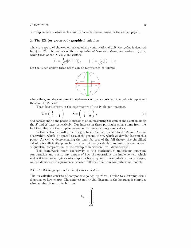
On the Bloch sphere these bases can be represented as follows:

where the green dots represent the elements of the X-basis and the red dots representthose of the Z-basis.

These bases consist of the eigenvectors of the Pauli spin matrices,

Z =

(1 00 −1

)X =

(0 11 0

), (1)

and correspond to the possible outcomes upon measuring the spin of the electron alongthe Z and X axes respectively. Our interest in these particular spins stems from thefact that they are the simplest example of complementary observables.

In this section we will present a graphical calculus, specific to the Z- and X-spinobservables, which is a special case of the general theory which we develop later in thispaper. As well as demonstrating the main features of the full theory, this simplifiedcalculus is sufficiently powerful to carry out many calculations useful in the contextof quantum computation, as the examples in Section 3 will demonstrate.

This framework refers exclusively to the mathematics underlying quantumcomputation and not to any details of how the operations are implemented, whichmakes it ideal for unifying various approaches to quantum computation. For example,we can demonstrate equivalence between different quantum computational models.

2.1. The ZX language: networks of wires and dots

The zx-calculus consists of components joined by wires, similar to electronic ciruitdiagrams or flow charts. The simplest non-trivial diagram in the language is simply awire running from top to bottom:

1Q =

in

out

CONTENTS 9

We think of diagrams as being enclosed in a box with a certain number of pointsthrough which wires enter and leave; that is, each diagram has a fixed interface.Exactly one wire must be present at each point of the interface, and we mustdistinguish which wire is connected to which point. Indeed, this is the only differencebetween the two diagrams below.

1Q⊗Q =

in1

out1

in2

out2

σQ =

in1

out1

in2

out2

It is not important whether crossing wires pass over or under (i.e. we are in a symmetricsetting, not a braided one [48]). Wires may bend, linking two outputs to form a cap,or two inputs to form a cup.

ηQ =

out1out

2

εQ =

in1in

2

From here on, the inputs and outputs will not be named, and are distinguished simplyby their ordering from left to right. We write D : m→ n to indicate that the diagramD has m inputs and n outputs.

Aside from wires, the zx-calculus contains four kinds of component:

• Z vertices (green dots), labelled by an angle α ∈ [0, 2π), called the phase. Thesecan have any number of inputs or outputs (including none).

• X vertices (red dots), labelled by a phase. These too can have any number ofinputs or outputs (including none).

• H vertices (yellow squares). These must have exactly one input and one output.

•√D vertices (black diamonds). These may not have any inputs nor any outputs.

Znm(α) =

n︷ ︸︸ ︷ブ︸ ︷︷ ︸m

Xnm(α) =

n︷ ︸︸ ︷ブ︸ ︷︷ ︸m

H = H

√D =

We refer to the Z and X vertices as “spiders”, and make the convention that if α = 0the angle is omitted.

Diagrams are built from these generators—straight, crossing, and bending wires,and Z, X, H, and

√D vertices—in two manners.

• Placing them side-by-side:

ブ

Notation: Given D : m → n and D′ : m′ → n′ their tensor product is denotedD⊗D′ : m+m′ → n+ n′.

• Connecting outputs to inputs:

CONTENTS 10

ブプπ

Notation: Given D1 : m → n and D2 : n → k their composition is denotedD2 ◦D1 : m→ k.

Therefore the terms of graphical ZX lanaguage are networks of vertices of each type,straight, crossing, and bent wires:

H

H

.

In such a network, there can be no “loose wires”: every wire must terminate at avertex, or else be an input or output.

Important examples are those spiders with 2 inputs and 1 output (cf. a binaryoperation), with no input and 1 output (cf. initiation of a value) which we will calla point, with 1 input and 2 outputs (cf. copying) and with 1 input and no output(cf. erasing):

As we will see shortly, these unlabelled spiders play a special role in the calculus, asdo those labelled by π.

2.2. The ZX equational rules

In addition to the rules for constructing diagrams, the calculus consists of a set ofequations which specify how one diagram may be transformed into another. Theserules are presented in Figure 1. We now expand on these rules and give some examplesof their use.

2.2.1. The T-rule. The informally stated T-rule will be made more precise inSection 4.3–4.5. For practical purposes, the intuitive reading of “only the topologymatters” suffices: the wires of the diagram may be arbitrarily stretched, bent,twisted, tied in knots, etc., without altering the meaning of the diagram, provided theconnections are maintained. More precisely, after identifying (e.g. by enumerating)the inputs and the outputs, any topological deformation of the internal structure ofthe network yields a network that is equal to the given one.

Two important examples of such ‘homotopic rewrites’ are:

(T1) (T2) .

In fact, these two rules can also be seen as consequences of the S-rules, whenintroducing a green dot on the caps and cups as in (S2); see Example 2.4 below.The reason for considering them within the T-rule will become clear in Section 4.5.

CONTENTS 11

“Only the topology matters” (T)

ブ

プブ+プ

ブ

プブ+プ (S1)

(S2)

(B1) (B2)

ππ π

. . . . . .

ππ π

. . . . . .

(K1)π

πブ-ブ π

πブ-ブ

(K2)

ブ = α

H H H H

H H H H

(C)

= (D1) (D2)

Figure 1. Rules for the zx-calculus

Remark 2.1. Since wires can be stretched without consequence, adding a straightlength of wire to the input or output of diagram has strictly no effect. Hence bundlesof straight wires act as identity elements in the algebra of diagrams.

Remark 2.2. While the slogan says “only the topology matters”, this does not implythat the topology is always preserved. The other rules may change the topology ofthe diagram in various ways, for example to remove loops, or to disconnect previouslyconnected vertices.

2.2.2. The S-rules. The “spider” rules govern how dots of the same colour interact.Rule (S1) states that connected dots of the same color can be merged, summing thephases; conversely, a dot can be ‘decomposed’ along one or more connecting wires.Notice that the number of connecting wires is irrelevant.

The equations (S2) specify when spiders are trivial: dots of degree 2 with phaseα = 0 can be removed, or conversely, introduced.

Example 2.3. If we view the dot Z21 : 2→ 1 as a binary operation, (S1) tells us that

it is associative:

(S1)=

(S1)= .

Less obviously, (S1) implies that this operation is commutative:

CONTENTS 12

(S1)=

(T)=

(S1)= .

We leave the reader the (easy!) exercise of showing that Z01 is a unit for this operation,

and hence that we have a commutative monoid.‡Example 2.4. The (T2) rule can be derived using the S-rules:

(S2)=

(S1)=

(S2)=

The (T1) rule is derived similarly.

Mathematically, the two S-rules state that each family of coloured dots forms aspecial commutative dagger-Frobenius algebra, equipped with a phase group. This willbe elaborated upon in Sections 6 and 7.

2.2.3. The B-rules. The B1-rule can be read loosely as “green copies red points”and “red copies green points”, in both cases “up to a diamond”.

The B2-rule is a powerful commutation principle, and generates a whole familyof equations, allowing alternating cycles of red and green dots to be replaced withsimpler graphs; see [36].

Example 2.5. An important equation derivable from the B-rules is the following:

= (B′)

This equation is obtained as follows:

(T)=

(S)=

(D2)=

(B2)=

(B1)=

(S)=

Note that the step labelled (B1) in fact applies a version of that rule deformed by(T), without altering the topology. We could do this more explicitly using the T1 andT2 examples as follows:

(T)=

(B1)=

(T)=

‡ I.e. a set with a commutative associative unital operation.

CONTENTS 13

Rules (B′) and (B2) are known informally as the Hopf law and the bialgebralaw. Together, the B-rules state that the interaction of different coloured spidersproduce a structure we call a scaled bialgebra, which differs from a bialgebra onlyby a normalising factor. The fact that these structures naturally arise whenever wehave complementary observables is one of the main insights of this paper, and will bedeveloped further in Section 8.

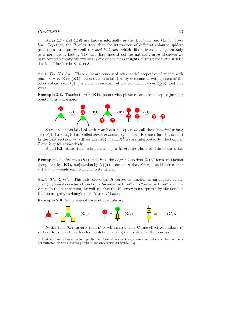
2.2.4. The K-rules. These rules are concerned with special properties of spiders withphase α = π. Rule (K1) states that dots labelled by π commute with spiders of theother colour, i.e., X1

1 (π) is a homomorphism of the comultiplication Z12 (0), and vice

versa.

Example 2.6. Thanks to rule (K1), points with phase π can also be copied just likepoints with phase zero:

π(S1)=

π (K1)=

ππ(B1)= π π

(S1)= π π

Since the points labelled with π or 0 can be copied we call these classical points;then Z1

1 (π) and X11 (π) are called classical maps.§ (Of course, K stands for “k lassical”.)

In the next section, we will see that Z11 (π) and X1

1 (π) are interpreted by the familiarZ and X gates respectively.

Rule (K2) states that dots labelled by π invert the phase of dots of the othercolour.

Example 2.7. By rules (S1) and (S2), the degree 2 spiders Z11 (α) form an abelian

group, and by (K2), conjugation by X11 (π)— note here that X1

1 (π) is self-inverse sinceπ + π = 0 —sends each element to its inverse.

2.2.5. The C-rule. This rule allows the H vertex to function as an explicit colourchanging operation which transforms “green structures” into “red structures” and viceversa. In the next section, we will see that the H vertex is interpreted by the familiarHadamard gate, exchanging the X and Z bases.

Example 2.8. Some special cases of this rule are:

=

H

H

H

(C1) ブ =

ブH

(C2)H

H

(C3).

Notice that (C3) asserts that H is self-inverse. The C-rule effectively allows Hvertices to commute with coloured dots, changing their colour in the process.

§ That is, classical relative to a particular observable structure; these classical maps then act as apermutation on the classical points of the observable structure [25].

CONTENTS 14

2.2.6. The D-rules. The (D2) rule states that two black diamonds are equal to a loopof wire, itself the result of composing a cup and a cap. We will see in the next sectionthat the loop represents the dimension of the underlying Hilbert space, and spacialjuxtaposition is a form of multiplication, justifying the name

√D for the diamond.

The (D1) rule ‘almost follows’ from the other rules:

(S1)=

(B1)=

which would yield the desired result if could be cancelled.

2.3. Interpreting the zx-calculus in Hilbert space

Given a diagram D with n inputs and m outputs, we construct a corresponding linearmap D : Qn → Qm as follows.

Definition 2.9 (Interpretation of generators). If D consists of just a singlegenerator—that is, one of 1Q, σQ, ηQ, εQ, Znm(α), Xn

m(α), H, or√D—then its

corresponding linear map is as shown below:

=

(1 00 1

)=

1 0 0 00 0 1 00 1 0 00 0 0 1

= |00〉+ |11〉 = 〈00|+ 〈11|

n︷ ︸︸ ︷ブ︸ ︷︷ ︸m

::

n︷ ︸︸ ︷

|0 . . . 0〉 7→m︷ ︸︸ ︷

|0 . . . 0〉|1 . . . 1〉 7→ eiα |1 . . . 1〉others 7→ 0

n︷ ︸︸ ︷ブ︸ ︷︷ ︸m

::

n︷ ︸︸ ︷

|+ . . .+〉 7→m︷ ︸︸ ︷

|+ . . .+〉|− . . .−〉 7→ eiα |− . . .−〉others 7→ 0

H = 1√2

(1 11 −1

)=√

2

Example 2.10. The generators Z11 (π) and X1

1 (π) are the Pauli Z and X matrices:

π =

(1 00 −1

)π =

(0 11 0

),

Example 2.11. The generators Z12 and X1

2 are interpreted as follows:

::

{|0〉 7→ |00〉|1〉 7→ |11〉 and ::

{|+〉 7→ |+ +〉|−〉 7→ | − −〉

CONTENTS 15

giving the maps which copy the Z-basis vectors and the X-basis vectors respectively.Consider Z0

1 . Notice that its corresponding linear map sends 1 7→ |0〉 and also1 7→ |1〉, hence by linearity we obtain 1 7→ |0〉+ |1〉 =

√2 |+〉. The complete set of Z-

and X-basis vectors is show below.

=√

2 |+〉 , π =√

2 |−〉 , =√

2 |0〉 , π =√

2 |1〉 .

Definition 2.12 (Interpretation of compound diagrams). If D consists of severalgenerators there are two cases:

• if D = D1 ⊗D2 then D = D1 ⊗D2;

• if D = D1 ◦D2, then D = D1 ◦D2.

The order in which we divide the diagram into pieces does not matter to thefinal result, so long as the “cuts” do not pass through any vertices, nor any pointswhere wires cross, nor any points of inflection of a wire—more accurately: just thoseinflection points were the gradient of the wire changes sign. (These last two may bethought of as the “vertices” defining σQ, and ηQ and εQ respectively.)

Example 2.13. The following diagram can be divided up as follows:

ブ プπ=

ブ プπ=

ブ π⊗

⊗

プ

=

(◦(ブ ⊗ π

))⊗

(◦

)⊗プ

giving the linear map

D =

1 0 0 00 0 1 00 1 0 00 0 0 1

(e−iα2

(cos α2 i sin α

2i sin α

2 cos α2

)⊗(

1 00 −1

))

⊗ 1√2

1 00 00 00 1

( 1 0 0 10 1 1 0

)⊗ e−iβ2

(i sin β

2

cos β2

).

Unlike the diagram, the resulting matrix is rather large (16 × 32) so it is not shownhere. Any other factorisation of the diagram, for example,

ブ プπ=

(⊗ ⊗ プ

)◦(ブ ⊗ π ⊗ ⊗

)

produces the same interpretation.

Example 2.14. According to the T-rule, the diagram of Example 2.13 above isequivalent to the one shown below:

CONTENTS 16

ブ プπ

As one might hope, this gives the same interpretation.

Remark 2.15. A linear map f : C→ C is completely determined by the value f(1).For this reason, and since Q0 = C, the Hilbert space interpretation of a diagram withno inputs or outputs—a map from C to itself— is simply a complex number.

Proposition 2.16 (Soundness). If diagrams D1 and D2 are equal according to theequational rules of the zx-calculus then D1 = D2.

This proposition can largely be verified by computing the maps corresponding toleft and right sides of each of the equational rules given in Figure 1, and observingthat they are equal. However, to show that the T-rule is correct, different techniquesare required. We will return to this point, and the (non)-issue of the factorisationorder, in Section 4.3.

The converse of Proposition 2.16 is false: there exist diagrams D1 and D2 whichrepresent the same linear map but which are not equal by the rules of the zx-calculus.For example, the following diagrams are not equivalent in the calculus:

H 6=-π/2π/2π/2

,

but their interpretation as linear maps is the Euler-angle decomposition,

H = Z11 (π

2) ◦X1

1 (π

2) ◦ Z1

1 (−π2

) .

This equation is equivalent to Van den Nest’s theorem on local complementation ofgraph states [75], as shown elsewhere by Perdrix and one of the authors [36].

We remark upon this fact for two reasons. Firstly, as warning that not every truefact about Hilbert space quantum mechanics can be derived using the zx-calculus,although a great many equations used in quantum information processing can be.Secondly, since the equational theory of the zx-calculus is strictly weaker than thatof Hilbert spaces, it is more general. Therefore there are models of the calculus whichare distinct from the usual Hilbert space interpretation of quantum mechanics. Allsuch models contain a large fragment of quantum mechanics—viewed as an equationaltheory—but facts like Van den Nest’s theorem need not hold.

Remark 2.17. The points in the calculus are not normalized. This is required forreasons of simplicity; if we were to normalize σQ and ηQ, then the (T1) rule wouldrequire additional scalar multipliers, and hence so would the (S1) rule, and so on.

2.4. Universality of the zx-calculus

We claim that we now have enough expressive power to write down any arbitrarylinear map from n qubits to m qubits. The green and red phases, respectively:

ブ = Z11 (α) =

(1 00 eiα

)(2)

ブ = X11 (α) = e−iα/2

(cos α2 i sin α

2i sin α

2 cos α2

)(3)

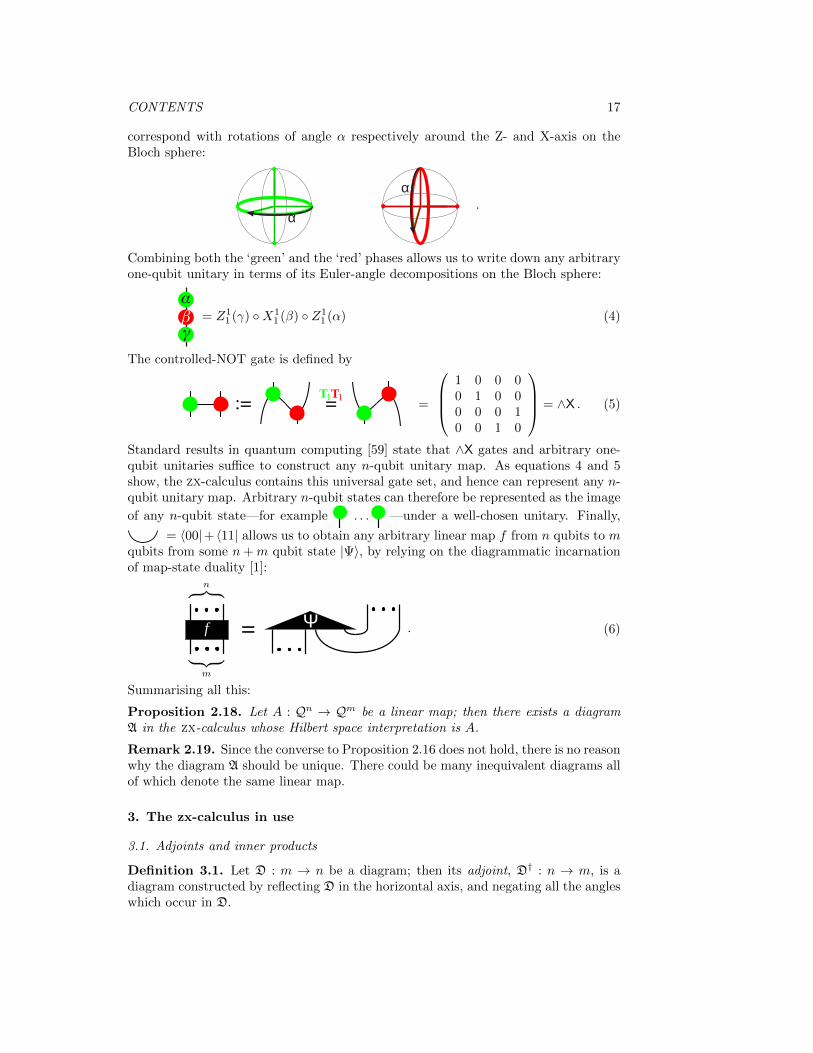
CONTENTS 17

correspond with rotations of angle α respectively around the Z- and X-axis on theBloch sphere:

α

α.

Combining both the ‘green’ and the ‘red’ phases allows us to write down any arbitraryone-qubit unitary in terms of its Euler-angle decompositions on the Bloch sphere:

ブプベ

= Z11 (γ) ◦X1

1 (β) ◦ Z11 (α) (4)

The controlled-NOT gate is defined by

1T 1T=

1 0 0 00 1 0 00 0 0 10 0 1 0

= ∧X . (5)

Standard results in quantum computing [59] state that ∧X gates and arbitrary one-qubit unitaries suffice to construct any n-qubit unitary map. As equations 4 and 5show, the zx-calculus contains this universal gate set, and hence can represent any n-qubit unitary map. Arbitrary n-qubit states can therefore be represented as the image

of any n-qubit state—for example . . . —under a well-chosen unitary. Finally,

= 〈00|+ 〈11| allows us to obtain any arbitrary linear map f from n qubits to mqubits from some n+m qubit state |Ψ〉, by relying on the diagrammatic incarnationof map-state duality [1]:

n︷ ︸︸ ︷Ψf .

︸ ︷︷ ︸m

(6)

Summarising all this:

Proposition 2.18. Let A : Qn → Qm be a linear map; then there exists a diagramA in the zx-calculus whose Hilbert space interpretation is A.

Remark 2.19. Since the converse to Proposition 2.16 does not hold, there is no reasonwhy the diagram A should be unique. There could be many inequivalent diagrams allof which denote the same linear map.

3. The zx-calculus in use

3.1. Adjoints and inner products

Definition 3.1. Let D : m → n be a diagram; then its adjoint, D† : n → m, is adiagram constructed by reflecting D in the horizontal axis, and negating all the angleswhich occur in D.

CONTENTS 18

A diagram D is called self-adjoint if D = D†, and unitary if D ◦D† = 1⊗nQ and

D† ◦D = 1⊗mQ .

Example 3.2. Given the diagram D, we form its adjoint D† as shown:

D =ブ プ

D† =-ブ -プ

We claim that D is unitary. Half of the required proof is shown below.

ブ プ-ブ -プ

(S1)=

(S2)=

(S1)=

(B′)=

(S2)=

The ‘horizontal application’ of the B′-rule can be decomposed as follows:

(T)=

(S1)=

(B′)=

(S1)=

(T)=

from which it follows that pairs of wires between green and red dots can be eliminated.It remains to show that D ◦D† = 1Q2 .

The following is self-evident:

Proposition 3.3. Let D be some diagram. Then (i) D†† = D; (ii) if D = A ◦ B,then D† = B† ◦ A†; and (iii) if D = A⊗B, then D† = A† ⊗B†.

Proposition 3.4. If D : m → n denotes the linear map D : Qm → Qn, then theadjoint diagram D† denotes D†, the usual linear algebraic adjoint of D.

Corollary 3.5. If a diagram is self-adjoint or unitary so is its corresponding linearmap.

Recall that any diagram D : 0 → n has a (possibly unnormalised) n-qubit stateas its Hilbert space interpretation; such diagrams therefore correspond to kets |D〉 inDirac notation. Since Dirac’s bra is the adjoint of a ket, we now see how to define theinner product of two diagrams. Given A,B : 0→ n we have

〈A | B〉 = A† ◦B .

The resulting diagram (A† ◦B) has no inputs or outputs, hence by Remark 2.15, itdenotes a complex a number, as required.

Example 3.6. We can compute the inner product of Z01 (α) with itself.

ブ

-ブ(S1)=

(S1)=

(S2)=

(D2)=

The result is 2 because the “states” are not normalised.

CONTENTS 19

Example 3.7. Let j, k ∈ {0, π}. We compute the inner product of Z01 (k) and X0

1 (j).

j

k(S1)=

kj

(K2)=

k

j (K1)= k

(K1)=

(D1)=

Since the result is independent of j and k, this calculation shows that the X and Zbases are mutually unbiased.

Example 3.8. Suppose that U is a diagram encoding some complicated unitaryoperation U , acting on n + 1 qubits. Suppose its input is |00 · · · 0〉: what is theamplitude for observing the output |1〉 at its last output? We need to compute:

〈00 · · · 0|U†(1Qn ⊗X)U |00 · · ·〉 = π

. . .

. . .

. . .

When U is presented using the generators of the zx-calculus, great simplification is(usually) possible, making this expression (usually) easy to compute.

3.2. Quantum Circuits

As we have already seen in Section 2.4, the zx-calculus can represent the basic gatesused in quantum circuits. The rules of the calculus can give short graphical proofs ofmany circuit identities.

3.2.1. The ∧X gate. We have already seen the controlled-NOT gate:

∧X = .

It is manifestly self-adjoint. We can prove that it is also unitary:

∧X ◦ ∧X =(S1)=

(B′)=

(S2)= = 1⊗2Q ,

An elementary exercise is to show that a sequence of three ∧X gates can be usedto swap to qubits. A graphical proof of this fact is given below.

(T)=

(B2)=

(S1)=

(B′)=

(S2)=

CONTENTS 20

While this is a well-known property for ∧X, our proof holds in much greater generalitythan qubits, since as we will see in the remainder of this paper, the graphical calculusapplies in much greater generality. This example relies on the bialgebra law (B2),which is a stronger principle than the Hopf law (B’) used in the previous example.The relationship between these two laws will be spelled out in Section 9.

In Section 2.4 the ∧X gate was introduced by checking that its diagram denotedthe correct linear map. However we can describe ∧X by the following “behaviouralspecification”: when the control input is |0〉, the target qubit is left unchanged; when

the control qubit is |1〉, the target qubit is flipped. Letting k represent one of the two

red classical points, that is, either = |0〉 or π = |1〉, we can supply a qubit to the

control input (the left input, connected to the green dot), and obtain the followingproof:

k(K1)+(B1)

=k

k (S1)=

k

k=

iff k =

π π iff k = π

Notice that in each case the control qubit passes through the gate unchanged, whilethe target input is either the identity, or the Pauli X, depending on the value of thecontrol qubit, thus meeting the specification. Further, the colour symmetry of this

proof demonstrates that, if we operate in the Z-basis (i.e., |+〉 = and |−〉 = π )

the role of left and right are exchanged.

3.2.2. The ∧Z gate. Since Z = HXH we can obtain the ∧Z gate from the ∧X gateby conjugating the target qubit with H gates, as shown below:

∧Z =

1 0 0 00 1 0 00 0 1 00 0 0 −1

=

H

H

= H .

We can immediately read off two properties of this gate from its graphicalrepresentation: it is self-adjoint, and it is symmetric in its inputs. It is also unitary:

H

H (S1)=

H

H (C)=

H

H(B′)=

H

H(S2)=

H

H(C)=

3.2.3. The quantum Fourier transform. Lying at the centre of many quantumalgorithms—including Shor’s famous factoring algorithm [71]—the quantum Fouriertransform is one of the most important quantum processes. The equations of thediagrammatic calculus are strong enough to simulate it.

To write down the required circuit, we must realise a controlled phase gate, wherethe phase is an arbitrary angle α; this is shown below—the control qubit is on the

CONTENTS 21

left. (One can prove the correctness of this diagram using a behavioural descriptionin a similar fashion to the treatment of the ∧X in Section 3.2.1.)

∧Zα =

1 0 0 00 1 0 00 0 1 00 0 0 eiα

= -ブ/2

ブ/2

The only gates which are required to construct the circuit implementing the quantumFourier transform are the Hadamard and the ∧Zα—see for example [59]. The circuitfor the 2-qubit QFT is shown below.

QFT2 = -π/4

π/4

H

H

How can we simulate this circuit? First, we choose an input state, in this case

|10〉 = π ; then we simply concatenate the input to the circuit, and begin

rewriting according to the equations of the theory, as shown below.

QFT2 ◦ |10〉 = -π/4

π/4

H

H

π

(K)= -π/4

π/4

H

H

π

ππ

(S1)= -π/4

π/4

H

H

π

π

π(K2)=

π/4

π/4

H

H

π ππ

(S)= π/4

π/4

H

H

π(C)= π/4

π/4π

(S1)= π/2

π

The final diagram in the sequence is simply the tensor product (|0〉−|1〉)⊗(|0〉+i |1〉),which is indeed the desired result. In passing we remark upon another feature of thegraphical language: since the last diagram is a disconnected graph, it represents aseparable quantum state.

3.3. Measurement-based quantum computing

Measurement-based quantum computation [49] uses the state-changing effect ofquantum measurements to carry out the computation, typically propagating thesechanges through entangled states. The simplest example is the teleportation protocol[8] which can be viewed as the identity function computed via a Bell state. A morepowerful model is Raussendorf and Briegel’s one-way quantum computer [64, 65],which provides a computationally universal model almost entirely based on single-qubit measurements acting on a large cluster state.

CONTENTS 22

The graphical notation of the zx-calculus is ideal for representing these entangledstates, and its equations accurately capture the changes in these states induced bymeasuring their constituent parts.

Remark 3.9. The zx-calculus as presented in this section, cannot represent thenon-deterministic behaviour of measurements. Rather, we replace measurements byprojections onto some particular outcome. One could view this as post-selection, butit would more accurate to understand that each diagram represents a one particularrun of an experiment, and the particular outcome that was measured, rather thanaveraging over all possible runs. The restriction to pure states is not an instrinsiclimitation of this approach. It is a deliberate choice, made in order to simplifythe presentation of the calculus. The formal apparatus used here was introduced in[27] to represent classical control structure and the branching behaviour of quantummeasurements. In Section 12 we present three extensions to the calculus to handlenon-determinism and mixedness.

3.3.1. The teleportation protocol. The teleportation protocol [8] consists of two maincomponents: the preparation of the Bell state, and the Bell basis measurement. Asdescribed in Section 2.3, the (unnormalised) Bell state is represented by a cap, andits corresponding projection by a cup:

|00〉+ |11〉 = , 〈00|+ 〈11| = .

Combining these two elements, we obtain an almost trivial proof of the correctness ofteleportation, in the case where Alice observes |00〉+ |11〉.

in

outAlice

Bob

=

in

outAlice

Bob

The role of classical communication is hidden in this picture, but it is revealed by amore detailed look at the Bell basis measurement. Let α, β ∈ {0, π}. Ranging overthe 4 possible (α, β) pairs in the diagram below gives the 4 possible outcomes of a Bellbasis measurement:

{ 〈Ψ+| , 〈Ψ−| , 〈Φ+| , 〈Φ−| } =

H

ブ プ| α, β ∈ {0, π}

(Notice that the boxed part of the diagram is simply the circuit which rotates the Bellbasis onto the X-basis.) This description of the protocol displays the Pauli errors thatare introduced if Alice observes the other possible outcomes.

in

out

Bob

H

Ơ ơ

Alice

=

in

out

Bob

ブ

Alice

プ=

in

out

Bobブ Alice

プ

CONTENTS 23

From this we can derive a complete description of the protocol, and show, includingBob’s corrections, which are classically correlated to Alice’s observations.

in

out

Bob

H

Ơ ơ

Alice

ơƠ

=

in

out

BobAlice

プブ

ブプ

=

in

out

BobAlice

ブ

ブ=

in

out

BobAlice

The first equation is the preceding derivation collapsed into one step, while the lasttwo equations use the spider rules and the fact that 2α = 2β = 0.

3.3.2. The state transfer protocol. This protocol was introduced by Pedrix [62] toreduce the resources required for measurement based quantum computing. The coreof the protocol is a measurement which projects onto a 2-dimensional eigenspace:

S=

1 0 0 00 0 0 00 0 0 00 0 0 1

= PZ⊗Z (7)

It is easily seen that PZ⊗Z is self-adjoint and idempotent:

PZ⊗Z ◦ PZ⊗Z =S S

= PZ⊗Z , (8)

and hence a projector.Consider now a protocol, which initially assume two qubits, one in an unknown

state = |ψ〉 and one in the state = |+〉. We want to transfer |ψ〉 from the first

qubit to the second, and this can be done by means of two projections:

measurement bra

measurement projector

ancillary qubit statequbit in unknown state

since by application of the S-rule we have:

.

The protocol can be extended by performing the second, single-qubit measurement inthe phase-shifted basis |0〉 ± eiα |1〉.

measurement bra with phase ブブ(S)

=

(1 00 eiα

)

CONTENTS 24

This minor change allows the protocol to apply an arbitrary Z-rotation to its input;the protocol can be modified in the obvious way to perform an X-rotation, and henceany single-qubit unitary.

3.3.3. Multipartite states. In our graphical language, a quantum state is nothingmore than a diagram with no inputs; the outputs correspond to the individual qubitsmaking up the state. The interior of the diagram—i.e. its graph structure—describeshow these qubits are related. This notation is ideal for representing large entangledstates.

Cluster states, which are used in measurement-based quantum computing [65],can be prepared in several ways and the zx-calculus provides short proofs of theirequivalence. For example, the original scheme describes a ∧Z interaction betweenqubits initially prepared in the state |+〉; in our notation this is Z0

1 , or . Hence aone-dimensional cluster state can be presented diagrammatically as:

H

H

H

H

H

H. . . .

. . . .

where the boxes delineate the individual |+〉 preparations and ∧Z operations.Alternatively, the cluster state can be prepared by applying a Hadamard gate to onepart of a Bell pair to obtain states of the form |Φ〉 = |0+〉+ |1−〉, and then “fusing”these entangled pairs [76]. The required fusion operation is exactly

: Q⊗Q → Q ::

|00〉 7→ |0〉|11〉 7→ |1〉

|01〉, |10〉 7→ 0, (9)

and a 1D cluster prepared with this method looks like:

H H H H

. . . .. . . .

.

Again, dashed lines indicate the individual components. While conventional methodsrequire some calculation to show that these methods of preparation produce thesame state, using the spider theorem, the two diagrammatic forms are immediatelyequivalent:

H H H HH

H

H

H

H HH H= = .

From the example of the 1D cluster, it’s easy to see how to construct diagramscorresponding to arbitrary graph states. Indeed given a graph state |G〉, withunderlying graph G, we represent |G〉 by the same graph G, with green dots at eachvertex, and H gates on each edge; to complete the construction we must add oneoutput wire at each green vertex.

While graph states are important in measurement-based quantum computation,they are not the only kind of interesting entangled states. As an illustration ofuniversality of the graphical language, we present graphical representatives of the two

CONTENTS 25

non-comparable classes of genuine three qubit entangled states‖. As can be directlyread from the interpretation given in Section 2.3, the GHZ state is simply a three-legged spider:

|GHZ〉 = |000〉+ |111〉 = .

The simple form of this state hints at its importance in the algebraic structures tobe introduced later in this paper. This algebraic role, particularly in relation to thephase group, has been used to explain non-locality [20]. The W state, however, is lessobvious:

|W〉 = |001〉+ |010〉+ |100〉 = π/3π/3π/3 .

This representation supports the intuition that while the GHZ state is a globallyentangled, the W is rather to be conceived as a pairwise entanglement between eachpair of qubits that make up the three-partite system [38]. The algebraic properties ofthe W state have been studied elsewhere by Kissinger and one of the authors [21].

3.3.4. The one-way model The graphical language is ideal for studying differentmodels of quantum computation in the same setting. In this section we will presentseveral computations using the one-way model [64], and translate them into equivalentquantum circuits using the rules of zx-calculus. We use the measurement calculusnotation introduced by Danos, Kashefi, and Panangaden [30], and borrow theirexamples.

For our purposes, a measurement calculus program, called a pattern, consists ofa sequence of commands of the following kinds:

• Ni – initialise qubit i to the state |+〉.• Eij – apply a ∧Z operation to qubits i and j.

• Mαi – measure the qubit i in the basis |0〉 ± eiα |1〉.

The commands occur in the order given: first initialisations, then entanglement, thenmeasurement. Any quibit which is not initialised is an input; any not measured is anoutput.

Since, in the zx-calculus, measurements are replaced by projections, theconditional operations of the measurement calculus have been omitted; see Section 12and [37] for a more complete treatment. We make the convention that the observedoutcome of each measurement will be the +1 outcome—that is, the projection onto|0〉 + eiα |1〉. With this convention the elements of the measurement calculus can betranslated by the following table:

Ni Eij Mαi

H -ブ‖ The GHZ state cannot be converted to the W state by means of stochastic local operations andclassical communication, nor vice versa. States which can be so-interconverted are called SLOCC-equivalent : up to SLOCC-equivalence the GHZ and W are the only 3-qubit states with 3-partyentanglement [38].

CONTENTS 26

Example 3.10. Consider a measurement-based program involving 4 qubits, whichcomputes a ∧X gate upon its inputs. In the syntax of the measurement calculus thispattern is written:

M02M

04E13E23E34N3N4.

Reading from right to left, this specifies that qubits 3 and 4 should be prepared in a|+〉 state, then ∧Z operations should be applied pairwise between qubits 1 and 3, 2and 3, and 3 and 4; finally X basis measurements should be performed upon qubits 2and 4. Qubits 1 and 2 are the inputs and qubits 1 and 4 are the outputs. We representthis pattern diagrammatically as:

H

H

H

Inputs 1 and 2

Output 1 Output 4

gates

The spider theorem allows this one-way program to be rewritten to a ∧X gate in threesteps:

H

H

H

H

H=

H

= = .

Example 3.11. Our next example is a one-way program implementing an arbitrary 1-qubit unitary. Recall that any single qubit unitary map U has an Euler decompositionas such that U = ZγXβZα. Such a unitary can be implemented by the following 5-qubit measurement pattern:

Mγ3M

β2M

α1 E12E23E34E45N2N3N4N5 .

The graphical form of this pattern is shown below:

HH

HH

α β γ

Input 1

Output 5

gates

.

A sequence of simple rewrites shows that the one-way program intended to computesuch a unitary does indeed produce the desired map.

HH

HH

ブ プ ベ

(S1)= HH HHブ プ ベ (C)

= ブ ベプ

CONTENTS 27

Remark 3.12. The reader may object that the “post-selection” of one particular setof measurement outcomes reduces the number of diagrams significantly, and thus givesa misleading air of feasibility to these techniques. In practice the pure state version ofthe zx-calculus needs only minor extension to handle the full behaviour of the one-waymodel, without any combinatorial explosion. We sketch this extension in Section 12;the full details can be found in [37].

4. Symmetric monoidal categories and graphical reasoning

The preceding sections presented the zx-calculus as a fait accompli, without anyserious justification for its axioms, other than its utility in certain calculations. Thissection, and those that follow, will put down the firm mathematical foundation uponwhich the calculus is built. This section will outline the basic concepts of symmetricmonoidal categories (smcs) without going into too much technical detail; we aim toprovide the reader with just enough background to follow the subsequent material,and provide many references where complete and detailed expositions can be found.

A category consists of objects A,B,C, . . . and, for each pair of objects A,B, acollection of morphisms f, g, h, . . . : A→ B. From a physical perspective, the objectscan be thought of as physical systems and each morphism f : A → B as a physicalprocess which transforms a system of type A to a system of type B. Here, ‘type’should not be confused with ‘state’. E.g. type could be qubit, or field, or a certainclassical system, and each of these admits many states. For a computer scientist, theobjects may be data-types, and f : A → B would be a program accepting input oftype A and producing output of type B. In mathematics the objects are typicallystructures of a certain kind, e.g. sets, or groups, or vector spaces, and f : A→ B is astructure preserving map, e.g. a function, or a group homomorphism, or a linear map.

Pairs of morphisms where the domain of one matches the codomain of the othermay be composed : for each such pair, f : A → B and g : B → C, we write thecomposite g ◦ f : A → C. In the case of physical processes g ◦ f can be interpretedas ‘process g after process f ’; in the case of structure preserving maps compositionof morphisms is just ordinary function composition. Composition is assumed tobe associative. One also assumes the existence of units for this composition; moreprecisely, for all A there exist identity morphisms 1A : A → A such that for allf : A→ B and all g : B → A we have f ◦1A = f and 1A ◦g = g. As a physical processthis would stand for the void process, or in operational terms, “doing nothing”.¶

In addition to the ‘sequential’ composition operation − ◦ −, an smc also comeswith ‘parallel’ composition − ⊗ −. For two physical systems A and B there is acompound system A ⊗ B and for each pair of physical processes f : A → C andg : B → D there is a compound process f ⊗ g : A ⊗ B → C ⊗D. For mathematicalobjects ⊗ then indicates a compound mathematical object of a certain kind, builtfrom two ‘smaller’ ones, e.g. using the Cartesian product of sets, or the direct productof groups, or the tensor product of vector spaces. One also assumes a unit object Isuch that composing A with I leaves A essentially unchanged. Finally, for each pair ofobjects A and B one assumes a swap morphism σA,B : A⊗B → B⊗A. The remainingaxioms of an smc then play two roles:

• bifunctoriality states how the two modes of composition interact;

¶ Obviously, “doing nothing” in the lab is a very difficult (if not impossible) task, e.g. preventingdecoherence is the biggest stumbling block to building a quantum computer.

CONTENTS 28

• the existence of a number of natural isomorphisms and coherence conditionsbetween these formalise the meaning of ‘essentially’ when saying that A ⊗ I is‘essentially’ the same as A.+ The swap morphisms are also natural isomorphisms;these embody the canonical connection between A⊗B and B ⊗A.∗

All of these conditions have a straightforward physical interpretation and are satisfiedfor most standard mathematical constructions of compound objects.

Since there are two modes of composition, smcs naturally lend themselves to a 2-dimensional syntax we call the graphical (or diagrammatic) calculus, where the verticalaxis corresonds the sequential composition “◦”, and the horizontal axis to the tensorproduct “⊗”. Moreover, when expressed in the graphical language, the coherenceconditions for smcs become trivial as a consequence of some very powerful theorems,so play no further role in this paper. Hence, while below we do state the symbolicdefinition of a symmetric monoidal category, it is not crucial for the remainder of thispaper. The graphical language is both clearer and closer to the physical intuition; thereader who prefers the graphical langauge can skip ahead to Section 4.3.

A more detailed presentation of the physical intuition behind smcs can be found in[14, 24, 17]; [24] is an extensive tutorial specifically written to provide the appropriatebackground on the kind of category that is required for this paper. Other tutorialsthat may be of help are [3, 6]. Mac Lane’s standard textbook on category theoryappeals to a mathematical audience [57].

The graphical calculus for smcs can be traced back to Penrose’s work in theearly 1970’s [61], but was turned into a formal discipline only after the work of andFreyd and Yetter, and Joyal and Street, around 1990 [42, 47]. A physicist friendlypresentation is again in [14, 24, 17], and a specifically targeted tutorial is again [24]. Arecent comprehensive survey paper on graphical languages for more general monoidalcategories, which settles a number of caveats of earlier literature, is [69]. The readerinterested in learning more may also find [6, 53, 73] helpful.

4.1. Symmetric monoidal categories

Definition 4.1. A category C consists of a class of objects denoted |C|, and for eachpair of objects A,B ∈ |C|, a set C(A,B) of morphisms or arrows. For each tripleA,B,C ∈ |C| there is composition

− ◦ − : C(A,B)×C(B,C)→ C(A,C),

which is associative, i.e. (f ◦ g) ◦ h = f ◦ (g ◦ h), and for each object A ∈ |C| thereis an identity morphism 1A : A → A, that is, i.e. for all f ∈ C(A,B) we havef ◦ 1A = f = 1B ◦ f .

A morphism f : A→ B has domain A and codomain B. We will sometimes referto objects as types, to A as the input type, and to B as the output type.

In order to precisely state the definition of an smc we need to introduce twoauxilliary concepts: functors and natural transformations. While these definitions

+ For example, while for all practical purposes the sets X× (Y ×Z) and (X×Y )×Z are equivalent,they are strictly speaking not the same: the first one contains elements of the form (x, (y, z)) while thesecond one contains elements of the form ((x, y), z). Making this notion of equivalence mathematicallyprecise is what makes the explicit definition of an smc somewhat heavy-handed.∗ Now, (x, y) and (y, x) are not anymore ‘essentially the same’, but they still are canonically connectedvia the operation ‘swapping elements’.

CONTENTS 29

may seem rather abstract, the only examples of them that will be needed are familiarones: the tensor product, and isomorphisms between tensor products of objects.

By explicitly stating some basic category-theoretic notions the reader may get asense of why even many mathematicians consider category theory as ‘very abstract’;in contrast, the diagrammatic calculus shows that specific parts of category theory,namely smcs and in particular their graphical calculus, can make certain mathematicalstructures way more intuitive and easier to manipulate.

Definition 4.2. Let C and D be categories. A functor F : C→ D is defined by (i)for each object A in |C| an object F (A) in |D|, and (ii) for every arrow f : A→ B inC an arrow F (f) : F (A)→ F (B) in D such that:

F (f ◦ g) = F (f) ◦ F (g) and F (1A) = 1F (A) .

Remark 4.3. A variation on the idea of functor is a contravariant functor, whichreverses the direction of arrows; that is, F assigns to every arrow f : A→ B in C anarrow F (f) : F (B)→ F (A) in D.

Definition 4.4. A bifunctor is a functor of two arguments F : C×C′ → D, that isa functor in each argument separately, i.e., for all objects X and arrows f : A → B,g : B → C in C, and all objects X ′ and arrows f ′ : A′ → B′, g′ : B′ → C ′ in C′, wehave:

F (g, 1X′) ◦ F (f, 1X′) = F (g ◦ f, 1X′) ,F (1X , g

′) ◦ F (1X , f′) = F (1X , g

′ ◦ f ′) ,which additionally satisfies

F (g, 1B′) ◦ F (1B , f′) = F (1C , f

′) ◦ F (g, 1A′) ,

F (1A, 1B′) = 1F (A,B′).

In essence, a functor is a map between categories that preserves the structure ofthe category, i.e. composition and identities. We will also need maps between functors.

Definition 4.5. Let F,G : C→ D be functors; a natural transformation τ : F ⇒ Gis a family of arrows in D, τA : F (A)→ G(A), indexed by the objects of C, such thatthe following square commutes:

F (A)τA- G(A)

G(A)

F (f)

?

τB- G(B) ,

G(f)

?

for all arrows f : A → B in C. A natural isomorphism is a natural transformationwhere each of the τA is an isomorphism; that is, there exists a morphism τ−1A suchthat τA ◦ τ−1A and τ−1A ◦ τA are both identities.

Notation and terminology: Each directed path in the diagram above determines acomposition of two maps: G(f) ◦ τA on the upper path, and τB ◦ F (f) on the lower.The phrase “the square commutes” means that both paths in this directed graph areequal, i.e. G(f) ◦ τA = τB ◦ F (f).

If two objects in category are naturally isomorphic then they are isomorphic ‘forstructural reasons’ and not because of any particular details of the objects themselves.The follow definition provides a key example.

CONTENTS 30

Definition 4.6. A monoidal category (C,⊗, I) is a category C equipped with abifunctor −⊗− : C×C→ C, a distinguished unit object I, natural unit isomorphisms

λA : A ' I⊗A and ρA : A ' A⊗ I ,

and a natural associativity isomorphism

αA,B,C : A⊗ (B ⊗ C) ' (A⊗B)⊗ C ,which are subject to certain coherence equations, which we omit.

The bifunctor −⊗− is called the tensor product or monoidal tensor. The mapsλ, ρ, α are called the monoidal structure maps. A monoidal category is called strictwhen the structure maps are all identities; that is, when the objects made isomorphicby λ, ρ, α are in fact equal. The following theorem by Mac Lane justifies our omissionof the coherence equations for the structure maps.

Theorem 4.7. Every monoidal category is equivalent to a strict monoidal category.

For details we refer the reader to [57]. Hence forward all the monoidal categorieswe consider will be strict, although we will frequently use the symbols λA and ρAfor clarity, for example, when composing an arrow of type B → A with one of typeA⊗ I → C.

Definition 4.8. A symmetric monoidal category is a monoidal category equippedwith a natural symmetry isomorphism

σA,B : A⊗B ' B ⊗Asuch that σ−1A,B = σB,A, and again subject to some coherence conditions which weomit.

If C is an smc then σ is counted among its structure maps. Unlike the otherstructure maps σ cannot be replaced by the identity without losing essential structure.We again refer the reader to [57] for the details of the coherence conditions; they aresummarised in the following theorem [52]:

Theorem 4.9 (Kelly-Mac Lane). Let f and g be parallel natural isomorphisms in asymmetric monoidal category, both constructed from identities and the structure mapsby tensoring and composition; then f = g.

Essentially this result says that when one uses the structure maps to permute thefactors of a tensor product, only the permutation matters, not how it was constructed.]

The preceding definitions may seen rather intimidating to those unfamiliar withcategory theory, but there is no need to be alarmed: smcs are among the mostubiquitous of mathematical structures!

Example 4.10. The smc (FdHilb,⊗,C), often written simply as FdHilb, hasfinite dimensional Hilbert spaces as objects and linear maps as its morphisms, whichcompose by ordinary composition of linear maps. The familiar Kronecker tensorproduct is the monoidal tensor, and the the field of complex numbers C —whichis a one-dimensional Hilbert space over itself— is the tensor unit.

] The restriction to natural isomorphisms prevents different permutations from being identified.For example, 1A⊗A and σA,A cannot be identified, despite being parallel arrows, since they arecomponents of different natural transformations, namely 1⊗1 : A⊗B ⇒ A⊗B and σ : A⊗B ⇒ B⊗A;again, see [57] for details.

CONTENTS 31

The requirement that the monoidal tensor be a bifunctor reduces to the followingwell-known property of linear maps:

(f ⊗ g) ◦ (h⊗ k) = (f ◦ h)⊗ (g ◦ k).

We indeed also have H ' C⊗H via the natural isomorphism:

λH : H → C⊗H :: |ψ〉 7→ 1⊗ |ψ〉 ,λ−1H : C⊗H → H :: c⊗ |ψ〉 7→ c|ψ〉 ,

where naturality means that for all f : H → H′ the following diagram commutes:

H λH- C⊗H

H′

f

?λ′H- C⊗H′

1C⊗f

?

i.e. (1C⊗f)◦λH = λH′◦f . In FdHilb, it is easily checked that natural transformationsare always basis-independent. The reader may consult [24] for a detailed descriptionof (FdHilb,⊗,C).

Example 4.11. Let (ZX,⊗, 0) denote the smc whose objects are natural numbers,and whose arrows f : n→ m are diagrams of the zx-calculus, as described in Section 2,with n inputs and m outputs. The identity arrows are diagrams consisting of straightwires from inputs to outputs, and composition is achieved by plugging inputs tooutputs.

The tensor product on objects is addition n ⊗m := n + m, and the unit objectis zero: n⊗ 0 = n+ 0 = n. Tensor product of two diagrams is juxtaposition, and theidentity map 10 is just the empty diagram. By its construction, ZX is evidently astrict monoidal category. We leave to the reader the task of constructing the symmetrymaps σn,m from crossings of wires.

We remark in passing that the assignment from a diagram D to its correspondinglinear map D, described in 2.3, defines a functor from ZX to FdHilb.

In the categorical setting the internal structure of the objects is hidden—abstracted away; the state spaces are effectively reduced to labels which determinewhen morphisms may be composed. However, in FdHilb and many other importantexamples, the internal structure of the spaces may be reconstructed via the structureof the morphisms into that space.

Definition 4.12. Morphisms of type I → A in a monoidal category C are calledpoints of A.

Example 4.13. Any linear map ψ : C → H is completely determined by ψ(1), dueto linearity, hence there is a bijection,

FdHilb(C,H)→ H :: ψ 7→ ψ(1).

So the elements of FdHilb(C,H) are the points of the object H. To distinguishbetween the linear map ψ and the vector ψ(1) we will denote the latter by |ψ〉. Asprocesses, we can think of these points ψ : C→ H also as preparation procedures.

CONTENTS 32

A point Ψ : I→ A⊗B is a state of the compound system A⊗B, and this statemay or may not be entangled. If it is not entangled, then we have

Ψ = (ψA ⊗ ψB) ◦ λI ,that is, the state Ψ factors in state ψA of system A and state ψB of system B. It isentangled if such a factorisation does not exist. If the category bears certain additionalstructure, e.g. compactness as described in Section 4.4, then the existence of entangledstates can be guaranteed, which in turn enables the derivation of teleportation-likeprotocols [1].

In many categories, the points can reveal a great deal about the arrows. Forexample, in a vector space, two linear maps are equal if they agree on a small numberof points, namely a basis. To tell if two functions are equal, it suffices to evaluatethem on every element of their domain. The analogous procedure is not possible inevery category. More precisely, a set of points K ⊆ C(I, A) is called a basis for A iffor all objects B, and all arrows f, g : A→ B, we have

[∀k ∈ K : f ◦ k = g ◦ k] implies f = g .

If every object of C has a basis, then we say that C has enough points. Fortunately,the examples of interest here do have enough points, and Section 5 describes theparticular forms of bases that will be of interest in later sections.

Definition 4.14. Let C be monoidal category; the arrows of type I → I are calledthe scalars of C. Given a scalar c : I → I, we call the natural transformation withcomponents

c · 1A := λ−1A ◦ (c⊗ 1A) ◦ λA : A→ A

the scalar multiplication by c.

More explicitly, we can define

c · f := f ◦ (c · 1A) = (c · 1B) ◦ f = λ−1B ◦ (c⊗ f) ◦ λA (10)

to be the scalar multiplication of morphism f : A→ B by the scalar c.The scalars, in any monoidal category, form a commutative monoid with respect

to composition [51]. From the definition of scalar multiplication it follows that

(c · f) ◦ (c′ · g) = (c ◦ c′) · (f ◦ g) , (11)

(c · f)⊗ (c′ · g) = (c ◦ c′) · (f ⊗ g) . (12)

Intuitively, in the language of smcs, if a scalar appears in the description of amorphism, it does not matter where it appears: its effect is that of a global multiplierfor the entire morphism.

Example 4.15. In FdHilb the scalars are the complex numbers. Indeed, a linearmap c : C→ C is completely determined by c(1), due to linearity, so there is a bijection

FdHilb(C,C)→ C :: c 7→ c(1) .

Scalar multiplication as in (10) coincides with the usual linear algebraic notion, forwhich (11) and (12) indeed hold. The commutative monoid of scalars is isomorphicto the monoid of the complex numbers (C, ·, 1). More details are again in [24].

CONTENTS 33

4.2. The † functor

Following [1, 2, 68], we augment smcs with additional structure that plays an essentialrole in the quantum mechanical formalism.

Definition 4.16. A †-symmetric monoidal category (†-smc) is a symmetric monoidalcategory equipped with an identity-on-objects contravariant endofunctor

(−)† : Cop → C ,

which assigns to each morphism f : A → B an adjoint morphism f† : B → A, whichcoherently preserves the monoidal structure, that is:

(f ◦ g)† = g† ◦ f† (f ⊗ g)† = f† ⊗ g† 1†A = 1A f†† = f .

Further, for the natural isomorphisms λ, ρ, α and σ of the symmetric monoidalstructure, the adjoint and the inverse coincide.

Definition 4.17. If for an isomorphism f : A → B in a †-smc the adjoint and theinverse coincide, that is, f† = f−1, then we call it unitary.

Remark 4.18. In a †-smc, the monoid of scalars is involutive, that is, there is anoperation † : C(I, I)→ C(I, I) which satisfies

(c ◦ d)† = d† ◦ c† 1†I = 1I c†† = c .

Example 4.19. In FdHilb the † functor is given by the adjoints of linear algebra.The involution for the monoid of scalars is complex conjugation.

The category FdHilb is obviously not the only example of a †-smc; by itsconstruction ZX is a †-smc. We offer some further examples.

Example 4.20 (relations). Recall that for two relations r ⊆ X × Y and s ⊆ Y × Zthe relational composite is again a relation:

s ◦ r := {(x, z) | ∃y : (x, y) ∈ r , (y, z) ∈ s} ⊆ X × Z .The category Rel which has sets as objects, relations as morphisms and relationalcomposition is a †-smc with the Cartesian product of sets as monoidal structure, andthe relational converse as the † functor. The unit object for the monoidal structureis the singleton set {∗}, since X × {∗} ' X for any set X, and the monoid of scalarsis now isomorphic to the Boolean monoid (B,∧, 1), since there are only two relationsr : {∗} → {∗}, namely the empty relation and the identity relation. The involutionfor the monoid of scalars is now trivial. We write FRel when restricting to finitesets. In Rel the points of an object X are not its elements but its subsets —adetailed discussion is in [14, 24]. While at first sight (F)Rel seems to have little to dowith physics, it enables to encode a surprising amount of quantum phenomena. Forexample, Spekkens’ toy quantum theory [72] can be embedded within it as a sub-†-smcSpek [19, 20]. This succinct categorical presentation of this toy theory is moreoverthe only currently available rigorous mathematical presentation of it.

Example 4.21 (projective spaces). The passage from vectors to states comes witha radical change of the mathematical description of the spaces: from vector spacesto projective spaces, which drove von Neumann into the advent of lattice theory andquantum logic [9, 66]. Menwhile, 75 years later, it is fair to say that the quantumlogic research program failed in reaching its ambitious goals, the main problem beingthe failure to account for the tensor product description of compound quantumsystems. However, at the level of monoidal categories, which has the tensor build in

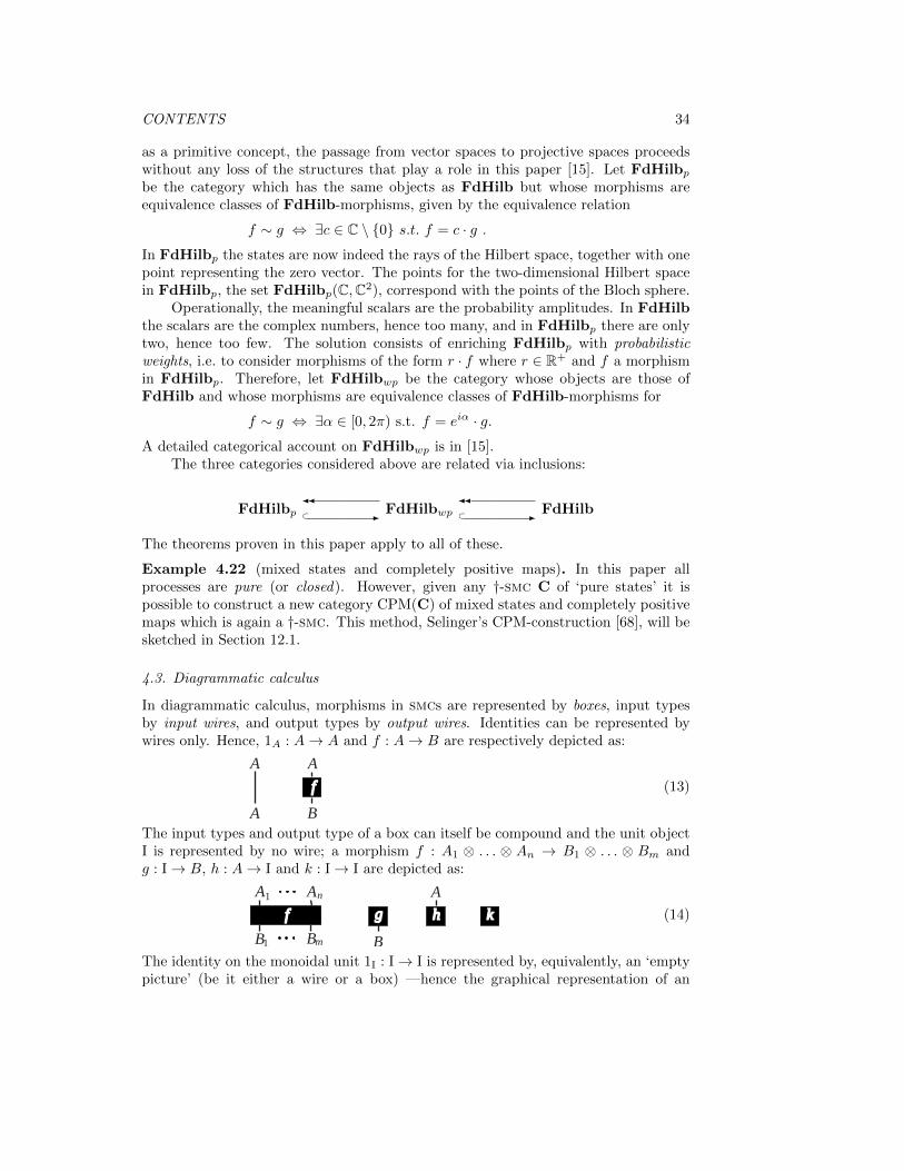
CONTENTS 34

as a primitive concept, the passage from vector spaces to projective spaces proceedswithout any loss of the structures that play a role in this paper [15]. Let FdHilbpbe the category which has the same objects as FdHilb but whose morphisms areequivalence classes of FdHilb-morphisms, given by the equivalence relation

f ∼ g ⇔ ∃c ∈ C \ {0} s.t. f = c · g .In FdHilbp the states are now indeed the rays of the Hilbert space, together with onepoint representing the zero vector. The points for the two-dimensional Hilbert spacein FdHilbp, the set FdHilbp(C,C2), correspond with the points of the Bloch sphere.

Operationally, the meaningful scalars are the probability amplitudes. In FdHilbthe scalars are the complex numbers, hence too many, and in FdHilbp there are onlytwo, hence too few. The solution consists of enriching FdHilbp with probabilisticweights, i.e. to consider morphisms of the form r · f where r ∈ R+ and f a morphismin FdHilbp. Therefore, let FdHilbwp be the category whose objects are those ofFdHilb and whose morphisms are equivalence classes of FdHilb-morphisms for

f ∼ g ⇔ ∃α ∈ [0, 2π) s.t. f = eiα · g.A detailed categorical account on FdHilbwp is in [15].

The three categories considered above are related via inclusions:

FdHilbp��⊂ - FdHilbwp

��⊂ - FdHilb

The theorems proven in this paper apply to all of these.

Example 4.22 (mixed states and completely positive maps). In this paper allprocesses are pure (or closed). However, given any †-smc C of ‘pure states’ it ispossible to construct a new category CPM(C) of mixed states and completely positivemaps which is again a †-smc. This method, Selinger’s CPM-construction [68], will besketched in Section 12.1.

4.3. Diagrammatic calculus

In diagrammatic calculus, morphisms in smcs are represented by boxes, input typesby input wires, and output types by output wires. Identities can be represented bywires only. Hence, 1A : A→ A and f : A→ B are respectively depicted as:

f

A

B

A

A

(13)

The input types and output type of a box can itself be compound and the unit objectI is represented by no wire; a morphism f : A1 ⊗ . . . ⊗ An → B1 ⊗ . . . ⊗ Bm andg : I→ B, h : A→ I and k : I→ I are depicted as:

f

A

B

A

B

1

1

n

m B

g h

A

k (14)

The identity on the monoidal unit 1I : I→ I is represented by, equivalently, an ‘emptypicture’ (be it either a wire or a box) —hence the graphical representation of an

CONTENTS 35

equation of the form s = 1I leaves the right-hand side empty. The symmetry naturalisomorphisms σA,B : A⊗B ' B ⊗A are depicted as:

A

BA

B

(15)

These boxes††, straight wires, and crossings of wires are the only graphical elementsthat make up the graphical language. We can compose morphisms in an smcin two manners, and similarly, we can compose these graphical elements in twomanners, depicted by connecting matching outputs and inputs by wires, and tensorby juxtaposing wires or boxes side by side. Hence g ◦ f : A → B → C andf ⊗ g : A⊗ C → B ⊗D are respectively depicted as:

f

C

g

A

B

f

A

D

g

C(16)

where A,B,C,D may themselves be compound as in (14). Morphisms that play specialroles may of course be given special graphical representations, sometimes other thanboxes. The connection between this graphical language and the symbolic definition ofsmcs is established as follows.

Definition 4.23. By isomorphism of diagrams we mean that there is a bijectivecorrespondence between boxes and wires which preserves the manner in which boxesand wires are connected —symmetry (cf. 15) is interpreted as a pair of crossing wires.

We will use equality “=” to denote isomorphic diagrams. Examples are:

= =A C A C A C A C

B D B D D B D B

f

g fg

f

fg

g(17)

Each represents (part of) an axiom of smcs, namely commutation of:

A⊗ C1A⊗g //

f⊗1C��

A⊗D

f⊗1D��

A⊗ CσA,C //

f⊗g��

C ⊗A

g⊗f��

B ⊗ C1B⊗g

// B ⊗D B ⊗D σB,D// D ⊗B

(18)

This correspondence instantiates a perfect correspondence between the symbolicrepresentation and the graphical presentation of smcs:

Theorem 4.24 (Joyal-Street [47]). An equation expressed in the symbolic languageof smcs follows from the axioms of smcs if and only if it holds up toisomorphism of diagrams in the graphical language.

††Although ‘box’ should be understood figuratively: we allow ourselves other shapes as well.

CONTENTS 36

As Selinger pointed out in [68], this result straightforwardly extends to †-smcs,when representing the adjoint by vertical reflection. This requires breaking thesymmetry of the boxes used above, and f : A → B and f† : B → A will now berespectively depicted as:

B A

BAf f (19)

Note that reflecting twice leaves the box invariant, exposing the involutive nature ofthe adjoint.

4.4. Graphical reasoning

In the following sections the graphical language will be preferred to conventional linearsyntax. Before proceding, we briefly discuss the question of equational reasoningin the graphical language: when do two diagrams denote the same mathematicalobject? When are two diagrams equal? There are two basic elements: isomorphismof diagrams, as discussed above; and substitution. Together these principles allow usto reason by rewriting.

The first prinicple, isomorphism, requires little elaboration beyond the discussionof Section 4.3. The graphical language is a syntax for describing certain mathematicalobjects, namely the arrows of symmetric monoidal categories; Theorem 4.24 statesthat two diagrams denote equal arrows when they are isomorphic (in the sense ofDefinition 4.23) .

However, the axioms of smcs are rather weak, so the isomorphism principle willnot suffice. We must impose other equations upon our diagrams to obtain our results.For example, consider an arrow f : A → A. The statement that f is unitary isexpressed by the equations

f ◦ f† = 1A = f† ◦ f . (20)

Since this equation is a property of the particular morphism f , there is no hopeto absorb it into some overarching global principle, in the way that Theorem 4.24absorbs the axioms of smcs. Indeed, most of the equations in this paper are of thissort, naked identifications that must be imposed on the langauge. We deal with thesevia substitution.

From a syntactic point of view, the meaning of an equation such as (20) is thatwhenever f† ◦ f is found lurking inside some larger expression, it can be replaced by1A without changing the meaning of the containing expression. The same method ofsubstitution applies in the graphical language.

The equations above can be easily translated into diagrams:

f

f= =

f

f

To perform the substitution, we isolate the part of the diagram corresponding to oneside of the equation, and form a new diagram by replacing that part with the other

CONTENTS 37

side of the equation.

f

f

g

=

g

Since two equal diagrams must have the same type, such a replacement is alwayspossible.

In general, when presented with a diagram d, any vertical line (which does notintersect any box or wire) divides the diagram into two parts, f and g, each of whichis a valid diagram, and which are related by the equation d = f ⊗ g. Similarly,any horizontal line (which may cut wires, but avoids boxes and points where wirescross) will divide d into two sub-diagrams, f ′ and g′, which satisfy d = f ′ ◦ g′. By asequence of such horizontal and vertical divisions, the diagram can be cut into squareseach of which contains an atomic element of the graphical language: a single box,a single crossing of wires, or a single straight wire. Each atomic square correspondsa single symbol in standard notation, and hence the factorisation yields a symbolicexpression equivalent to the diagram. The desired substitution can be performed onthe symbolic expression, and a new diagram constructed. We can pass freely from thesymbolic representation to the graphical representation and back.

f

f

g

=

g

(1A ⊗ g) ◦ (σ ⊗ (f† ◦ f))?

= (1A ⊗ g) ◦ (σ ⊗ 1A)

6

The above justification for substitution is admittedly rather sketchy. Joyal and Street[47] provide rigorous presentation with all the details. In practice, there is no need todivide a diagram into atomic pieces: it suffices to isolate the part to be substituted.We will apply this technique throughout this paper.

4.5. Correctness of graphical reasoning in zx-calculus

The cautious reader will be aware that the T-rule of the zx-calculus in Section 2—‘onlythe topology of the diagram matters’—stretches well beyond the graphical reasoningtechniques outlined above. As well as being a †-smc, ZX has a richer structure, andenjoys a correspondingly stronger analogue to Theorem 4.24.

Definition 4.25. A dagger compact (closed) category is a †-smc in which for eachobject A there exists dual object A∗ and a morphism ηA : I → A∗ ⊗ A subject tocertain coherence equations (for which see [1, 68]).

Throughout this paper we will take A∗ = A; this self-duality requires someadditional coherence axioms for which we refer the reader to [70].

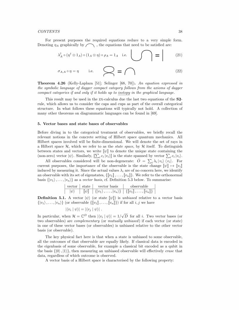
CONTENTS 38

For present purposes the required equations reduce to a very simple form.Denoting ηA graphically by , the equations that need to be satisfied are:

λ†A ◦ (η† ⊗ 1A) ◦ (1A ⊗ η) ◦ ρA = 1A i.e. (21)

σA,A ◦ η = η i.e. (22)

Theorem 4.26 (Kelly-Laplaza [51]; Selinger [68, 70]). An equation expressed inthe symbolic language of dagger compact category follows from the axioms of daggercompact categories if and only if it holds up to isotopy in the graphical language.

This result may be used in the zx-calculus due the last two equations of the S2-rule, which allows us to consider the caps and cups as part of the overall categoricalstructure. In what follows these equations will typically not hold. A collection ofmany other theorems on diagrammatic languages can be found in [69].

5. Vector bases and state bases of observables

Before diving in to the categorical treatment of observables, we briefly recall therelevant notions in the concrete setting of Hilbert space quantum mechanics. AllHilbert spaces involved will be finite-dimensional. We will denote the set of rays ina Hilbert space H, which we refer to as the state space, by H itself. To distinguishbetween states and vectors, we write JψK to denote the unique state containing the(non-zero) vector |ψ〉. Similarly, J

∑i ci |vi〉K is the state spanned by vector

∑i ci |vi〉.

All observables considered will be non-degenerate: O =∑i λi |vi〉 〈vi| . For

current purposes, the importance of the observable is the state change JψK 7→ JviKinduced by measuring it. Since the actual values λi are of no concern here, we identifyan observable with its set of eigenstates, {Jv1K , . . . , JvnK}. We refer to the orthonormalbasis {|v1〉 , . . . , |vn〉} as a vector basis, cf. Definition 5.3 below. To summarise:

vector state vector basis observable|ψ〉 JψK {|v1〉 , . . . , |vn〉} {Jv1K , . . . , JvnK}

Definition 5.1. A vector |ψ〉 (or state JψK) is unbiased relative to a vector basis{|v1〉 , . . . , |vn〉} (or observable {Jv1K , . . . , JvnK}) if for all i, j we have

|〈vi | ψ〉| = |〈vj | ψ〉| .

In particular, when H = CD then |〈vi | ψ〉| = 1/√D for all i. Two vector bases (or

two observables) are complementary (or mutually unbiased) if each vector (or state)in one of these vector bases (or observables) is unbiased relative to the other vectorbasis (or observable).

The key physical fact here is that when a state is unbiased to some observable,all the outcomes of that observable are equally likely. If classical data is encoded inthe eigenbasis of some observable, for example a classical bit encoded as a qubit inthe basis {|0〉 , |1〉}, then measuring an unbiased observable will effectively erase thatdata, regardless of which outcome is observed.

A vector basis of a Hilbert space is characterised by the following property:

CONTENTS 39

Proposition 5.2. Let {|v1〉 , . . . , |vn〉} be any vector basis of a Hilbert space H. Then,any linear map f : H → H′ is completely determined by the values f takes on|v1〉 , . . . , |vn〉. Further, no proper subset {|v1〉 , . . . , |vn〉} suffices to determine f .

Any regular linear map induces a map from states to states, namely

f :: JψK 7→ Jf(|ψ〉)K .

However, the values that f takes on an observable {Jv1K , . . . , JvnK} do not suffice to

fix f itself. For example, let θ, θ′ ∈ [0, 2π), and define a family of linear maps, relativeto basis {|0〉 , |1〉}, by the matrix:

fθ =

(1 00 eiθ

).

Every fθ leaves both |0〉 and |1〉 invariant, while

f(J+K) =q|0〉+ eiθ |1〉

y6=

r|0〉+ eiθ

′|1〉

z= fθ′(J+K)

whenever θ 6= θ′. Is there an analogue to Proposition 5.2? Can f be characterised byits image on some minimal set of states? The answer is yes:

Definition 5.3. A set of states of the form

observable ∪ {unbiased state for that observable}is called a state basis. The unbiased state is called the erasing point.

Proposition 5.4. Any map on states f induced by a regular linear map f : H → H′is completely determined by the values it takes on a state basis for some arbitraryobservable. Moreover, no proper subset of such a set of states suffices to determine f .

Proof. Let f be a regular linear map, and let f be the corresponding map of states.Let {Jv1K , . . . , JvnK}∪{JsK} form a state basis, and suppose that f takes known valuesupon these states. We will show this determines f on a vector basis {|η1〉 , . . . , |ηn〉}of H, up to a common, overall phase.

Set |ηi〉 = 〈vi | s〉 |vi〉 and let H′′ be the subspace spanned by f(|η1〉), . . . , f(|ηn〉).Since f is regular {f(|η1〉), . . . , f(|ηn〉)} is a basis for H′′, and let 〈− | −〉� denotethe inner-product on H′′ for which {f(|η1〉), . . . , f(|ηn〉)} is orthonormal. Then thecodomain restriction of f to (H′′, 〈− | −〉�) is unitary. Relying on this we havef(|ηi〉) = f(〈vi | s〉 |vi〉) = 〈vi | s〉f(|vi〉) = 〈f(|vi〉) | f(|s〉)〉� f(|vi〉). This expression

is completely determined by f(JviK) and f(JsK) up to a phase factor contributed byf(|s〉), but this phase factor is the same for all f(|ηi〉).

It now follows that, given an arbitary state JψK = J∑i ci |ηi〉K, we have f(JψK) =

Jf(|ψ〉)K = Jf(∑i ci |ηi〉)K = J

∑i cif(|ηi〉)K, where each f(|ηi〉) is determined upto the

common phase. This phase is therefore a global phase for the vector∑i cif(|ηi〉),

hence f(JψK) yields a unique state, and so f is well-defined on all states.It is easily seen that no proper subset of {Jv1K , . . . , JvnK , JsK} is sufficient to

completely determine f . 2

State bases and vector bases are related by the following proposition:

Proposition 5.5. Let S be the set of all state bases for H, let V be the set of allvector bases for H, and let V/ ∼ be the set of equivalence classes [−]∼ in V for theequivalence relation ‘equal up to an overall phase’ i.e.

CONTENTS 40

{|v1〉 , . . . , |vn〉} ∼ {|w1〉 , . . . , |wn〉} ⇔ ∃θsuch that ∀j : |vj〉 = eiθ · |wj〉 .There is a bijective correspondence

Ssv -- V/ ∼vs

ll

where

• sv : {Jv1K , . . . , JvnK} ∪ {JsK} 7→ [{〈v1 | s〉 |v1〉 , . . . , 〈vn | s〉 |vn〉}]∼• vs : [{|v1〉 , . . . , |vn〉}]∼ 7→ {Jv1K , . . . , JvnK} ∪ {J

∑i |vi〉K}.

Proof. Note that sv is indeed well-defined in the sense that its prescription doesnot depend on the choice of the respective vectors |v1〉 , . . . , |vn〉 , |s〉 in the statesJv1K , . . . , JvnK , JsK. Also vs is easily seen to be well-defined. Verifying that thesemaps are each other’s inverse is straightforward. 2

Example 5.6. On the Bloch sphere the erasing point lies on the equator for theantipodal points that represent the observable. E.g. for the Z-observable {J0K , J1K}and the erasing point J+K := J|0〉+ |1〉K we have:

so the observable and the erasing point together make up a T-shape.

Given a vector basis, we can turn it into an observable by forgetting the phasesof each of the basis vectors, which we formalise by passing to equivalence classes. Toconstruct a vector basis from an observable, we have to choose a phase for each basiselement. This construction factors over the construction of state bases as follows:

observablechoose erasing point ..

choose individual phases

**state basis

forget erasing pointnn Prop. 5.5

choose overall phase..vector basis

forget overall phase

nn

forget individual phases

jj

Definition 5.7. A pair of mutually unbiased vector bases (MUVBs), V ={|v1〉 , . . . , |vn〉} and W = {|w1〉 , . . . , |wn〉}, are called coherent iff

1√n

∑i

vi ∈ W ,1√n

∑i

wi ∈ V .

Two mutually unbiased state bases (MUSBs) are coherent iff the erasing point of eachis contained in the observable of the other.

These notions of coherence coincide along the bijection of Proposition 5.5:

Proposition 5.8. If V and W are coherent MUVBs then vs([V]∼) and vs([W]∼) arecoherent MUSBs, and if S and T are coherent MUSBs then there exist V ∈ sv(S) andW ∈ sv(T ) such that V and W are coherent MUVBs.

CONTENTS 41

Proof. The first statement follows directly from the definition of vs. Let S ={Jv1K , . . . , JvnK , Jw1K} and T = {Jw1K , . . . , JwnK , Jv1K} be coherent MUSBs; forV ∈ sv(S) and W ∈ sv(T ) we have

∑i V =

∑i〈vi | w1〉 |vi〉 = |w1〉 and

∑iW = |v1〉.

Hence we obtain coherence if 〈w1 | v1〉 |w1〉 = |w1〉 and 〈v1 | w1〉 |v1〉 = |v1〉, that is,〈v1 | w1〉 = 1. This can be realised by choosing an appropriate overall phase for Vrelative to W. 2

Pairs of observables arise from coherent bases:

Theorem 5.9. For each pair of MUVBs {|v1〉 , . . . , |vn〉} and {|w1〉 , . . . , |wn〉} thereexists a pair of coherent MUVBs {|v′1〉 , . . . , |v′n〉} and {|w′1〉 , . . . , |w′n〉} that inducesthe same observables i.e. JviK = Jv′iK and JwiK = Jw′iK for all i.

Proof. Given a pair of MUVBs forget all phases to obtain the corresponding pair ofinduced observables. Then adjoin as an erasing point to each of these a state of theother, in order to obtain coherent MUSBs. Now we can rely on Proposition 5.8 toobtain coherent MUVBs that induce the same observable as the initial one. 2

6. Algebras and observables

In the introduction of this paper we already indicated how conceptual analysis leadsto an algebraic characterization of bases and observables. Here we review this theoryin technical detail. Its main purpose is a characterization of bases in the language of †-smcs—i.e. with no reference to vectors, sums, linear combinations etc. —allowing basesto be defined in purely diagrammatic terms. As we shall also see, the diagrammaticpresentation of bases admits very simple calculational rules in terms of so-called‘spiders’— indeed, those that play a central role in the zx-calculus.

6.1. Monoids, comonoids, and observable structures

Recall that a monoid is a triple (M, •, 1•) with M a set, • an associative multiplication,and 1• ∈M is its unit. The multiplication is a map:

m• : M ×M →M :: (x, y) 7→ x • y (23)

and we can also represent the unit as a map

e• : I→M :: ? 7→ 1• (24)

where I := {?} is a singleton set. The associativity and unit laws of the monoid cannow be re-written in terms of composition of maps and cartesian product:

m• ◦ (m• × 1M ) = m• ◦ (1M ×m•) , (25)

m• ◦ (e• × 1M ) ' m• ◦ (1M × e•) ' 1M (26)

where 1M : M →M is the identity map on M . Now, (M,m•, e•) is commutative if

m• ◦ σM,M = m• (27)

where σM,M : (x, y) 7→ (y, x).More generally, commutative monoids can be defined internally in any smc.

CONTENTS 42

Definition 6.1. An internal commutative monoid in an smc is a triple (M,m, e),consisting of an object M , equipped with a multiplication m : M ⊗M → M , and aunit e : I→M , satisfying

m ◦ (m⊗ 1M ) = m ◦ (1M ⊗m) , (28)

m ◦ (e⊗ 1M ) ◦ λM = m ◦ (1M ⊗ e) ◦ ρM = 1M , (29)

m ◦ σM,M = m. (30)

By reversing the types and the order of composition we obtain a new concept.

Definition 6.2. An internal cocommutative comonoid in an smc is a triple (X, δ, ε)consisting of an object X equipped with a comultiplication δ : X → X ⊗ X and acounit ε : X → I, satisfying

(δ ⊗ 1X) ◦ δ = (1X ⊗ δ) ◦ δ , (31)

λ−1X ◦ (ε⊗ 1X) ◦ δ = ρ−1X ◦ (1X ⊗ ε) ◦ δ = 1X , (32)

σX,X ◦ δ = δ . (33)

Note that in a †−smc each internal commutative monoid is also an internalcocommutative comonoid, for δ := m† and ε := e†, and vice versa.

Now consider a set X and let δ : X → X×X be the function which copies entries,i.e. δ :: x 7→ (x, x). Since δ is a function it is also a relation, namely

δ := {(x, (x, x)) | x ∈ X} ⊆ (X ×X)×X , (34)

and as a relation it admits a relational converse, obtained by exchanging the twoentries in the pairs which make up that relation. The relational converse to δ,

m := {((x, x), x) | x ∈ X} ⊆ (X ×X)×X , (35)

relates pairs (x, x) ∈ X×X to x ∈ X, while it does not relate pairs (x, y) ∈ X×X forx 6= y to anything. Let ε : X → I be the function which erases entries i.e. ε : x 7→ ?.When conceived as a relation ε admits a relational converse

e := {(?, x) | x ∈ X} ⊆ I×X , (36)

which now relates ? ∈ I to each x ∈ X. The copying/erasing pair (δ, ε) is a comonoidin Rel, and the pair (m, e) consisting of their respective converses is a monoid in Rel.The pair (m, δ) moreover satisfies another remarkable property:

δ ◦m = (1X ×m) ◦ (δ × 1X) = {(x, x), (x, x) | x ∈ X} . (37)

Remark 6.3. This interesting property first appeared in the literature as part ofCarboni and Walters’ axiomatisation of the category Rel in [12] where they introducedthe notion of a Frobenius algebra in an smc C, as a quintuple of morphisms

(X, d : X ⊗X → X, e : I→ X, δ : X → X ⊗X, ε : X → I) (38)

where (X,m, e) is an internal commutative monoid and (X, δ, ε) is an internalcocommutative comonoid, which together satisfy the Frobenius law— see (40) below.

Definition 6.4. [27] An observable structure in a †-smc is a triple(A , δ = : A→ A⊗A , ε = : A→ I

)which:

CONTENTS 43

(i) is a cocommutative comonoid; the defining equations (31,32,33) are depicted as:

(39)

(ii) satisfies the Frobenius law, that is,

(δ† ⊗ 1A) ◦ (1A ⊗ δ) = δ ◦ δ† i.e. (40)

(iii) is special, that is,

δ† ◦ δ = 1A i.e. . (41)

Example 6.5. The unit object I canonically comes with an observable structure:

δI := λI : I ' I⊗ I , εI := 1I . (42)

Example 6.6. As indicated in the introduction to this paper, any orthonormal basis{|ψi〉}i for a Hilbert space H induces an observable structure by considering the linearmaps that respectively ‘copy’ and ‘uniformly erase’ the basis vectors:

δ : H → H⊗H :: |ψi〉 7→ |ψi〉 ⊗ |ψi〉 , ε : H → C :: |ψi〉 7→ 1 . (43)

Moreover, this observable structure is ‘basis capturing’: we can recover the basisvectors from which we constructed δ as the solutions to the equation

δ(|ψ〉) = |ψ〉 ⊗ |ψ〉 . (44)

This also shows that the basis {|ψi〉}i is faithfully encoded in the linear map δ alone,and that ε does not carry any additional data.

Conversely, all observable structures in FdHilb arise from bases:

Theorem 6.7. [28] All observable structures in FdHilb are of the form (43).

So observable structures provide an axiomatic characterisation of bases in †-smc-language, with no reference to the linear structure of the underlying vector spaces.

Example 6.8. Each observable structure in FdHilb induces an observable structurein FdHilbwp in the obvious manner. But, in the light of Proposition 5.5, thecorrespondence in FdHilb between observable structures and vector bases, becomesone between observable structures and state bases in FdHilbwp. Note that

δ : H → H⊗H :: JψiK 7→ J|ψi〉 ⊗ |ψi〉K (45)

does not define a unique δ anymore. In addition we need to specify that J∑i |ψi〉K,

the erasing point of the state basis, provides the unit for the comultiplication:

δ†

(−⊗

t∑i

|ψi〉

|)= 1H . (46)

Corollary 6.9. Observable structures in FdHilbwp are in bijective correspondencewith state bases via the correspondence outlined in Example 6.8.

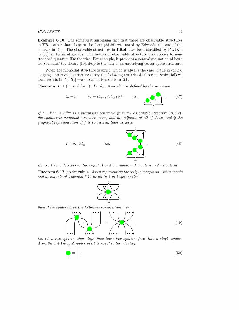
CONTENTS 44

Example 6.10. The somewhat surprising fact that there are observable structuresin FRel other than those of the form (35,36) was noted by Edwards and one of theauthors in [19]. The observable structures in FRel have been classified by Pavlovicin [60], in terms of groups. The notion of observable structure also applies to non-standard quantum-like theories. For example, it provides a generalised notion of basisfor Spekkens’ toy theory [19], despite the lack of an underlying vector space structure.

When the monoidal structure is strict, which is always the case in the graphicallanguage, observable structures obey the following remarkable theorem, which followsfrom results in [53, 54] —a direct derivation is in [23].

Theorem 6.11 (normal form). Let δn : A→ A⊗n be defined by the recursion

δ0 = ε , δn = (δn−1 ⊗ 1A) ◦ δ i.e. ︸ ︷︷ ︸n

. (47)

If f : A⊗n → A⊗m is a morphism generated from the observable structure (A, δ, ε),the symmetric monoidal structure maps, and the adjoints of all of these, and if thegraphical representation of f is connected, then we have

f = δm ◦ δ†n i.e.

n︷ ︸︸ ︷

︸ ︷︷ ︸m

. (48)

Hence, f only depends on the object A and the number of inputs n and outputs m.

Theorem 6.12 (spider rules). When representing the unique morphism with n inputsand m outputs of Theorem 6.11 as an ‘n+m-legged spider’:

n︷ ︸︸ ︷︸ ︷︷ ︸

m

,

then these spiders obey the following composition rule:

. (49)

i.e. when two spiders ‘share legs’ then these two spiders ‘fuse’ into a single spider.Also, the 1 + 1-legged spider must be equal to the identity:

, (50)

CONTENTS 45

and thirdly, spiders are invariant under ‘leg swapping’:

. (51)

Conversely, given a family {δ†m ◦ δn|n,m ∈ N} of morphisms, the equations definingan observable structure can be recovered from (49), (50) and (51), hence providing analternative characterization of observable structures now purely in terms of spiders.

Example 6.13. We have:

(1A ⊗ δ†2) ◦ (δ2 ⊗ δ2) ◦ (1A ⊗ σA,A ⊗ 1A) ◦ (δ†2 ⊗ δ†2) ◦ (δ2 ⊗ 1A)

= = δ3 ◦ δ†3.

The spider rules enabled us to define the zx-calculus of section 2 in terms of spidersobeying the rules (49) and (50), rather than algebras. The swapping of remainingrule (51) was eliminated by (implicitly) allowing freedom of how to spiders may beconnected, absorbing the symmetry into the graph structure (see Example 2.3). Herewe have been more explicit. The angles labeling the spiders of the zx-calculus will beexplained below in Section 7.

6.2. Induced †-compact structure

Definition 6.14. A self-dual †-compact structure is a pair

(A, η : I→ A⊗A)

which satisfies equations (21) and (22).

Proposition 6.15. Every observable structure on an object A defines a self-dual †-compact structure when setting η = δ02.

Proof. Equations (21) and (22) follow from equations (49) and (51) respectively. 2

Remark 6.16. The †-compact structures induced by different observable structuresmay or may not coincide [26]. For example, while †-compact structures induced by theobservable structures that copy the {|0〉 , |1〉} and {|+〉 , |−〉} coincide, this is not thecase for the bases {|0〉 , |1〉} and {|0〉+ i |1〉 , |0〉 − i |1〉}. Returning to the zx-calculus,the two equations of the S2-rule are quite different to each other. The equations

are true because of the counit law for the observable structure, and the fact there isonly one identity map. On the other hand the equations

CONTENTS 46

are not a consequence of the axioms of an observable structure, but a fact specific tothe Z and X bases. Only when no confusion is possible we simplify the notation forthe 0 + 2-legged spider, as in the zx-calculus:

.

The dots will be retained when disambiguation is required.

Definition 6.17. Let f : A→ B be a morphism. Its transpose, f∗ : B → A, and itsconjugate, f∗ : A→ B, relative to observables structures on A and B, are defined as:

f∗ := (1A ⊗ η†B) ◦ (1A ⊗ f ⊗ 1B) ◦ (ηA ⊗ 1B),

f∗ := (1B ⊗ η†A) ◦ (1B ⊗ f† ⊗ 1A) ◦ (ηB ⊗ 1A) .

Diagrammatically, we denote f∗ and f∗ respectively as:

A

B

B

A

ff f

A

A

B

B

f

The green squares indicate the dependency of f∗ and f∗ on the observable structureson A and B; when there is no risk of confusion we omit the colouration and rely simplyupon the position of the indicated corner to distinguish between f , f†, f∗, and f∗. Wefollow [68] in representing the conjugate by horizontal reflection and the transpose bya 180◦ rotation:

A A

BBf f

B B

AAf ff

f †

f*

f *

which is consistent with the fact that

f∗ = (f†)∗ = (f∗)† , or equivalently , f† = (f∗)∗ = (f∗)∗ .

Corollary 6.18. For an observable structure all spiders are self-conjugate.

Example 6.19. In FdHilb every observable structure corresponds to a basis, as perExample 6.6. The linear function f∗ is obtained by conjugating the entries of thematrix of f when expressed in the bases corresponding to the observable structureson A and B; f∗ is obtained by transposing the matrix of f .

Definition 6.20. Let A be an object in a †-smc which comes with an observablestructure, and hence an induced †-compact structure (A, η). The dimension of A isdim(A) := η† ◦ η, represented graphically by a circle:

Lemma 6.21. Dimension is independent of the choice of observable structure.

CONTENTS 47

Proof. We will depict the two distinct observable structures in green and redrespectively. Then, repeatedly relying on †-compactness we have:

so the circles induced by the two observable structures coincide. 2

Remark 6.22. In the language of †-compact categories, the circle is formed by takingthe trace of the identity morphism; in a finite dimensional Hilbert space this will alwaysgive the dimension, hence the terminology dimA.

6.3. Classical points and generalised bases

We now provide a category-theoretic counterpart to the role played by basisvectors/states in FdHilb and FdHilbwp.

Definition 6.23. Given an observable structure (A, δ, ε), a morphism k : I → A is aclassical point iff it is a self-conjugate comonoid homomorphism, that is, graphically:

k k (52)

k k k (53)

k(54)

Remark 6.24. The notation k reflects ‘sensitivity to conjugation’ while the

notation k reflects ‘invariance under conjugation’. We used k in (52) to express

invariance under conjugation, and given this fact, we used k in (53) and (54).

Proposition 6.25. Classical points are normalised.

Proof. Since each classical point k : I→ A is self-conjugate its adjoint k† : A→ I andits transpose k∗ : A→ I coincide. Hence we have:

k

k

k kk

k

that is, k† ◦ k = 1I. 2

CONTENTS 48

Example 6.26. In FdHilb the classical points for an observable structure are exactlythe basis vectors {|v1〉 , . . . , |vn〉} and in FdHilbwp they constitute the correspondingobservable {|v1〉 , . . . , |vn〉}. Hence, while in FdHilb the classical points completelydetermine an observable structure, this is not the case in FdHilbwp, where it is theclassical points together with an erasing point that determine an observable structure.

The following is a category-theoretic generalisation of a notion of basis, eitherin the sense of Proposition 5.2 or in the sense of Proposition 5.4, which respectivelyapplies to the categories FdHilb and FdHilbwp.

Definition 6.27. An observable structure (A, δ, ε) with classical points K is called avector basis iff for all objects B and all morphisms f, g : A→ B we have[

∀k ∈ K : f ◦ k = g ◦ k]⇒ f = g . (55)

It is called a state basis iff for all B and all f, g : A→ B we have[∀k ∈ K ∪ {ε†} : f ◦ k = g ◦ k

]⇒ f = g . (56)

One can easily construct new observable structures by combining old ones, as thein the following proposition.

Proposition 6.28. Two observable structures (A, δA, εA) and (B, δB , εB) canonicallyinduce an observable structure on A⊗B with

δA⊗B = (1A ⊗ σA,B ⊗ 1B) ◦ (δA ⊗ δB) i.e. A B , (57)

and

εA⊗B = λ†I ◦ (εA ⊗ εB) i.e. A B . (58)

Moreover, if k : I→ A is a classical point for (A, δA, εA) and k′ : I→ B is a classicalpoint for (B, δB , εB) then (k ⊗ k′) ◦ λI is a classical point for (A⊗B, δA⊗B , εA⊗B).

Definition 6.29. We say that the monoidal tensor lifts vector bases iff for all vectorbases (A, δA, εA) with classical points K and (B, δB , εB) with classical points K′, allobjects C, and all morphisms f, g : A⊗B → C, we have that[

∀(k, k′) ∈ K ×K′ : f ◦ (k ⊗ k′) = g ◦ (k ⊗ k′)]⇒ f = g . (59)

– hence it follows that the observable structure (A ⊗ B, δA⊗B , εA⊗B) is also vectorbasis. Similarly, the monoidal tensor lifts state bases iff[

∀(k, k′) ∈ (K ×K′) ∪ {(ε†A, ε†B)} : f ◦ (k ⊗ k′) = g ◦ (k ⊗ k′)

]⇒ f = g .(60)

– hence it follows that (A⊗B, δA⊗B , εA⊗B) is also state basis.

Since observable structures induce †-compact structures we have the following.

Proposition 6.30. Monoidal tensors always lift vector bases and state bases.

Proof. We have:

f

k k‘g

k k‘

⇔ f

k

k‘g

k

k‘∗⇔ f

k‘g

k‘

⇔ f

k‘

g

k‘

∗⇔ f g ⇔ f g

CONTENTS 49

where the marked equivalences rely on the vector/state basis assumption. 2

7. Phase shifts and a generalised spider theorem

In the preceding section we saw that observable structures correspond to bases of ourstate space; now we introduce an abstract notion of phase relative to a given basis,and generalise Theorems 6.11 and 6.12 to incorporate such phase shifts.

7.1. A monoid structure on points

Definition 7.1. Let (A, δ, ε) be an observable structure in a †-smc C and let C(I, A)be the underlying set of points. We define a multiplication on points

−�− : C(I, A)×C(I, A)→ C(I, A) (61)

by setting, for all points ψ, φ ∈ C(I, A),

ψ � φ := δ† ◦ (ψ ⊗ φ) ◦ λI i.e. . (62)

Remark 7.2. As already explained in Remark 6.24, the shape of the points reflectsthat they may not be invariant under conjugation.

Proposition 7.3. (C(I, A),�, ε†, (−)∗) is an involutive commutative monoid.

Proof. Associativity, commutativity, and that ε† is the monoid’s unit, i.e.:

θθ

follow immediately from internal monoid laws for (A, δ†, ε†)— see (39) above — andconjugutation is an involution since δ† is self-conjugate— see Corollary 6.18. 2

Example 7.4. Let δZ : C2 → C2 ⊗ C2 be defined by δ : |i〉 7→ |ii〉. The inducedmultiplication �Z is just point-wise multiplication in the standard basis:(

ab

)�Z

(a′

b′

)= δ†Z

((ab

)⊗(a′

b′

))=

(aa′

bb′

).

Indeed, the same will be true for any observable structure, provided we write thevectors in the corresponding basis.

As well as giving an involutive commutative monoid on the points of A, we canuse δ† to lift this monoid up to the endomorphisms of A.

Definition 7.5. For (A, δ, ε) an observable structure in a †-smc C let

Λ : C(I, A)→ C(A,A) (63)

be defined by setting, for each point ψ ∈ C(I, A),

Λ(ψ) = δ† ◦ (ψ ⊗ 1A) i.e. , (64)

and we denote the range of Λ by Λ(A,A).

CONTENTS 50

Proposition 7.6. The map Λ is an isomorphism of involutive commutative monoids:(C(I, A),�, ε†, (−)∗

)'(Λ(A,A), ◦, 1A, (−)†

). (65)

that is, explicitly:

Λ(ψ � φ) = Λ(ψ) ◦ Λ(φ) Λ(ε†) = 1A Λ(ψ∗) = Λ(ψ)†, (66)

and hence commutativity is inherited:

Λ(ψ) ◦ Λ(φ) = Λ(ψ � φ) = Λ(φ) ◦ Λ(ψ) i.e. . (67)

Proof. Preservation of monoid multiplication and unit follow directly from the unitand commutativity law of the internal monoid. By the spider rules we have:

that is, conjugation of points is mapped to the adjoint of endomorphisms. 2

Note that the notation of endomorphisms in Λ(A,A) is invariant under 180◦

rotations. This is justified by the following proposition.

Proposition 7.7. Each Λ(ψ) ∈ Λ(A,A) is equal to its transpose.

Proof. We have:

were we relied on the spider rules. 2

Proposition 7.8. The endomorphisms in Λ(A,A) obey

Λ(ψ) ◦ δ† = δ† ◦ (1A ⊗ Λ(ψ)) = δ† ◦ (Λ(ψ)⊗ 1A) (68)

i.e.

. (69)

Proof. By the spider rules all three diagrams normalise to:

so they are indeed all equal. 2

The following proposition shows that the inner-product structure on points issubsumed by the commutative involutive monoid structure on points.

Proposition 7.9. For points ψ, φ : I → A in C we have:

〈φ|ψ〉 := φ† ◦ ψ = ε ◦ (φ∗ � ψ) . (70)

CONTENTS 51

Proof. Using the definition of the transpose for φ† = (φ∗)∗ we obtain

*

where again we used the spider rules. 2

7.2. The decorated spider theorem

Theorem 7.10 (normal form with points). If f : A⊗n → A⊗m is a morphismgenerated from the observable structure (A, δ, ε), the symmetric monoidal structuremaps, and the adjoints of all of these, points ψi : I → A (exactly one occurrence foreach i), and if the graphical representation of f is connected then we have

f = δm ◦ Λ(⊙

i ψi

)◦ δ†n i.e.

n︷ ︸︸ ︷

︸ ︷︷ ︸m

.

Proof. If neither δ nor δ† occurs in f , then result is trivial. Otherwise, all points ψioccurring in f may be lifted to Λ(ψi); by virtue of Proposition 7.8, these commutefreely with the observable structure, hence can all be collected together. The resultnow follows by applying Theorem 6.11. 2

Theorem 7.10 is a strict generalisation of Theorem 6.11: diagrams with equalnumbers of inputs n and outputs m are equal whenever the product of points occurringin them is also equal. The theorem gives a specific normal form to which this entireclass of diagrams is equal; we also have corresponding decorated spider rules.

Theorem 7.11 (decorated spider rules). When setting

then these decorated spiders obey the following composition rule:

.

CONTENTS 52

i.e. when two decorated spiders ‘share legs’ then these two spiders ‘fuse’ together intoa single decorated spider provided we ‘multiply decorations’.

This is of course the form of the spider rule in the zx-calculus.

7.3. Unbiased points

Example 7.12. Let (δ, ε) be the observable structure corresponding to the standardbasis of Cn, and consider |ψ〉 =

∑i ci| i 〉. When written in the basis fixed by (δ, ε),

Λ(ψ) consists of the diagonal n × n matrix with c1, . . . , cn on the diagonal. Hence,Λ(ψ) is unitary if and only if c1c1 = . . . = cncn = 1, that is, if and only if |ψ〉 isunbiased for {|1〉 , . . . , |n〉} (upto a normalising constant).

This situation admits generalisation to arbitrary †-smcs.

Definition 7.13. We call a point α : I → A unbiased relative to an observablestructure (A, δ, ε) if there exists a scalar s : I→ I such that:

s · α� α∗ = ε† i.e.αα

s . (71)

Example 7.14. Since by the spider rules the point ε† satisfies this definition, everyobservable structure has at least one unbiased point, namely its unit.

Lemma 7.15. If an unbiased point α is normalised, i.e. α† ◦ α = 1I , then thescalar s in the above definition is equal to D = dimA. Hence, if on the other hand|α|2 := α† ◦ α = D then this scalar is 1I.

Proof. We have:

α α α

αs s s

where we relied on Proposition 7.9. 2

The expression α � α∗ denotes ‘convolution’ of α with itself; since the point ε†

represents the uniform distribution over the basis defining δ, this definition indeedcaptures the usual understanding of what it means for a vector to be unbiased withrespect to a basis. The following shows that this is exactly correct.

Lemma 7.16. Let α, k : I→ A be points of A such that α is unbiased and normalised,and k is classical, for (A, δ, ε); then

D · |〈k|α〉|2 := D · (k† ◦ α) · (α† ◦ k) = 1I i.e.α

αk

k. (72)

Proof. We have:

αα α α

α αk

k k k k k

where we relied on the fact that scalars are always self-transpose, used (53), used theadjoint to the unbiasedness law, and finally used (54). 2

CONTENTS 53

Remark 7.17. To retrieve the usual definition of unbiasedness,

|〈z | α〉| = 1√dimA

, (73)

we simply divide; however, since we operate in an arbitrary †-smc, the scalars form acommutative monoid rather than a group, so dividing is not always possible. Hencethe form (72) for the unbiasedness law.

7.4. The phase group

Proposition 7.18. A point α of length |α|2 = D is unbiased iff Λ(α) is unitary.

Proof. Due the commutativity property of Λ in Proposition 7.6 we need check onlyone equation to show that Λ(α) is unitary, namely,

Λ(α) ◦ Λ(α)† = 1A i.e.αα

. (74)

Suppose that α is unbiased; then by the spider rules we have

αααα

,

as required. The other direction of the proof is essentially the same. 2

Since unitary maps are invertible, they form a group, and this group structuretransfers back onto the unbiased points.

Theorem 7.19. If in the isomorphism of involutive commutative monoids ofProposition 7.6 we restrict ourselves to unbiased points relative to the observablestructure of length |α|2 = D, and unitary endomorphisms, then we obtain anisomorphism of abelian groups, with the involution as the inverse.

Proof. This immediately follows from Proposition 7.18 and the fact that for a unitarymorphism the adjoint is the inverse. 2

Definition 7.20. The abelian group of endomorphisms of Theorem 7.19 is called thephase group, and its elements are called phase shifts.

Remark 7.21. We chose |α|2 = D since this results in the inverse taking a simpleform; fixing another length would also have given us an abelian group structure.

Example 7.22. Consider the observable structure (C2, δZ , εZ) in FdHilb, defined by

δZ : |i〉 7→ |ii〉 , εZ : |0〉+ |1〉 7→ 1 .

Its classical points are {|0〉 , |1〉}. The unbiased points for (C2, δZ , εZ) are of the form|αZ〉 = |0〉 + eiα |1〉, and |αZ〉 �Z |βZ〉 = |(α+ β)Z〉, hence the group of unbiasedpoints is isomorphic to the interval [0, 2π) under addition modulo 2π. We have

ΛZ(α) =

(1 00 eiα

),

CONTENTS 54

and in particular, ΛZ(π) = Z. In other words, the phase shifts of the observablestructure are obtained by rotating along the equator of the Bloch sphere:

α.

In particular, we have |θ1〉�|θ2〉 = |θ1+ θ2〉, that is, the operation � is simply additionmodulo 2π, which is an abelian group with minus as inverse. This group of phasesplayed a key role in proving universality of the zx-calculus in Section 2.4.

Example 7.23. Phase groups can provide an algebraic witness for physical differencesbetween theories. For example, as shown in [20], the toy model category Spek (cf.Example 4.20) and the category Stab (a restriction of FdHilb to the qubit stabilizerstates) are essentially the same except for the phase groups of their respective qubits.In the case of Spek the phase group is the Klein four group Z2 × Z2, while for Stabthe phase group is the cyclic four group Z4. This difference in phase groups is closelyconnected to the fact that while states in Spek always admit a local hidden variablerepresentation, in Stab there are states which don’t, namely the GHZ state [58].

Example 7.24. Using decorated spider notation we can set

α :=(Λ(α)⊗ Λ(α)

)◦ δ ◦ Λ(α)† and α := ε ◦ Λ(α)†,

and for α unbiased relative to (A, δ, ε), again by the decorated spider rules, it followsthat these morphisms define an observable structure. Hence, each element of the phasegroup transforms the given observable structure into a new observable structure.

8. Complementarity is equivalent to the Hopf law

For observable structures (A, δZ , εZ) and (A, δX , εX) in a †-smc we will denote thecorresponding induced †-compact structures respectively as (A, ηZ) and (A, ηX). Firstwe study complementarity for pairs of observable structures on the same object withcoinciding induced †-compact structures, and then we study the slightly more involvedcase of non-coinciding induced †-compact structures— cf. Remark 6.16.

8.1. Observable structures with coinciding †-compact structures

First we define complementarity for observable structures in arbitrary †-smcs in amanner which makes explicit reference to their classical points, simply in analogywith the usual definition in Hilbert space quantum theory, and then we show that thisdefinition can be equivalently restated without any reference to points.

Definition 8.1. Two observable structures (A, δZ , εZ) and (A, δX , εX) in a †-smc arecalled complementary if they obey the following rules:

comp1 whenever z : I → A is classical for (δZ , εZ) it is unbiased for (δX , εX) ;

comp2 whenever x : I → A is classical for (δX , εX) it is unbiased for (δZ , εZ) .

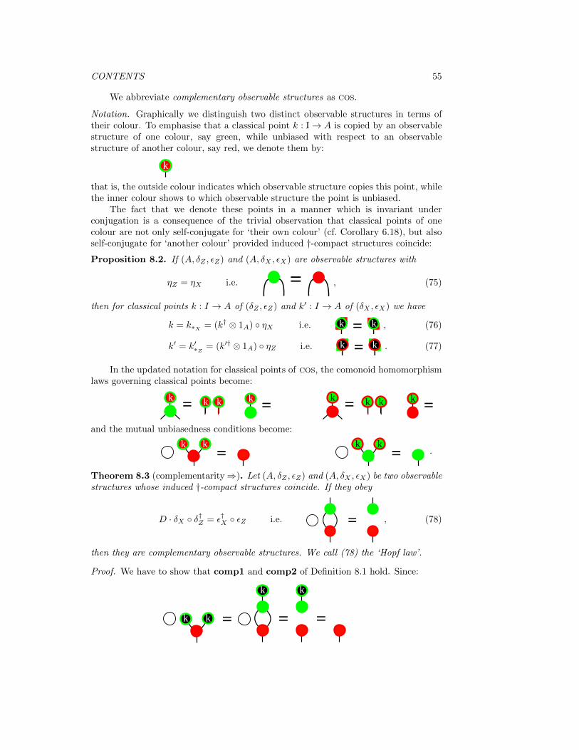
CONTENTS 55

We abbreviate complementary observable structures as cos.

Notation. Graphically we distinguish two distinct observable structures in terms oftheir colour. To emphasise that a classical point k : I→ A is copied by an observablestructure of one colour, say green, while unbiased with respect to an observablestructure of another colour, say red, we denote them by:

k

that is, the outside colour indicates which observable structure copies this point, whilethe inner colour shows to which observable structure the point is unbiased.

The fact that we denote these points in a manner which is invariant underconjugation is a consequence of the trivial observation that classical points of onecolour are not only self-conjugate for ‘their own colour’ (cf. Corollary 6.18), but alsoself-conjugate for ‘another colour’ provided induced †-compact structures coincide:

Proposition 8.2. If (A, δZ , εZ) and (A, δX , εX) are observable structures with

ηZ = ηX i.e. , (75)

then for classical points k : I → A of (δZ , εZ) and k′ : I → A of (δX , εX) we have

k = k∗X = (k† ⊗ 1A) ◦ ηX i.e. k k , (76)

k′ = k′∗Z = (k′† ⊗ 1A) ◦ ηZ i.e. k k . (77)

In the updated notation for classical points of cos, the comonoid homomorphismlaws governing classical points become:

k k k k k k k k

and the mutual unbiasedness conditions become:

kk kk.

Theorem 8.3 (complementarity⇒). Let (A, δZ , εZ) and (A, δX , εX) be two observablestructures whose induced †-compact structures coincide. If they obey

D · δX ◦ δ†Z = ε†X ◦ εZ i.e. , (78)

then they are complementary observable structures. We call (78) the ‘Hopf law’.

Proof. We have to show that comp1 and comp2 of Definition 8.1 hold. Since:

k k

k k

CONTENTS 56

comp1 holds; by exchanging the colours we obtain comp2. 2

The converse to Theorem 8.3 also holds if one of the observable structures involvedis either a vector or state basis— cf. Definition 6.27.

Theorem 8.4 (complementarity ⇐). If (A, δZ , εZ) and (A, δX , εX) are complemen-tary observable structures, and if at least one of these is either a vector basis or a statebasis, then the Hopf law of Theorem 8.3 holds.

Proof. We need to show that when applying the left-hand side and the right-handside of the Hopf law to an element of the basis that both sides are equal, for all theelements of the basis. For the case of a vector basis we have:

k

k k

k

and for the case of a state basis we moreover have:

where the first equation relies on coinciding †-compact structures. 2

8.2. The general case: dualisers as antipodes

The results of this section still hold when the †-compact structures induced by thetwo cos do coincide, provided we extend the observable structures formalism withdualisers, as described in [26] by Paquette, Perdrix and one of the authors.

Definition 8.5. The dualiser of two distinct observable structures (A, δZ , εZ) and(A, δX , εX) on the same object A is

dZX = (ηZ ⊗ 1A) ◦ (1A ⊗ η†X) i.e. . (79)

Remark 8.6. If the induced †-compact structures of the two observable structureson A happen to coincide then their dualiser is 1A, hence trivial. More generally, thedualiser is easily seen to always be unitary, by †-compactness.

Lemma 8.7. For observable structures (A, δZ , εZ) and (A, δX , εX) we have

(dXZ ⊗ 1A) ◦ ηX = η†Z i.e. , (80)

and the equation obtained by exchanging the colours also holds.

Proof. Straightforward by †-compactness. 2

CONTENTS 57

Remark 8.8. Lemma 8.7 together with unitarity of the dualiser provides a moreconcise proof of the fact that dimension does not depend on a choice of observablestructure — cf. Lemme 6.21.

Lemma 8.9. Let k : I → A be a classical point for observable structure (A, δZ , εZ)and let (A, δX , εX) be another observable structure. Then the point

dZX ◦ k : I→ A i.e. k

is the conjugate to k for the †-compact structure induced by (A, δX , εX).

Proof. The (A, ηX)-conjugate to dZX ◦ k is, using Lemma 8.7,

k k

k

since the (A, ηZ)-transpose to k is also its adjoint. 2

Theorem 8.10. If two observable structures obey

D · δX ◦ (dZX ⊗ 1A) ◦ δ†Z = ε†X ◦ εZ i.e. , (81)

then they are complementary observable structures. Conversely, if (A, δZ , εZ) and(A, δX , εX) are complementary observable structures, and if at least one of these iseither a vector basis or a state basis, then the Hopf law depicted above holds.

Proof. Using Lemma 8.7 and Lemma 8.9, the proofs of Theorem 8.3 and Theorem 8.4can be easily modified to this more general situation. 2

Remark 8.11. In the form (81) the Hopf law matches the form of the defining lawof a Hopf algebra [13, 50, 73], with the dualiser playing the role of the antipode.

9. Closed complementary observable structures

In this section we study a special class of complementary observable structures, whichwe refer as to closed. While in the previous section we recovered the B’-rule of thezx-calculus, which captures complementarity on-the-nose, the B-rules capture thisstronger form of complementarity for observable structures. The main theorem of thissection provides a number of equivalent characterisations of closedness. The bottomline will be that certain pairs of observable structures form a scaled variant of theusual notion of a bialgebra [13, 50, 73]. The defining equations of a bialgebra involve acommutation condition of the multiplication of one algebra with the comultiplication ofthe other, as well as one of the (co)multiplication of one algebra with the (co)unit of theother. We identify the scaled analogues to these conditions for closed complementaryobservable structures in sections 9.2 and 9.1 respectively. Again, we assume that the†-compact structures induced by the complementary observable structures coincide.

CONTENTS 58

9.1. Coherence for observable structures

In this section we provide a category-theoretic generalisation of the concrete notion ofcoherence for complementary vector and state bases— cf. Definition 5.7. The greenand red observable structures of the zx-calculus also enjoy this property. First we set:

and denote this scalar by√D for reasons we explain below.

Definition 9.1. Two observable structures (A, δZ , εZ) and (A, δX , εX) in a †-smc arecalled coherent if they obey the following two rules:

coher1 εX satisfies:

√D · δZ ◦ ε†X = ε†X ⊗ ε

†X i.e.

coher2 εZ satisfies:

√D · δX ◦ ε†Z = ε†Z ⊗ ε

†Z i.e.

Remark 9.2. As already mentioned in the introduction of this section, the conditionscoher1 and coher2 are scaled variants of two of the defining conditions of a bialgebra;in the language of this paper, these state that the erasing point of one observablestructure is a classical point for the other. Condition coher1 in Definition 9.1 statesthat ε†X differs from a classical point of (A, δZ , εZ) by a scalar factor of

√D. The

choice of√D = (ε†Z ◦ ε

†X) for this scalar is not arbitrary but is imposed by the fact

that εZ is the unit for the comultiplication δZ . To see this, it suffices to post-composeboth sides of coher1 with εZ ⊗ εX , which results in:

?? .

Dually, condition coher2 asserts the same relationship between ε†Z and (A, δX , εX).

Example 9.3. For the case of FdHilb and FdHilbwp this category-theoretic notionof coherence coincides with that of Definition 5.7. For these cases, Theorem 5.9indicates that the requirement of coherence entails no loss of generality.

Now we justify the notation√D for .

Lemma 9.4. If (A, δZ , εZ) and (A, δX , εX) are two observable structures whoseinduced †-compact structures coincide then we have:

√D†

=√D i.e. .

Proof. By Corollary 6.18 we know that εZ are εX are both self-conjugate, hence:

. (82)

CONTENTS 59

The result follows by the fact that the dualiser is trivial when the induced †-compactstructures coincide. 2

By using the notation√D for , we insinuate that

=√D ·√D = D = , (83)

which by, Lemma 9.4, becomes

= = . (84)

Since the ‘length’ of both ε†Z and ε†X is√D— cf. Lemma 7.16 —i.e.

= , = , (85)

equation (84) states that ε†Z and ε†X are unbiased, which is a natural requirement fora pair of cos. Moreover, it follows from coherence of observable structures:

Proposition 9.5. For coherent observable structures on A with coinciding induced†-compact structures we have:

√D ·√D = D = dim(A) i.e. . (86)

Proof. We have:

where the last step uses coincidence of induced †-compact structures. 2

9.2. Commutation for observable structures

Several notions of commutation may apply to observable structures. In this section weconsider three of these, of which one will complete the definition of a scaled bialgebra;in the zx-calculus, this is the powerful B2-rule.

Remark 9.6. One should clearly distinguish the notions of commutation thatwe consider in this paper from that of commuting observables as found in mostof the quantum theory literature. The kind of observables considered here arecomplementary, and are thus non-commuting in the usual sense. What we wish toexpose here is that certain alternative notions of commutation, which are useful incomputations, do apply to the specific case of complementary observables.

Notation. For an observable structure (A, δZ , εZ), with classical points KZ depicted ingreen, and an observable structure (A, δX , εX) depicted in red, we set for all k ∈ KZ :

kk

CONTENTS 60

The use of two colours in this graphical representation reflects its dependence ontwo observable structures. We denote this morphism by ΛX(k). By Lemma 7.15we know that, when k is unbiased for (A, δX , εX), this morphism is unitary if andonly if k† ◦ k = D. Therefore it is more convenient to consider classical points tohave length

√D rather than being normalised. The comonoid homomorphism laws

governing classical points then become:

k k k k k k k k

where we somewhat abusively depict√D by as in the case of coherent observable

structures. If these observables are complementary, the equations of Definition 8.1become:

kk kk

Remark 9.7. The similarity between the graphical notation for ΛX(k) and that ofthe classical points for cos in section 8 anticipates Theorem 9.24 below.

Definition 9.8. Observable structure (A, δZ , εZ) with classical points KZ , andobservable structure (A, δX , εX) with classical points KX , obey operator commutationiff for all k ∈ KZ and all k′ ∈ KX :

ΛZ(k′) ◦ ΛX(k) = (k′† ◦ k) · (ΛX(k) ◦ ΛZ(k′)) i.e.k

kkk

‘

k

‘

k

‘ .

Definition 9.9. Observable structure (A, δZ , εZ) with classical points KZ , andobservable structure (A, δX , εX), obey comultiplicative commutation iff for all k ∈ KZ :

δZ ◦ ΛX(k) = (ΛX(k)⊗ ΛX(k)) ◦ δZ i.e.k

k k.

Remark 9.10. While this equation seems akin to the defining equation for classicalpoints it carries a lot more structure. The reason for this is the involvement of twoobservable structures, which is exposed by the colouring.

Definition 9.11. Observable structures (A, δZ , εZ) and (A, δX , εX) obey bialgebraiccommutation iff:

D · (δ†X ⊗ δ†X) ◦ (1⊗ σ ⊗ 1) ◦ (δZ ⊗ δZ) =

√D · δZ ◦ δ†X i.e. .

Remark 9.12. For coherent observable structures, by Proposition 9.5, when√D

admits an inverse we can simplify the bialgebraic commutation equation to:

To see that the choice of scalars is not arbitrary, we can, for example, either assumecoherence or the Hopf law for the observable structures, both resulting in:

CONTENTS 61

? ?

Definition 9.13. A scaled bialgebra is a pair of coherent observable structures whichsatisfy bialgebraic commutation, that is, all together:

.

Remark 9.14. As announced above, if we remove the scalars from the definition of ascaled bialgebra and adjoin the equation εZ ◦ ε†X = 1I – which is trivial anyway whentaken ‘up to a scalar’ – then we obtain the usual notion of a bialgebra [13, 50, 73].

Theorem 9.15. Each scaled bialgebra satisfies the Hopf law.

Proof. See the derivation of the B’-rule in Section 2.2; note that the 1st step uses†-compactness and the 4th step uses coherence i.e. the green comultiplication copiesthe red unit. 2

Corollary 9.16. If a pair of observable structures constitutes a scaled bialgebra thenthese are complementary observable structures.

While at first sight the three notions of commutation we have introduced in thissection look very different, in fact, they boil down to the same thing in all of ourexample categories, as we shall see in Theorem 9.24 below.

9.3. Closedness for observable structures

Definition 9.17. The classical points KZ of an observable structure (A, δZ , εZ) areclosed for another observable structure (A, δX , εX) iff for all k, k′ ∈ KZ we have

k �X k′ ∈ KZ .From the assumption that the induced †-compact structures coincide, since by

Corollary 6.18 and Definition 6.23 we have that δX , k and k′ are all self-conjugate, itfollows that the composite k �X k′ is also self-conjugate. Hence, setting:

z z,z z, ;

the closedness requirement is depicted graphically as:

k k,k k, k k, k k,

.

Remark 9.18. If the observable structures are coherent, then the normalisationcondition is also trivially satisfied. If classical points were taken to be normalisedthen we would take

√D · k �X k′ rather than k �X k′ in Definition 9.17.

CONTENTS 62

Remark 9.19. Again, similarly to Remark 9.7, this notation which seems to indicatethat k �X k′ is unbiased to (A, δX , εX) anticipates Theorem 9.24 below.

We now show that on every Hilbert space we can find a pair of closed cos, andhence by Theorem 5.9 we can find a pair of closed coherent cos.

Proposition 9.20. In FdHilb there exist pairs of closed coherent cos on Hilbertspaces Cn for any dimension n ∈ N.

Proof. Without loss of generality we take the first observable structure as being definedby the standard basis on Cn, i.e. δ : |i〉 7→ |i〉 ⊗ |i〉 with the erasing point ε† =

∑i |i〉.

Notice that the multiplication induced by this observable structure is point-wise:

(∑i

ai |i〉)� (∑i

bi |i〉) =∑i

aibi |i〉 .

We need to find a basis which contains ε†, is unbiased with respect to the standardbasis, and is closed under �. It is routine to check that the family

|fj〉 =1√N

∑k

ωjkn |k〉 ,

where j and k range from 0 to n− 1, and ωn = e2πi/n, provides an orthonormal basissatisfying these conditions. We choose |0〉 as the erasing point. 2

Corollary 9.21. There exist pairs of closed coherent complementary observablestructures for any dimension in FdHilbwp.

Remark 9.22. Thanks to Theorem 5.9, to find a pair of coherent cos on Cd itsuffices to find any dephased complex Hadamard matrix, that is, an orthogonal matrixwhose entries are all complex units, and whose first row and column are all ones. Thecolumns of the matrix will provide the required basis. The family |fj〉 used above area particular example: they form the columns of the d-dimensional Fourier matrix. Ifd = 2, 3 or 5 the only dephased Hadamards are Fourier matrices [74], hence we canconclude that every pair of coherent cos in these dimensions is closed. However thisdoes not hold in general. If d = 4, for example,

F4(x) =

1 1 1 11 ieix −1 −ieix1 −1 1 −11 −ieix −1 ieix

is not closed when x is irrational. Similar counterexamples can be constructed fordimensions d ≥ 6. This shows that the notion of closed cos is strictly stronger thanthat of cos.

Since closed cos exist for all dimensions, for most practical purposes we canassume that cos are both coherent and closed. Closed cos moreover behave wellwith respect to the monoidal structure, in that the canonical induced observablestructures of Proposition 6.28, which are defined on the tensor space, inherit bothcomplementarity and closedness.

Proposition 9.23. Let (A, δZ , εZ) and (A, δX , εX) be coherent cos such that (δZ , εZ)is closed with respect to (δX , εX), and let (B, δZ′ , εZ′) and (B, δX′ , εX′) be coherent cossuch that (δZ′ , εZ′) is closed with respect to (δX′ , εX′); then the canonical observablestructure on the joint space (A ⊗ B, δZ ⊗ δZ′ , εZ ⊗ εZ′) is both complementary andclosed with respect to (A⊗B, δX ⊗ δX′ , εX ⊗ εX′).

CONTENTS 63

9.4. Our main theorem on pairs of closed observable structures

Theorem 9.24. The following are equivalent for two observable structures:

closed They are closed.

oper They obey operator commutation.

comul They obey comultiplicative commutation.

bialge They obey bialgebraic commutation.

subject to the following requirements:

bialge

none

��closed

1B(+Coh)wwwwwwwww

wwwwwwwww

7?wwwwwwww

wwwwwwww

comulnoneks none +3 oper

2B(+Coh)EEEEEEEEE

EEEEEEEEE

^f EEEEEEEE

EEEEEEEE

where ‘none’ stands for no additional requirements, except for the ones explicitlystated in the proof; where ‘1B’ means that at least one of the observable structureshas either a vector basis or a state basis, where ‘2B’ means that this is the case forboth observable structures, and ‘(+ Coh)’ means that in the case of state bases we alsorequire coherence. We indicate in the proof where we assume that

√D has an inverse

and where we use the fact that †-compact structures coincide.

Proof. We show all required implications graphically:

• bialge⇒ comul:

k k

kk k

kk

(87)

Here we assumed that√D has an inverse.

• comul⇒ closed:

kk k

k, k,

k k,

kk,

kk,

k k, k k, (88)

• comul⇒ oper:

k

‘

kk

k

k

k

‘

k

‘k k

‘

k

‘

k

‘

k

‘

k

‘

k (89)

• closed⇒ bialge:

k k,k k, k k,

k k,

k k, k k,

k k,

(90)

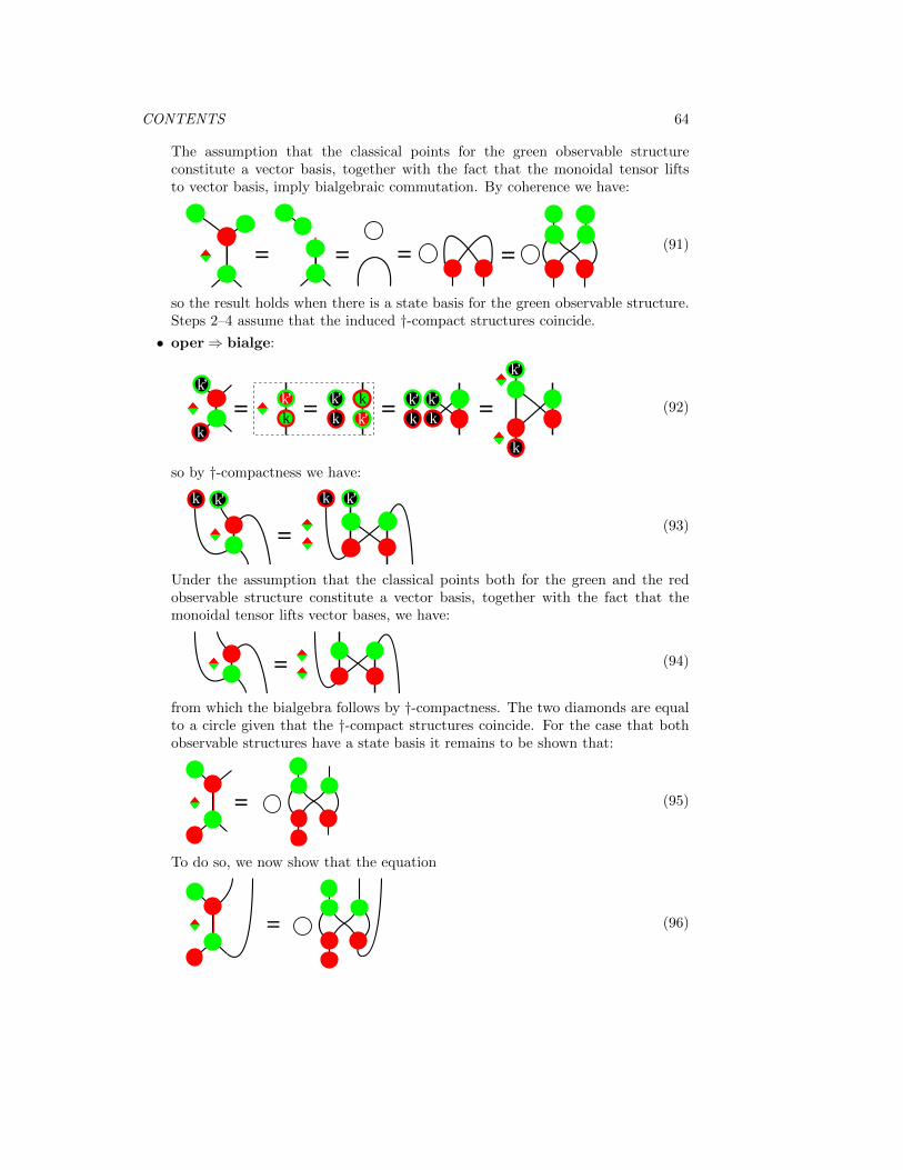
CONTENTS 64

The assumption that the classical points for the green observable structureconstitute a vector basis, together with the fact that the monoidal tensor liftsto vector basis, imply bialgebraic commutation. By coherence we have:

(91)

so the result holds when there is a state basis for the green observable structure.Steps 2–4 assume that the induced †-compact structures coincide.

• oper⇒ bialge:

k

‘

k

‘

kkk

k

‘

k k

kk

k

‘

k

‘ k

‘

k

‘

(92)

so by †-compactness we have:

k k k

‘

k

‘

(93)

Under the assumption that the classical points both for the green and the redobservable structure constitute a vector basis, together with the fact that themonoidal tensor lifts vector bases, we have:

(94)

from which the bialgebra follows by †-compactness. The two diamonds are equalto a circle given that the †-compact structures coincide. For the case that bothobservable structures have a state basis it remains to be shown that:

(95)

To do so, we now show that the equation

(96)

CONTENTS 65

holds, by relying on the fact that we have a state basis for both observablestructures, and as above, by again relying on †-compactness. We have:

k

k

‘k

k

k

‘ kk

‘

k

‘

(97)

where in the dotted area we used derivation (92) above. Finally:

(98)

where the last step assumes that induced †-compact structures coincide.

This concludes this proof. 2

Remark 9.25. We leave it to the reader to see how ‘2B (+ Coh)’ factors intorequirements for oper⇒ comul and comul⇒ bialge.

The examples of cos discussed in Proposition 9.20 satisfy all the equations statedin Theorem 9.24. In particular, they constitute scaled bialgebras. These equations arestrictly stronger than the Hopf law by Theorem 9.15, and hence all pairs of observablestructures that satisfy them are cos.

10. Further group structure and the classical automorphisms

In Section 7.4 we saw how the abelian group of phase shifts arose naturally from thepresence of unbiased points for a given observable structure. When we have a pair ofcos, the two phase groups can interfere with each other, an interaction which arisesfrom the special role of the classical points within each phase group.

In the following, suppose (A, δZ , εZ) and (A, δX , εX) are coherent cos whichjointly form a scaled bialgebra. Let UZ denote all the unbiased points for (δZ , εZ),and let KZ denote its classical points; define UX and KX similarly. By virtue ofcomplementarity we have KX ⊆ UZ and KZ ⊆ UX . Recall that by Proposition 7.19,(UZ ,�Z) is an abelian group, isomorphic to the phase group of (δZ , εZ).

Theorem 10.1. KX is a subgroup of (UZ ,�Z) if either: KX is finite; or, if the twoobservable structures give rise to the same †-compact structure.

Proof. KX is always a submonoid of UZ because of the closure and coherence of thetwo observable structures; any finite submonoid is a subgroup. Alternatively, given apoint x ∈ KX , its inverse in UZ is given by its conjugate with respect to the †-compactstructure of (δZ , εZ); by the definition of classicality, x is self-conjugate with respectto the †-compact structure of (δX , εX). Hence, if these †-compact structures agree (cf.Proposition 8.2), x−1 = x in UZ , so KX is a subgroup. 2

CONTENTS 66

Remark 10.2. Shared †-compact structure is a powerful assumption. The proofabove indicates that in the case of coinciding †-compact structures, not only do theclassical points within UZ form a subgroup, but the resulting group is a product ofcopies of S2. In the case of qubits described by X and Z spins, the †-compact structureis shared, and the resulting classical subgroup is just S2.

Proposition 10.3. For all x ∈ KX , ΛZ(x) is a left action on UZ and, in particular,is a permutation on KX .

Proof. For any ψ : I → A, we have ΛZ(x) ◦ ψ = x �Z ψ by definition; that this is apermutation on KX follows from the closure of KX . 2

Theorem 10.4. Suppose k ∈ KZ , and define K = ΛX(k); then K is a groupautomorphism of UZ .

Proof. Graphically we depict K as:

K =k

k . (99)

Since k ∈ UX , K is unitary, and so is invertible. We must show that if α ∈ UZ thenalso K ◦α ∈ UZ . This holds if and only if ΛZ(K ◦α) is unitary; we show this directly:

ブk

-ブ-k

ブ

-ブ

k

-k

-k

k

ブ -k

-ブ k

-k

k

(100)

where the equations are by the comultiplication property, the unitarity of K, theunbiasedness of α, and the unitarity of K again. It remains to show that K is ahomomorphism of the group structure.

(i) K ◦ (α�Z β) = (K ◦ α)�Z (K ◦ β) :

k

ブ プ

k kk

k k

ブ ブ ブプ プ プ

k

ブ プ. (101)

The equations are: the definition of K; the bialgebra law; the classical propertyof k; and the definition of K.

(ii) K ◦ ε†Z = ε†Z (upto global phase):

k

k

k. (102)

The equation simply uses coherence of δX and εZ ; the result follows by dividingby the scalar factor as per Lemma 7.16.

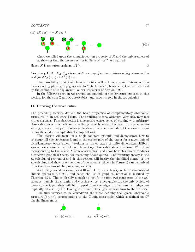
CONTENTS 67

(iii) (K ◦ α)−1 = K ◦ α−1:

ブk

-ブk

ブ

k

-ブ

k

(103)

where we relied upon the comultiplication property of K and the unbiasedness ofα, showing that the inverse K ◦ α in UZ is K ◦ α−1 as required.

Hence K is an automorphism of UZ . 2

Corollary 10.5. (KZ ,�X) is an abelian group of automorphisms on UZ whose actionis defined by (x, z) 7→ ΛX(x) ◦ z.

The possibility that the classical points will act as automorphisms on thecorresponding phase group gives rise to “interference” phenomena; this is illustratedby the example of the quantum Fourier transform of Section 3.2.3.

In the following section we provide an example of the structure exposed in thissection, for the spin Z and X observables, and show its role in the zx-calculus.

11. Deriving the zx-calculus

The preceding sections derived the basic properties of complementary observablestructures in an arbitrary †-smc. The resulting theory, although very rich, may feelrather abstract. This abstraction is a necessary consequence of working with arbitraryobservable structures, without specifying exactly what they are. In any concretesetting, given a fixed pair of observable structures, the remainder of the structure canbe constructed via simple direct computations.

This section will focus on a single concrete example and demonstrate how toconstruct all the structures found in the earlier part of the paper for a given pair ofcomplementary observables. Working in the category of finite dimensional Hilbertspaces, we choose a pair of complementary observable structures over C2—thosecorresponding to the Z and X spin observables—and show how this choice producesa concrete graphical theory for reasoning about qubits. The resulting theory is thezx-calculus of sections 2 and 3: this section will justify the simplified syntax of thezx-calculus, and show that the rules of the calculus (shown in Figure 1) can be derivedfrom the theorems of the preceding sections.

As already noted in examples 4.10 and 4.19, the category of finite dimensionalHilbert spaces is a †-smc, and hence the use of graphical notation is justified byTheorem 4.24. This is already enough to justify the first two generators of the zx-calculus, namely the straight and crossing wires. Since qubits are the only system ofinterest, the type labels will be dropped from the edges of diagrams: all edges areimplicitly labelled by C2. Having introduced the edges, we now turn to the vertices.

The first vertices to be considered are those defining the ‘green’ observablestructure (δZ , εZ), corresponding to the Z-spin observable, which is defined on C2

via the linear maps,

δZ : |i〉 7→ |ii〉 εZ :√

2 |+〉 7→ 1

CONTENTS 68

As discussed in Example 7.22, the points which are unbiased for (δZ , εZ) have theform |αZ〉 = |0〉 + eiα |1〉 where 0 ≤ α < 2π, and hence the phase group consists ofmatrices of the form:

ΛZ(|αZ〉) =

(1 00 eiα

)= α .

The group (UZ ,�Z) is therefore isomorphic to the circle, and the operation �Z isaddition modulo 2π. The Pauli-Z matrix is given by ΛZ(π). Notice also that

ブ =

α

† =

(1 00 eiα

)†=

(1 00 e−iα

)= -ブ

hence we can drop the “corners” from the diagrammatic notation and simply writethe negative angle in its place.

α 7→ ブ ブ 7→ -ブ

The spider rules (Theorem 7.11) justify the first part of the zx-calculus syntax, thefamily of ‘green’ vertices Zmn (α), along with rule (S1) and the first part of rule (S2).

The X-observable structure is essentially the same: defining (δX , εX) as follows:

δX : |±〉 7→ |±±〉 εX :√

2 |0〉 7→ 1

and it is easy to verify that the corresponding phase group consists of rotations aroundX, that is, matrices of the form

ΛX(|αX〉) =

(cos α2 i sin α

2i sin α

2 cos α2

)= α ,

generated by the (unnormalised) unbiased points |αX〉 =√

2(cos α2 |0〉 + i sin α2 |1〉).

We can simplify the notation as we did for the Z-observable:

α 7→ ブ ブ 7→ -ブ

Of course, the decorated spider rules also apply to (δX , εX), and this produces the‘red’ family of the zx-calculus, the vertices Xm

n (α).To complete rule (S2), we appeal to one property not derived from the formalism

of complementary observables, namely the fact that (δZ , εZ) and (δX , εX) induce thesame compact structure:

= δZ ◦ ε†Z

= δX ◦ ε†X

= |00〉+ |11〉 =

CONTENTS 69

Hence we obtain the remaining part of rule (S2), as well as the bending wires.Further, since each object now comes with a unique †-compact structure, we can

treat the category as †-compact, and appeal to Theorem 4.26. This justifies rule (T),“only the topology matters”.

Having noted that (δZ , εZ) and (δX , εX) generate the same †-compact structure,we may also appeal to Lemma 9.4, that is:

= = = .

Now, setting = (D1), Proposition 9.5 produces rule (D2) of the zx-calculus.The definition of δZ immediately shows that the classical points of the Z

observable are |0〉 and |1〉; these points are unbiased for (δX , εX), corresponding tothe angles 0 and π in (UX ,�X). Similarly, the classical points of δX are |+〉 and |−〉,which are unbiased for (δZ , εZ), and again correspond to the angles 0 and π. Thisbeing the case, we can again simplify the graphical notation, and dispense with thetwo-coloured dots used in sections 8 and 9 in favour of a simpler convention:

a dot is unbiased for the observable structure of the same colour;

if it is labelled by π or zero then it is classical for the other structure. In the zx-calculusthere is no need for dots of any other kind, so we disallow them. The translationbetween the more general graphical language and the simplfied version used in thezx-calculus is summarised in table 1.

General: α α k k k k

Simplified:ブ ブ π π Not Allowed

Table 1. Translation between general and simplified graphical notation

Since each structure’s classical points are unbiased for the other structure,(δZ , εZ) and (δX , εX) are complementary as per definition 8.1. Furthermore, we have

ε†X =√

2 |0〉 and ε†Z =√

2 |+〉, so the two observable structures are also coherent as indefinition 9.1, implying rule (B1) of the zx-calculus.

The classical points of Z correspond to the angles 0 and π within the phase groupof X, and vice versa. Since these angles form a two-element subgroup within thecircle group, (δX , εX) and (δZ , εZ) form a closed pair of complementary observablesstructures, as per definition 9.17. Noting that the triple {|0〉 , |1〉 , |+〉} forms a statebasis for C2, the conditions for Theorem 9.24 are satisfied: from whence, bialgebraiccommutation (definition 9.11) implies rule (B2), and comultiplicative commutation(definition 9.9) implies rule (K1).

The remaining piece of the structure to be described is the action of KZ on UZdiscussed in Section 10. Since X1

1 (π) = X we see that the non-trivial element of KZsends |αZ〉 7→ |−αZ〉; i.e. X assigns elements of UZ to their inverses. The action ofKX on UX is exactly dual. This provides the rule (K2) of the zx-calculus. The groupstructure is summarised in Table 2.

The preceding has shown that the zx-calculus, with one exception, is readilydeduced from the algebraic properties of the Z and X observables: indeed everything

CONTENTS 70

Observable Classical Points Unbiased Points Phase Group

Z = (δZ , εZ) |0〉 , |1〉 |0〉+ eiα |1〉 Zα =

(1 00 eiα

), , π

α α

X = (δX , εX) |+〉 , |−〉 cos α2 |0〉+ i sin α2 |1〉 Xα =

(cos α2 i sin α

2i sin α

2 cos α2

), , π

α α

Observable Classical Subgroup Automorphism Action

Z = (δZ , εZ) 1,X X : Zα 7→ Z−α

, , ππ

α

−α=

X = (δX , εX) 1,Z Z : Xα 7→ X−α

, , ππ

α

−α=

Table 2. Summary of the group structure for qubits

else followed from that choice. The single exception is the H vertex and the associatedrule (C). The addition of a special symbol for the Hadamard gate is simply to makecertain calculations easier, and it is not essential to the calculus.

12. Non-determinism, mixed states, and classical data flow

The graphical treatment so far has been limited to pure states, and therefore does notcapture the full behavour of quantum measurements, decoherence, classical control,and a host of other phenomena of great practical importance in quantum computation.

This section will present three different extensions of the graphical lanaguage toaccount for mixed states, and dispense with the simplified treatment of measurementsas projections. We briefly describe each of these, and provide the same example ineach one: the quantum teleportation protocol. For full details, see the references.

The most general is Selinger’s CPM construction [68] which, given any categoryof “pure states” and “pure maps”, constructs a category of “mixed states” and“completely positive maps”. Within the resulting category, Paquette, Pavlovic and oneof the authors defined a plethora of classicality-related concepts such as decoherence,

CONTENTS 71

measurement, probability distribution, stochastic map, function on classical data, etc.,by relying on observable structure [25] —some of these results were already presentin Carboni and Walters’ seminal paper [12]. An axiomatic account on Selinger’sCPM construction and classical concepts therein was provided by Perdrix and anauthor of this paper [16, 29]; this introduces a new element to the graphical calculuscorresponding to the environment, and a corresponding axiom (and some ‘coherenceconditions’). Finally, Perdrix and the other author of this paper have introduceda version of the zx-calculus parameterised by a set of variables which encode theoutcome of measurements, and the dependence of other elements upon them. Theseconditional diagrams have been used in the context of measurement-based quantumcomputation to study determinism and information flow [37].

These three approaches are alternatives, and depending on the situation one maybe preferable to another.

12.1. The CPM construction and classical concepts therein [68, 25]

We extend the graphical language by a construction which is formally similar to theway in which classical probabilities are described by density operators. Graphically,classical data and classical operations are represented by a single wire, while quantumdata and quantum operations are represented by double wires. The passage from adouble wire to a single via a dot encodes decoherence. This encoding:

1 wire/box

classical=

2 wires/boxes

quantum

is also present in Dirac notation; for a mixed state∑i ωi|ψi〉〈ψi| the clasical

probabilistic state (ω1, . . . , ωn) occurs only once while the quantum states occur bothas a ket |ψi〉 and as a bra 〈ψi|. Pure quantum operations, controlled pure quantumoperations, and destructive measurements are of the forms:

f f

f ff f ,

respectively, where for clarity we choose to colour the classical wires in the colour ofthe observable structure whose classical points will encode the classical data.

In fact, the spiders of the graphical language were initially introduced underthe name classical structures in [27] to model classical data in quantum informaticprotocols. Hence, in this setting, a single concept can account both for quantumobservables, complementarity, phases, as well as classical information flow. We willbe very brief on the use of spiders in order to describe classical data flow; we refer thereader to [25] for more details.

Example 12.1. We claim that the following constitutes the quantum teleportationprotocol, including the classical correction:

CONTENTS 72

Bell state

(1) = Alice’s Bell basis measurement

(2) =Bob’s Pauli corrections

(1)

(2)

.

The green and the red wire represent the two qubits Alice has to send to Bob to informhim of the measurement outcome. The Bell state, Bob’s Pauli corrections and Alice’sBell basis measurement can be rewritten respectively as:

.

hence, they are of the forms shown above.The picture might seem somewhat complicated; the reason for this is that in order

to display the quantum-classical distinction graphically, all the quantum operationsare doubled. If we hide one of the copies it becomes much clearer what is going on:

.

We demonstrate that the measurement and corrections in this picture are indeedthe ones we claim them to be. By ‘selecting’ the control operation, that is, by inserting

CONTENTS 73

a classical point at the input, we obtain the Pauli corrections:

k

‘

k

kk

‘

=

= I

ππ = Z

π π = X

ππ

= X ◦ Z

Similarly, by post-‘selecting’ the measurement outcome, that is, by inserting theadjoint of a classical point at the output, we obtain the Bell-basis measurement:

k

‘

k

k

‘

k =

= |00〉+ |11〉

Zπ π = |00〉 − |11〉

π π = |01〉+ |10〉

π π = |01〉 − |10〉

We now compute the overall result of the teleportation protocol diagrammatically:

= = = ... =T2S B’ B’S

Note how the B′-rule causes the flow of classical data to disconnect from the flow ofquantum data, which of course, should not depend on classical data anymore. Thescalars that remain at the end are a consequence of the fact that we didn’t normalisethe Bell state, nor the Bell basis measurement, nor the B′-rule; if we had done so allscalars would have cancelled out.

12.2. Classicality via environment [16, 29]

Roughly equivalent to the above ‘construction’ is the following ‘axiomatic account’—see [16] for the precise correspondence. We consider two kinds of morphisms, ‘pureones’ (or ‘sharp’) and ‘mixed ones’ (or ‘unsharp’). We represent the pure morphismsas we did throughout this paper:

B

Af

CONTENTS 74

and the mixed ones, for example, as rounded variants of the pure ones:

B

A

f

We then introduces a new graphical element , one for each object, which is

coherent with the †-compact structure, and is subject to an axiom:

A

Aff

Agg

A

iffAf

Ag (104)

which is valid for all pure morphisms f : A→ B and g : A→ C. To obtain a precisematch with the CPM construction, we also need a purification axiom which statesthat any mixed morphism can be obtained from a pure one by composing the latterwith the environment. From (104) it follows that classical channels, that is:

or

are idempotent [29]. Here the color reflects how the classical data was obtained, i.e.,in which measurement. This idempotence in fact the only equation which plays somerole in the teleportation protocol, which now goes as follows:

12.3. Conditional diagrams [37]

While the previous two approaches represent classical information flow internally, asparticular wires in the diagrams, the final alternative presentation of non-determinismignores the issue of (classical) information flow, and focuses on classical correlationswhich are mediated externally.

Let V be a set of formal variables. A conditional diagram is a diagram D of the zx-calculus and, for each Z and X vertex v in D, an associated subset Uv ⊆ V, possiblyempty. A valuation is function f : V → {0, 1}. Each pair (D, f) of a conditionaldiagram and a valuation determines an evaluated diagram Df , which is obtained fromD by modifying the phase α at each vertex v as follows:

α 7→{α if

∏u∈Uv f(u) = 1

0 otherwise

and forgetting the sets Uv. Each variable corresponds to a two-valued measurementand each valuation f corresponds to a possible set of measurement outcomes.The evaluated diagram Df corresponds to the process that occurs when themeasurement outcomes corresponding f are observed, including both the side-effect

CONTENTS 75

of the measurement itself, and any other operations which depend classically upon itsoutcome.

Since each Df is a diagram of the zx-calculus, it has an associated linear map,Df , as described in Section 2.3. We construct a superoperator for D by summing overall possible valuations:

D : ρ 7→∑f

DfρD†f .

Conditional diagrams can use the same equational rules as the plain zx-calculus, withthe proviso that a rule can only be applied in D if it could be applied to every Df .

The conditional diagrams approach is essentially a formalisation of the informalreasoning demonstrated in Section 3.3.1, as the following example wil clearlydemonstrate.

Example 12.2. Let V = {a, b}, where each variable corresponds to one of thesingle-qubit measurements comprising the Bell basis measurement in the teleportationprotocol. Teleportation protocol can then be formalised as follows:

in

out

Bob

H

π π

Alice

ππ{a}{a}

{b}{b}

=

ππ{a}

{b}

ππ {a}{b}

=

π{a}

π {a}

The crux of the encoding is that the subdiagram

M = π {a}denotes the superoperator

ρ 7→ 〈+| ρ |+〉+ 〈−| ρ |−〉 ,and thus correctly encodes the measurement.

The conditional diagram approach is very well suited to the one-way model,since the quantum part of the system can be very complicated, whereas the classicalinformation flow can ususally be taken for granted. For many purposes, for exampleto translate a one-way pattern to a circuit, we need not evaluate any valuation, andcan simply use the equational rules on the conditional diagram directly.

The measurement calculus [30] includes several commands which depend uponon classical bits, here ranged over by s and t:

• s[Mαj ]t – measure qubit j in the basis |0〉+ e(−1)

si(α+tπ) |1〉.• Xs

j and Zsj – apply a Pauli X operator (or Z) to qubit j, if s = 1; otherwise donothing.

Taking V to be the set of measured qubits in the pattern, the measurement calculuscan be encoded using conditional diagrams according to the table below.

Ni Eij Mαi Xi

s Zit

Hπ {i} π {i} π {i}

CONTENTS 76

Note that conditional measurement s[Mαi ]t is equivalent to the sequence Mα

i Xsi Z

ti ,

and therefore can be replaced by it.

Example 12.3. Consider the pattern:

Xv34 Zv24 Zv21 M0

3M02E13E23E34N3N4.

An unreliable quantum software engineer claims that it computes the a ∧X on itsinputs, regardless of the result of the measurements. We can check this claim usingequational reasoning on the conditional diagram. Let V = {v2, v3}, corresponding tothe outcomes of the measument of qubits 2 and 3.

H

π

H

H

π π

π

{v2} {v

2}{v

3}

{v3}

=H

πH

H

π

π

π{v2}

{v2}

{v3}

{v3}

=H

πH

H

π

π{v2}

{v2}

{v3}

{v3}

π=

H

πH

H

{v2}

{v2}π

=H

π H

H

{v2}

{v2}

π{v

2}π =

H

πH

H

π{v2} {v

2}

π{v2} =

π {v2}

Since the final diagram still has the variable v2 occuring in it, the original claim wasfalse: the result of this pattern depends upon the result of the measurement. Howeverfrom the diagram we can can easily debug the pattern by adding a final correctionZv24 correction at the end. The corrected pattern is:

Zv24 Xv34 Zv21 M0

3M02E13E23E34N3N4.

These ideas are developed more fully in [37].

Remark 12.4. The notion of conditional diagrams, and their superoperatorinterpretation, can be easily generalised beyond the minimal setting we have presentedhere. Variables could take values in an arbitrary set A—indeed not all variablesneed have the same set of values—and the modification of the diagram based on thevaluation function could be arbitarily more complicated without changing anythingessential. Finally, given an interpretation functor from diagrams into some †-symmetric monoidal category C, then a “superoperator” can be constructed usinga suitable semigroup enrichment of C.

13. Conclusion

In this paper we introduced a simple and intuitive— but at the same time universal—graphical calculus for qubits, the zx-calculus, and gave many example applications.We studied its mathematical underpinning in great detail, in particular:

CONTENTS 77

• We obtained a purely diagrammatic characterization of complementarity thatextends to observable structures in arbitrary †-smcs, in terms of the Hopf law:

• We identified a strong form of complementarity for observable structures inarbitrary †-smcs, when the observable structures form a scaled bialgebra:

.

We identified a number of equivalent alternative formulations:

kk k

kkk

k

‘

k

‘

k

‘

k k,k k, k k,

• We identified a group structure on phases for observable structures in arbitrary†-smcs, and proved a generalization of the spider rules, now involving phases:

.

As already mentioned at the end of the introduction, meanwhile our results havebeen applied in many contexts, ranging from quantum information and quantumfoundations to automated reasoning.

We end by mentioning a number of issues that require further exploration:

• Is there an elegant extension of the zx-calculus to a zxy-calculus? Note that thiswill necessarily involve the dualisers of Section 8.2. Would such a zxy-calculusbe different when either modeling Stab or Spek? (cf. Example 7.23)

• What is the precise connection between the stabiliser formalism and ourgraphical reasoning scheme? (Given that both are adequate tools for studyingmeasurement-based quantum computing.) Is the stabiliser formalism andquantum error correction fully captured by the zx-calculus?

• Theorem 10.1 adds extra structure with a clear physical interpretation to thephase group: while the elements of K may be seen as measurement outcomes, thecorresponding cosets can be interpreted as choices of measurements. This mayprovide a foundation for an axiomatic analysis of non-locality and contextuality.Some work in this direction has already been done [39].

• Can the zx-calculus elegantly model many body states other than graph states,e.g., matrix product states or other states arising in condensed matter physics?

• Does our characterization of complementarity extend in some way or anotherto observables described by infinite dimensional Hilbert spaces? What is theconnection of the above depicted laws to canonical commutation relations?

CONTENTS 78

Acknowledgements

Work supported by the authors’ respective epsrc advanced and postdoctoral researchfellowships, by the fnrs, by ec fp6 strep qics, by an fqxi large grant and by onrgrant, and we also acknowledge support of Perimeter Institute for Theoretical Physicswhich hosted both of the authors. We thank Bertfried Fauser, Prakash Panangaden,Simon Perdrix, Stefano Pironio, Marni Dee Sheppeard and the referees for valuablefeedback on an earlier version of this paper, and to Stephen Brierly and Stefan Weigertfor providing the counter-example of Remark 9.22.

14. References

[1] S. Abramsky and B. Coecke (2004) A categorical semantics of quantum protocols. Proceedings ofthe 19th Annual IEEE Symposium on Logic in Computer Science (LiCS‘04), IEEE ComputerSociety Press. arXiv:quant-ph/0402130

[2] S. Abramsky and B. Coecke (2005) Abstract physical traces. Theory and Applications ofCategories 14, 111–124. www.tac.mta.ca/tac/volumes/14/6/14-06abs.html

[3] S. Abramsky and N. Tzevelekos (2011) Introduction to categories and categorical logic. In: NewStructures for Physics, B. Coecke, Ed. Springer lecture Notes in Physics, vol 813, p3–94.

[4] L. Amico, R. Fazio, A. Osterloh and V. Vedral (2008) Entanglement in many-body systems.Reviews of Modern Physics 80, 517–576. arXiv:quant-ph/0703044

[5] F. Baader and T. Nipkow (1999) Term Rewriting and All That. Cambridge University Press.[6] J. Baez and M. Stay (2011) Physics, topology, logic and computation: a Rosetta Stone. In: New

Structures for Physics, B. Coecke, Ed. Springer lecture Notes in Physics, vol 813, p95–172.[7] J. Barrett (2007) Information processing in general probabilistic theories. Physical Review A

75, 032304. arXiv:quant-ph/0508211[8] C. H. Bennett, G. Brassard, C. Crepeau, R. Jozsa, A. Peres and W. K. Wooters (1993)

Teleporting an unknown quantum state via dual classical and Einstein-Podolsky-Rosenchannels. Physical Review Letters 70, 1895–1899.

[9] G. Birkhoff (1958) von Neumann and lattice theory. Bulletin of the American MathematicalSociety 64, 50–56.

[10] G. Birkhoff (1961) Lattices in Applied Mathematics. In R. P. Dilworth (ed.) Lattice Theory,Proceedings of the Second Symposium in Pure Mathematics of the American MathematicalSociety, April 1959, Providence: American Mathematical Society

[11] G. Birkhoff and J. von Neumann (1936) The logic of quantum mechanics. Annals of Mathematics37, 823–843.

[12] A. Carboni and R. F. C. Walters (1987) Cartesian bicategories I. Journal of Pure and AppliedAlgebra 49, 11–32.

[13] P. Cartier (2006) A primer of Hopf algebras. IHES preprint.[14] B. Coecke (2006) Introducing categories to the practicing physicist. In: What is Category

Theory? pages 45–74. Advanced Studies in Mathematics and Logic 30, PolimetricaPublishing. arXiv:0808.1032

[15] B. Coecke (2007) De-linearizing linearity: projective quantum axiomatics from strong compactclosure. Electronic Notes in Theoretical Computer Science 170, 49–72. arXiv:quant-ph/

0506134

[16] B. Coecke (2008) Axiomatic description of mixed states from Selinger’s CPM-construction.Electronic Notes in Theoretical Computer Science 210, 3–13.

[17] B. Coecke (2010) Quantum picturalism. Contemporary Physics 51, 59–83. arXiv:0908.1787[18] B. Coecke and R. Duncan (2008) Interacting quantum observables. In L. Aceto, I. Damgard,

L. A. Goldberg, M. M. Halldorsson, A Ingolfsdottir, and I. Walukiewic, editors, Automata,Languages and Programming, 35th International Colloquium, ICALP 2008, Reykjavik,Iceland, July 7-11, 2008, Proceedings, Part II, volume 5126 of Lecture Notes in ComputerScience, pages 298–310. Springer, 2008.

[19] B. Coecke and B. Edwards (2011) Toy quantum categories. In: Proceedings of QuantumPhysics and Logic/Development of Computational Models (QPL-DCM). Electronic Notesin Theoretical Computer Science, vol 271 (1), pp 29–40. arXiv:0808.1037

[20] B. Coecke, B. Edwards and R. W. Spekkens (2011) Phase groups and the origin of non-locality for qubits. Electronic Notes in Theoretical Computer Science, vol 271 (2), pp 15–36.arXiv:1003.5005

CONTENTS 79

[21] B. Coecke and A. Kissinger (2010) The Compositional Structure of Multipartite QuantumEntanglement. In Automata, Languages and Programming, 37th International Colloquium,ICALP 2010, Proceedings Part II, volume 6199 of Lecture Notes in Computer Science, pages297–308. Springer. arXiv:1002.2540.

[22] B. Coecke, D. J. Moore and A. Wilce (2000) Operational quantum logic: An overview. In:Current Research in Operational Quantum Logic: Algebras, Categories and Languages,B. Coecke, D. J. Moore and A. Wilce (eds), pages 1–36. Fundamental Theories of Physics111, Springer-Verlag. arXiv:quant-ph/0008019

[23] B. Coecke and E. O. Paquette (2006) POVMs and Naimark’s theorem without sums. ElectronicNotes in Theoretical Computer Science, vol 210, pp 131–152. arXiv:quant-ph/0608072

[24] B. Coecke and E. O. Paquette (2011) Categories for the practicing physicist. In: New Structuresfor Physics, B. Coecke, Ed., Springer lecture Notes in Physics, vol 813, pp 173–286.arXiv:0905.3010

[25] B. Coecke, E. O. Paquette and D. Pavlovic (2009) Classical and quantum structuralism. InSemantic Techniques for Quantum Computation, I. Mackie and S. Gay (eds), pp 29–26Cambridge University Press. arXiv:0904.1997

[26] B. Coecke, E. O. Paquette and S. Perdrix (2008) Bases in diagrammatic quantum protocols.Electronic Notes in Theoretical Computer Science, vol 218, pp 131–152. arXiv:0808.1037

[27] B. Coecke and D. Pavlovic (2007) Quantum measurements without sums. In: Mathematics ofQuantum Computing and Technology, G. Chen, L. Kauffman and S. Lomonaco (eds), pages567–604. Taylor and Francis. arXiv:quant-ph/0608035

[28] B. Coecke, D. Pavlovic, and J. Vicary (2008) A new description of orthogonal bases.Mathematical Structures in Computer Science, to appear. arXiv:0810.0812

[29] B. Coecke and S. Perdrix (2010) Environment and classical channels in categorical quantummechanics. In: Proceedings of the 19th EACSL Annual Conference on Computer ScienceLogic (CSL), Lecture Notes in Computer Science 6247, pp 230–244, Springer-Verlag.arXiv:1004.1598

[30] V. Danos, E. Kashefi and P. Panangaden (2007) The measurement calculus. Journal of the ACM54 (2). arXiv:quant-ph/0412135

[31] D. G. B. J. Dieks (1982) Communication by EPR devices. Physics Letters A 92, 271–272.[32] L. Dixon, R. Duncan and A. Kissinger. Quantomatic. http://dream.inf.ed.ac.uk/projects/

quantomatic/

[33] L. Dixon and R. Duncan (2009) Graphical reasoning in compact closed categories for quantumcomputation. Annals of Mathematics and Artificial Intelligence, 56, 23–42.

[34] L. Dixon and A. Kissinger (2010) Open graphs and monoidal theories. arXiv:1011.4114[35] R. Duncan (2006) Types for Quantum Computing. D.Phil. thesis. Oxford University.[36] R. Duncan and S. Perdrix (2009) Graph states and the necessity of Euler decomposition.

In Computability in Europe: Mathematical Theory and Computational Practice (CiE’09),volume 5635 of Lecture Notes in Computer Science, pages 167–177. Springer.arXiv:0902.0500

[37] R. Duncan and S. Perdrix (2010) Rewriting measurement-based quantum computations withgeneralised flow. In Automata, Languages and Programming, 37th International Colloquium,ICALP 2010, Proceedings Part II, volume 6199 of Lecture Notes in Computer Science, pages285–296. Springer.

[38] W. Dur, G. Vidal and J. I. Cirac (2000) Three qubits can be entangled in two inequivalent ways.Physical Review A 62, 062314.

[39] B. Edwards (2010) Phase groups and local hidden variables. Oxford University Comput-ing Laboratory Research Report RR-10-15. http://www.comlab.ox.ac.uk/publications/

publication3716-abstract.html

[40] H. Ehrig, K. Ehrig, U. Prange, and G. Taentzer (2006) Fundamentals of Algebraic GraphTransformation. Monographs in Theoretical Computer Science. Springer.

[41] J. Evans, R. Duncan, A. Lang, and p. Panangaden (2009) Classifying all mutually unbiasedbases in rel. arxiv:0909.4453

[42] P. Freyd and D. Yetter (1989) Braided compact closed categories with applications to low-dimensional topology. Advances in Mathematics 77, 156–182.

[43] C. A. Fuchs (2001) Quantum foundations in the light of quantum information. In: Decoherenceand its Implications in Quantum Computation and Information Transfer: Proceedings ofthe NATO Advanced Research Workshop, Mykonos Greece, June 25-30, 2000, pages 38–82,A.‘Gonis and P. E. A. Turchi, eds. IOS Press. arXiv:quant-ph/0106166

[44] R. Haag (1992) Local Quantum Physics: Fields, Particles, Algebras. Springer-Verlag.[45] L. Hardy (2001) Quantum theory from five reasonable axioms. arXiv:quant-ph/0101012

CONTENTS 80

[46] J. M. Jauch (1968) Foundations of Quantum Mechanics. Addison-Wesley.[47] A. Joyal and R. Street (1991) The Geometry of tensor calculus I. Advances in Mathematics 88,

55–112.[48] A. Joyal and R. Street (1993) Braided Tensor Categories. Advances in Mathematics 102, 20–78.[49] R. Jozsa (2006) An introduction to measurement based quantum computation. In Dimitris G.

Angelakis, Matthias Christiandl, Artur Ekert, Alastair Kay, and Sergei Kulik, editors,Quantum information processing: from theory to experiment, pages 137–158. IOS Press.

[50] C. Kassel (1995) Quantum groups. Graduate Texts in Mathematics 155, Springer-Verlag.[51] G. M. Kelly and M. L. Laplaza (1980) Coherence for compact closed categories. Journal of Pure

and Applied Algebra 19, 193–213.[52] G.M. Kelly and S. Mac Lane (1971) Coherence in closed categories. Journal of Pure and

Applied Algebra 1, 97–140.[53] J. Kock (2003) Frobenius Algebras and 2D Topological Quantum Field Theories. Cambridge UP.[54] S. Lack (2004) Composing PROPs. Theory and Applications of Categories 13, 147–163.[55] G. Ludwig (1985) An Axiomatic Basis of Quantum Mechanics. 1. Derivation of Hilbert Space.

Springer-Verlag.[56] G. Ludwig (1987) An Axiomatic Basis of Quantum Mechanics. 2. Quantum Mechanics and

Macrosystems. Springer-Verlag.[57] S. Mac Lane (1998) Categories for the Working Mathematician. 2nd edition. Springer-Verlag.[58] N. D. Mermin (1990) Quantum mysteries revisited. American Journal of Physics 58, 731–734.[59] M. Nielsen and I. Chuang (2000) Quantum Computation and Quantum Information. Cambridge

University Press.[60] D. Pavlovic (2009) Quantum and classical structures in nondeterminstic computation. Lecture

Notes in Computer Science 5494, page 143–157, Springer. arXiv:0812.2266[61] R. Penrose (1971) Applications of negative dimensional tensors. In: Combinatorial Mathematics

and its Applications, pages 221–244. Academic Press.[62] S. Perdrix (2005) State transfer instead of teleportation in measurement-based quantum

computation. International Journal of Quantum Information 3, 219–223. arXiv:quant-ph/0402204

[63] I. Pitowski (1989) Quantum Probability, Quantum Logic. Springer-Verlag, Heidelberg.[64] R. Raussendorf and H. J. Briegel (2001) A one-way quantum computer. Phys. Rev. Lett., 86,

5188–5191.[65] R. Raussendorf, D. Browne and H. J. Briegel (2003) Measurement-based quantum computation

on cluster states. Physical Review A 68, 022312. arXiv:quant-ph/0301052[66] M. Redei (1997) Why John von Neumann did not like the Hilbert space formalism of quantum

mechanics (and what he liked instead). Studies in History and Philosophy of Modern Physics27, 493–510.

[67] E. Schrodinger (1935) Discussion of probability relations between separated systems. Proceedingsof the Cambridge Philosophical Society 31, 555–563.

[68] P. Selinger (2005) Dagger compact closed categories and completely positive maps. ElectronicNotes in Theoretical Computer Science 170, 139–163. www.mathstat.dal.ca/∼selinger/papers.html]dagger

[69] P. Selinger (2011) A survey of graphical languages for monoidal categories. In: New Structuresfor Physics, B. Coecke, Ed. Springer lecture Notes in Physics, vol 813, pp289-355.

[70] P. Selinger (2010) Autonomous categories in which A ' A∗. Extended abstract. In: Proceedingsof the 7th International Workshop on Quantum Physics and Logic, May 29-30, Oxford.www.mscs.dal.ca/∼selinger/papers.html]halftwist

[71] P. W. Shor (1997) Polynomial-time algorithms for prime factorization and discrete logarithmson a quantum computer. SIAM Journal on Computing 26, 1484–1509.

[72] R. Spekkens (2007) Evidence for the epistemic view of quantum states: A toy theory. PhysicalReview A 75, 032110.

[73] R. Street (2007) Quantum Groups: A Path to Current Algebra. Cambridge University Press.[74] W. Tadej and K. Zyczkowski (2006) A concise guide to complex Hadamard matrices. Open

Systems & Information Dynamics 13 (2).[75] M. Van den Nest, J. Dehaene, and B. De Moor (2004) Graphical description of the action of

local clifford transformations on graph states. Physical Review A 69, 022316.[76] F. Verstraete and J. I. Cirac (2004) Valence-bond states for quantum computation. Physical

Review A 70, 060302(R). arXiv:quant-ph/0311130[77] W. K. Wootters and W. Zurek (1982) A single quantum cannot be cloned. Nature 299, 802–803.