Inter-iteration Scalar ReplacementUsing Array SSA Form

Rishi Surendran1, Rajkishore Barik2, Jisheng Zhao1, and Vivek Sarkar1

1 Rice University, Houston, TX{rishi,jisheng.zhao,vsarkar}@rice.edu

2 Intel Labs, Santa Clara, CArajkishore.barik@intel.com

Abstract. In this paper, we introduce novel simple and efficient analy-sis algorithms for scalar replacement and dead store elimination that arebuilt on Array SSA form, a uniform representation for capturing controland data flow properties at the level of array or pointer accesses. Wepresent extensions to the original Array SSA form representation to cap-ture loop-carried data flow information for arrays and pointers. A corecontribution of our algorithm is a subscript analysis that propagates ar-ray indices across loop iterations. Compared to past work, this algorithmcan handle control flow within and across loop iterations and degradegracefully in the presence of unanalyzable subscripts. We also introducecode transformations that can use the output of our analysis algorithmsto perform the necessary scalar replacement transformations (includingthe insertion of loop prologues and epilogues for loop-carried reuse). Ourexperimental results show performance improvements of up to 2.29× rel-ative to code generated by LLVM at -O3 level. These results promise tomake our algorithms a desirable starting point for scalar replacementimplementations in modern SSA-based compiler infrastructures such asLLVM.

Keywords: Static Single Assignment (SSA) form, Array SSA form, Scalar Re-placement, Load Elimination, Store Elimination

1 Introduction

Scalar replacement is a widely used compiler optimization that promotes mem-ory accesses, such as a read of an array element or a load of a pointer location, toreads and writes of compiler-generated temporaries. Current and future trendsin computer architecture provide an increased motivation for scalar replacementbecause compiler-generated temporaries can be allocated in faster and moreenergy-efficient storage structures such as registers, local memories and scratch-pads. However, scalar replacement algorithms in past work [6, 9, 7, 3, 14, 4, 2, 21,5] were built on non-SSA based program representations, and tend to be com-plex to understand and implement, expensive in compile-time resources, andlimited in effectiveness in the absence of precise data dependences. Though thebenefits of SSA-based analysis are well known and manifest in modern compilerinfrastructures such as LLVM [13], it is challenging to use SSA form for scalar

replacement analysis since SSA form typically focuses on scalar variables andscalar replacement focuses on array and pointer accesses.

In this paper, we introduce novel simple and efficient analysis algorithmsfor scalar replacement and dead store elimination that are built on Array SSAform [12], an extension to scalar SSA form that captures control and data flowproperties at the level of array or pointer accesses. We present extensions tothe original Array SSA form representation to capture loop-carried data flowinformation for arrays and pointers. A core contribution of our algorithm is asubscript analysis that propagates array indices across loop iterations. Comparedto past work, this algorithm can handle control flow within and across loop it-erations and degrades gracefully in the presence of unanalyzable subscript. Wealso introduce code transformations that can use the output of our analysis algo-rithms to perform the necessary scalar replacement transformations (includingthe insertion of loop prologs and epilogues for loop-carried reuse). These resultspromise to make our algorithms a desirable starting point for scalar replacementimplementations in modern SSA-based compiler infrastructures.

The main contributions of this paper are:

• Extensions to Array SSA form to capture inter-iteration data flow informa-tion of arrays and pointers

• A framework for inter-iteration subscript analysis for both forward and back-ward data flow problems

• An algorithm for inter-iteration redundant load elimination analysis usingour extended Array SSA form, with accompanying transformations for scalarreplacement, loop prologs and loop epilogues.

• An algorithm for dead store elimination using our extended Array SSA form,with accompanying transformations.

The rest of the paper is organized as follows. Section 2 discusses backgroundand motivation for this work. Section 3 contains an overview of scalar replace-ment algorithms. Section 4 introduces Array SSA form and extensions for inter-iteration data flow analysis. Section 5 presents available subscript analysis, aninter-iteration data flow analysis. Section 6 describes the code transformationalgorithm for redundant load elimination, and Section 7 describes the analysisand transformations for dead store elimination. Section 8 briefly summarizeshow our algorithm can be applied to objects and while loops. Section 9 containsdetails on the LLVM implementation and experimental results. Finally, Section10 presents related work and Section 11 contains our conclusions.

2 Background

In this section we summarize selected past work on scalar replacement whichfalls into two categories. 1) inter-iteration scalar replacement using non-SSArepresentations and 2) intra-iteration scalar replacement using Array SSA form,to provide the background for our algorithms. A more extensive comparison withrelated work is presented later in Section 10.

(a) Original Loop (b) After Scalar Replacement1: for i = 1 to n do2: B[i] = 0.3333 ∗ (A[i− 1] +A[i] +A[i+ 1])3: end for

1: t0 = A[0]2: t1 = A[1]3: for i = 1 to n do4: t2 = A[i+ 1]5: B[i] = 0.3333 ∗ (t0 + t1 + t2)6: t0 = t17: t1 = t28: end for

Fig. 1. Scalar replacement on a 1-D Jacobi stencil computation [1]

2.1 Inter-iteration Scalar Replacement

Figure 1(a) shows the innermost loop of a 1-D Jacobi stencil computation [1].The number of memory accesses per iteration in the loop is four, which includesthree loads and a store. The read references involving array A present a reuseopportunity in that the data read by A[i + 1] is also read by A[i] in the nextiteration of the loop. The same element is also read in the following iterationby A[i − 1]. The reference A[i + 1] is referred to as the generator [7] for theredundant loads, A[i] and A[i − 1]. The number of memory accesses inside theloop could thus be reduced to one, if the data read by A[i+1] is stored in a scalartemporary which could be allocated to faster memory. Assuming n > 0, the loopafter scalar replacement transformation is shown in 1(b). Non-SSA algorithms forinter-iteration scalar replacement have been presented in past work including [6,7, 9]. Of these, the work by Carr and Kennedy [7] is described below, since it isthe most general among past algorithms for inter-iteration scalar replacement.

2.2 Carr-Kennedy Algorithm

The different steps in the Carr-Kennedy algorithm [7] are 1) Dependence graphconstruction, 2) Control flow analysis, 3) Availability analysis, 4) Reachabilityanalysis, 5) Potential generator selection, 6) Anticipability analysis, 7) Depen-dence graph marking, 8) Name partitioning, 9) Register pressure moderation, 10)Reference replacement, 11) Statement insertion analysis, 12) Register copying,13) Code motion, and 14) Initialization of temporary variables.

The algorithm is complex, requires perfect dependence information to beapplicable and operates only on loop bodies without any backward conditionalflow. Further, the algorithm performs its profitability analysis on name parti-tions, where a name partition consists of references that share values. If a namepartition is selected for scalar replacement, all the memory references in thatname partition will get scalar replaced, otherwise none of the accesses in thename partition are scalar replaced.

2.3 Array SSA Analysis

Array SSA is a program representation which captures precise element-leveldata-flow information for array variables. Every use and definition in the ex-

tended Array SSA form has a unique name. There are 3 different types of φfunctions presented in [10].

1. A control φ (denoted simply as φ) corresponds to the φ function from scalarSSA. A φ function is added for a variable at a join point if multiple definitionsof the variable reach that point.

2. A definition φ (dφ) [12] is used to deal with partially killing definitions. Adφ function of the form Ak = dφ(Ai, Aj) is inserted immediately after eachdefinition of the array variable, Ai, that does not completely kill the arrayvalue. Aj is the augmenting definition of A which reaches the point justprior to the definition of Ai. A dφ function merges the value of the elementmodified with the values that are available prior to the definition.

3. A use φ (uφ) [10] function creates a new name whenever a statement reads anarray element. The purpose of the uφ function is to link together uses of thesame array in control-flow order. This is used to capture the read-after-readreuse (aka input dependence). A uφ function of the form Ak = uφ(Ai, Aj)is inserted immediately after the use of an array element, Ai. Aj is theaugmenting definition of A which reaches the point just prior to the use ofAi.

[10] presented a unified approach for the analysis and optimization of objectfield and array element accesses in strongly typed languages using Array SSAform. But the approach had a major limitation in that it does not capturereuse across loop iterations. For instance, their approach cannot eliminate theredundant memory accesses in the loop in Figure 1. In Section 4, we introduceextensions to Array SSA form for inter-iteration analysis.

2.4 Definitely-Same and Definitely-Different Analyses

In order to reason about aliasing among array accesses, [10] describes two rela-tions: DS represents the Definitely-Same binary relationship and DD representsthe Definitely-Different binary relationship. DS(a, b) = true if and only if a andb are guaranteed to have the same value at all program points that are dom-inated by the definition of a and dominated by the definition of b. Similarly,DD(a, b) = true if and only if a and b are guaranteed to have different valuesat all program points that are dominated by the definition of a and dominatedby the definition of b. The Definitely-same (DS) and Definitely-different (DD)relation between two array subscripts can be computed using different methodsand is orthogonal to the analysis and transformation described in this paper.

3 Scalar Replacement Overview

In this section, we present an overview of the basic steps of our scalar replacementalgorithms: redundant load elimination and dead store elimination. To simplifythe description of the algorithms, we consider only a single loop. We also assumethat the induction variable of the loop has been normalized to an incrementof one. Extensions to multiple nested loops can be performed in hierarchical

fashion, starting with the innermost loop and analyzing a single loop at a time.When analyzing an outer loop, the array references in the enclosed nested loopsare summarized with subscript information [16].

The scalar replacement algorithms include three main steps:

1. Extended Array SSA Construction:In the first step, the extended Array SSA form of the original program isconstructed. All array references are renamed and φ functions are introducedas described in Section 4. Note that the extended Array SSA form of the pro-gram is used only for the analysis (presented in step 2). The transformations(presented in step 3) are applied on the original program.

2. Subscript analysis:Scalar replacement of array references is based on two subscript analyses: (a)available subscript analysis identifies the set of redundant loads in the givenloop, which is used for redundant load elimination (described in Section 6);(b) dead subscript analysis identifies the set of dead stores in the given loop,which is used in dead store elimination (described in Section 7). These anal-yses are performed on extended Array SSA form and have an associatedtuning parameter: the maximum number of iterations for which the analysisneeds to run.

3. Transformation:In this step, the original program is transformed using the information pro-duced by the analyses described in step 2. For redundant load elimination,this involves replacing the read of array elements with read of scalar tem-poraries, generating copy statements for scalar temporaries and generatingstatements to initialize the temporaries. The transformation is presented inSection 6. Dead store elimination involves removing redundant stores andgenerating epilogue code as presented in Section 7.

4 Extended Array SSA Form

1: for i = 1 to n do2: if A[B[i]] > 0 then3: A[i+1] = A[i-1] + B[i-1]4: end if5: A[i] = A[i] + B[i] + B[i+1]6: end for

Fig. 2. Loop with redundant loads and stores

In order to model inter-iteration reuse, the latticeoperations of the φ functionin the loop header needsto be handled differentlyfrom the rest of the con-trol φ functions. They needto capture what array el-ements are available fromprior iterations. We introduce a header φ (hφ) node in the loop header. Weassume that every loop has one incoming edge from outside and thus, one of thearguments to the hφ denotes the SSA name from outside the loop. For each backedge from within the loop, there is a corresponding SSA operand added to the hφfunction. Figure 2 shows a loop from [11, p. 387] extended with control flow. Thethree address code of the same program is given in 3(a) and the extended ArraySSA form is given in 3(b). A1 = hφ(A0, A12) and B1 = hφ(B0, B10) are the two

hφ nodes introduced in the loop header. A0 and B0 contain the definitions ofarray A which reaches the loop preheader.

While constructing Array SSA form, dφ and uφ functions are introduced firstinto the program. The control φ and hφ functions are added in the second phase.This will ensure that the new SSA names created due to the insertion of uφ anddφ nodes are handled correctly. We introduce at most one dφ function for eacharray definition and at most one uφ function for each array use. Past work haveshown that the worst-case size of the extended Array SSA form is proportionalto the size of the scalar SSA form that would be obtained if each array access ismodeled as a definition [10]. Past empirical results have shown the size of scalarSSA form to be linearly proportional to the size of the input program [8].

(a) Three Address Code (b) Array SSA form

1: for i = 1 to n do2: t1 = B[i]3: t2 = A[t1]4: if t2 > 0 then5: t3 = A[i− 1]6: t4 = B[i− 1]7: t5 = t3 + t48: A[i+ 1] = t59: end if

10: t6 = A[i]11: t7 = B[i]12: t8 = B[i+ 1]13: t9 = t6 + t714: t10 = t9 + t815: A[i] = t1016: end for

1: A0 = ...2: B0 = ...3: for i = 1 to n do4: A1 = hφ(A0, A12)5: B1 = hφ(B0, B10)6: t1 = B2[i]7: B3 = uφ(B2, B1)8: t2 = A2[t1]9: A3 = uφ(A2, A1)

10: if t2 > 0 then11: t3 = A4[i− 1]12: A5 = uφ(A4, A3)13: t4 = B4[i− 1]14: B5 = uφ(B4, B3)15: t5 = t3 + t416: A6[i+ 1] = t5

17: A7 = dφ(A6, A5)18: end if19: A8 = φ(A3, A7)20: B6 = φ(B3, B5)21: t6 = A9[i]22: A10 = uφ(A9, A8)23: t7 = B7[i]24: B8 = uφ(B7, B6)25: t8 = B9[i+ 1]26: B10 = uφ(B9, B8)27: t9 = t6 + t728: t10 = t9 + t829: A11[i] = t1030: A12 = dφ(A11, A10)31: end for

Fig. 3. Example Loop and extended Array SSA form

5 Available Subscript Analysis

In this section, we present the subscript analysis which is one of the key ingre-dients for inter-iteration redundant load elimination (Section 6) and dead storeelimination transformation (Section 7). The subscript analysis takes as input theextended Array SSA form of the program and a parameter, τ , which representsthe maximum number of iterations across which inter-iteration scalar replace-ment will be applied on. An upper bound on τ can be obtained by computing themaximum dependence distance for the given loop, when considering all depen-dences in the loop. However, since smaller values of τ may sometimes be betterdue to register pressure moderation reasons, our algorithm views τ as a tuningparameter. This paper focuses on the program analysis foundations of our scalarreplacement approach — it can be combined with any optimization strategy formaking a judicious choice for τ .

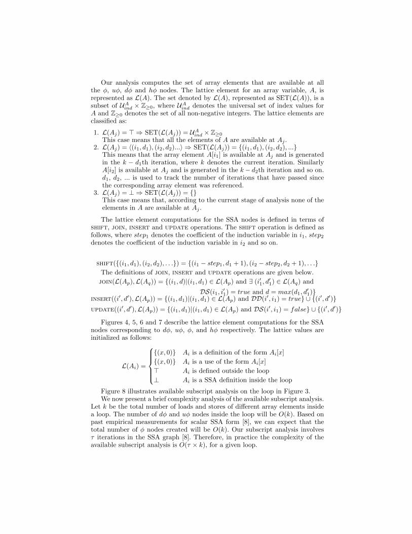
Our analysis computes the set of array elements that are available at allthe φ, uφ, dφ and hφ nodes. The lattice element for an array variable, A, isrepresented as L(A). The set denoted by L(A), represented as SET(L(A)), is asubset of UA

ind × Z≥0, where UAind denotes the universal set of index values for

A and Z≥0 denotes the set of all non-negative integers. The lattice elements areclassified as:

1. L(Aj) = > ⇒ SET(L(Aj)) = UAind × Z≥0

This case means that all the elements of A are available at Aj .2. L(Aj) = 〈(i1, d1), (i2, d2)...〉 ⇒ SET(L(Aj)) = {(i1, d1), (i2, d2), ...}

This means that the array element A[i1] is available at Aj and is generatedin the k − d1th iteration, where k denotes the current iteration. SimilarlyA[i2] is available at Aj and is generated in the k− d2th iteration and so on.d1, d2, ... is used to track the number of iterations that have passed sincethe corresponding array element was referenced.

3. L(Aj) = ⊥ ⇒ SET(L(Aj)) = {}This case means that, according to the current stage of analysis none of theelements in A are available at Aj .

The lattice element computations for the SSA nodes is defined in terms ofshift, join, insert and update operations. The shift operation is defined asfollows, where step1 denotes the coefficient of the induction variable in i1, step2denotes the coefficient of the induction variable in i2 and so on.

shift({(i1, d1), (i2, d2), . . .}) = {(i1 − step1, d1 + 1), (i2 − step2, d2 + 1), . . .}The definitions of join, insert and update operations are given below.

join(L(Ap),L(Aq)) = {(i1, d)|(i1, d1) ∈ L(Ap) and ∃ (i′1, d′1) ∈ L(Aq) and

DS(i1, i′1) = true and d = max(d1, d

′1)}

insert((i′, d′),L(Ap)) = {(i1, d1)|(i1, d1) ∈ L(Ap) and DD(i′, i1) = true} ∪ {(i′, d′)}update((i′, d′),L(Ap)) = {(i1, d1)|(i1, d1) ∈ L(Ap) and DS(i′, i1) = false} ∪ {(i′, d′)}

Figures 4, 5, 6 and 7 describe the lattice element computations for the SSAnodes corresponding to dφ, uφ, φ, and hφ respectively. The lattice values areinitialized as follows:

L(Ai) =

{(x, 0)} Ai is a definition of the form Ai[x]

{(x, 0)} Ai is a use of the form Ai[x]

> Ai is defined outside the loop

⊥ Ai is a SSA definition inside the loop

Figure 8 illustrates available subscript analysis on the loop in Figure 3.We now present a brief complexity analysis of the available subscript analysis.

Let k be the total number of loads and stores of different array elements insidea loop. The number of dφ and uφ nodes inside the loop will be O(k). Based onpast empirical measurements for scalar SSA form [8], we can expect that thetotal number of φ nodes created will be O(k). Our subscript analysis involvesτ iterations in the SSA graph [8]. Therefore, in practice the complexity of theavailable subscript analysis is O(τ × k), for a given loop.

L(Ar) L(Ap) = > L(Ap) = 〈(i1, d1), . . .〉 L(Ap) = ⊥L(Aq) = > > > >L(Aq) = 〈(i′, d′)〉 > insert((i′, d′), 〈(i1, d1), . . .〉) 〈(i′, d′)〉L(Aq) = ⊥ ⊥ ⊥ ⊥

Fig. 4. Lattice computation for L(Ar) = Ldφ(L(Aq),L(Ap)) where Ar := dφ(Aq, Ap)is a definition φ operation

L(Ar) L(Ap) = > L(Ap) = 〈(i1, d1), . . .〉 L(Ap) = ⊥L(Aq) = > > > >L(Aq) = 〈(i′, d′)〉 > update((i′, d′), 〈(i1, d1), . . .〉) L(A1)L(Aq) = ⊥ > L(Ap) ⊥

Fig. 5. Lattice computation for L(Ar) = Luφ(L(Aq),L(Ap)) where Ar := uφ(Aq, Ap)is a use φ operation

L(Ar) = L(Aq) u L(Ap) L(Ap) = > L(Ap) = 〈(i1, d1), . . .〉 L(Ap) = ⊥L(Aq) = > > L(Ap) ⊥L(Aq) = 〈(i′1, d′1), . . .〉 L(Aq) join(L(Aq),L(Ap)) ⊥L(Aq) = ⊥ ⊥ ⊥ ⊥

Fig. 6. Lattice computation for L(Ar) = Lφ(L(Aq),L(Ap)), where Ar := φ(Aq, Ap) isa control φ operation

L(Ar) L(Ap) = > L(Ap) = 〈(i1, d1), . . .〉 L(Ap) = ⊥L(Aq) = > > L(Ap) ⊥L(Aq) = 〈(i′1, d′1), . . .〉 shift(L(Aq)) join(shift(L(Aq)),L(Ap)) ⊥L(Aq) = ⊥ ⊥ ⊥ ⊥

Fig. 7. Lattice computation for L(Ar) = Lhφ(L(Aq),L(Ap)), where Ar := hφ(Aq, Ap)is a header φ operation

Iteration 1 Iteration 2

L(A1) ⊥ {(i− 1, 1)}L(B1) ⊥ {(i− 1, 1), (i, 1)}L(B3) {(i, 0)} {(i− 1, 1), (i, 0)}L(A3) {(t, 0)} {(i− 1, 1), (t, 0)}L(A5) {(i− 1, 0), (t, 0)} {(i− 1, 0), (t, 0)}L(B5) {(i− 1, 0), (i, 0)} {(i− 1, 0), (i, 0)}L(A7) {(i− 1, 0), (i+ 1, 0)} {(i− 1, 0), (i+ 1, 0)}L(A8) ⊥ {(i− 1, 1)}L(B6) {(i, 0)} {(i− 1, 1), (i, 0)}L(A10) {(i, 0)} {(i− 1, 1), (i, 0)}L(B8) {(i, 0)} {(i− 1, 1), (i, 0)}L(B10) {(i, 0), (i+ 1, 0)} {(i− 1, 1), (i, 0), (i+ 1, 0)}L(A12) {(i, 0)} {(i− 1, 1), (i, 0)}

Fig. 8. Available Subscript Analysis Example

6 Load Elimination Transformation

In this section, we present the algorithm for redundant load elimination. Thereare two steps in the algorithm: Register pressure moderation described in Sec-tion 6.1, which determines a subset of the redundant loads for load eliminationand Code generation described in Section 6.2, which eliminates the redundantloads from the loop.

The set of redundant loads in a loop is represented using UseRepSet, a setof ordered pairs of the form (Aj [x], d), where the use Aj [x] is redundant and dis the iteration distance from the generator to the use. d = 0 implies an intra-iteration reuse and d ≥ 1 implies an inter-iteration reuse. UseRepSet is derivedfrom the lattice sets computed by available subscript analysis.

UseRepSet = { (Ai[x], d) | ∃ (y, d) ∈ L(Aj), Ak = uφ(Ai, Aj), DS(x, y) = true}

For the loop in Figure 3, UseRepSet = {(B2[i], 1), (A4[i−1], 1), (B4[i−1], 1), (B7[i], 0)}

6.1 Register Pressure Moderation

Eliminating all redundant loads in a loop may lead to generation of spill codewhich could counteract the savings from scalar replacement. To prevent this, weneed to choose the most profitable loads which could be scalar replaced usingthe available machine registers. We define the most profitable loads as the oneswhich requires the least number of registers.

When estimating the total register requirements for scalar replacement, allredundant uses which are generated by the same reference need to be consideredtogether. To do this UseRepSet is partitioned into U1, ...Uk, such that generatorsof all uses in a partition are definitely-same. A partition represents a set of useswhich do not dominate each other and are generated by the same use/def. Apartition Um is defined as follows, where step is the coefficient of the inductionvariable in the subscript expression.

Um = {(Ai[xi], di) | ∀ (Aj [xj ], dj) ∈ Um,DS(xi + di × step, xj + dj × step) =true}

If the array index expression is loop-invariant, the number of registers re-quired for its scalar replacement is one. In other cases, the number of registersrequired for eliminating all the loads in the partition Up is given by

NumRegs(Up) = {di + 1 | (Ai[xi], di) ∈ Up ∧ ∀ (Aj [xj ], dj) ∈ Up, di ≥ dj}For the loop in Figure 3, the four elements in UseRepSet will fall into four

different partitions: {(B2[i], 1)}, {(A4[i−1], 1)}, {(B4[i−1], 1)}, {(B7[i], 0)}. Thetotal number of registers required for the scalar replacement is 7.

The partitions are then sorted in increasing order of the number of registersrequired. To select the redundant loads for scalar replacement, we use a greedyalgorithm in which at each step the algorithm chooses the first available partition.The algorithm terminates when the first available partition does not fit into theremaining machine registers.

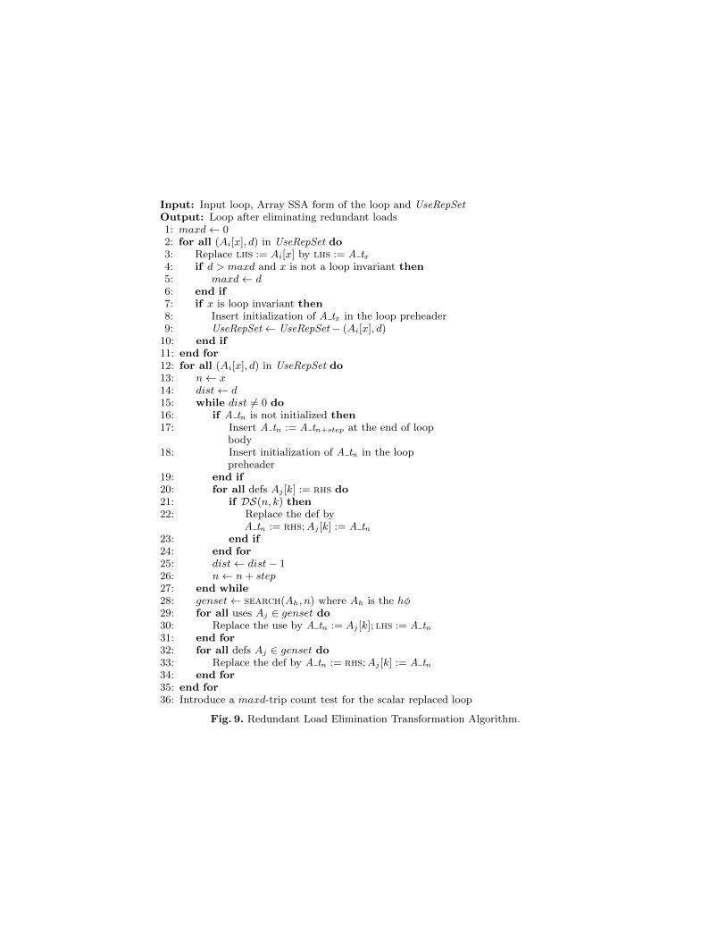
Input: Input loop, Array SSA form of the loop and UseRepSetOutput: Loop after eliminating redundant loads1: maxd← 02: for all (Ai[x], d) in UseRepSet do3: Replace lhs := Ai[x] by lhs := A tx4: if d > maxd and x is not a loop invariant then5: maxd← d6: end if7: if x is loop invariant then8: Insert initialization of A tx in the loop preheader9: UseRepSet← UseRepSet− (Ai[x], d)

10: end if11: end for12: for all (Ai[x], d) in UseRepSet do13: n← x14: dist← d15: while dist 6= 0 do16: if A tn is not initialized then17: Insert A tn := A tn+step at the end of loop

body18: Insert initialization of A tn in the loop

preheader19: end if20: for all defs Aj [k] := rhs do21: if DS(n, k) then22: Replace the def by

A tn := rhs;Aj [k] := A tn23: end if24: end for25: dist← dist− 126: n← n+ step27: end while28: genset← search(Ah, n) where Ah is the hφ29: for all uses Aj ∈ genset do30: Replace the use by A tn := Aj [k]; lhs := A tn31: end for32: for all defs Aj ∈ genset do33: Replace the def by A tn := rhs;Aj [k] := A tn34: end for35: end for36: Introduce a maxd-trip count test for the scalar replaced loop

Fig. 9. Redundant Load Elimination Transformation Algorithm.

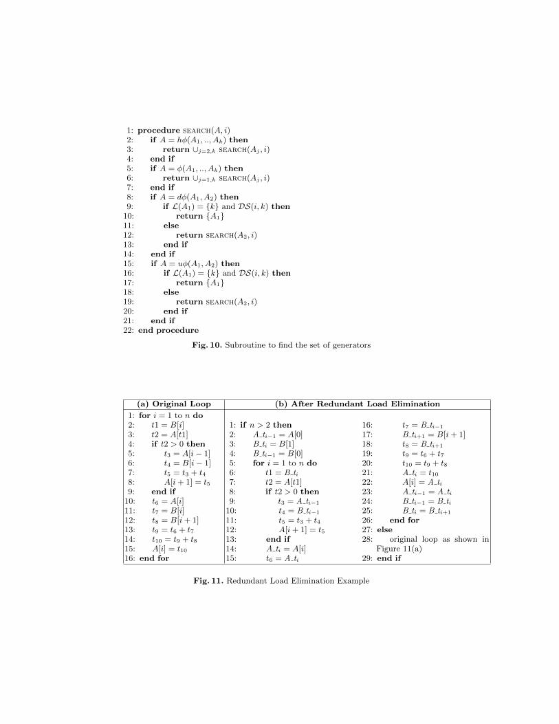
1: procedure search(A, i)2: if A = hφ(A1, .., Ak) then3: return ∪j=2,k search(Aj , i)4: end if5: if A = φ(A1, .., Ak) then6: return ∪j=1,k search(Aj , i)7: end if8: if A = dφ(A1, A2) then9: if L(A1) = {k} and DS(i, k) then

10: return {A1}11: else12: return search(A2, i)13: end if14: end if15: if A = uφ(A1, A2) then16: if L(A1) = {k} and DS(i, k) then17: return {A1}18: else19: return search(A2, i)20: end if21: end if22: end procedure

Fig. 10. Subroutine to find the set of generators

(a) Original Loop (b) After Redundant Load Elimination

1: for i = 1 to n do2: t1 = B[i]3: t2 = A[t1]4: if t2 > 0 then5: t3 = A[i− 1]6: t4 = B[i− 1]7: t5 = t3 + t48: A[i+ 1] = t59: end if

10: t6 = A[i]11: t7 = B[i]12: t8 = B[i+ 1]13: t9 = t6 + t714: t10 = t9 + t815: A[i] = t1016: end for

1: if n > 2 then2: A ti−1 = A[0]3: B ti = B[1]4: B ti−1 = B[0]5: for i = 1 to n do6: t1 = B ti7: t2 = A[t1]8: if t2 > 0 then9: t3 = A ti−1

10: t4 = B ti−1

11: t5 = t3 + t412: A[i+ 1] = t513: end if14: A ti = A[i]15: t6 = A ti

16: t7 = B ti−1

17: B ti+1 = B[i+ 1]18: t8 = B ti+1

19: t9 = t6 + t720: t10 = t9 + t821: A ti = t1022: A[i] = A ti23: A ti−1 = A ti24: B ti−1 = B ti25: B ti = B ti+1

26: end for27: else28: original loop as shown in

Figure 11(a)29: end if

Fig. 11. Redundant Load Elimination Example

6.2 Code Generation

The inputs to the code generation algorithm are the intermediate representationof the loop body, the Array SSA form of the loop, and the subset of UseRepSetafter register pressure moderation. The code transformation is performed on theoriginal input program. The extended Array SSA form is used to search for thegenerator corresponding to a redundant use. The algorithm for the transforma-tion is shown in Figure 9. A scalar temporary, A tx is created for every arrayaccess A[i] that is scalar replaced where, DS(x, i) = true. In the first stage of thealgorithm all redundant loads are replaced with a reference to a scalar temporaryas shown in lines 2-11 of Figure 9. For example the reads of array elements B[i]in line 1, A[i− 1] in line 5, B[i− 1] in line 6 and B[i] in line 11 of Figure 11(a)are replaced with reads of scalar temporaries as shown in Figure 11(b). The loopalso computes the maximum iteration distance for all redundant uses to theirgenerator. It also moves loop invariant array reads to loop preheader. The loopin lines 15-27 of Figure 9 generates copy statements between scalar temporariesand code to initialize scalar temporaries if it is a loop carried reuse. The code toinitialize the scalar temporary is inserted in the loop preheader, the basic blockthat immediately dominates the loop header. Line 2-4 in Figure 11(b) is thecode generated to initialize the scalar temporaries and lines 23-25 are the copystatements generated to carry values across iterations. The loop in lines 20-24of Figure 9 guarantees that the scalar temporaries have the right values if thevalue is generated across multiple iterations. Lines 28-35 of Figure 9 identifiesthe generators and initializes the appropriate scalar temporaries. The generatorsare identified using the recursive search routine SEARCH, which takes two argu-ments: The first argument is a SSA function Aj and the second argument is anindex i. The function returns the set of all uses/defs which generates A[i]. TheSEARCH routine is given in Figure 10. The routine takes at most one backwardtraversal of the SSA graph to find the set of generators. Line 36 of the loadelimination algorithm inserts a loop trip count test around the scalar replacedloop.

We now present a brief complexity analysis of the load elimination transfor-mation described in Figure 9. Let k be the total number of loads and stores ofarray elements inside the loop and let l be the number of redundant loads. Thealgorithm makes l traversals of the SSA graph and examines the stores inside theloop a maximum of l × d, where d is the maximum distance from the generatorto the redundant use. Therefore the worst case complexity of the algorithm inFigure 9 for a given loop is O((d+ 1)× l × k).

7 Dead Store Elimination

Elimination of loads can increase the number of dead stores inside the loop. Forexample, consider the loop in Figure 12(a). The store of A[i+ 1] in line 2 is usedby the load of A[i] in line 3. Assuming n > 0, Figure 12(b) shows the same loopafter scalar replacement and elimination of redundant loads. The store of A[i+1]in line 5 for the first n− 1 iterations is now redundant since it gets overwrittenby the store to A[i] at line 7 in the next iteration with no uses in between.

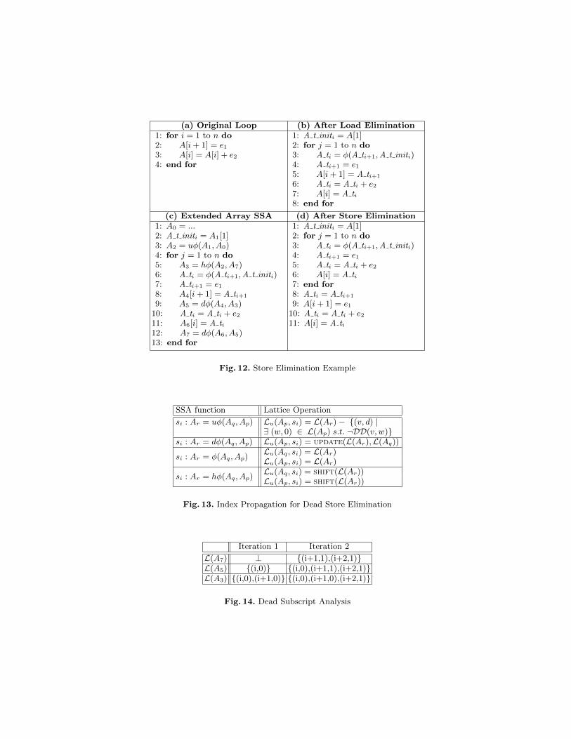
(a) Original Loop (b) After Load Elimination1: for i = 1 to n do2: A[i+ 1] = e13: A[i] = A[i] + e24: end for

1: A t initi = A[1]2: for j = 1 to n do3: A ti = φ(A ti+1,A t initi)4: A ti+1 = e15: A[i+ 1] = A ti+1

6: A ti = A ti + e27: A[i] = A ti8: end for

(c) Extended Array SSA (d) After Store Elimination1: A0 = ...2: A t initi = A1[1]3: A2 = uφ(A1, A0)4: for j = 1 to n do5: A3 = hφ(A2, A7)6: A ti = φ(A ti+1,A t initi)7: A ti+1 = e18: A4[i+ 1] = A ti+1

9: A5 = dφ(A4, A3)10: A ti = A ti + e211: A6[i] = A ti12: A7 = dφ(A6, A5)13: end for

1: A t initi = A[1]2: for j = 1 to n do3: A ti = φ(A ti+1,A t initi)4: A ti+1 = e15: A ti = A ti + e26: A[i] = A ti7: end for8: A ti = A ti+1

9: A[i+ 1] = e110: A ti = A ti + e211: A[i] = A ti

Fig. 12. Store Elimination Example

SSA function Lattice Operation

si : Ar = uφ(Aq, Ap) Lu(Ap, si) = L(Ar)− {(v, d) |∃ (w, 0) ∈ L(Ap) s.t. ¬DD(v, w)}

si : Ar = dφ(Aq, Ap) Lu(Ap, si) = update(L(Ar),L(Aq))

si : Ar = φ(Aq, Ap)Lu(Aq, si) = L(Ar)Lu(Ap, si) = L(Ar)

si : Ar = hφ(Aq, Ap)Lu(Aq, si) = shift(L(Ar))Lu(Ap, si) = shift(L(Ar))

Fig. 13. Index Propagation for Dead Store Elimination

Iteration 1 Iteration 2

L(A7) ⊥ {(i+1,1),(i+2,1)}L(A5) {(i,0)} {(i,0),(i+1,1),(i+2,1)}L(A3) {(i,0),(i+1,0)} {(i,0),(i+1,0),(i+2,1)}

Fig. 14. Dead Subscript Analysis

Dead store elimination is run as a post pass to redundant load eliminationand it uses a backward flow analysis of array subscripts similar to very busyexpression analysis. The analysis computes set L(Ai) for every SSA function inthe program. Similar to available subscript analysis presented in Section 5, thelattice for dead subscript analysis, L(A) is a subset of UA

ind×Z≥0. Note that therecould be multiple uses of the same SSA name. For instance, the SSA name A3

is an argument of the uφ function in line 12 and the φ function in line 19 in theloop given in Figure 3(b). A backward data flow analysis will have to keep trackof lattice values for each of these values. To achieve this, we associate a latticeelement with each of the uses of the SSA variable represented as Lu(Ai, sj),where sj is a statement in the program which uses the SSA variable Ai.

During the backward flow analysis, index sets are propagated from left toright of φ functions. The lattice operations for the propagation of data flowinformation are shown in Figure 13. The computation of L(Ai) from all the aug-mented uses of Ai is given using the following equation.

L(Ai) =⋂

sj is a φ use of Ai

L(Ai, sj)

The lattice values are initialized as follows:

L(Ai) =

{(x, 0)} Ai is a definition of the form Ai[x]

{(x, 0)} Ai is a use of the form Ai[x]

> Ai is defined outside the loop

⊥ Ai is a SSA function defined inside the loop

The shift and update operations are defined as follows, where step1 is thecoefficient of the induction variable in i1, step2 is the coefficient of the inductionvariable in i2 and so on.

shift〈(i1, d1), (i2, d2), . . .〉 = 〈(i1 + step1, d1 + 1), (i2 + step2, d2 + 1), . . .〉

update((i′, d′),L(Ap)) = {(i1, d1)|(i1, d1) ∈ L(Ap) and DS(i′, i1) = false} ∪ {(i′, d′)}

The result of the analysis is used to compute the set of dead stores:

DeadStores = { (Ai[x], d) | ∃ (y, d) ∈ L(Aj) and DS(x, y) = true and Ak = dφ(Ai, Aj)}

i.e., a store, Ai[x] is redundant with respect to subsequent defs if (y, d) ∈ L(Aj)and DS(x, y) = true, where Ak = dφ(Ai, Aj) is the dφ function correspondingto the use Ai[x]. d represents the number of iterations between the dead storeand the killing store.

Figure 12(c) shows the extended Array SSA form of the program in Fig-ure 12(b). Figure 14 illustrates dead subscript analysis on this loop. The set ofdead stores for this loop is DeadStores = {(A4[i+ 1], 1)}.

Given the set DeadStores = {(S1, d1), ...(Sn, dn)}, the algorithm for deadstore elimination involves peeling the last k iterations of the loop, where k = max

i=1..ndi.

The dead stores could be eliminated from the original loop, but they must beretained in the last k peeled iterations. The loop in Figure 12(b) after the elim-ination of dead stores is given in Figure 12(d).

Similar to available subscript analysis, the worst case complexity of dead sub-script analysis for a given loop is O(τ×k). The complexity of the transformationis O(n), where n is the size of the loop body.

8 Extension to Objects and While Loops

In the previous sections, we introduced new scalar replacement analysis andtransformations based on extended Array SSA form that can be used to optimizearray accesses within and across loop iterations in counted loops. Past work hasshown that scalar replacement can also be performed more generally on objectfields in the presence of arbitrary control flow [10]. However, though the pastwork in [10] used Array SSA form, it could not perform scalar replacementacross multiple iterations of a loop. In this section, we briefly illustrate how ourapproach can also perform inter-iteration scalar replacement in programs withwhile-loops containing accesses to object fields.

Figure 15(a) shows a simple example of a while loop in which the read ofobject field p.x can be replaced by a scalar temporary carrying the value fromthe previous iteration. This code assumes that FIRST and LAST refer to thefirst node and last node in a linked list, and the result of scalar replacement isshown in Figure 15(b). A value of τ = 1 suffices to propagate temp from theprevious iteration to the current iteration, provided a prologue is generated thatis guarded by a zero-trip test as shown in Figure 15(b). It is worth noting that noshape analysis is necessary for the scalar replacement performed in Figure 15(b).If available, shape analysis [20] can be used as a pre-pass to further refine theDS and DD information for objects in while loops.

(a) Original Loop (b) After Scalar Replacement1: p := FIRST2: while p 6= LAST do3: ... = p.x;4: ...5: p = p.next;6: p.x = ...7: end while

1: p := FIRST2: if p 6= LAST then3: temp = p.x;4: end if5: while p 6= LAST do6: ... = temp;7: ...8: p = p.next;9: temp = ...

10: p.x = temp;11: end while

Fig. 15. Scalar replacement example for object accesses in a while loop

9 Experimental Results

In this section, we describe the implementation of our Array SSA based scalarreplacement framework followed by an experimental evaluation of our scalarreplacement and dead store analysis algorithms.

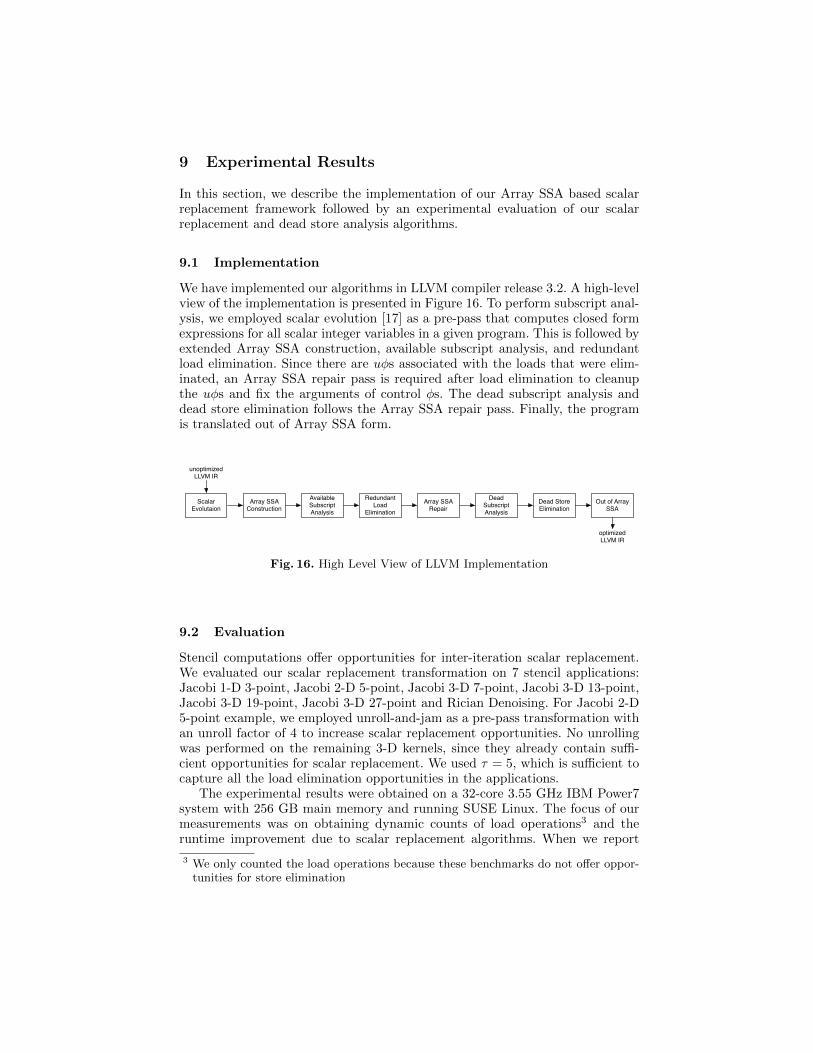
9.1 Implementation

We have implemented our algorithms in LLVM compiler release 3.2. A high-levelview of the implementation is presented in Figure 16. To perform subscript anal-ysis, we employed scalar evolution [17] as a pre-pass that computes closed formexpressions for all scalar integer variables in a given program. This is followed byextended Array SSA construction, available subscript analysis, and redundantload elimination. Since there are uφs associated with the loads that were elim-inated, an Array SSA repair pass is required after load elimination to cleanupthe uφs and fix the arguments of control φs. The dead subscript analysis anddead store elimination follows the Array SSA repair pass. Finally, the programis translated out of Array SSA form.

unoptimizedLLVM IR

Scalar Evolutaion

Array SSA Construction

Available Subscript Analysis

Redundant Load

EliminationArray SSA

RepairDead

Subscript Analysis

Dead Store Elimination

Out of Array SSA

optimizedLLVM IR

Fig. 16. High Level View of LLVM Implementation

9.2 Evaluation

Stencil computations offer opportunities for inter-iteration scalar replacement.We evaluated our scalar replacement transformation on 7 stencil applications:Jacobi 1-D 3-point, Jacobi 2-D 5-point, Jacobi 3-D 7-point, Jacobi 3-D 13-point,Jacobi 3-D 19-point, Jacobi 3-D 27-point and Rician Denoising. For Jacobi 2-D5-point example, we employed unroll-and-jam as a pre-pass transformation withan unroll factor of 4 to increase scalar replacement opportunities. No unrollingwas performed on the remaining 3-D kernels, since they already contain suffi-cient opportunities for scalar replacement. We used τ = 5, which is sufficient tocapture all the load elimination opportunities in the applications.

The experimental results were obtained on a 32-core 3.55 GHz IBM Power7system with 256 GB main memory and running SUSE Linux. The focus of ourmeasurements was on obtaining dynamic counts of load operations3 and theruntime improvement due to scalar replacement algorithms. When we report

3 We only counted the load operations because these benchmarks do not offer oppor-tunities for store elimination

timing information, we report the best wall-clock time from five runs. We usedthe PAPI [15] interface to find the dynamic counts of load instructions executedfor each of the programs. We compiled the programs with two different set ofoptions described below.

– O3 : LLVM -O3 with basic alias analysis.– O3SR : LLVM -O3 with basic alias analysis and scalar replacement

Benchmark O3 Loads O3SR Loads O3 Time (secs) O3SR Time (secs)

Jacobi 1-D 3-Point 5.58E+8 4.59E+8 .25 .25Jacobi 2-D 5-Point 4.35E+8 4.15E+8 .43 .32Jacobi 3-D 7-Point 1.41E+9 1.29E+9 1.66 .74Jacobi 3-D 13-Point 1.89E+9 1.77E+9 2.73 1.32Jacobi 3-D 19-Point 2.39E+9 1.78E+9 3.95 1.72Jacobi 3-D 27-Point 2.88E+9 1.79E+9 5.45 3.16Rician Denoising 2.71E+9 2.46E+9 4.17 3.53

Table 1. Comparison of Load Instructions Executed and Runtimes

Table 1 shows the dynamic counts of load instructions executed and theexecution time for the programs without scalar replacement and with scalarreplacement. All the programs show a reduction in the number of loads whenscalar replacement is enabled. Figure 17 shows the speedup for each of the bench-marks due to scalar replacement. All the programs, except Jacobi 1-D 3-Pointdisplayed speedup due to scalar replacement. The speedup due to scalar replace-ment ranges from 1.18× to 2.29× for different benchmarks.

Fig. 17. Speedup : O3SR with respect to O3

10 Related Work

Region Array SSA [19] is an extension of Array SSA form with explicit ag-gregated array region information for array accesses. Each array definition issummarized using a region representing the elements that it modifies across allsurrounding loop nests. This region information then forms an integral part ofnormal φ operands. A region is represented using an uniform set of references(USR) representation. Additionally, the region is augmented with predicates tohandle control flow. This representation is shown to be effective for constantpropagation and array privatization, but the aggregated region representation ismore complex than the subscript analysis presented in Section 5 and does nothave enough maximum distance information to help guide scalar replacement tomeet a certain register pressure. More importantly, since the region Array SSArepresentation explicitly does not capture use information, it would be hard toperform scalar replacement across iterations for array loads without any inter-vening array store.

A large body of past work has focused on scalar replacement [11, 6, 7, 3, 14]in the context of optimizing array references in scientific programs for betterregister reuse. These algorithms are primarily based on complex data dependenceanalysis and for loops with restricted or no control flow (e.g., [7] only handlesloops with forward conditional control flow). Conditional control flow is oftenignored when testing for data dependencies in parallelizing compilers. Moreover,[7] won’t be able to promote values if dependence distances are not consistent.More recent algorithms such as [3, 14] use analyses based on partial redundancyelimination along with dependence analysis to perform load reuse analysis. Bodiket al. [4] used PRE along with global value-numbering and symbolic informationto capture memory load equivalences.

For strongly typed programming languages, Fink, Knobe and Sarkar [10]presented a unified framework to analyze memory load operations for botharray-element and object-field references. Their algorithm detects fully redun-dant memory operations using an extended Array SSA form representation forarray-element memory operations and global value numbering technique to dis-ambiguate the similarity of object references. Praun et al. [18] presented a PREbased inter-procedural load elimination algorithm that takes into account Java’sconcurrency features and exceptions. All of these approaches do not performinter-iteration scalar replacement.

[5] employed runtime checking that ensures a value is available for stridedmemory accesses using arrays and pointers. Their approach is applicable acrossloop iterations, and also motivated the specialized hardware features such asrotating registers, valid bits, and predicated registers in modern processors.

[21] extend the original scalar replacement algorithm of [7] to outer loopsand show better precision. Extensions for multiple induction variables for scalarreplacement are proposed in [2].

[9] presents a data flow analysis framework for array references which prop-agates iteration distance (aka dependence distance) across loop iterations. Thatis, instances of subscripted references are propagated throughout the loop frompoints where they are generated until points are encountered that kill the in-stances. This information is then applied to optimizations such as redundant load

elimination. Compared to their work, our available subscript analysis operateson SSA form representation and propagates indices instead of just distances.

11 Conclusions

In this paper, we introduced novel simple and efficient analysis algorithms forscalar replacement and dead store elimination that are built on Array SSA form,an extension to scalar SSA form that captures control and data flow propertiesat the level of array or pointer accesses. A core contribution of our algorithm is asubscript analysis that propagates array indices across loop iterations. Comparedto past work, this algorithm can handle control flow within and across loop it-erations and degrades gracefully in the presence of unanalyzable subscripts. Wealso introduced code transformations that can use the output of our analysisalgorithms to perform the necessary scalar replacement transformations (includ-ing the insertion of loop prologues and epilogues for loop-carried reuse). Ourexperimental results show performance improvements of up to 2.29× relative tocode generated by LLVM at -O3 level. These results promise to make our analy-sis algorithms a desirable starting point for scalar replacement implementationsin modern SSA-based compiler infrastructures such as LLVM, compared to themore complex algorithms in past work based on non-SSA program representa-tions.

References

1. Polybench: Polyhedral benchmark suite. http://www.cse.ohio-state.edu/

~pouchet/software/polybench/.2. Nastaran Baradaran, Pedro C. Diniz, and Joonseok Park. Extending the applica-

bility of scalar replacement to multiple induction variables. In Proceedings of the17th international conference on Languages and Compilers for High PerformanceComputing, LCPC’04, pages 455–469, Berlin, Heidelberg, 2005. Springer-Verlag.

3. R. Bodik and R. Gupta. Array Data-Flow Analysis for Load-Store Optimizationsin Superscalar Architectures. Lecture Notes in Computer Science, (1033):1–15, Au-gust 1995. Proceedings of Eighth Annual Workshop on Languages and Compilersfor Parallel Computing, Columbus, Ohio.

4. Rastislav Bodık, Rajiv Gupta, and Mary Lou Soffa. Load-reuse analysis: designand evaluation. SIGPLAN Not., 34(5):64–76, 1999.

5. Mihai Budiu and Seth Copen Goldstein. Inter-iteration scalar replacement in thepresence of conditional control flow. In 3rd Workshop on Optimizations for DSOand Embedded Systems, San Jose, CA, March 2005.

6. David Callahan, Steve Carr, and Ken Kennedy. Improving Register Allocation forSubscripted Variables. Proceedings of the ACM SIGPLAN ’90 Conference on Pro-gramming Language Design and Implementation, White Plains, New York, pages53–65, June 1990.

7. Steve Carr and Ken Kennedy. Scalar Replacement in the Presence of ConditionalControl Flow. Software—Practice and Experience, (1):51–77, January 1994.

8. Ron Cytron, Jeanne Ferrante, Barry K. Rosen, Mark N. Wegman, and F. Ken-neth Zadeck. Efficiently computing static single assignment form and the controldependence graph. ACM Trans. Program. Lang. Syst., 13(4):451–490, October1991.

9. Evelyn Duesterwald, Rajiv Gupta, and Mary Lou Soffa. A practical data flowframework for array reference analysis and its use in optimizations. In Proceed-ings of the ACM SIGPLAN 1993 conference on Programming language design andimplementation, PLDI ’93, pages 68–77, New York, NY, USA, 1993. ACM.

10. Stephen J. Fink, Kathleen Knobe, and Vivek Sarkar. Unified analysis of array andobject references in strongly typed languages. In Proceedings of the 7th Interna-tional Symposium on Static Analysis, SAS ’00, pages 155–174, London, UK, UK,2000. Springer-Verlag.

11. Ken Kennedy and John R. Allen. Optimizing compilers for modern architectures:a dependence-based approach. Morgan Kaufmann Publishers Inc., San Francisco,CA, USA, 2002.

12. Kathleen Knobe and Vivek Sarkar. Array SSA form and its use in Paralleliza-tion. In 25th Annual ACM SIGACT-SIGPLAN Symposium on the Principles ofProgramming Languages, January 1998.

13. Chris Lattner and Vikram Adve. LLVM: A Compilation Framework for LifelongProgram Analysis & Transformation. In Proceedings of the 2004 InternationalSymposium on Code Generation and Optimization (CGO’04), Palo Alto, Califor-nia, Mar 2004.

14. Raymond Lo, Fred Chow, Robert Kennedy, Shin-Ming Liu, and Peng Tu. Registerpromotion by sparse partial redundancy elimination of loads and stores. SIGPLANNot., 33(5):26–37, 1998.

15. Philip J. Mucci, Shirley Browne, Christine Deane, and George Ho. Papi: A portableinterface to hardware performance counters. In In Proceedings of the Departmentof Defense HPCMP Users Group Conference, pages 7–10, 1999.

16. Yunheung Paek, Jay Hoeflinger, and David Padua. Efficient and precise arrayaccess analysis. ACM Trans. Program. Lang. Syst., 24(1):65–109, January 2002.

17. Sebastian Pop, Albert Cohen, and Georges-andre Silber. Induction variable anal-ysis with delayed abstractions. In In 2005 International Conference on High Per-formance Embedded Architectures and Compilers, pages 218–232. Springer-Verlag,2005.

18. Christoph Von Praun, Florian Schneider, and Thomas R. Gross. Load Eliminationin the Presence of Side Effects, Concurrency and Precise Exceptio ns. In LCPC’03: Proceedings of the 16th International Workshop on Languages and Compil ersfor Parallel Computing, 2003.

19. Silvius Rus, Guobin He, Christophe Alias, and Lawrence Rauchwerger. Regionarray ssa. In Proceedings of the 15th international conference on Parallel architec-tures and compilation techniques, PACT ’06, pages 43–52, New York, NY, USA,2006. ACM.

20. Mooly Sagiv, Thomas Reps, and Reinhard Wilhelm. Parametric shape analysisvia 3-valued logic. ACM Trans. Program. Lang. Syst., 24(3):217–298, May 2002.

21. Byoungro So and Mary W. Hall. Increasing the applicability of scalar replacement.In Compiler Construction, 13th International Conference, CC 2004, Held as Partof the Joint European Conferences on Theory and Practice of Software, ETAPS2004, Barcelona, Spain, March 29 - April 2, 2004, Proceedings, volume 2985 ofLecture Notes in Computer Science, pages 185–201. Springer, 2004.