Inter-firm Technological Proximity and Knowledge Spillovers › english › pri › publication ›...

Inter-firm Technological Proximity and Knowledge Spillovers

Koki OikawaWaseda University, School of Social Sciences

Abstract

This paper has two objectives. One is to survey previous studies concerning indicators of technological proximity and distance to identify technological relationships between firms, particularly in terms of spillovers of technology and knowledge. The other objective is to reexamine the spillover effect in research and development by combining the traditional technological proximity with a measurement of within-field technological relationships, which is based on patent citation overlaps. I find that the average technological proximity is increasing over these three decades in the United States and within-field technological proximity shows sizable variations, and that the spillover effect is underestimated unless the changes in within-field proximities are taken into account.

Keywords: Knowledge spillover, technological proximity, patentJEL Classification codes: O32, O34

I. Introduction

Technological progress has changed forms of cities and nations, lifestyles of people, andtheir relations since thousands of years ago. Although progress occurred very slowly until the early modern period, human beings continued to expand their capability much faster than the pace of biological evolution. This pace of technological progress exploded by the industrial revolution in 18-19th century Europe. It drove a surge in productivity, which turned out to be sufficient to dissolve the stagnation of Malthus, and contributed to the formation of sustainably growing modern capitalism societies, in combination with the expansion of markets and population growth. Growth is sustained because technological progress is the engine of economic growth and, at the same time, the system of capitalism generates incentives to innovate. If an individual want to earn profits in this system, he or she has to generate a distinction from others. Taking advantage by invention of a new technology is one of the most efficient legal ways to make a distinction. To escape from perfect competition and be leaders in imperfect competition, individuals and firms compete in creating new ideas.

Although technological progress is very important, the mechanism of technological progress is less well understood most likely because it is hard to generalize the process of innovations or inventions. The literature on mechanisms of economic growth under a given structure of technological progress has been accumulated, but it is installed into the models as a black box. Some growth theories consider micro structures of idea creation, like Kortum

Policy Research Institute, Ministry of Finance, Japan, Public Policy Review, Vol.13, No.3, November 2017 305

(1997). However, they are still far less than enough.Rather, it might be better to step away from the macroeconomic viewpoint. From

microeconomic and management viewpoints using micro level data, though it is still difficult to deeply investigate the process of knowledge creation, there are a bunch of papers dealing with interrelationships between firms’ R&D, knowledge transmission, imitation, and learning, and so on. Thus, by observing the micro-level evidence and analyzing the structures behind them, we can try to abstract implications for growth at the macro level. This is the main motivation of the current paper.

Now let me narrow down from the above broad view to the main topic in this paper: knowledge spillovers. The current paper first surveys technological proximities and distances between firms in the exiting literature and what have been analyzed with those measurements. Then, I combine those indices to reexamine the impact of knowledge spillovers on innovations. I show that the impact of spillover is weakened recently if we use a traditional technological distance based on technology vectors, but the decrease in the impact is significantly moderated when we take into account the changes in technological proximities inside of technology fields based on patent citation overlaps.

There are two reasons why knowledge spillover has been one of the main themes in innovation research. One is that it has an important role in the process of knowledge creation because knowledge spillover increases the pool of existing knowledge which researchers can combine and edit to create a new idea. Relatedly, the other reason is that knowledge spillover brings positive externality. The benefit of a new invention consists not only of the private return for the inventor but also of the external benefit from the possibility that the newly invented knowledge stimulates subsequent innovations. Hence, the R&D investments tend to be smaller than its socially optimal level. Jones and Williams (1998) reported that the optimal R&D investment is more than two times of the actual R&D investments, implying that the external impact should never be ignored. Then, policy interventions such as R&D subsidies or tax credits and strengthening of patent protection can be desirable from a social point of view. To assess the best scale of policy interventions, we should know the social value of innovation by estimating the externality by knowledge spillovers as much as we can.

As illustrated later, several types of proximities/distances between firms are considered important factors for knowledge spillovers. Those are geographical, based on ownership or trading relations, or technology. I focus on technological proximities/distances in this paper. Following the previous literature, I use patent data to measure them. Although patent information only partially reveals technological attributes of firms,1 when we try to get implications with generality, it is still the best strategies to estimate general tendency using micro data with broad coverage.2

1 Patenting is not the most important method to guarantee appropriability of new technologies in many industries (Cohen et al., 2000).2 Nagaoka et al. (2010) is a good survey for features of patent data and the differences in patent systems across main patent offices.

306 K Oikawa / Public Policy Review

The paper is organized as follows. In Section II, I survey technological proximities and distances between firms in the literature. In Section III, I measure those proximities and distances and estimate the impact of knowledge spillover on innovations using the patent data in the United States Patent and Trademark Office (USPTO).

II. Survey: Measuring Technological Proximity/Distance among Firms

The previous studies have developed various ways to measure technological proximitiesand distances among firms. Because the choice of measurements is not innocuous, we need to consider which measurement is appropriate according to the context. Here, I overview the definitions of those measurements and how they were used in the literature. In Section II-1, I present a traditional technological proximity and some of its variants. In Section II-2, I introduce technological proximities, which are also developed based on the traditional one, that take into account the relationship among technology fields. Section II-3 shows another type of technological proximity calculated from patent citation overlaps. I do not cover technological proximities/distances based on network analyses and natural language analyses,3 which are a growing body of research in this field, from the viewpoint of the connection to the analysis developed in Section III.

II-1. Technological Proximity using Technology Vector and Knowledge Spillover

In his seminal paper, Jaffe (1986) combined firm-level R&D investments andtechnological proximities to capture the knowledge pool accessible for a firm. The idea is as follows. The knowledge available for a firm consists of not only the research outputs of its own research activity but also those of other technologically related firms. In other words, he incorporated nonrivalness of knowledge and its positive externality through spillovers in the estimation of a knowledge pool.

More specifically, suppose that technological fields are given as . Counting the numbers of patents granted to firm in each field, one can define as the within-firm shares of patents across technology fields. This vector is called the technology vector of firm . Because a technology vector proxies the allocation of R&D resources across technology fields, Jaffe regarded that is firm ’s technological attribute or the position on a technology space. Surely, the sum of the elements of a technology vector is 1 because they are shares of frequencies of fields. Figure 1 depicts the technology vectors of two firms when there are only two technology fields. Jaffe’s technological proximity, , is defined as cosine similarity between the two vectors such as

(1)

3 See, for example, Aharonson and Schilling (2016) and Thomasello et al. (2016).


When the angle between the two vectors is , equals . Thus, it is a function that returns 0 if they are orthogonal and 1 if parallel (cosine similarity is equivalent to the un-centered correlation coefficient). A firm’s technological attributes are considered similar to each other if is close to 1. For example, if both firms specialize in the same technology field, . On the other hand, if they specialize distinct categories, . Of course, the proximity with its own is and the measure is symmetric, . If we define technological distance as , it satisfies the conditions required for a mathematical distance except triangle inequality.

Using this concept of technological proximity, Jaffe defined the potentially applicable knowledge created by other firms, or the spillover index, as

(2)

where is R&D investment by another firm . In other words, knowledge spillover is proxied by the sum of other firms’ R&D investments weighted by technological proximities. A firm has a greater opportunity to catch helpful information from other firms if their R&D investments are vigorous in related fields. The paths through which information is propagated are various. They can be published papers and patents, face-to-face communications among company researchers and engineers in academic conferences, or social networks among them. On the other hand, active R&D by others in unrelated fields does not help so much because there is only rare opportunity to see such information and, even if a firm sees some information in such an unrelated field, it is hard to utilize it. By including the spillover index defined as equation (2) as an explanatory variable in the estimation of firm-level R&D performance, Jaffe found that R&D investment of another firm contributed to R&D productivity if it was close in terms of technology. But at the same time, he also reported that,

Figure 1. Patent vectors and Jaffe’s technological proximity


to enjoy the benefit from knowledge spillover, firms should also invest in their own R&D projects sufficiently.

One of the virtues of Jaffe’s method is its simplicity. By converting the relationship between multi-dimensional technological attributes into a measure with single dimension, it is easy to calculate and to get intuition. Further, it is also easy to be extended. To measure relations between a pair of technology vectors, we do not need to use cosine similarity. For example, the centered (Pearson) correlation coefficient also works (Benner and Waldfogel, 2008). Subsequent researchers have modified Jaffe’s measurement of technological proximity according to their goals and available data. Rosenkopf and Almeida (2003) examined the impact of technological proximity on interfirm knowledge transmission and alliances using Euclid distance between technology vectors. A merit to use Euclid distance is refinement as a concept of distance because of Jaffe’s proximity, or the distance-converted version, is not a distance in a strict sense. However, Euclid distance brings another factor that is not observed when using Jaffe’s proximity. When we measure the angle between two vectors, relative positioning only matters and their proximity or distance is independent of the absolute locations on the technology space (the diagonal line in Figure 1). To the contrary, Euclid distance depends on the absolute locations. For example, on the diagonal line connecting

and in Figure 1, the Euclid distance between two vectors when they locate around one of the edges is longer than when they locate in the middle even if the angles are the same. Put differently, firms with biased technology vectors tend to be considered less similar than those with uniform portfolios even when their proximity is the same under Jaffe’s concept. Moreover, it is possible that a greater Euclid distance is associated with a larger cosine similarity. This counter-intuitive phenomenon frequently occurs around the edges of a technology space, or equivalently, when technology vectors have 0 elements. As Rosenkopf and Almeida (2003) focused only on firms with patents classified into the semiconductor field, we should narrow down the objective field because 0 elements in a technology vector are rare within sufficiently narrow technology spaces. Unsurprisingly, if we include all 3-digit classifications defined by USPTO (420 classes), then a majority of elements in thetechnology vector of each firm is 0. In this case, Jaffe’s proximity and Euclid distance losesignificant correlation (see the experiment in Figure 2 below).

When it comes to refinement of Jaffe’s proximity from the viewpoint of stringency as a concept of distance, min-complement suggested by Bar and Leiponen (2012) is well known. Min-complement distance between firms and , say , is defined as 1 minus the summation of smaller elements in technology vectors of a pair of firms, more specifically,

(3)

measures what extent the research fields for both firms are overlapped. It can be shown that min-complement is proportional to L1-norm, so it satisfies the conditions of mathematical distance including triangle inequality. Moreover, is neutral to a change in the technology vector of firm if the change occurs only in a technology field where firm has no patent (which is called Independence of irrelevant patent classes, IIPC). Following the example in


their paper, suppose there are two technology vectors, and , where and . Then, Jaffe’s proximity, correlation coefficient, and Euclid distance depend on while , constant.

IIPC is a desirable property only when technology fields are completely independent from each other. However, according to Nemet and Johnson (2012), more than 40% of patents registered in USPTO cite preceding patents in distinct technology fields (including the examiner’s citations). Hence, it is natural that a change in technology vectors affects technological proximity when the change occurs in a sufficiently close technology field even if it is not in a directly related field. In the above example, if the second field is somewhat related to the first field, it is plausible that matters for technological proximity between firms. Rather, the question is how we capture the relationships among technology fields. In the next section, I survey the literature on the technological proximities/distances that take into account inter-field relations.

Before moving on to the next section, let me experiment how proximity or distance depends on the choice of measurements in Figure 2. There are 50 firms with random technology vectors across 400 technology fields. We assume that 97% of elements are 0 on average, which is the observed share of 0 elements in technology vectors of firms with patent granted by USPTO in the 1990s. Figure 2 draws Euclid distance, correlation coefficient, and min-compliment, and Jaffe covariance, which is defined in equation (6) in the next section, with Jaffe’s proximity as the horizontal axis. As seen in the top-right panel, Jaffe’s proximity and correlation coefficient are very consistent. The Jaffe covariance (the bottom-right panel)

Figure 2. Correlation between Technological Proximities/Distances (Simulation)

0 0.1 0.2 0.3 0.4Jaffe proximity

0.3

0.4

0.5

0.6

0.7

Euc

lid d

ista

nce


-0.1

0

0.1

0.2

0.3

0.4

Cor

rela

tion

coef

�cie

nt


0.75

0.8

0.85

0.9

0.95

1

Min

-com

ple

men

t


0

0.01

0.02

0.03

0.04

0.05

0.06

Jaff

e co

varia

nce


also shows a high correlation with Jaffe’s proximity though the correlation is relatively smaller for greater proximity. We can see that min-complement (the bottom-left panel) acts in similar fashion if we attach the negative sign on it because it is a distance measure. As I mentioned above, Euclid distance shows an irregular pattern as seen in the top-left panel. Actually, without the restriction that requires the high frequency of 0-elements, the correlation between Euclid distance and Jaffe’s proximity is the highest in the absolute value among the measurements examined. But it drastically decreases when 0-elements become the majority. In the current experimentation, the correlation is 0.3 in the absolute value while the correlations in other panels are greater than 0.95 in the absolute values. The stark difference between the L1 (min-complement) and L2 (Euclid) norms is somewhat surprising.4 When a rigorous concept of distance is required, the current result implies that it is better to use min-complement for robustness.

II-2. Relationship between Technology Fields

Bloom et al. (2013) defined a new measure of technological proximity that takes intoaccount interrelations among technology fields. The most impressive feature of their measurement is that their concept of technological proximity is not just a statistical relation between vectors but microfounded by a knowledge transmission mechanism. They consider that the technology vector of firm , , is a vector of shares of researchers across technology fields within the firm. Let be the number of researchers hired by firm . is decomposed into for each of the technology fields.5 Each researcher meets with researchers hired by other companies and obtains a new idea with some probability. Let be the probability with which transmission of knowledge occurs between researchers who are specialists in technology fields and . They assume that is higher if categories and are technologically closer. Then, the total amount of knowledge transmission from firm to firm is

(4)

where is a matrix whose elements are . The spillover index for firm is the summation of equation (4) over . In this definition, technological proximity is considered as a combination of technology vectors and relations among technology fields,

(5)

If is a diagonal matrix with a constant number, in which case knowledge transmission is possible only between researchers in the same technology field, is proportional to

, which is the nonnormalized version of Jaffe’s proximity, , defined in equation (1).

4 This diversion is increasing in the dimensions of the norm.5 Bloom et al. (2013) use R&D capital stock for .


Bloom et al. (2013) called this special version the Jaffe covariance. Since we are going to use this version in Section III, we explicitly define it as ,

(6)

Stepping back to equation (5), this new technological proximity depends on relations among technology fields, represented by . But how can we find such relations? Bloom et al. (2013) used technology vectors again. Let be the number of firms. We can create a matrix whose rows are . Then, look at each column of the matrix --- it is a vector that shows the distribution of firms’ R&D intensity for each technology field, , such as

(7)

Their definition of proximity between fields, or , is the cosine similarity between and . Intuitively, two fields are considered close if the allocations of R&D resources are similar among firms that hold patents in the pair of fields. Building a model with this new measurement of technological proximity and, moreover, market-level proximity (capturing market competition), Bloom et al. (2013) examined the spillover effect and reported that the social return from knowledge spillover is similar to the private return of R&D in scale. So the positive externality of R&D is sizable.

Akcigit et al. (2016) also considers similarity among technological fields. They argue whether the markets for patents contribute to economic growth through reducing misallocation of technologies. Because testing their hypothesis requires a measure of distance between a firm and a patent, they first measure distances between technology fields from patent citations, and then define the firm-patent distance by regarding the technological attribute of the firm as the set of fields in which its patents are registered. More specifically, their proximity between technology fields and is the ratio of the total number of patents citing patents classified in both fields to the total number of patents citing patents classified in either one, or both. 1 minus this fraction is defined as the distance between the two technology fields. One can interpret that they construct the relationship matrix among technology fields, , in Bloom et al. (2013) from citation information.

Let be the distance between categories and , they define the technological distance between firm and patent as

(8)

where is the set of patents granted before patent , is the number of its elements, and stands for the field in which patent is registered. In other words, the distance between a

firm and a patent is the average distance from the field of a new patent to the fields related to the existing set of patents. They empirically reported that patents were bought by


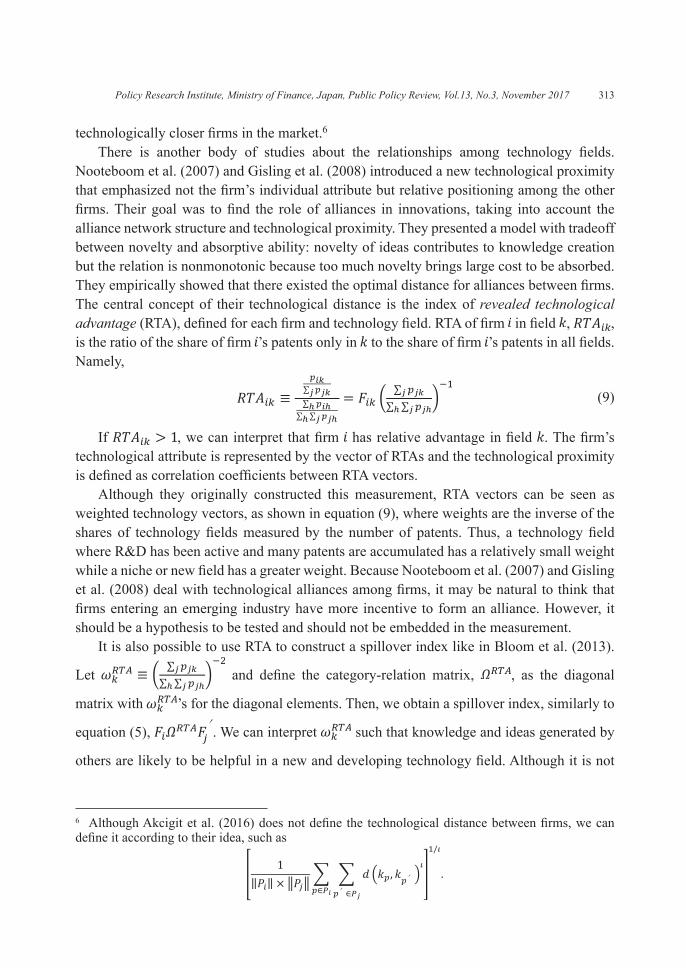
technologically closer firms in the market.6There is another body of studies about the relationships among technology fields.

Nooteboom et al. (2007) and Gisling et al. (2008) introduced a new technological proximity that emphasized not the firm’s individual attribute but relative positioning among the other firms. Their goal was to find the role of alliances in innovations, taking into account the alliance network structure and technological proximity. They presented a model with tradeoff between novelty and absorptive ability: novelty of ideas contributes to knowledge creation but the relation is nonmonotonic because too much novelty brings large cost to be absorbed. They empirically showed that there existed the optimal distance for alliances between firms. The central concept of their technological distance is the index of revealed technological advantage (RTA), defined for each firm and technology field. RTA of firm in field , , is the ratio of the share of firm ’s patents only in to the share of firm ’s patents in all fields. Namely,

(9)

If , we can interpret that firm has relative advantage in field . The firm’s technological attribute is represented by the vector of RTAs and the technological proximity is defined as correlation coefficients between RTA vectors.

Although they originally constructed this measurement, RTA vectors can be seen as weighted technology vectors, as shown in equation (9), where weights are the inverse of the shares of technology fields measured by the number of patents. Thus, a technology field where R&D has been active and many patents are accumulated has a relatively small weight while a niche or new field has a greater weight. Because Nooteboom et al. (2007) and Gisling et al. (2008) deal with technological alliances among firms, it may be natural to think that firms entering an emerging industry have more incentive to form an alliance. However, it should be a hypothesis to be tested and should not be embedded in the measurement.

It is also possible to use RTA to construct a spillover index like in Bloom et al. (2013).

Let and define the category-relation matrix, , as the diagonal

matrix with ’s for the diagonal elements. Then, we obtain a spillover index, similarly to

equation (5), . We can interpret such that knowledge and ideas generated by

others are likely to be helpful in a new and developing technology field. Although it is not

6 Although Akcigit et al. (2016) does not define the technological distance between firms, we can define it according to their idea, such as


clear why the squared inverses of the shares of fields matter and it should be clarified whether a high truly implies a developing category because it may be just an inactive field in terms of patenting, the spillover index with RTA gives us an opportunity to consider inside circumstances of technology fields, which relates to Section III. In Section III, I adjust spillover indexes by incorporating changes within technology fields, which is captured by patent citation overlaps, illustrated in the next subsection.

II-3. Patent Citation Overlaps

Stuart and Podolny (1996) constructed a technological distance by using patent citationoverlaps, which does not depend on technology vectors. Citations are often used to represent knowledge transmission between inventors or firms but they are also informative when we examine in what extent the R&D trajectories of firms are similar because citations tell us the basis of their research. The following example summarizes the technological distance of Stuart and Podolny (1996). Figure 3 depicts citing actions of firms A-C to patents 1-6 by arrows.

They construct a community matrix that represents interfirm relationships. Elements of a community matrix are the indicators that indicate to what degree other firms occupy the fields in which the current firm does research. In Figure 3, out of three citations by firm A (patents 1, 2, 3), only patent 3 is cited by firm B. Then, firm B occupies firm A’s territory at

the rate of . Call this number as . This overlap concept is asymmetric. From firm B’s

point of view, because one of four citations of firm B is cited by firm A. The community matrix collects these rates (with 0 for the diagonal elements) such as

Figure 3. Example of citation overlaps in Stuart and Podolny (1996)


_______

　　

(10)

The first row in equation (10) shows to what degree the other firms occupy firm A’s territory. On the other hand, the first column shows to what degree firm A occupies the territories of the others. The combined vector of the first row and the first column is considered to stand for the technology attribute of firm A. Stuart and Podolny (1996) defined technological distances from those vectors, but it does not seem natural when we consider the meaning of citations in technological relationships among firms. According to their definition, the technological distance between two firms is defined by relationships with the third firms. In the above example, the distance between firms A and B, , is determined by the relation with firm C such that

(11)

Intuitively, it measures the similarity of relationships of the concerned firms with other firms. This idea is convenient to locate firms on a technological space. However, it looks confusing as a concept of distance when we consider the following case. Suppose that firm A cites patent 4 instead of 2 in Figure 3 (no other changes). Then, remains unchanged because only the change in the community matrix is the relation between firms A and B (

and increase to and , respectively). Whereas the common citations between firms A

and B increase, the distance between the two is kept constant because it only compares the relationship with the third party company. On the other hand, suppose that firm A newly cites patent 4 in addition to the original three citations. In this case, we have and

, leading to , its minimum value, even though the citation overlaps are still partial. How do we interpret equation (11) as a technological distance with these examples?

Based on patent citation overlaps, Kitahara and Oikawa (2016) suggest a new technological distance among firms. Figure 4 illustrates how citation overlaps are counted in their definition. Suppose that, in a fixed time period, firm cited patent in squares and firm cited patents in circles. The duplication of cited patents occurs because some patents are repeatedly cited by the same firm when it applies multiple patents in the concerned period. This repetition should not be ignored because frequency of citation indicates the importance of the technology included in the patent for the firm. The degree of citation overlaps in Kitahara and Oikawa (2016) is basically the ratio of the number of the common citations (with duplication) between firms and to the total number of citations. We call this basic fraction as the first-order overlaps. In the example in Figure 4, the first-

order overlaps is . The first-order overlaps only consider the direct relationship between the


two citation lists, but there could be an indirect relationship at the citations-of-citations level. There are two indirect relationships in the current example: patent 2 cited by firm cites patent 5, which is cited by firm ; patent 4 cited by firm cites patent 6 which is cited by patent 5 cited by firm . We put these indirect relationships together in the second-order overlaps and define the degree of citation overlaps as the sum of first- and second-order overlaps with a weight (the second-order overlap is weighted by a positive number less than 1). The technological proximity constructed from the current degree of citation overlaps is in between 0 and 1, where 1 indicates the closest. Unlike Stuart and Podolny (1996), more overlaps lead to more proximity and the highest value, 1, only occurs when the citation lists coincides except for the number of duplications. We consider the second-order level because there are many pairs of firms with no direct overlaps between their citation lists. Taking second- or third-order overlaps, we obtain meaningful degrees of citation overlaps at least for the US patent dataset. Because the generations of patents are finite, we can count overlaps for full order. However, we calculate up to the second-order from the viewpoint of computational burdens.7

Kitahara and Oikawa (2016) defined the technological proximity based on patent citation overlaps to see the locations of firms within technology fields. If we fix technological classification and use technology vectors associated with the classification, heterogeneity within a field is ignored whereas there are various types of R&D in one field. Kitahara and

7 In the United States, an applicant who did not disclose prior arts will lose all right about the concerned patent. This explicit punishment leads to more patent citations other than the examiner’s ones. Thus it is relatively easy to analyze citation overlaps. Because, in Japan and Europe, disclosure of preceding technologies is recommended but there are no punishments, the number of citations are relatively small, compared to the United States.

Figure 4. Example of citation overlaps by Kitahara and Oikawa (2016)


Oikawa (2016) estimated the firm distributions on technology spaces within fields and examined how competition between technology groups in a technology field affects the total amount of innovations.

III. Patent Portfolios and Citation Overlaps within Technological Fields:Estimation of the Spillover Coefficient on Innovations

In this Section, I first observe the dynamic behaviors of the average technologicalproximities and distances surveyed in the previous section by using the US patent data. Based on the observations, I examine the changes in the spillover indices using the traditional measurements with technology vectors. In Section III-2, I incorporate information from citation overlaps and show that the extant method with technology vectors underestimates the impact of knowledge spillovers.

III-1. Spillover index from technological proximity by technology vectors

The dataset I use in this section is the NBER-USPTO patent dataset. It contains about 3.3million patents registered in the USPTO from 1976 to 2006, with the citation list for each patent.8 It tracks changes of patent holders so that we can specify the original applicants. I focus on the patents applied by listed firms in the United States, which narrows the sample of patents to about a half of the full sample.

I use 420 3-digit classes for technology fields which are defined by the USPTO. So the dimensions of technology vectors are 420. I calculate the technology vector for each firm with moving 9-year windows (the first window is 1976-1984, the second one is 1977-1985, and so on). For each 9-year window, I count the number of patent applications for each field for all firms which applied at least one patent during the 9 years, and create technology vectors from dividing it by the total number of firm-level patent applications during the period. I consider moving windows because a firms’ technological attributes should change over time.

From these technology vectors, Figure 5 shows the time-series of averages of Jaffe’s proximity, Jaffe covariance, correlation coefficient, and min-complement distance.9 All technological proximities show upward trends. In particular, it is outstanding around 1990. It may be related with the major patent reform in the US, which promotes pro-patent policies, starting in the early 1980s. Kitahara and Oikawa (2016) also used the year of 1990 as the threshold year of structural change.

The increase in average proximity has an important implication. Based on the model of knowledge transmission in Bloom et al. (2013), an increase in technological proximity leads

8 See Hall et al. (2001) for more details.9 If we use Euclidean distance, technological distances are increasing because of its property mentioned in the previous section.


to an increase in spillovers because knowledge transmission is more likely to occur when the technological backgrounds of a matched pair of researchers are closer. Thanks to the positive externality from spillovers, firms in an environment with higher average proximity tend to innovate more after R&D investments are controlled. To examine this aspect, I estimate the contribution of the spillover index to the number of new patents, following the procedures of Jaffe (1986) and Bloom et al. (2013).

Firm-level R&D stocks, , are estimated as the accumulation of R&D investments by the perpetual inventory method with the depreciation rate of 15%, as in Bloom et al. (2013). For simplicity, I ignore the relationship between technology fields and define Jaffe covariance defined in equation (6) as

(12)

where is the technology vector during the period centered at year because we define technology vectors over 9 years.10 The dependent variable is forward-citation weighted

10 The data on R&D investments are taken from Compustat. I omitted firms that did not report R&D investment for more than 5 years. The number of firms after this omission is 907.

Figure 5. Time-series of several average technological proximities/distances

1975 1980 1985 1990 1995 20000.018

0.02

0.022

0.024

0.026

0.028Jaffe proximity

1975 1980 1985 1990 1995 20005

6

7

8

9

10

11× 10-3 Jaffe covariance

1975 1980 1985 1990 1995 20000.01

0.012

0.014

0.016

0.018

0.02Correlation coef�cient

1975 1980 1985 1990 1995 20001.96

1.962

1.964

1.966

1.968

1.97

1.972

1.974Min-complement


number of patent application (only those granted later), .11 The explanatory variables are the firm-level research input variables in the previous year such as the spillover index, , R&D capital stock, , patent stock, , and flow R&D investment, . Patent stock

is the accumulation of with the depreciation rate of 15% again. The estimation equation is the following.

(13)

Because citation-weighted patents are count numbers and its distribution tends to have a heavy tail, I use the negative binomial regression. Year dummies and primary industry dummies (according to 4-digit SIC codes) are also included in the estimation.

Dividing the sample periods into two at 1990, when the structural shift by pro-patent reforms became obvious, I ran the regressions for both sample periods separately. Columns (1) and (2) in Table 1 show the estimation results with using Jaffe covariance as the spilloverindex. As shown in Table 1, the coefficient for the spillover index is significantly positive inthe former period but becomes insignificant in the latter. The coefficients for other variablesare relatively stable. R&D investment in the previous year positively affects the number ofnew quality-adjusted patents. The knowledge stocks, represented by patent stock and R&Dcapital stock, have opposite signs, which can be interpreted that R&D productivity, measured

11 Citation-weighted patents are often used for quality adjustment because it is convenient but controversial (cf. Bessen, 2008). The other methods use, for example, data on the payment status of patent maintenance fees, and the number of countries to which the same patent is applied.

Table 1. Estimation of the spillover index.


by the patents to investments ratio, matters positively. Columns (3) and (4) repeat the same regressions with adjusting a bias associated with the

number of forward citations. Since later patents have less opportunity to be cited, quality of a new patent tends to be undervalued. To deal with this bias, Hall et al. (2001) calculates a weight as the predicted number of forward citations from the observed distribution of them (called HJT weight). With recalculated and using HJT weights, the regression results show that those in columns (1) and (2) do not depend on the bias of forward citations.

Because the average technological proximity increased during the sample periods as depicted in Figure 5, the spillover index also tends to increase. Then, the result that the coefficient for spillover declines in the above regression implies that increase in knowledge spillovers does not contribute to the amount of new innovations. This is problematic because the socially optimal R&D investment is affected by the size of positive externality stemming from spillovers. If the positive externality is vanishing, there is no economic sense for the government to subsidize private R&D. But did the spillover effects really vanish? Or did they just become difficult to see from the patent data? It is plausible when noticing the controversy that too much pro-patent reforms have damaged the quality of the patent system in the United States (see Jaffe and Lerner, 2004 and Boldrin and Levine, 2008).

To investigate the change of the spillover index more deeply, I will consider changes inside of technology fields in the next subsection, which are neglected when we use technological proximities based on technology vectors.

III-2. Adjustment by Proximity within Fields using Patent Citation Overlaps

Technological proximity/distance based on patent citation overlaps can be definedindependent of technology fields. Here I use the degree of citation overlaps introduced by Kitahara and Oikawa (2016), illustrated in Section II-3. I calculated the technological proximities between firms inside of each technology field for each 9-year window. Figure 6 plots the time-series of the average proximity, where the vertical axis is the average proximity relative to that for the 9-year window of 1990-1998 and the horizontal axis is the initial years of 9-year windows. The figure first tells us that within-field technological proximity is changing over time with about 40% difference from the max to the min. Second, there is no upward or downward trend unlike technological proximities and distances based on technology vectors. Further, the proximity based on citation overlaps has relatively lower values around 1990 whereas the average proximity based on technology vectors surged in those years.

The model of knowledge transmission in Bloom et al. (2013) introduced in Section II-2 helps us interpret Figures 5 and 6. While a company researcher randomly meets another researcher and if they are experts in relatively closer technological fields, then knowledge transmission more likely occurs. However, even though they are in the same technological field, if the field is segmented at deeper levels which is not considered by the extant classification, then the likelihood that they have useful knowledge for one another could be


very small. To take into account this factor in the current regression, I redefine a spillover index by assigning within-field proximity to elements of matrix introduced in equation (5). Neglecting inter-field relationships for simplicity, I define a new technological proximity as an extended version of Jaffe covariance, which I call adjusted Jaffe covariance, ,

(14)

where is the average technological proximity within field . The associated spillover index is

(15)

Table 2 summarizes the estimation results using the spillover index adjusted by average within-field proximity, . As seen in Columns (1) and (2), the coefficients for the adjusted spillover index is higher than in the previous results with the unadjusted spillover index, and it is significantly positive in both groups of periods whereas the coefficient in the latter periods is insignificant in Table 1. Columns (3) and (4), which considers HJT weights for adjustment of patent quality, show similar results.

Because the coefficient of the adjusted spillover index is still lower in the latter period, the decline in the coefficient seen in Table 1 is not fully explained by the changes in within-field proximities. But we can see that the positive externality effect from knowledge spillovers remains significant. Probably, in technology fields in which technological proximity based

Figure 6. Time-series of relative average proximity based on citation overlaps (the base 9-year window is 1980-1998)

1975 1980 1985 1990 1995 20000.95

1

1.05

1.1

1.15

1.2

1.25

1.3

1.35

1.4

1.45

Ave

rage

rel

ativ

e p

roxi

mity


on technology vectors rises, within-field proximity based on citation overlaps decreases. In other words, while allocations of R&D resources getting similar among firms, they are making distinctions from one another in each technology field to win competitions. Then, the unadjusted spillover index is overestimated and, thus, the spillover coefficient is underestimated.

The implication of the current results is the following. First, the spillover coefficient is underestimated unless we take into account within-field proximities. It is important when we consider innovation or growth policies because such underestimation is equivalent to underestimation of the social value of R&D. Second, we need to investigate a decrease in within-field proximity could be caused by segmentation of technology, emergence of a novel field of technology, or competition among technology groups which are based on distinct but substitutable base technologies (Kitahara and Oikawa, 2016). Because those factors may affect R&D productivity and incentives to innovate, it is needed for obtaining an accurate spillover coefficient to know the relationship between firms’ R&D strategies and dynamic changes in within-field proximities, which is a future research topic.

REFERENCES

Aharonson, Barak S. and Melissa A. Schilling (2016), “Mapping the Technological Landscape: Measuring Technology Distance, Technological Footprints, and Technology Evolution,” Research Policy, Vol.45, No.1, pp.81-96.

Table 2. The estimation with the spillover index adjusted by average within-field proximity


Akcigit, Ufuk, Murat A. Celik, and Jeremy Greenwood (2016), “Buy, Keep or Sell: Economic Growth and the Market for Ideas,” Econometrica, Vol.84, No.3, pp.943-984.

Bar, Talia and Aija Leiponen (2012), “A Measure of Technological Distance,” Economics Letters, Vol.116, No.3, pp.457-459.

Benner, Mary and Joel Waldfogel (2008), “Close to You? Bias and Precision in Patent-based Measures of Technological Proximity,” Research Policy, Vol.37, No.9, pp.1556-1567.

Bessen, James (2008), “The Value of U.S. Patents by Owner and Patent Characteristics,” Research Policy, Vol.37, No.5, pp.932-945.

Bloom, Nicholas, Mark Schankerman and John van Reenen (2013), “Identifying Technology Spillovers and Product Market Rivalry,” Econometrica, Vol.81, No.4, pp.1347-1393.

Boldrin, Michele and David K. Levine (2008), Against Intellectual Monopoly, Cambridge University Press.

Cohen, Welsey M., Richard R. Nelson, and John Walsh (2000), “Protecting their Intellectual Assets: Appropriability Conditions and Why U.S. Manufacturing Firms Paten (or Not),” NBER Working Paper 7552.

Gilsing, Victor, Bart Nooteboom, Wim Vanhaverbeke, Geert Duysters, and Ad van den Oord (2008), “Network Embeddedness and the Exploration of Novel Technologies: Technological Distance, Betweenness Centrality and Density,” Research Policy, Vol.37, No.10, pp.1717-1731.

Hall, Bronwyn H., Adam B. Jaffe, and Manuel Trajtenberg (2001), “The NBER Patent Citation Data File: Lessons, Insights and Methodological Tools,” NBER Working Paper 8498.

Jaffe, Adam B. (1986), “Technological Opportunity and Spillovers of R&D: Evidence from Firms’ Patents, Profits, and Market Value,” American Economic Review, Vol.76, No.5, pp.984-1001.

Jaffe, Adam B. and Josh Lerner (2004), Innovation and Its Discontents: How Our Broken Patent System is Endangering Innovation and Progress, and What to Do About It, Princeton University Press.

Jones, Charles I. and John C. Williams (1998), “Measuring the Social Return to R&D,” Quarterly Journal of Economics, Vol.113, No.4, pp.1119-1135.

Kitahara, Minoru and Koki Oikawa (2016), “Technology Polarization,” mimeo.Kortum, Samuel (1997), “Research, Patenting, and Technological Change,” Econometrica,

Vol.65, No.6, pp.1389-1419. Nagaoka, Sadao, Kazuyuki Motohashi, and Akira Goto (2010), “Patent Statistics as an

Innovation Indicator,” Handbook of the Economics of Innovation Vol.2, Elsevier, pp.1083-1128.

Nemet, Gregory F., and Evan Johnson (2012), “Do Important Inventions Benefit from Knowledge Originating in Other Technological Domains?” Research Policy, Vol.41, No.1, pp.190-200.

Nooteboom, Bart, Wim Van Haverbeke, Geert Duysters, Victor Gilsing, & Ad van den Oord (2007), “Optimal Cognitive Distance and Absorptive Capacity,” Research Policy,


Vol.36, No.7, pp.1016-1034. Rosenkopf, Lori and Paul Almeida (2003), “Overcoming Local Search Through Alliances

and Mobility,” Management Science, Vol.49, No.6, pp.751-766.Stuart, Toby E. and Joel M. Podolny (1996), “Local Search and the Evolution of Technological

Capabilities,” Strategic Management Journal, Vol.17, No.S1, pp.21-38.Thomasello, Napoletano, Garas, and Schweitzer (2016), “The Rise and Fall of R&D

Networks,” ISI Growth Working Paper.


Inter-firm Technological Proximity and Knowledge Spillovers › english › pri › publication ›...

Documents

Transcript of Inter-firm Technological Proximity and Knowledge Spillovers › english › pri › publication ›...