Intentionally Blank Slide

Superconductivity & Power Cables

Paul M. GrantVisiting Scholar in Applied Physics, Stanford

UniversityEPRI Science Fellow (retired)

IBM Research Staff Member EmeritusPrincipal, W2AGZ Technologies

w2agz@pacbell.netwww.w2agz.com

EPRI Workshop on SCDC Cables12 - 14 October 2005, Palo Alto

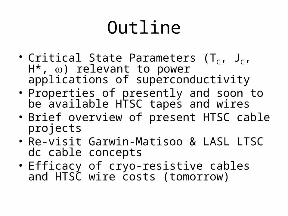
Outline

• Critical State Parameters (TC, JC, H*, ) relevant to power applications of superconductivity

• Properties of presently and soon to be available HTSC tapes and wires

• Brief overview of present HTSC cable projects

• Re-visit Garwin-Matisoo & LASL LTSC dc cable concepts

• Efficacy of cryo-resistive cables and HTSC wire costs (tomorrow)

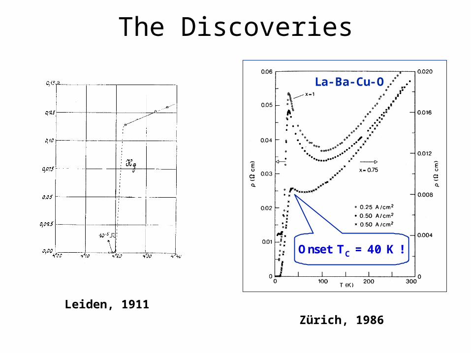
The Discoveries

Leiden, 1911

Onset TC = 40 K !

La- Ba- Cu- O

Onset TC = 40 K !

La- Ba- Cu- O

Zürich, 1986

+ +

+ +•e-

+ +

+ +•e-

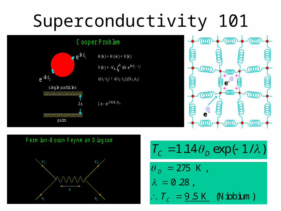
Superconductivity 101C ooper P r ob lem

2

s ingle particles

pairs

e ik r1

e -ik r2

H(k) + H(-k) + V(k)

V(k) = -V0 0 k f dk e ik(r

1 - r

2)

(r1-r2) = (r1-r2)(s 1,s 2)

2 e-2/N(E f)V 0

F er m ion -B oson F eynm an D iagr am

q

k1

k'1

k2

k'2

)/1exp( 14.1 DCT

(Niobium) K 5.9

,28.0

,K 275

C

D

T

)/1exp( 14.1 DCT

(Niobium) K 5.9

,28.0

,K 275

C

D

T

•-• eeee

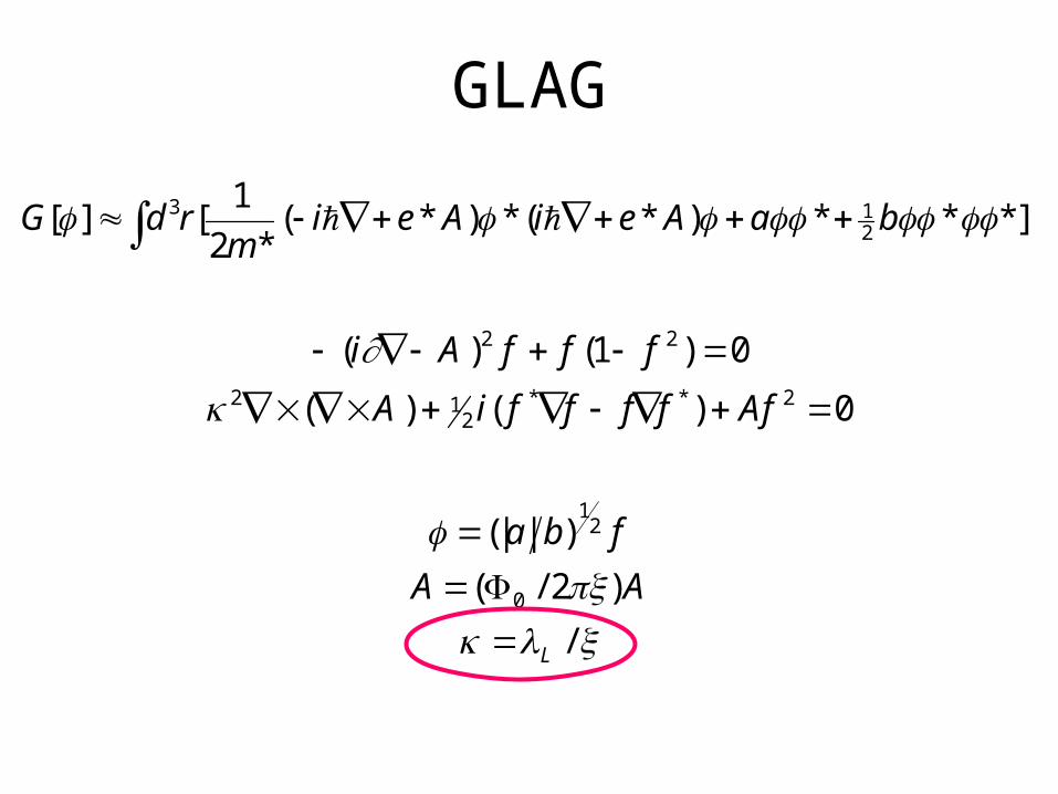
GLAG

G d rm

i e A i e A a b[ ] [*

( * ) *( * ) * * *] 3 12

1

2

( ) ( )

( ) ( )

(| | )

( / )

/

* *

i f f f

i f f f f f

a b f

A

L

A

A A

A

2 2

2 12

2

12

0

1 0

0

2

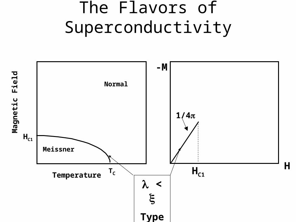
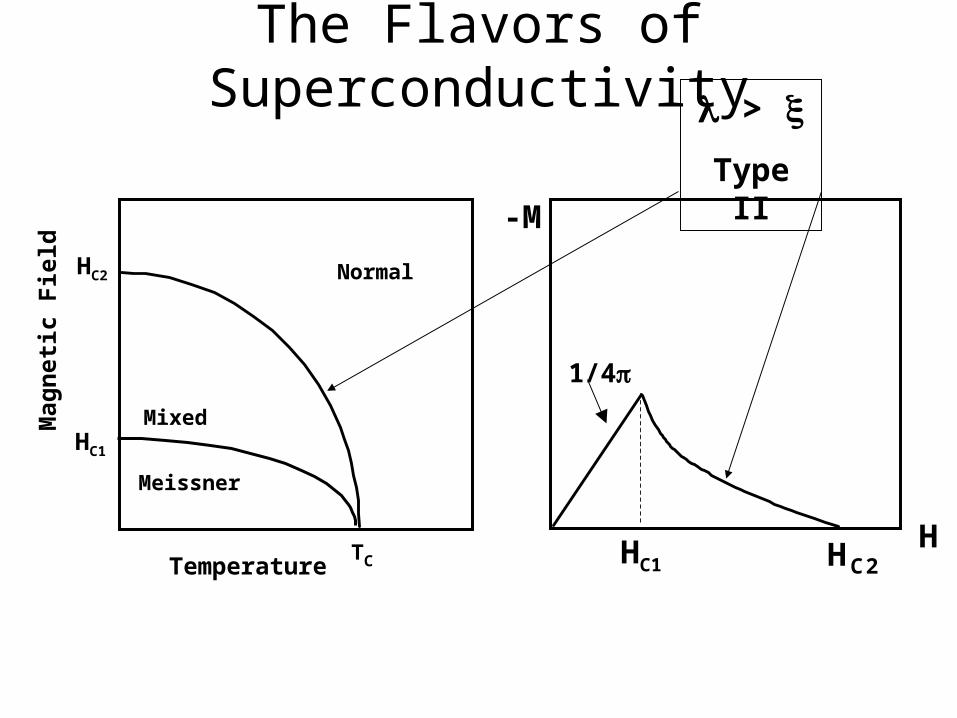
The Flavors of Superconductivity

1/4

HC1H

-M

Meissner

HC1

Normal

TCTemperature

Mag

net

ic F

ield

<

Type I

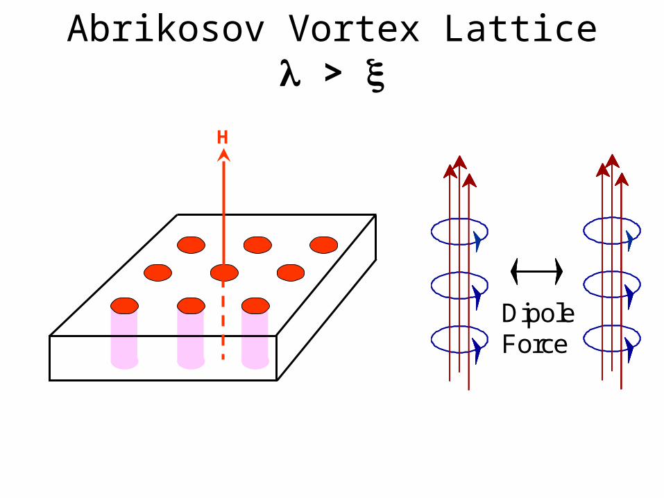
Abrikosov Vortex Lattice >

DipoleForceDipoleForce

H

The Flavors of Superconductivity

1/4

HC1H

-M

Meissner

HC1

Normal

TCTemperature

Mag

net

ic F

ield

HC2

HC2

Mixed

>

Type II

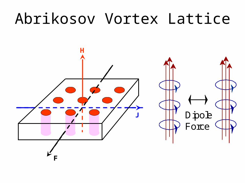
Abrikosov Vortex Lattice

DipoleForceDipoleForce

J

H

FF

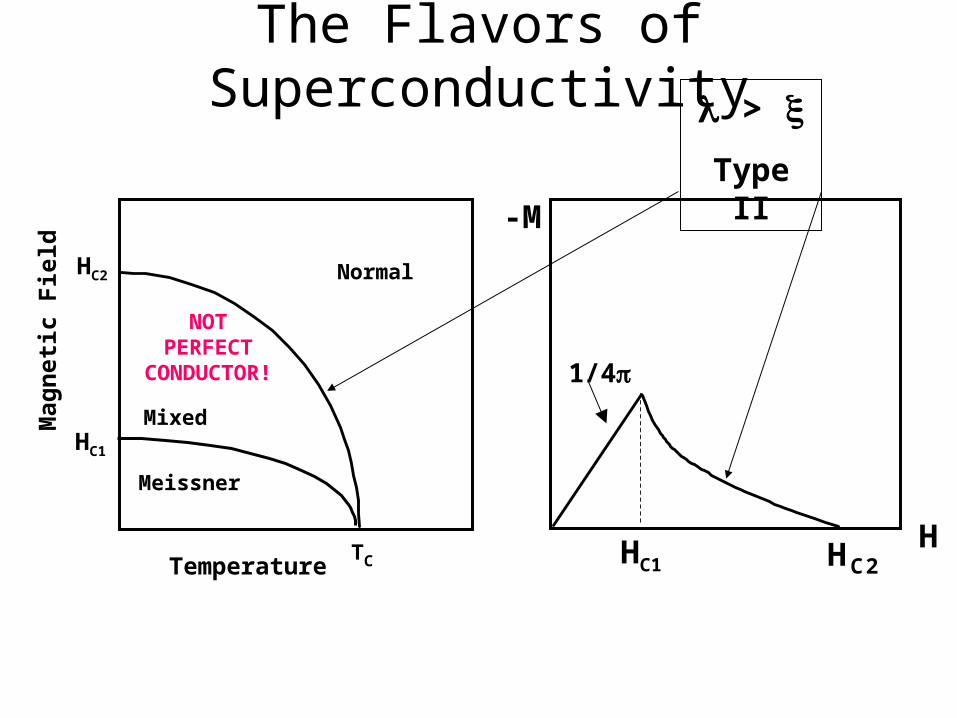
The Flavors of Superconductivity

1/4

HC1H

-M

Meissner

HC1

Normal

TCTemperature

Mag

net

ic F

ield

HC2

HC2

Mixed

>

Type II

NOTPERFECT

CONDUCTOR!

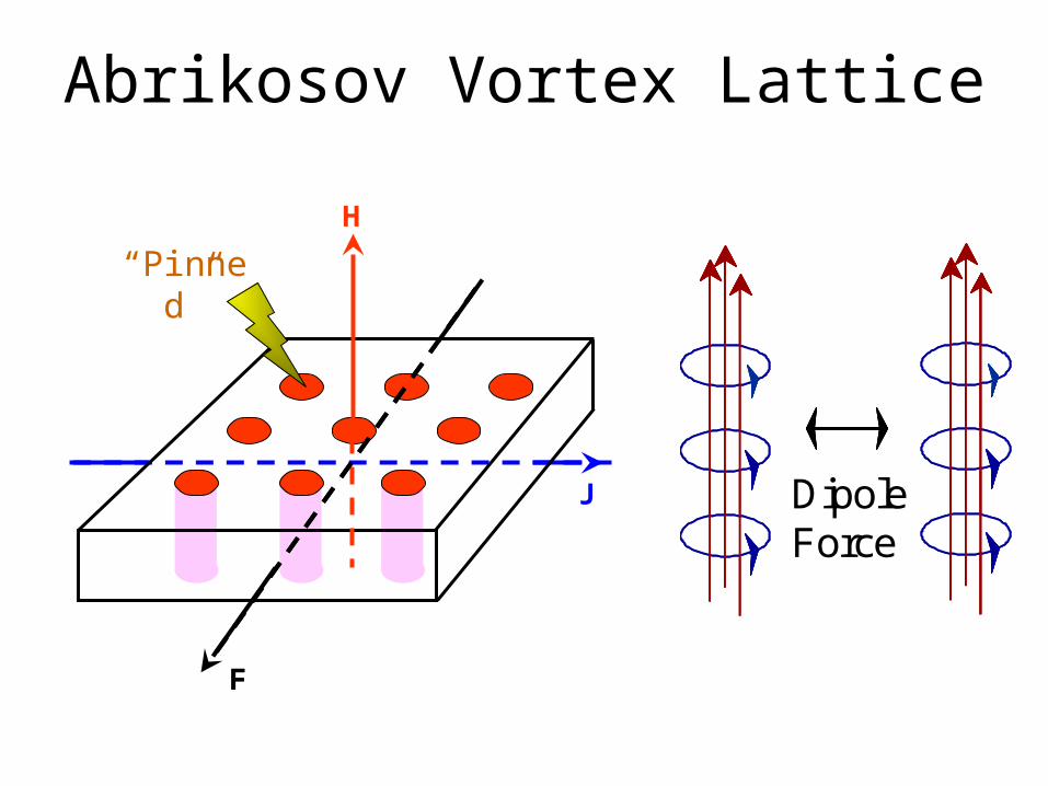
Abrikosov Vortex Lattice

DipoleForceDipoleForce

J

H

FF

“Pinned”

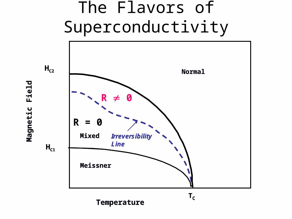
IrreversibilityLineIrreversibilityLine

Meissner

HC1

Normal

TCTemperature

Mag

net

ic F

ield

HC2

Mixed

The Flavors of Superconductivity

R = 0

R 0

Meissner

HC1

Normal

TCTemperature

Mag

net

ic F

ield

HC2

Mixed

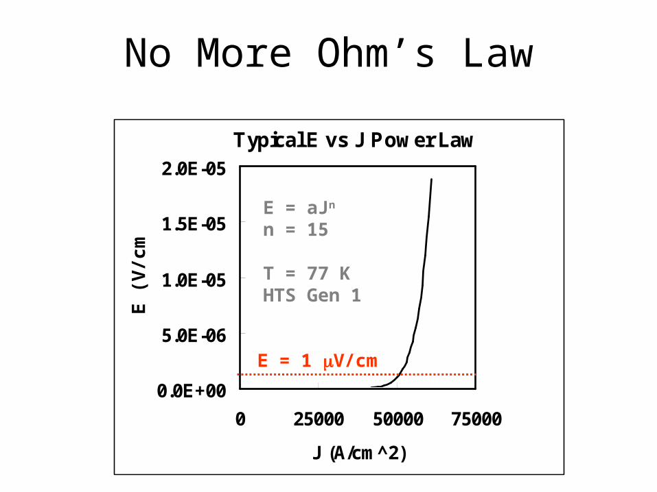
No More Ohm’s Law

Typical E vs J Power Law

0.0E+00

5.0E-06

1.0E-05

1.5E-05

2.0E-05

0 25000 50000 75000

J (A/cm^2)

E (

V/c

m)

E = aJn

n = 15

T = 77 KHTS Gen 1

E = 1 V/cm

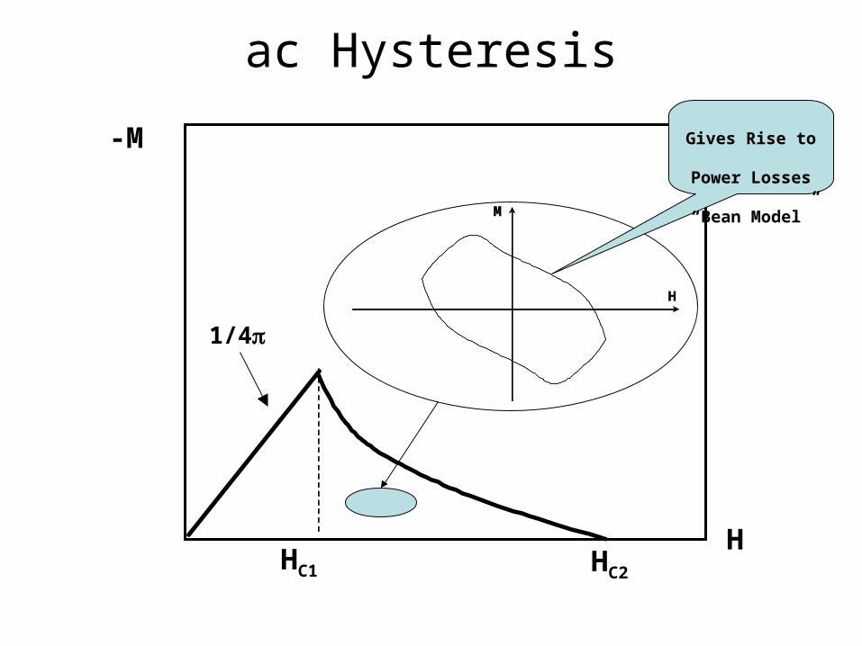
ac Hysteresis

1/4

HC1

H

-M

HC2

H

M

H

M

Gives Rise to

Power Losses

“Bean Model”

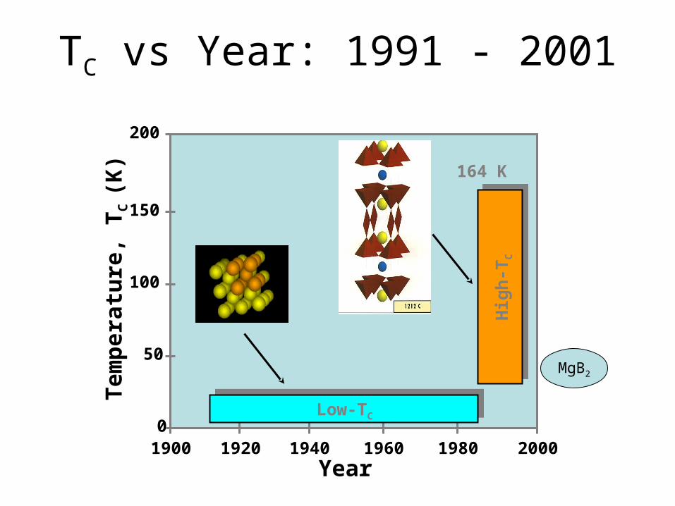
TC vs Year: 1991 - 2001

1900 1920 1940 1960 1980 2000 0

50

100

150

200T

emp

erat

ure

, T

C (K

)

Year

Low-TC

Hig

h-T

C

164 K

MgB2

Oxide Powder Mechanically Alloyed Precursor

1. PowderPreparation

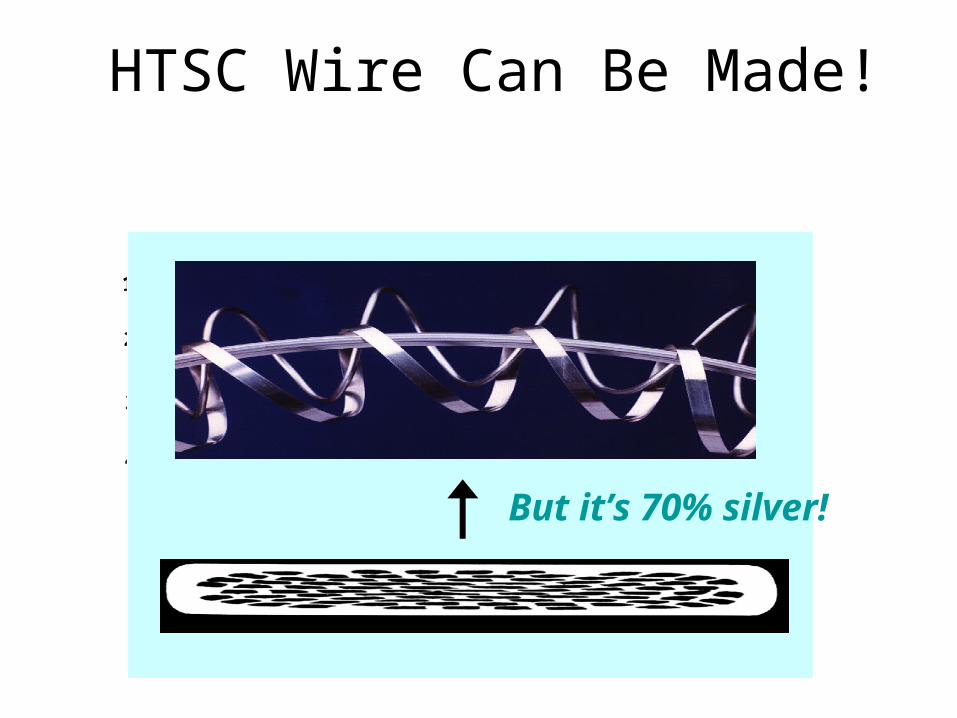
HTSC Wire Can Be Made!

A. Extrusion

B. Wire DrawC. RollingDeformation

& Processing3.

Oxidation -Heat Treat

4.

Billet Packing& Sealing

2.

But it’s 70% silver!

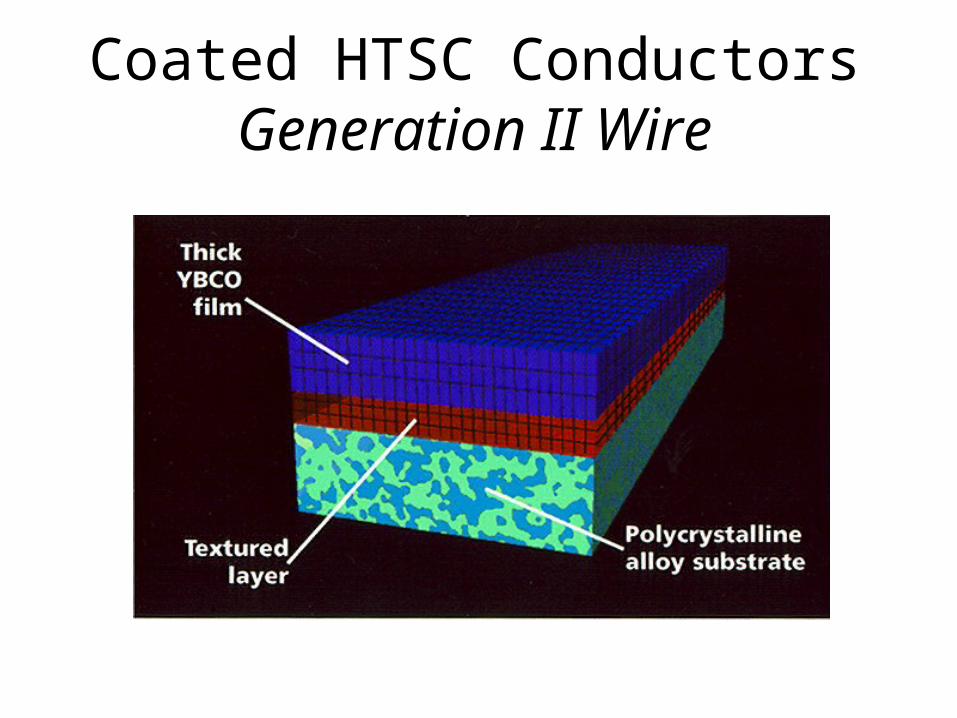
Coated HTSC ConductorsGeneration II Wire

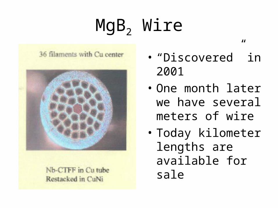
MgB2 Wire

• “Discovered” in 2001

• One month later we have several meters of wire

• Today kilometer lengths are available for sale

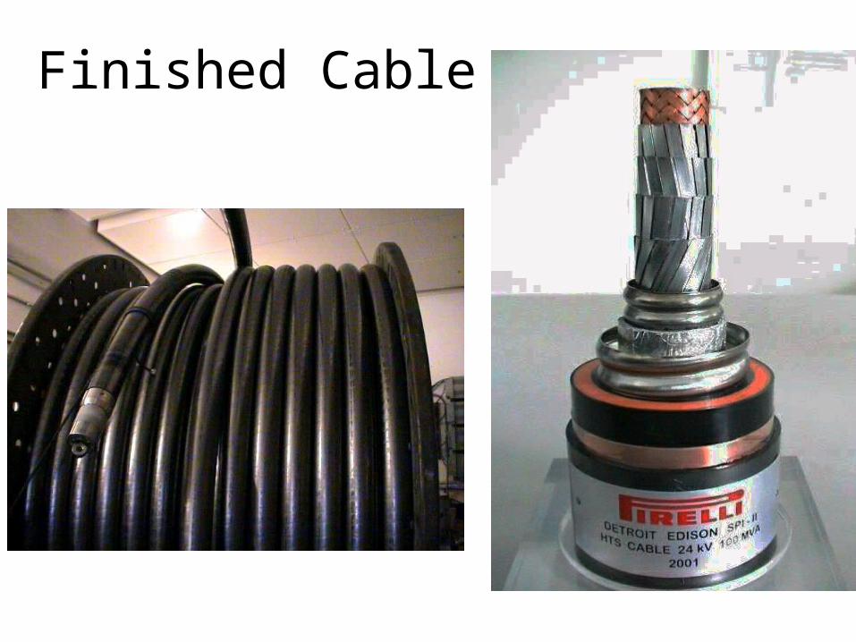
Finished Cable

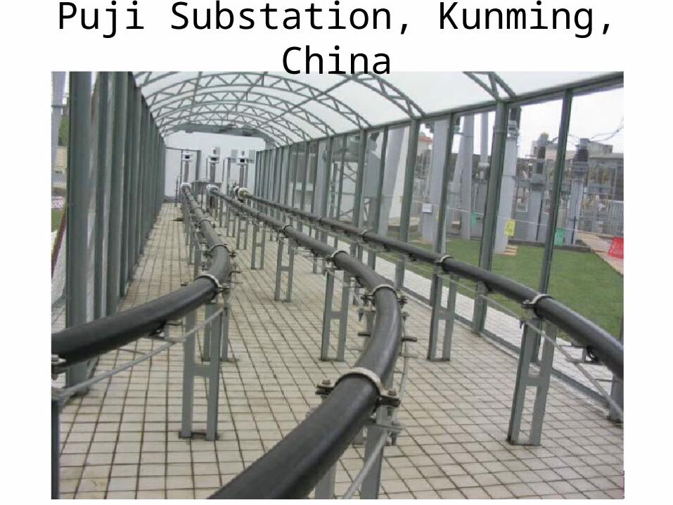
Puji Substation, Kunming, China

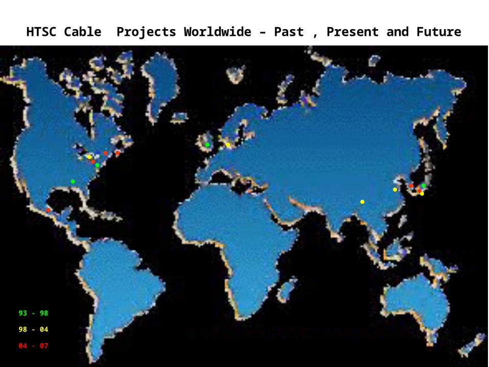
HTSC Cable Projects Worldwide – Past , Present and Future

04 - 07

93 - 98

98 - 04

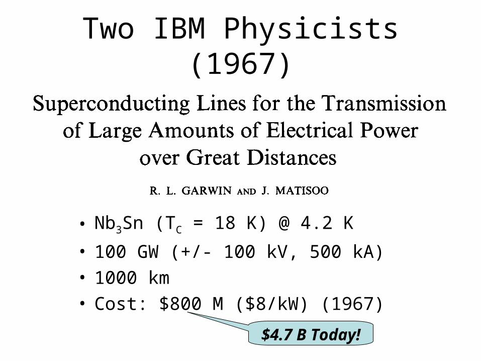
Two IBM Physicists (1967)

• Nb3Sn (TC = 18 K) @ 4.2 K

• 100 GW (+/- 100 kV, 500 kA)• 1000 km• Cost: $800 M ($8/kW) (1967)

$4.7 B Today!

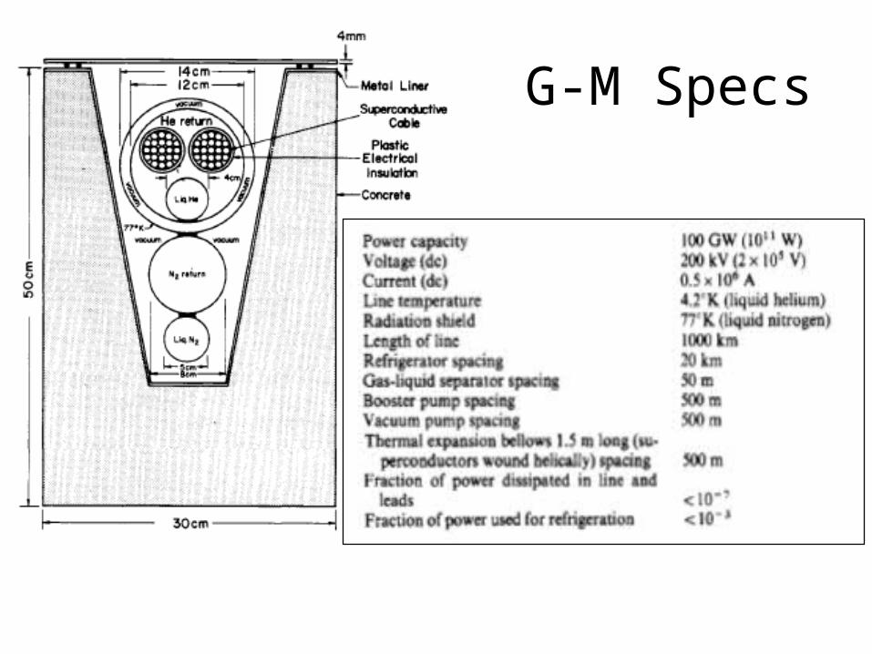
G-M Specs

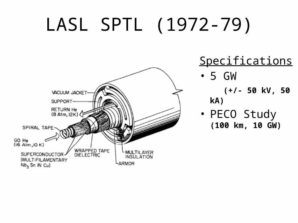
LASL SPTL (1972-79)

Specifications• 5 GW

(+/- 50 kV, 50 kA)

• PECO Study (100 km, 10 GW)

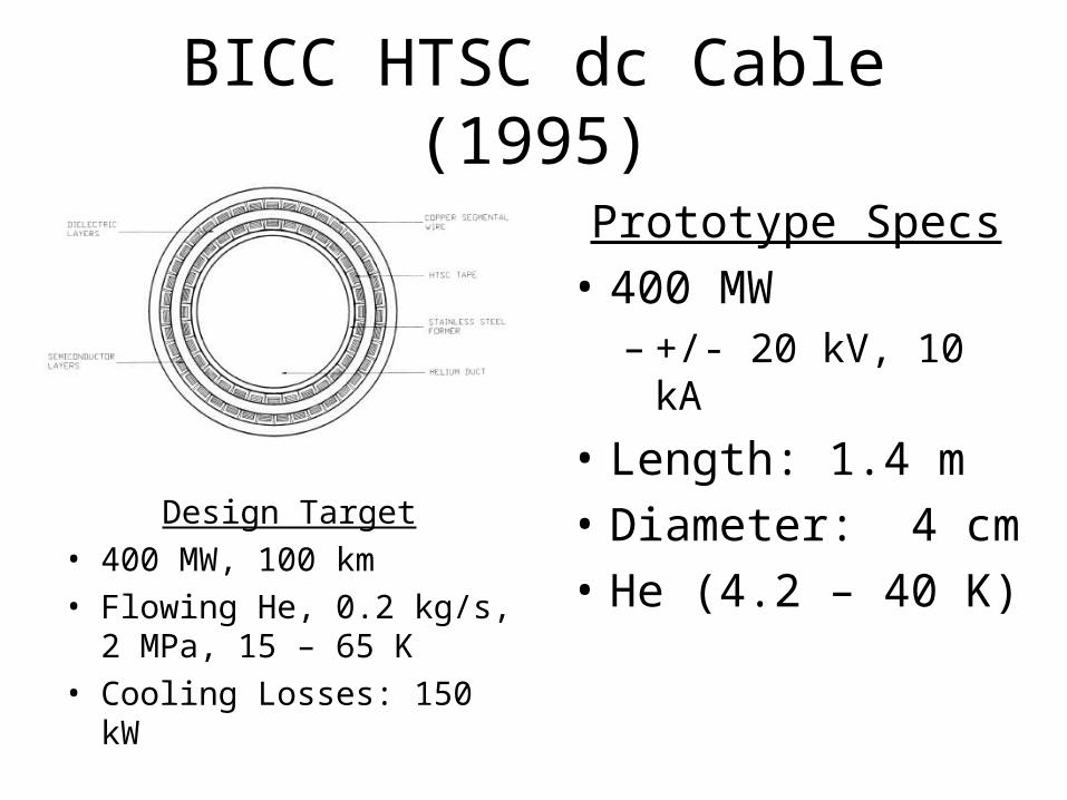
BICC HTSC dc Cable (1995)

Design Target• 400 MW, 100 km• Flowing He, 0.2 kg/s, 2

MPa, 15 – 65 K• Cooling Losses: 150

kW

Prototype Specs• 400 MW

– +/- 20 kV, 10 kA

• Length: 1.4 m• Diameter: 4 cm• He (4.2 – 40 K)

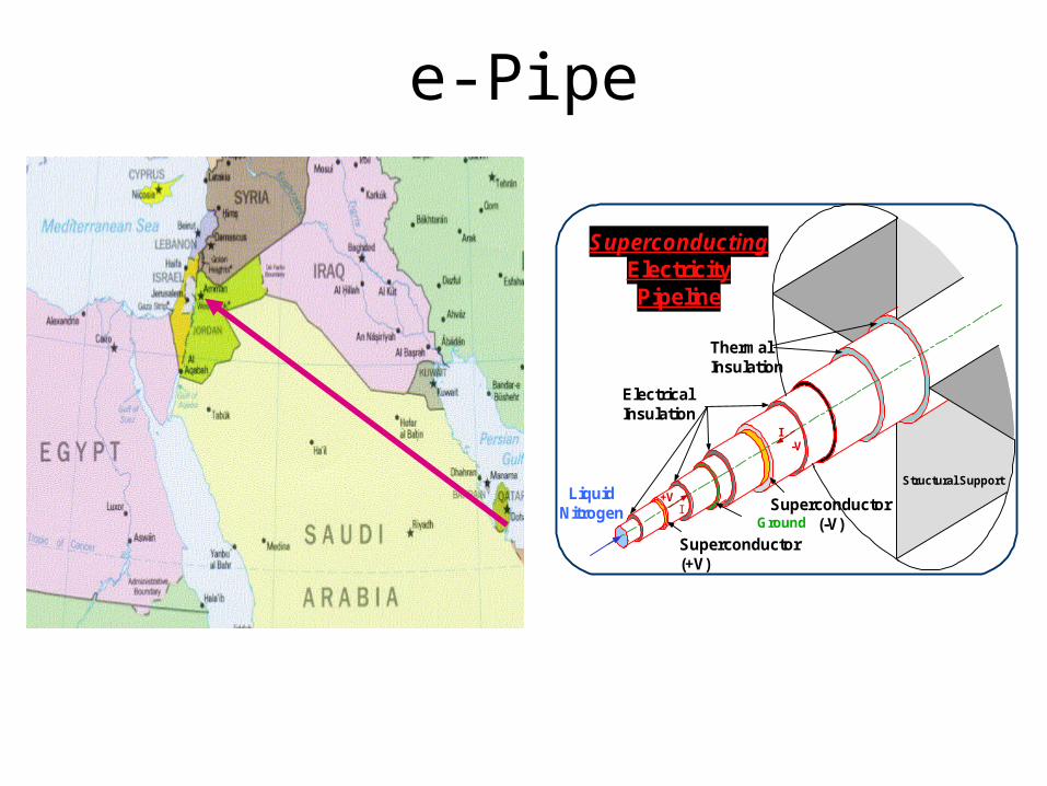
e-Pipe

I-V

Ground

Structural Support

SuperconductingElectricityPipeline

ThermalInsulation

ElectricalInsulation

Superconductor(-V)

Superconductor(+V)

+VI

LiquidNitrogen

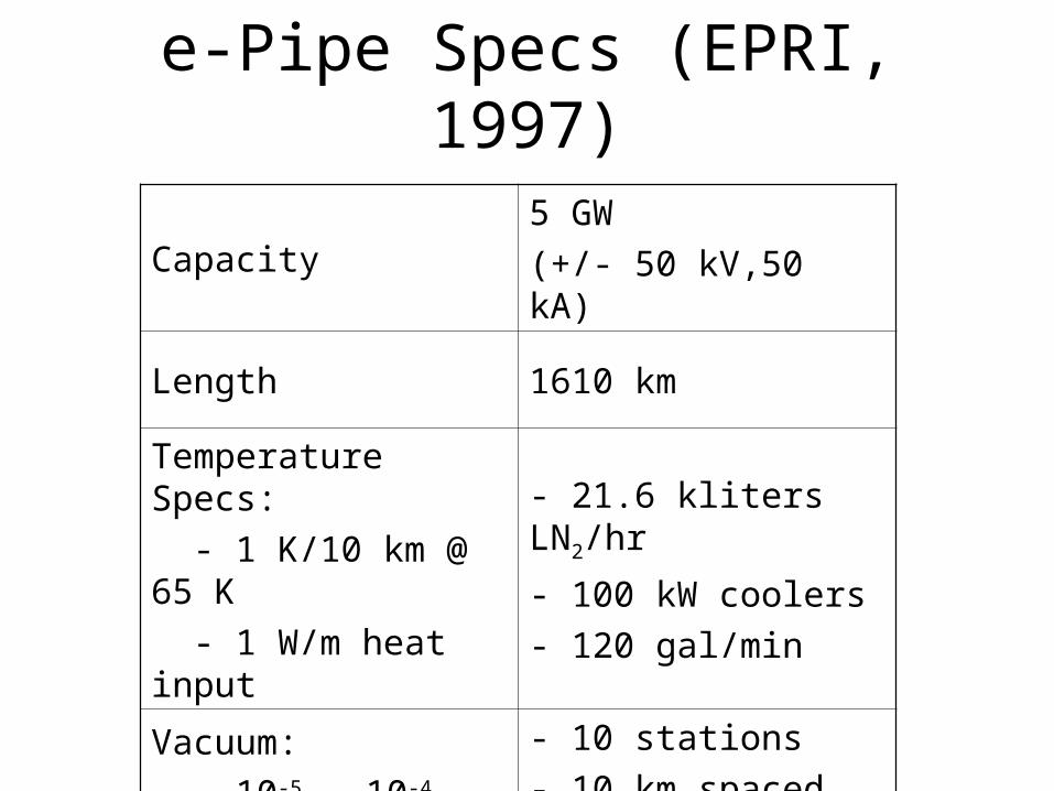
e-Pipe Specs (EPRI, 1997)

Capacity5 GW (+/- 50 kV,50 kA)

Length 1610 km

Temperature Specs: - 1 K/10 km @ 65 K - 1 W/m heat input

- 21.6 kliters LN2/hr

- 100 kW coolers- 120 gal/min

Vacuum: - 10-5 – 10-4 torr

- 10 stations- 10 km spaced- 200 kW each

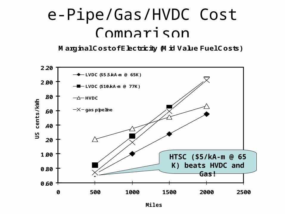
Marginal Cost of Electricity (Mid Value Fuel Costs)

0.60

0.80

1.00

1.20

1.40

1.60

1.80

2.00

2.20

0 500 1000 1500 2000 2500

Miles

c/k

Wh

LVDC ($5.5/kA-m @ 65K)

LVDC ($10/kA-m @ 77K)

HVDC

gas pipeline

e-Pipe/Gas/HVDC Cost Comparison

Marginal Cost of Electricity (Mid Value Fuel Costs)

0.60

0.80

1.00

1.20

1.40

1.60

1.80

2.00

2.20

0 500 1000 1500 2000 2500

Miles

c/k

Wh

LVDC ($5.5/kA-m @ 65K)

LVDC ($10/kA-m @ 77K)

HVDC

gas pipeline

US

ce

nts

/kW

h

Miles

HTSC ($5/kA-m @ 65 K) beats HVDC and Gas!

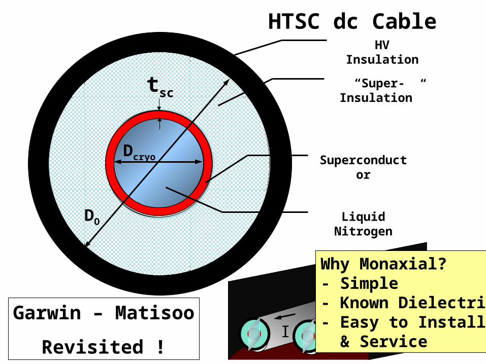
I I

HV Insulation

“Super-Insulation”

Superconductor

Liquid Nitrogen

DO

Dcryo

tsc

HTSC dc Cable

Garwin – Matisoo

Revisited !

Why Monaxial?- Simple- Known Dielectric- Easy to Install & Service

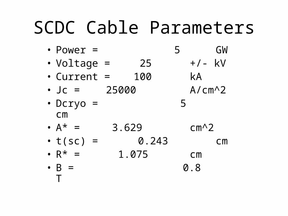
SCDC Cable Parameters• Power = 5 GW• Voltage = 25 +/- kV• Current = 100 kA• Jc = 25000 A/cm^2• Dcryo = 5 cm• A* = 3.629 cm^2• t(sc) = 0.243 cm• R* = 1.075 cm• B = 0.8 T

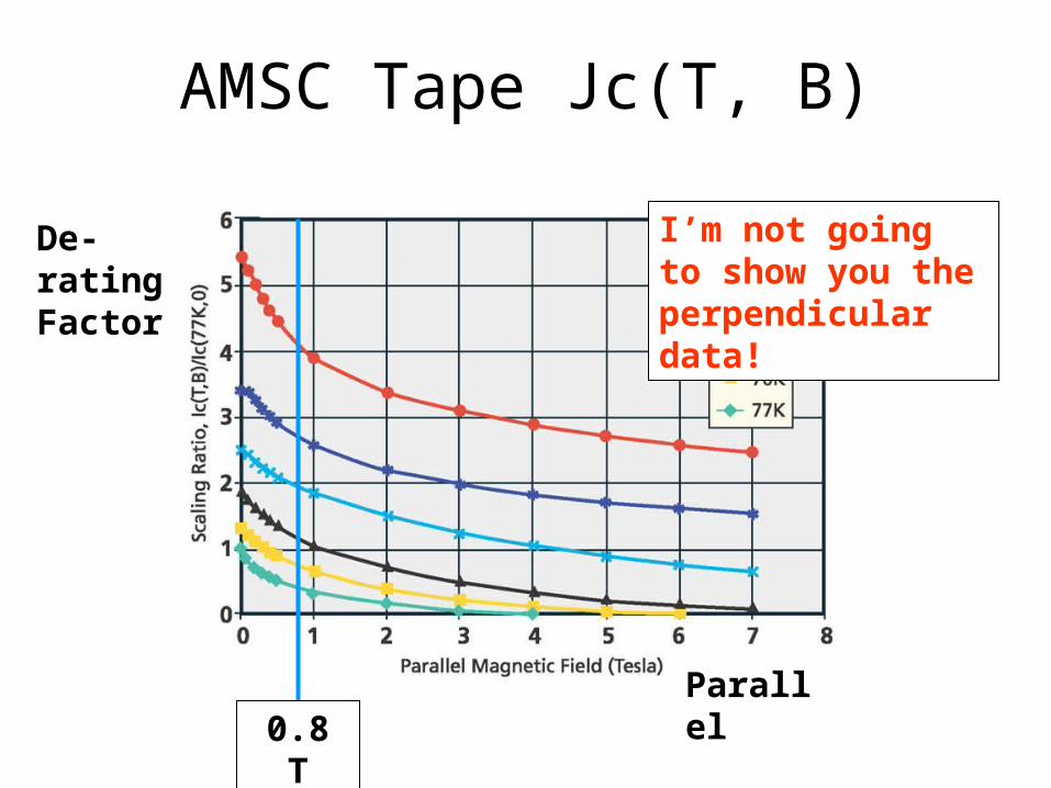
AMSC Tape Jc(T, B)

Parallel

De-ratingFactor

0.8 T

I’m not going to show you the perpendicular data!

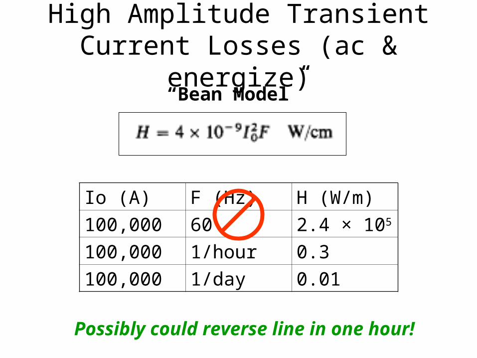
High Amplitude Transient Current Losses (ac & energize)

Io (A) F (Hz) H (W/m)

100,000 60 2.4 × 105

100,000 1/hour 0.3

100,000 1/day 0.01

Possibly could reverse line in one hour!

“Bean Model”

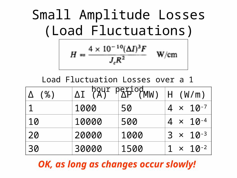
Small Amplitude Losses(Load Fluctuations)

Δ (%) ΔI (A) ΔP (MW) H (W/m)

1 1000 50 4 × 10-7

10 10000 500 4 × 10-4

20 20000 1000 3 × 10-3

30 30000 1500 1 × 10-2

Load Fluctuation Losses over a 1 hour period

OK, as long as changes occur slowly!

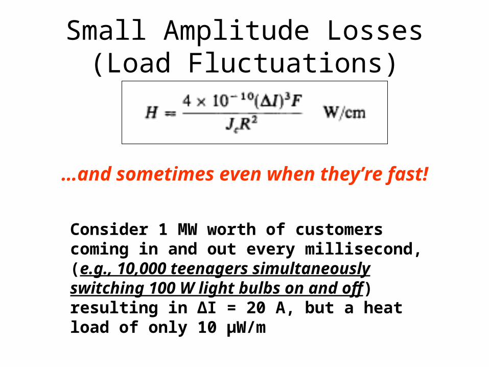
Small Amplitude Losses(Load Fluctuations)

…and sometimes even when they’re fast!

Consider 1 MW worth of customers coming in and out every millisecond, (e.g., 10,000 teenagers simultaneously switching 100 W light bulbs on and off) resulting in ΔI = 20 A, but a heat load of only 10 μW/m

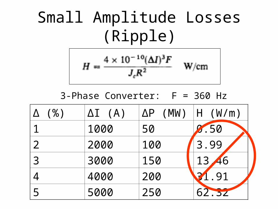
Small Amplitude Losses(Ripple)

Δ (%) ΔI (A) ΔP (MW) H (W/m)

1 1000 50 0.50

2 2000 100 3.99

3 3000 150 13.46

4 4000 200 31.91

5 5000 250 62.32

3-Phase Converter: F = 360 Hz

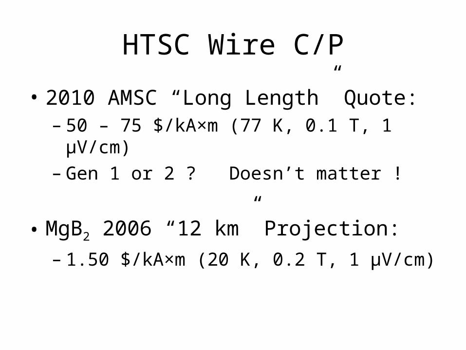
HTSC Wire C/P

• 2010 AMSC “Long Length” Quote:– 50 – 75 $/kA×m (77 K, 0.1 T, 1 μV/cm)– Gen 1 or 2 ? Doesn’t matter !

• MgB2 2006 “12 km” Projection:– 1.50 $/kA×m (20 K, 0.2 T, 1 μV/cm)

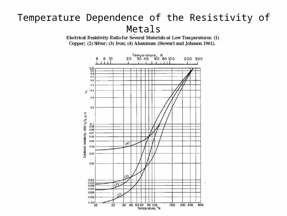
Temperature Dependence of the Resistivity of Metals

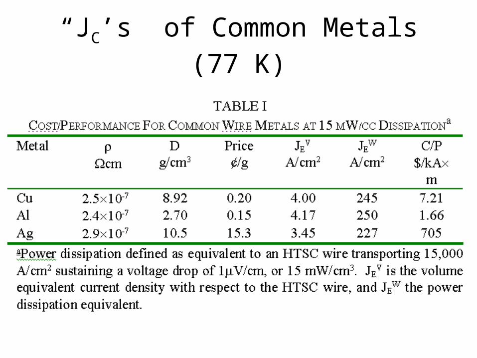
“JC’s” of Common Metals (77 K)

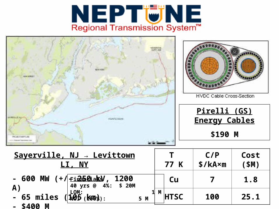
Sayerville, NJ → Levittown LI, NY

- 600 MW (+/- 250 kV, 1200 A)- 65 miles (105 km)- $400 M- 2007

Pirelli (GS)Energy Cables

$190 M

T 77 K

C/P$/

kA×m

Cost ($M)

Cu 7 1.8

HTSC 100 25.1

Financials40 yrs @ 4%: $ 20MLOM: 1 MNOI (100%): 5 M

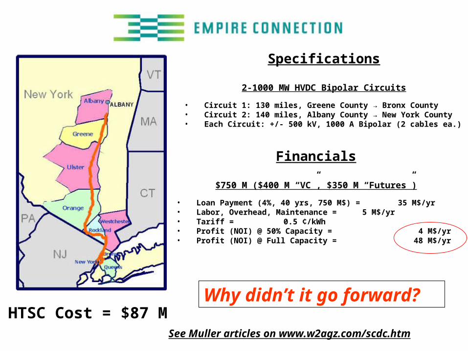
Financials

$750 M ($400 M “VC”, $350 M “Futures”)

• Loan Payment (4%, 40 yrs, 750 M$) = 35 M$/yr

• Labor, Overhead, Maintenance = 5 M$/yr• Tariff = 0.5 ¢/kWh• Profit (NOI) @ 50% Capacity = 4 M$/yr• Profit (NOI) @ Full Capacity = 48 M$/yr

Specifications

2-1000 MW HVDC Bipolar Circuits

• Circuit 1: 130 miles, Greene County → Bronx County• Circuit 2: 140 miles, Albany County → New York County• Each Circuit: +/- 500 kV, 1000 A Bipolar (2 cables ea.)

Why didn’t it go forward?HTSC Cost = $87 M

See Muller articles on www.w2agz.com/scdc.htm

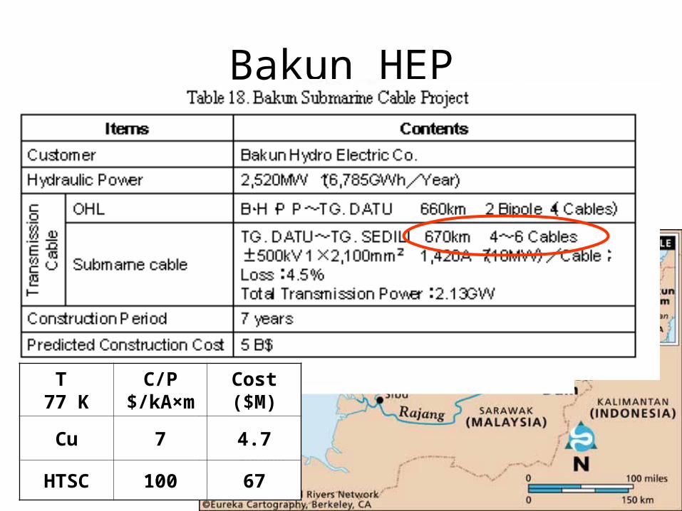
Bakun HEP

T 77 K

C/P$/

kA×m

Cost ($M)

Cu 7 4.7

HTSC 100 67