Intelligent Combination of Structural Analysis Algorithms ...
AD-A267 755RL-TR-93-75 III 11 III II liiIInterim ReportMay 1993
INTELLIGENT USE OF CFARALGORITHMS
Kaman Sciences Corporation
P. Antonik, B. Bowles, G. Capraro, L. Hennington,A.Koscielny, R. Larson (Kaman)M. Uner, P. Varshney, D. Weiner (Syracuse University)
, I, . c'. ViJ = ' N
APPROVED FOR PUB IC REL EA"S DISTRIBUIrON UNLIMITED.
Rome Laboratory
Air Force Materiel Command
93- 18307 ffiss Air Force Base, New York
This report has been reviewed by the Rome Laboratory Public Affairs Office(PA) and is releasable to the National Technical Information Service (NTIS). At NTISit will be releasable to the general public, including foreign nations.
RL-TR-93-75 has been reviewed and is approved for publication.
esfion Tor
DT TAB 0Une Owce
APPROVED: &cstj Gat or
WILLIA-M J. BALDYGO, JR. B7.
Project Engineer DIsjtiributi
AV ilabi t' Godes
Dist speolak\
FOR THE COMMANDER:
JAMES W. YOUNGBERG, Lt Col, USAFDeputy DirectorSurveillance and Photonics Directorate
If your address has changed or if you wish to be removed from the Rome Laboratorymailing list, or if the addressee is no longer employed by your organization, pleasenotify RL(4514 ) Griffiss AFB, NY 13441-4514. This will assist us in maintaining acurrent mailing list.
Do not return copies of this report unless contractual obligations or notices on aspecific document require that it be returned.
DISCLAIMER NOTICE
THIS DOCUMENT IS BEST
QUALITY AVAILABLE. THE COPY
FURNISHED TO DTIC CONTAINED
A SIGNIFICANT NUMBER OF
PAGES WHICH DO NOT
REPRODUCE LEGIBLY.
ArmpprovedREPORT DOCUMENTATION PG 0MBN. 7408P,.k ;uptk~ gu. knole fo* coloilcon d k'f~ammbt Is sid ists toavworo I how pw rmp "uI ft fte fo rdi4 hfluriAbra .mid*V clts~~ @w~ongollwfti widiariarilt~wtig~ de rdesled wd moowrniylw . fr. tuaohadb, Sefnd w acorYwirts Neg~ij b~ed.e sob *W MwyW awuped of ". ,,la d i~Wou ob I .~h OA* agersgt for to WIw g.w .uO ~~u sath poirsti nRopcts.12`16.Jullwa~nUOsVW M~V, SLA*e 14.A*,War VA um4mw, dto U.Ofl~d M,.pwrvut . idz*cP~.waI Rm*d~fiProa (0704X401S, Wais- orDC 29
1. AGENCY USE ONLY (Leave Blank) 2. REPORT DATE 3. REPORT TYPE AND DATES COVERED
IMay 1993 Inte 'rim Jan 92 - Se2 924. TITLE AND SUBTITLE 5. FUNDING NUMBERSINTELLIGENT USE OF CFAR ALGORITHMS C - F30602-91-C-0017
PR - 45066,.AUTHOR($) p. Antonik, B. Bowles, G. Caparo, L. Hennington, TA - 11A. Koscielny, R. Larson (Kaman Sciences Corp), M. liner, W`U - iCP. Varshney, D. Weiner (Syracuse University) __________
7. PERFORMING ORGANIZATION NAME(S) AND ADDRESS(ES) & PERFORMING ORGAN17ATIOiNKaman Sciences Corporation Syracuse Univursity REPORT NUMBER258 Genesee Street Dept of Electrical andUtica NY 13502-4627 Computer Engineering
Syracuse NY 13244-1240
9. SPONSORINGIMONITORING AGENCY NAME(S) AND ADDRESS IS) 10. SPONSORINQIMONITORINGRome Laboratory (OCTS) AGENCY REPORT NUMBER26 Electronic Parkw~y RL-TR-93-75Griffiss APB NY 13441-4514
11 . SUPPLEMENTARY NOTESRome Laboratory Project Engineer: William J. Baldygo, Jr./OCTS/(315)330-4049
1 2a. DISTRIBUTION/AVAILABIU1TY STATEMENT 12b. DISTRIBUTION CODE
Approved for public release; distribution unlimited
13.1/ BSTRACT(mack-n 2w words)The objective of this program is to demonstrate CFAR detection improvement by applyingartificial intelligence techniques. The basic concept is one in which a system thatdynamically selects the most appropriate CFAR algorithms based upon the characteristicsof the interference, out-perform a single, fixed CFAR algorithm. This report describesone prototype Expert System CFAR Processor, its current status, implementation detailsand capabilities. Also discussed are GEAR algorithm testing and evaluation, andrulebase development.
14. SUBJECT TERMS is NUMBER OF PAGES 14Rdar Signal Processing, CFAR Detection, Expert Systems It PRICE CODE 14
17. SECURITY CLASSIFICATION 1I& SECURITY CLASSIFICAT ION 19. SECURITY CLASSIFICATION 20. LIMITATION OF ABSTRACT%EOTOF THIS PAGE OF ABOTRACT /~1CLASSIFIED UNCLASSIFIED UNCLASSIFIED U/
NSN 7540411 21114=0 Stu dwd Form 2W6 (Rev 2-811Prosurbid btV ANSI Std ZgIs

Table of Contents
1.0 Executive Overview 1
2.0 KBS Development 6
2.1 Expert System Development 72.1.1 Expert Systems 102.1.2 Gensym G2 17
2.2 KBS Overview 192.3 Simulated Data 272.4 Implementation of CFAR Algorithms 322.5 Performance Measures 362.6 Testing and Verification of CFAR Algorithms 39
3.0 CFAR Evaluation 51
3.1 Introduction 513.2 Performance Analysis of CFAR Processors
in K-Distributed Clutter 573.2.1 Simulation Procedure 613.2.2 Simulation Results 67
3.2.2.1 Homogeneous Background 673.2.2.2 Non-Homogeneous Background 743.2.2.3 Homogeneous Background With
Different Pf Design Values 99
4.0 Summary of Technical Program Status 114 A
References DTIC QUALITY IN•8C"TF•D 3 118S.o.o. ...... .
Appendix A: Summary of CFAR Literature Search A-1 ......uility Codes
Avail and I -rDist Special
1.0 EXECUTIVE OVERVIEW
This is the second interim report for Contract No. F30602-91-C-0017, entitled
"Intelligent Use of CFAR Algorithms". The primary objective of this effort is to
demonstrate that an expert system CFAR processor, which dynamically selects
CFAR algorithms and their parameters based on the environment, can out-perform
a fixed, single algorithm processor. The primary emphasis of this report is todocument the current status of the Expert System (ES) Constant False Alarm Rate(CFAR) system. This section provides an overview of the ES CFAR program.
Automatic detection schemes are typically employed in operational radarsystems. These circuits automatically declare and record target detections fromreceived signals without human interpretation and intervention. Target detections
are declared when a signal exceeds a specified threshold level. This threshold is
determined by a number of factors such as signal-to-noise (S/N) ratio, probability ofdetection (Pd), probability of false alarm (Pf), and the statistics of the target andbackground. For a given S/N, a higher threshold results in a lower Pf but also alower Pd. Conversely, a lower threshold increases Pd at the expense of more false
alarms.
Adaptive threshold techniques are usually employed to control false alarm
rates in varying background environments. The most common of these techniques
is Constant False Alarm Rate (CFAR) processing. CFAR processors are designed to
maintain a constant false alarm rate by adjusting the threshold for a cell under testby estimating the interference in the vicinity of the test cell. A "cell" is a sample in
the domains of interest (eg: range, Doppler, angle, polarization). In general the dataoperated on by the CFAR processor may be pre-filtered to improve detection
performance. This pre-filtering may include Doppler filtering, adaptive space-timeprocessing, pre-whitening, and channel equalization.
CFAR algorithms have been studied for many years. The first interim reportexamined much of that work. A summary is provided in Appendix A. In all, morethan 125 CFAR references were considered. Each CFAR algorithm has been
designed under a specific set of assumptions, with most CFAR algorithms assuming
a Gaussian environment. For example, Cell Averaging (CA) CFAR is designed for a
homogeneous, Gaussian, independent and identically distributed (iid)

environment. In fact, CA CFAR is optimum under those conditions (providesmaximum Pd for given Pf and S/N). Because of its relative ease of implementationand superior performance in thermal noise-limited environments, CA CFAR is oneof the most commonly used algorithms. Greatest-Of (GO) CFAR was designed tohandle clutter edges and Smallest-Of (SO) CFAR was invented to resolve two closely
spaced targets. On the other hand, ordered Statistics (OS) CFAR was designed as amore robust processor. However, the performance of each of these algorithmsdegrades significantly when the actual conditions vary from the design
assumptions. Any single, fixed CFAR is likely to perform inadequately oversignificant periods of time for a wide area surveillance sensor.
The objective of this program is to demonstrate CFAR performanceimprovement by applying artificial intelligence techniques. The basic concept is thata system that dynamically selects CFAR algorithms and controls CFAR parametersbased on the environment should out-perform a single, fixed CFAR system. The ESCFAR system is expected to have a high payoff in:
* Dynamic environments (eg: moving platforms)
* Non-Gaussian backgrounds
* Clutter edges (eg: land/sea interfaces)
A fully developed ES CFAR system would utilize a variety of "knowledgesources" to ascertain characteristics of the radar data. Geographical maps combinedwith radar location and pointing data may provide information regarding clutter
edges. Statistical distribution identification algorithms may provide informationregarding the statistical nature of the data. A tracker may provide importantinformation regarding multiple targets. Also, the user may supply other valuableinputs to the system.
"Rules" of the ES CFAR system translate the above information into action.Based on the observed state of the environment the rules- determine which CFAR
algorithm or algorithms are executed. They also dynamically determine theappropriate CFAR parameter values (eg: window size, order number). The rulesmay also infer new information from the known information.

The majority of this report describes the status of the ES CFAR system
development. Figure 1-1 shows a block diagram of the prototype/demonstrationsystem. The top portion of the diagram is labeled "Baseline CFAR" and represents
conventional CFAR processing. In the baseline processor the radar data passes
directly to the CFAR algorithm. In general, this radar data is pre-filtered which mayinclude Doppler filtering or adaptive filtering. The detections resulting from the
baseline CFAR are then passed to the output displays such as the PPI.
The lower portion of Figure 1-1 shows the ES CFAR processor. As in thebaseline processor, the radar data is passed to the CFAR algorithms. However, in
the ES path the data is also processed by a Statistical Distribution Identifier to extract
statistical features from the data. This information may be combined with userinputs, geographical data, and radar location and pointing information and used to
classify the environment by statistical distribution, homogeneity, and terrainfeatures. Target information is supplied both by the user and from a tracker
feedback loop. Tracker feedback may indicate, for example, the presence of multiple
targets. Clutter and target information is then sorted and weighted to select the
CFAR algorithxi or algorithms to be executed, along with their parameters. The
outputs of the selected CFAR algorithms are then combined in the Weighting andFusing Circuit. In general, the actual false alarm rate will differ from the design
value since the environment is unlikely to satisfy all of the CFAR design
assumptions. The False Alarm Control block attempts to reconcile thesediscrepancies. Outputs from that circuit are finally passed to the Performance
Monitoring and display functions, as well as the tracker loop which updates known
target information.
At the end of the current contract the ES CFAR system will:
* Process measured airborne radar data
* Demonstrate improved CFAR processor performance
* Demonstrate the application of AI techniques to radar signal processing
* Provide a testbed for CFAR algorithm development.
3

L .. .. ...
0 i
U-1-U
z .LA-
L~Q)
A\~~~ ... ..
Upon successful demonstration of the ES CFAR concept, longer range plansinclude the implementation of an ES CFAR system into an operational radar for areal-time proof-of-concept validation experiment. Several platforms are beingconsidered for this experiment, with emphasis being placed on airborne wide areasurveillance radars. These platforms typically have sufficient field-of-views toensure diverse background environments. Further, a moving airborne platformensures a dynamic environment to challenge the CFAR processor.
In the future, substantial performance improvements will likely not be theresult of higher power-aperture products. Larger antennas and higher peak powerswill be more difficult to achieve, especially for platforms limited in size, weight, andpower. Substantial performance gains will more likely be the result of advancedprocessing techniques. These techniques will extract more information fromreceived signals using the available power-aperture product. One of the advancedprocessing thrusts to further that goal is to transition recent artificial intelligenceadvances into the radar signal processor. This contract has focused on one portionof the radar processing chain: the CFAR processor. This is only a first step in the AItechnology transfer and one step towards sizable performance improvementsthrough advanced signal processing.

2.0 KBS DEVELOPMENT
The first interim report for this program discussed an initial system design forthe Al CFAR system. The proposed system design has since evolved with time.While the overall design philosophy remains intact there have been somemodifications to the system structure. The processes previously referred to as theLocal Contrast Filter and the Clutter Classifier no longer exist as separate processors.The functions provided by the Local Contrast Filter have been combined with new
functions and placed in the pre-processor. The pre-processor operates on the radardata prior to the CFAR processor and is designed to filter the radar data and toseparate it into relatively homogeneous regions. In the original design the ClutterClassifier determined the clutter type from the available information sources. A setof rules then determined which CFAR algorithms were executed based on theclutter type. In the current system design, however, the intermediate step ofdetermining clutter type is eliminated and the rules determine directly which CFARalgorithms are executed based on the known and derived information. The derivedinformation includes statistical estimates. Computer code to estimate these statisticshas been partially implemented and tested and is discussed further in Section 2.3.
Changes have also been made in the implementation. It was recognized earlyon that computationally intensive parts of the system would only slow down therule evaluation process performed by Gensym's G2 and that it made more sense toimplement these functions in remote procedures. Remote procedures refer to those
calculations which are performed outside of G2, which is the Expert Systemdevelopment software. All AI components of the system remain in G2. The userinteracts exclusively with G2 which passes commands and controls to the remoteprocedures. Functions such as clutter simulation, radar simulation, and actualCFAR processing are implemented primarily in the 'C' programming language.Every attempt has been made to create a simpler and faster system by reducing thedata transferred between these processors.
This report discusses the "System" as it is planned to be at the end of this
effort. However, the report also makes clear which parts of the system are actuallycomplete and which parts are either in development or will be developed in thefuture. Currentiy, the Baseline and the ES CFAR paths through the system havebeen completed, exclusive of the rules. That is, the framework is in place to permit
6

CFAR rule evaluation. As reported earlier, the domain data gathering process hasbeen completed and testing of the rules has begun. However, rule testing has notreached the point where significant progress can be reported. Therefore, this reportdiscusses primarily those parts of the system which have been implemented andtested. Parts of the system which reside in G2 will be described in G2 terminology.Those terms may be foreign to those who have not been exposed to G2. For thisreason, background information on Expert System development and G2 is included
which will help the reader have a better feel for how the ES CFAR Knowledge BasedSystem (KBS) works.
2.1 Expert System Development
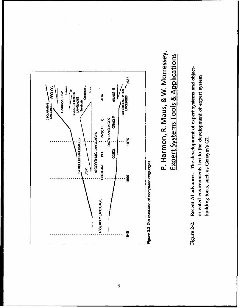
The evolution of computer languages is illustrated in Figure 2-1. Assemblylanguage was dominant between World War !I and 1960. In the late 1950s, higher
order languages (HOLs) began to emerge. FORTRAN was one of the first HOLs andwas developed as a scientific programming language.
In the early 1960s programming languages began to take two paths: symboliclanguages and algorithmic languages. Symbolic languages are oriented moretowards logic and list (eg: text) processing than numerical processing. One of thefirst and most common symbolic languages was LISP. A number of algorithmiclanguages were also developed between 1960 and 1985 including FORTRAN, PL1,PASCAL, C and ADA.
Computer languages began to branch out again in the early 1980s. Symboliclanguages began to expand into PROLOG, LISP, and Object-Oriented approaches.Meanwhile, algorithmic languages began to incorporate symbolic language features.For example, C++ is an extension of C, based on object-oriented programming.Also during this time, so-called "Fourth Generation" languages began to emerge.Fourth Generation languages again raised the level of abstraction and are
commonly associated with database management systems. By 1985 the programmerhad a host of languages available in a number of varied approaches.
The emergence of Expert Systems and object-oriented environments led to
the development of Expert System Building Tools, such as Gensym's G2. This isillustrated in Figure 2-2. Also note in Figure 2-2 that academic research into
7

OAC,
A.A 0cu -
CC
S0
uh 0 >~
rz. I -1w W
x U(
'.o
.... . .. .... .... .... .... ...
I-.
I.- .
n IL
U 4w
0I0
E o-____ ____ ___ ____ ___ ____ ____ ___ ____ S>
9C

Artificial Intelligence (AI) is leading and feeding practical Al developments inbusiness, industry, and government. Today, some of the leading Al activities are inthe areas of distributed processing and Very Large Expert Systems, which includesdevelopments in "Blackboard" technologies.
Is the Object-Oriented approach "better" than other approaches? Notnecessarily. However, the object-oriented approach is appealing for a number ofproblems, including the ES CFAR system. A key point being made here is that,
S~unlike 1960, the programmer today has a variety of approaches available. Theapplications programmer' (eg: signal processing algorithm developer) needs to beaware of these advances in Al in order to fully exploit the new computertechnologies.
One goal of this report is to describe the specific expert system tool being usedto build the ES CFAR application. This discussion begins with a general descriptionof how expert systems work, describing their components and how the components
interact.
2.1.1 Expert Systems
An expert system can be described as a computer based system that usesreasoning techniques to automatically search, analyze, and exploit knowledge thathas been appropriately represented within the computer. With conventionalcomputing techniques, reasoning based search and analysis tasks must be performedin the minds of the human expert. The success of expert systems depends on theirability 1.) to store or represent as a computer knowledge base the domainknowledge, associated with "human expertise", in a manner that enables logicalinference ("the knowledge representation problem") and 2.) to search, withinreasonable time constraints, through this knowledge base for solutions tointeractively posed "domain" problems ("the search problem"). While expertsystem designs can vary, they all tend to have a knowledge base, an inference
engine, and an interactive user interface.
10
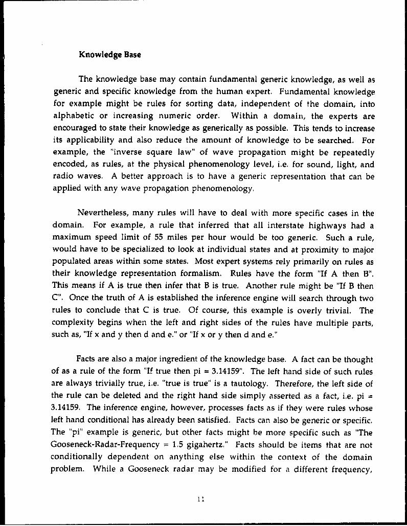
Knowledge Base
The knowledge base may contain fundamental generic knowledge, as well asgeneric and specific knowledge from the human expert. Fundamental knowledgefor example might be rules for sorting data, independent of the domain, intoalphabetic or increasing numeric order. Within a domain, the experts areencouraged to state their knowledge as generically as possible. This tends to increaseits applicability and also reduce the amount of knowledge to be searched. Forexample, the "inverse square law" of wave propagation might be repeatedlyencoded, as rules, at the physical phenomenology level, i.e. for sound, light, andradio waves. A better approach is to have a generic representation that can beapplied with any wave propagation phenomenology.
Nevertheless, many rules will have to deal with more specific cases in thedomain. For example, a rule that inferred that all interstate highways had amaximum speed limit of 55 miles per hour would be too generic. Such a rule,would have to be specialized to look at individual states and at proximity to majorpopulated areas within some states. Most expert systems rely primarily on rules astheir knowledge representation formalism. Rules have the form "If A then B".This means if A is true then infer that B is true. Another rule might be "If B thenC". Once the truth of A is established the inference engine will search through tworules to conclude that C is true. Of course, this example is overly trivial. Thecomplexity begins when the left and right sides of the rules have multiple parts,such as, "If x and y then d and e." or "If x or y then d and e."
Facts are also a major ingredient of the knowledge base. A fact can be thoughtof as a rule of the form "If true then pi = 3.14159". The left hand side of such rulesare always trivially true, i.e. "true is true" is a tautology. Therefore, the left side ofthe rule can be deleted and the right hand side simply asserted as a fact, i.e. pi =
3.14159. The inference engine, however, processes facts as if they were rules whoseleft hand conditional has already been satisfied. Facts can also be generic or specific.The "pi" example is generic, but other facts might be more specific such as "TheGooseneck-Radar-Frequency = 1.5 gigahertz." Facts should be items that are notconditionally dependent on anything else within the context of the domainproblem. While a Gooseneck radar may be modified for a different frequency,
Ii

within the context of the current problem it will not be so modified Obviously,some facts are more secure than others. The value of "pi" is a safer fact, then theassertion of a system's radio frequency.
Inference Engine
As already implied, the inference engine is an algorithm that concludes newtruths from known truths. The process is deductive inference in that the results arealways correct. Inductive and abductive inference by contrast can only suggestsolutions that may be true, i.e. hypotheses.
When the inference engine proceeds, as in the above example (from the truthof A, to the truth of B, and finally to the truth of C), this is called "forwardchaining". In this case, each rule is applied from left to right. The rules can also beapplied in the reverse direction which is called "backward chaining".
Most expert systems use backward chaining because they are goal driven, i.e.given that the desired solution is C, how can the system find a path to C. In thiscase, the rule "if B then C" would be applied first with the conclusion that a waymust be found to show that B is true. Next, "if A then B" will be applied because theright hand side matches with the B goal. Now, given that A is a "fact", the search is
complete. However, as mentioned above, the inference engine actually treats thefact "A" as a rule, i.e. "if true then A." Thus, the inference engine actually backwardchains one more step, matching the left hand side of "if A then B" with the righthand side of "if true then A." The inference engine therefore responds with "true",meaning that the goal state C is true.
For most problems, backward chaining seems to result in more efficient,meaning faster, searches by the inference engine. The desirability of forward versusbackward chaining depends on the forward and backward branching factors for therules. This relates to how many "and/or" components exist in the left and right side
of the average rule. The trick is to use the direction that generates the smallerexpansion of possible search paths. While most expert systems perform better with
backward chaining, expert systems for manufacturing control and other planningproblems, tend to perform better with forward chaining. This is because they areconstrained by their starting conditions but can accept multiple solutions or end
12
conditions. A backward chaining scheme corresponds to a constrained goal withmultiple acceptable starting conditions.
Interactive User Interface
An expert system normally has two types of interactive users: the domain
expert and a non-expert user of the domain knowledge. Through the interactiveinterface, which is often a graphical user interface with easy-to-use "pull down"menus, the expert can insert, critique, and modify the domain knowledge of thesystem. The non-expert user can insert problems and receive solutions, along witha rationale or logical explanation. The logical explanations are actually theknowledge inserted by the domain expert. In this way, the user can go to the systemfor consultative support rather than going to the expert. In this sense, the systembecomes a productivity multiplier for the human expert. The explanation capabilityis a key aspect of expert systems technology. The system is not only supposed toprovide a solution, it is supposed to convince the user that the solution is correct.
Expert System Development Shell
Since the shell provides all of the deductive reasoning algorithms for theinference engine, the system developer can concentrate or focus on the specificationof declarative domain knowledge for the knowledge base, rather than on thedevelopment of search strategies.
Key to the development of an expert system is the description of theknowledge an expert uses to solve a problem. There are a number of ways torepresent this knowledge in a knowledge base. While rules are the easiest to
understand from a deductive inference viewpoint, knowledge can also berepresented as frames, semantic networks, scripts, relations, or even procedures.
Various expert system environments support many of these alternatives, in
addition to rules. Some of these formalisms, however, while adding run-timeefficiency and even ease of knowledge capture are not amenable to automatedinference. In particular, a procedural representation can not be checked by theinference engine for internal consistency--an illogical programming step ("bug")
will normally not be detected by the inference engine as it might be in a rule basedformalism. Nevertheless, procedures are pragmatically necessary.
13

The extension of knowledge representation techniques, beyond the ruleformalism, is nicely facilitated by object oriented programming (OOP) methods.Object oriented systems provide a simple, natural way of capturing relations whichcan be used to represent rules, semantic nets, and other formalisms. In objectoriented programming, the programmer defines classes of objects for an application.Each class definition includes a programmer-provided list of attributes. Objects canthen be dynamically created as instances of the class. Each instantiated object canhave different values assigned to the attributes. The classes can and should exist
within a class hierarchy to facilitate inheritance. All attributes should be defined atthe highest possible class level in the hierarchy. This means they should be asgeneric as possible. Each lower level class inherits the attributes of its superiorparent , but it can also contain its own, more specific, attributes. While classes andclass hierarchy structures are defined solely by the developer, as a rule of thumb,most classes are defined in ways that strongly parallel their existence in the real
world. Thus, the program successfully models the real world relationships.
Using the object oriented approach gives the developer the ability to structureand easily define a large number of facts and relationships without having toincorporate them as rules. Rules can be reserved for those cases where they are themore natural representational form, i.e. when the heuristic knowledge in thedomain has a natural "if.... then ..." rule format. Such heuristics, while often basedon incomplete evidence, can easily capture a human expert's "rule-of-thumb"
intuition about the domain knowledge.
Inference and Control
Expert system programming involves finding the appropriate description ofdomain knowledge so that it can be represented declaratively, rather thanprocedurally within the system. This means that minimal programming is requiredto utilize the knowledge; the inference engine provides the programmatic logic.The control and search strategies that the inference engines employ are pre-
developed and are not typically governed by the developer. In this way, the sameinferencing techniques can be applied for the control of many kinds of knowledge
bases and applications.
14

Inference engines are typically described by the types of inference and controlstrategies that they employ. One or more inference engine control strategies may beavailable in a particular expert system environment. The most common techniquesare forward and backward chaining, described above, and breadth first versus depthfirst search.
The latter option addresses how the system will cope with branching factors ateach level of rule application in the inference cycle. Breadth first means that all ruleoptions are generated at each level before proceeding to the next level. Depth firstmeans that only one rule is applied at each level before proceeding to the next level.Depth first will on average find a solution in half the search time of breadth firstsearch. However, depth first must know a priori how many levels exist. If it stopsone level short of a solution it won't find it. When depth first reaches the lowestlevel without finding a solution, it backs up one level and tries the next matching,but not yet tried, rule. It then proceeds down again in a depth first mode.Eventually, the system, by backing up and going forward again, will exhaust theavailable rules at all levels. i.e. That is, if it backs up and there are no more untriedrules at that level, it backs up again, eventually reaching the top before proceeding
down again. While breadth first takes twice as long on average, it does not have toknow in advance how many layers to try. It exhausts all rule applications at eachlayer before proceeding to the next layer.
Other control strategies are also available such as heuristic search wheremeta-rules are used to prune unlikely, though legal inferences, from theexponentially expanding search tree. Rules can also be grouped into hierarchicallyrelated sets so that at different levels in the tree, the number of rules that have to belinearly checked for a match is reduced. Hashing and other specialized patternmatching techniques can be used to increase the efficiency of the search process.
Some techniques are more closely associated with formal logic, specifically firstorder logic or predicate calculus. This set of techniques is now generally known aslogic programming. The inference step for this formalism is known as resolution
and the binding from rule to rule in this inference process is controlled byunification. A popular system for logic programming is Prolog whose resolutionbased inference is equivalent to a backward chaining, depth first search.
15

In summary, inference systems can be thought of as deductive, inductive, orabductive:
0 Deductive systems apply rules to derive absolute, but non-explicit,hidden truths from explicitly known truths.
0 Inductive systems try to find rules by searching for correlationsbetween factual events over a large sample size. This process, unlike deduction, isnot fail safe. Correlating sunlight with growth can correctly lead to the rule that "ifthe sun shines then the plants grow." However, other, seemingly plausiblecorrelations, can lead to illogical rules such as "If the sun passes over head once aday then it circles the earth once a day."
* Abduction generally applies known rules in a backward chaininghypothetical sense. It can not prove the truth of an earlier event, but only thepossibility that something might have occurred which caused the later event to betrue.
Expert systems have been built that address all three of these inference types.Induction and abduction usually require a second level of abstraction in theinference engine. Most expert systems, and virtually all applied expert systems, arerestricted to deductive logic. While the programmer and the domain expert maypractice inductive inference to find the rules, this is normally a human rather than
a machine inference process. The machine restricts itself to the deductiveapplication of the given rules. It may, however, challenge the validity of thehuman inductive mechanism's results when two rules are found to be mutuallyinconsistent, but applied systems do not normally infer their own rules. Inductivelyinferring rules is actually a form of machine learning; it is currently an active and
exciting research area.
In addition to the variability of inference mechanisms, knowledgerepresentation techniques can also vary from a strict compliance with the rule-basedformalism to the incorporation of frames, scripts, semantic networks, and otherrelational strategies. Hybrid systems are rapidly evolving that allow the advantagesof a rule based deductive inference formalism to be combined with other advancedrepresentational strategies as well as with conventional programming techniques.
16

Object oriented environments provided the necessary structure for 3uchhybrid systems. In these systems, a core module can provide the rule-basedinferential control, while allowing the lower level processes, such as conventionaldigital signal processing, to remain as sub-routines in conventional procedure basedlanguages. This facilitated by the fact that procedures and rules can all be thought ofas objects and thus easily integrated by the object oriented environment.
2.1.2 G
Gensym's G2 is an expert system tool which is being used to prototype anddevelop the ES CFAR expert system. It is a complex system which uses the power ofobject-oriented programming with a hybrid inference engine and the use of bothrules and procedures in order to offer one of the most flexible environments
possible for systems-development. Application development is doue in a graphical,object-oriented environment with support tools which provide for both rapidprototyping and full scale system development. Gensym's G2 was selected forprototype development because of its professional-level capabilities, graphical userinterface and development environment, and its availability of support.
The first step in developing an application with G2 is defining the class ofeach object in the application's knowledge domain. In the ES CFAR application, thekey class definitions include radars, clutter, targets, CFAR-processes, and detections.Along with defining the object classes and their attributes, one must also define the
class hierarchy.
The class hierarchy identifies how certain objects are related to others and
how objects inherit attributes from their superior classes. Consider, for example, theclass of objects named clutter. The class clutter (within the ES CFAR application)
has an attribute which defines whether .he clutter is Weibull, exponential, log-normal, etc. Each of these specific subclasses of clutter have attributes that aredescriptive of their "statistical distribution" such as mean and variance. Eachsubclass also inherits the attributes of its superior class. Another example from theES CFAR application which describes how class definitions identify relationshipsbetween objects can be seen in how the class of radar objects is defined. A radar has
subsystems and characteristics defined as attributes of the radar: antenna, receiver,
17

transmitter, beam, and direction. Each of these subsystems is itself a unique class ofobjects with unique attributes that describe each specific subsystem. By defining eachsubsystem class as an attribute of the class "radar", each instance of a radar includesan instance of each the subsystems.
Once the developer has defined the class hierarchy and all classes, a model ofthe application is created. The model includes all relationships, objects, rules, and
procedures that describe the application. The developer organizes this knowledge inthe knowledge base by placing related items on a single workspace. Workspaces arethe places in the knowledge base where the items which make up the knowledgebase are located. The workspaces are also structured in a hierarchy ofsubworkspaces. One way the developer may organize the items in the knowledgebase is to have a superior workspace as a menu with selections such as rules, objectdefinitions, procedures, user-menu-choices, etc. Each of the selection objects on themenu have a subworkspace, where a collection of like objects are collocated.
The workspaces, objects, rules, procedures, etc., make up the knowledge base.All this knowledge describes how the attributes of the objects are related and how
they can receive their values.
G2 offers sources which determine how attributes can uniquely receive theirvalues. Attributes can receive their values from the inference engine, the G2
simulator, through "real-world" sensors, and through the G2 Standard Interface(GSI). The inference engine uses its inferencing mechanism to determine thevalues of attributes. The G2 simulator produces values through the use ofsimulation formulas. When attributes receive true values through "real-world"sensors, the GSI is used to connect the G2 variables with external sensors. The GSI is
also used to connect G2 with external data sources such as with remote processes. Inthe ES CFAR application, the remote procedure call (RPC) is used frequently toobtain values for variables (through the GSI) from remote C-programs. In the ESCFAR application, some of the key processes are numerically intense and need to beexecuted in a remote environment. For instance, the radar data is processed by a
CFAR algorithm in order to report detections. In this case, G2 determines whichCFAR process should be used to process the data and sends this information
through an RPC to the CFAR process which is coded in C language. The CFAR
process or outputs detections, which are sent back to G2 through another RPC.
18

In the ES CFAR application, as well as in a wide variety of other applications,the best solution for a problem results from a combination of symbolic andprocedural programming. Knowledge engineers must analyze the problems anddecide how to distribute them between procedural code (either in G2 or remoteprocedures) and expert system techniques. In the ES CFAR system the use of remote
procedures in the form of C code results in a faster system as well as the ability to usestatistical routines not provided in the expert system development shell (G2).
2.2 KBS Overview
A variety of diagrams have been developed to design and illustrate the ES
CFAR system since both procedural and symbolic aspects need to be represented.Figure 1-1 showed an overall schematic of the current ES CFAR system that
emphasizes data flow and data displays. Beginning at the upper left of Figure 1-1,radar data flows to the baseline CFAR and ES CFAR processes. The baseline CFARpath represents conventional CFAR processing and is indicated by everything abovethe horizontal dashed line. The radar data may be either simulated or measured. Adisplay of received power versus range is available by "clicking" on the POWER-VERSUS-RANGE icon. The baseline process exercises a user selected CFARalgorithm on the same data as the ES CFAR process for comparison purposes. Theoutput of the baseline process is a list of detections, which can be displayed in PPI
format ("click" on BASELINE-CFAR-PPI) and which flows to the performancemonitoring process for calculation of actual Pd and Pf. The CFAR-PROCESSING-PERFORMANCE icon brings up a comparison display of time histories of Pf and Pdfor the baseline and ES CFAR processes.
The radar data also flows into the ES CFAR process. Prior to actual ES CFAR
processing, the radar data flows to a series of processing routines (the pre-processor)that find discretes, classify the radial of data into relatively homogeneous clutterregions, and integrate additional sources of information such as geographic data,radar position information, user input and knowledge about the target. Thisinformation is used to select the CFAR algorithm(s) to be used for the variousclutter regions. A list of clutter regions and the associated CFAR algorithms thenflows to the ES CFAR process. The ES CFAR process exercises the CFAR algorithmson the radial of data and produces a list of detections. Currently, Cell Averaging,
19

Greatest-Of, Trimmed Mean, and Ordered Statistics CFAR algorithms are beingimplemented. The WEIGHTING AND FUSING and FALSE ALARM CONTROL
processes will then operate on this list of detections to produce the final list of ESCFAR detections. These two processes have not yet been implemented. The list ofdetections flows to the PERFORMANCE MONITORING circuit so the actual Pf andPd for the ES CFAR process can be computed and displayed. As with the baselineprocess, a PPI display of detections is available from the AI-CFAR-PPI icon and thetime history of Pf and Pd is available from the CFAR-PERFORMANCE-MONITORING icon. The TRACKER process will operate on the list of detectionsand maintain a target track, when it is fully implemented.
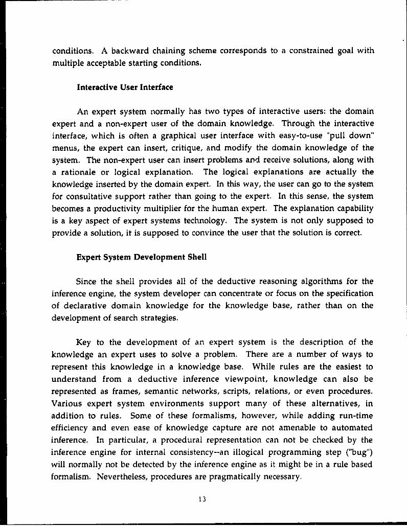
While the basic data flow through the ES CFAR system can be seen in Figure1-1, another diagram is needed to show where these processes are implemented andhow the data is transferred between them. Figure 2-3 presents this kind ofinformation. As noted earlier, several software tools are being used in the ES CFAR
system. The user interface, process control, and inferencing are performed by G2and include the following items in Figure 2-3:
"* Overall Process Control
"* Radar Parameter User Interface"* CFAR Parameter User Interface"* Data Weighting
"* CFAR Selection"* Detection - Weighting-a nd-Fusing"* False-Alarm Control
"* Performance Monitor"I Pd - Pf - Statistics
Computationally intensive processes are implemented using remoteprocedures, called through GSI. These remote procedures are being developed in C
and include the following functions in Figure 2-3:
"* Radar Data Generator"* Statistical Distribution Identifier"* Clutter Classifier". Baseline CFAR Process
20
DATA TRANSFER SCHEMATIC
START- RAD IAL-P ROCESS
OVEAL-PRCES-CNTOLTARGET-DATA 7ARGET-UI
CLLUETCLSSRIE LIST-OF-CLUT-REGION
TARGET-TRCK-RPANFOER RAA-EI DIL-AOF-FUSE
FINAL-DETECTIONUlSTPD-PFASTAT AC IETIAFIER PF
FiUrER2-3:F Dat Trasf Sceatc The- KigrmshWLErDGrouEpoese
are mplmentd ad hw daa i trasfered
21T-F--
* ES CFAR Process* Tracker
Processes that need a quality graphical display capability are implementedusing a commercial graphics package called PV-WAVE. These processes include:
* Target User Interface* Clutter Map User Interface* Radar Data Plot• PPI Plot
The remaining items include various data transfer items needed for inter-
process communication.
Examples of G2 subworkspaces are shown in Figures 2-4 through 2-7. Theuser begins the simulation from the G2 main menu by selecting "Get Workspace"and then selecting the "Welcome" workspace, shown in the upper left panel ofFigure 2-4. Desired subworkspaces then appear automatically or are user selectable
as the user sets up the simulation. The source for the radar can be selected (i.e.,simulated or real), although the "actual I-Q data" selection has not yet beenimplemented. Figure 2-5 shows the subworkspaces and menus for setting up theradar. Predefined radars can be selected and radar parameters can be modifiedthrough the radar subsystems tables. Next the CFAR selection menu appears as
shown in Figure 2-6. One CFAR algorithm can be chosen for the baseline CFAR.Any or all of the CFAR's can be chosen as candidates for the ES CFAR selectionrules. Currently, simple rules only for testing purposes are being used (e.g., always
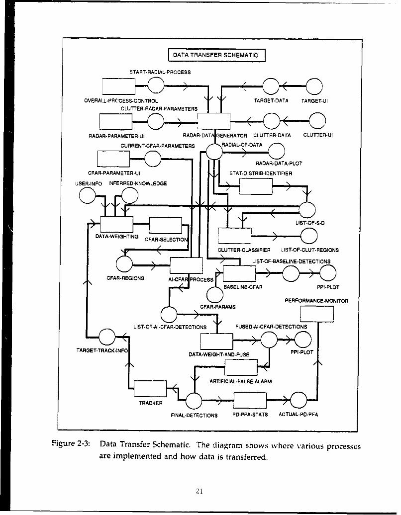
choose OS). Next the subworkspace of "Simulation Map" appears as shown inFigure 2-7. The user can place targets on the map and change clutter attributes byclicking on the CFAR-TESTING-CONTROL button. The actual simulation beginswhen the "Simulation On" button is selected.
G2 begins the radar simulation process by calling the appropriate remoteprocedures. As the user defines the simulation via menus in G2, data is sent to the
remote procedures and is stored in global variables. For example, when the radarhas been defined by selecting a predefined radar and perhaps changing some of itsparameters (as shown in Figure 2-5), the information is passed to the remote
2 '2

* -diE~I - .4-
__ UJt.
V, -C SM
LU)
U)U Q
rz-1 I- c)
0~ .2w cu X C-4
_ _ _ _ LU*4
#A E
2LE
U.~0 E)'2- 00) 4)
w >i
o U)
IL ~' U 23

=1~Ln
F 1swIil I, I
I] L
z U41111 1l _cr. C LL~0 Z
cc w U* Q *z AEi11 ILcuU)icu 6
211~
24

i5"
o-LLrr(~ LL
22 -G
CC
.0
CL ".0
C L<L _co)
000
0) U) < 0<LLC
25
......~TrT ..... .. .OO C ~ I ......... ..L.- -1J ,W I
"0101% INNN
M .........VS T.S
~ jzzj0CR AT~ATA
E 0 .
..1W ~ ........ .....
Xzz: ::i*iLR.
Tan eae I atre
Noe:XRE-XX3:O
Use .et..ton none... Name......Ti.
... o...117
Ypos-16
Rag 613.3
Aziut 106.5....8
Figure~~~~~~~~~~~~~ ~. 2-:Sbwr.ac.o.onrlin.h.imlton.uter .borsae
are acesbeb cikn'o h aiu it utn..The.table.a
lowerabl rightr show a targetsatrbe.
Noe26RE-XX3:O

procedures by calling the remote procedure SEND-RADAR-PARAMS, which storesthe information in a global data structure. The radar parameters are thus madeavailable to the other remote procedures. The user can select clutter regions and setvarious attributes of the clutter, such as statistical distribution, backscattercoefficient, and distribution shape parameters from the "Simulation Map"subworkspace shown in Figure 2-7. The clutter region information is passed to theremote procedures by calling SEND-CLUTTER-PARAMS for each of the clutterregions. The clutter regions are stored in a linked-list structure. Similarly, the usercan create targets and place them relative to the radar location. The list of targets issent to the remote procedures where it is stored as a linked list. The target attributesthat are currently passed are range, azimuth, and radar cross section, as shown in thelower right panel of Figure 2-7.
Workspaces contain logically related objects. It is convenient for the user ofthe ES CFAR system to also provide documentation on the workspace. Adocumentation tool, shown in Figure 2-8, was written to help the KB developerdocument items on the workspace. A sample of documentation on a subworkspaceis shown in Figure 2-9.
2.3 Simulated Data
The current set of remote procedures contains functions to generate
statistically independent random variates with exponential, Weibull, and log-normal distributions. During the course of the ES CFAR system development,many tests have been run to verify the correct performance of the functions in theremote procedures. The gen raddata function generates received power data andstores it in an array for subsequent processing. The data is currently stored in a discfile for interfacing to PV-WAVE for plotting. (With the new version of PV-WAVE,this disc file will be eliminated because disc access is relatively slow for inter-processcommunication.) Figure 2-10 shows received power versus range for a noise-onlyenvironment. The data follows an exponential distribution. Figure 2-11 shows thecorresponding received power histogram for the noise-only radial, with amplitudeconverted to dB. A radial of data with a segment of Weibull-distributed clutteradded to the noise is shown in Figure 2-12. The clutter extends from range cell 333through range cell 665 with a backscatter coefficient of 10-7. A received powerhistogram of this data is shown in Figure 2-13. In addition to clutter, gen_rad_data
27

CDU
a)
0 ®.o 'a
CL 4-
E a)4>. -)o
/o • o
0 E•
aCU
0 0
0-0 0)
,•,,
0 CD
2 0
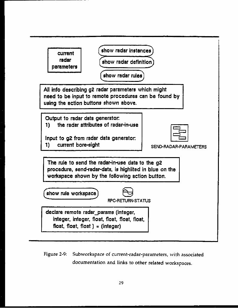
current show radar instances
radar (show radar definition)parameters
cho! rdar rules•
All info describing g2 radar parameters which mightneed to be input to remote procedures can be found byusing the action buttons shown above.
Output to radar data generator.1) the radar attributes of radar-in-use
Input to g2 from radar data generator.1) current bore-sight SEND-RADAR-PARAMETERS
The rule to send the radar-in-use data to the g2procedure, send-radar-data, is highlited in blue on theworkspace shown by the following action button.
(show rule workspace)'
RPC-RETURN-STATUS
declare remote radarýparams (integer,integer, integer, float, float, float, float,float, float, float) = (integer)
Figure 2-9: Subworkspace of current-radar-parameters, with associated
documentation and links to other related workspaces.
29

Racial Data Plot
' -120,140
gL;
0 200 400 600 S00 1000Racial Cell Number
Figure 2-10: Representative noise-only radial of radar received power.
Histogram of recewveC o.wer100"i
80-
LF
60
40-
20-
0 20 40Received Power (dB), relotive to -165.616
Figure 2-11: Histogram of received power in noise-only radial.
30

Radial Octo Plot
-120 2
-So
I.1
0 2CN 400 600 800 00CRadial Cell Numoer
Figure 2-12: Radial of received power including noise and a segment of Weibull
clutter. The clutter extends from range cell 333 to range cell 665.
Histooram of -eceivea oower
S60"
0 40
20
0 20 40 60 80 10
Received Power (dB), rilotive to -170.527
Figure 2-13: Histogram of radial con aining noise and a Weibull clutter segment.
31

can add targets and discretes. This is illustrated in Figure 2-14. The largest return inFigure 2-14, at range cell 400, is the target. Additional high values of received power
are mainly discretes, which have been added every 20 km. Figure 2-15 shows thehistogram of the radial with noise, clutter, discretes and a target included.
A number of statistics are computed on the clutter segments. These statistics
are sent from the remote procedures to G2 by a call to send-clutter-regions. It isanticipated that these statistics will be used in selecting the CFAR algorithm for agiven clutter region. Figure 2-16 shows G2 tables of statistics for two clutter
segments. The statistics are the mean, median, minimum, maximum, standarddeviation, skewness, kurtosis, and the autocorrelation at lags (delays) 1, 2 and 3.
2.4 Implementation of CFAR Algorithms
Four CFAR algorithms have been selected for use in the ES CFAR knowledgebase: Cell averaging (CA), greatest of (GO), ordered statistics (OS), and trimmedmean (TM). These algorithms were coded in C, using the description in Gandhi
and Kassam [1]. The C functions are designed to operate on a sliding window, withthe test cell at some location within the sliding window. For the baselineimplementation, the calling function moves the sliding window through the radialof data, with the test cell centered in the window. Tests are not performed for thefirst n/2 range cells or the last n/2 range cells, where n is the number of values used
for the sliding window, since a full window is not available for averaging in those
cases.
In the AI implementation, the radial is divided into segments of relativelyhomogeneous clutter, based on the clutter edges. The ES CFAR module receives alist of segments from G2 and then exercises the appropriate CFAR algorithm in a
given clutter segment. Since the radial is divided into multiple segments, the
baseline method of applying the sliding window would result in excessive gaps inrange cell processing at the transition regions between segments. Therefore, a
different sliding window method is used for the ES CFAR. In the ES CFARfunction, the first range cell is also the first test cell. The sliding window is
composed of n range cells at farther ranges as shown in Figure 2-17 (a). The windowremains fixed while the test cell advances until the test cell is centered in the
window. The window and test cell then advance together, keeping the test cell
32

-601 Z-.aioI :oto Plot
-80L
,, -1207
xv- -40
.- 160 i
-180' I
0 200 400 F00 800 1000Radiat Cell Number
Figure 2-14: Received power for a radial containing noise, clutter, a target, anddiscretes. The target is located at range cell 400. Discretes are locatedevery 20 range cells.
Histoorom of received power80°I
760
S40UIl
'I- *120ý
0 ~0 20 40 60 80 100
Received Power '48), relative to -171.321
Figure 2-15: Histogram of radial containing noise, clutter, a target, and discretes.
33
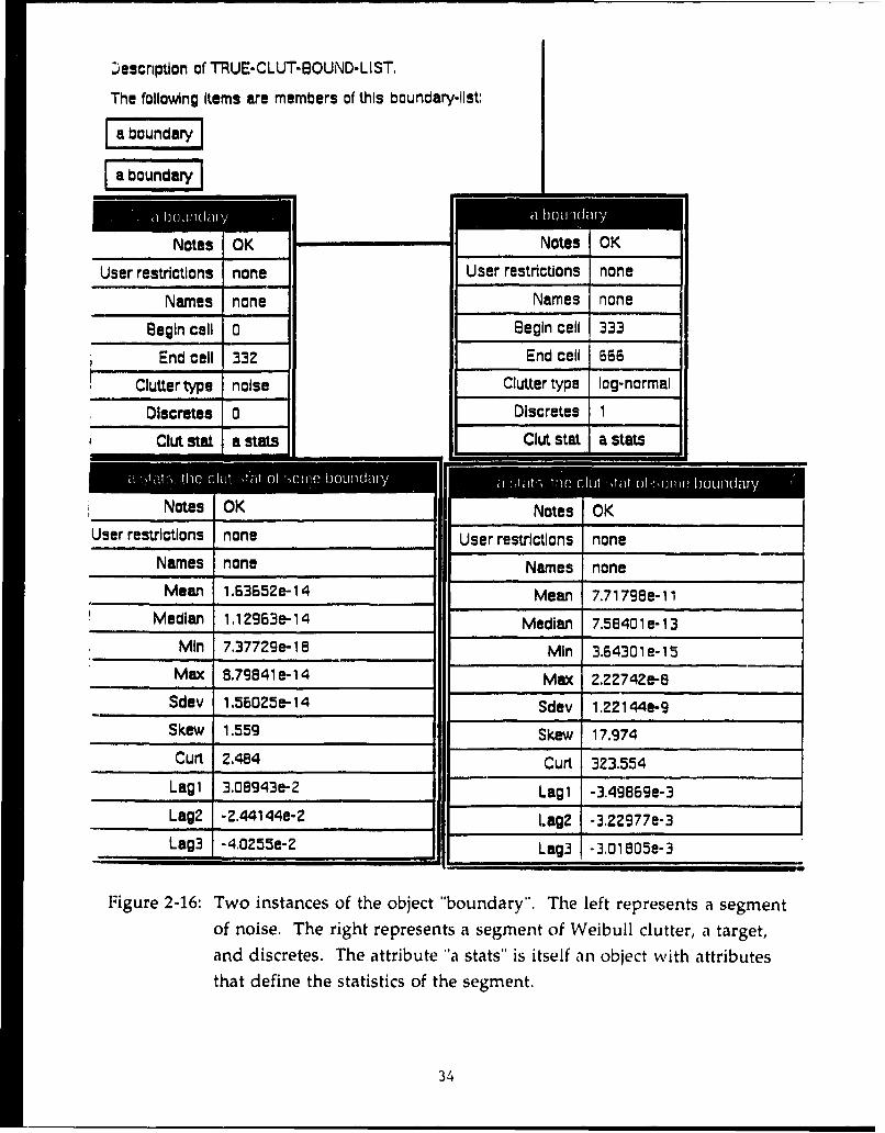
Description of TRUE-CLUT-83OUND-LIST.
The following Items are members of this boundary-list:
dary
User restrictions none User restrictions none
Names none Names none
Begin cell 0 Begin cell 333End cell 332 End cell 666
Clutter type noise Clutter type log-normal
* Dlscretes 0 Discretes 1
Clut stat a stats Clut stat a stats
*Notes OK Notes OKUser restrictio~ns none User restrictions none
Names none Names noneMean 1 .63652e- 14 Mean, 7.71798e- 11
Median 1.12963e-14 Median 7.58401ea-13Min 7.3772ge- 18 Min 3.64301a- 15
Max 13.791941 e-14 Max 2.22742e-8
Sdev 1.56025e- 14 Sdev 1,22144e-9Skew__1__55_ Skew 17.974
Curt__Z.484_ Curt 323.554
_____3.08943e-2 Lagi -3,4986ge-3
Lag2 2.4414e-2Lag2 -3,22977e-3
Lag -4025e-2Lag3 -3.01805e-3
Figure 2-16: Two instances of the object "boundary". The left represents a segmentof noise. The right represents a segment of Weibull clutter, a target,and discretes. The attribute "a stats" is itself an object with attributesthat define the statistics of the segment.
34

test cell
Di - D D ,I D0 e Dn
Target
CFAR PROCESSOR I-No targetT'
E' (Dn) r
C (Pfa,nf)
Figure 2-17 (a): Sliding window and test cell for processing the first cell in a
clutter segment (expert system path).
test cell
D, -00 D D2 D3 .. Dn
-•Target
CFAR PROCESSOR - -No targetT'
C( Pfa,n)
Figure 2-17 (b): Sliding window and test cell for processing the second cell in aclutter segriient (expert system path).
I i I l I51 l

centered, until the leading edge of the window reaches the end of the processingsegment. At that point the window remains fixed while the test cell advancesthrough the window. The various test cell and window states are illustrated inFigure 2-17 (a-e).
When the first processing segment within the radial is completed, thewindow is positioned at the start of the next segment with the test cell designated as
the first range cell of the new segment. Processing continues as before until allsegments in the radial have been processed.
Implementation of the CA and GO algorithms is straightforward. Processingis mainly the accumulation of sums. However, for the OS and TM algorithms thedata needs to be sorted and then either a value is picked (OS) or the smallest andlargest values are censored (TM). Sorting is accomplished by a heap sort [2] of the
pointers to range cells in the radial of data. The data in the radial is thereforeundisturbed for processing adjacent test cells.
In making detection decisions, a threshold multiplier is needed forcalculation of the threshold from the appropriate test statistic from the data. Thethreshold multipliers are computed based on the Gaussian assumption as in Gandhiand Kassam [1]. These equations are solved by bisection numerical techniques in aseparate program for several values of Pf and the values are inserted in the
functions that implement the sliding window. The solution of these equations willbe added to the remote procedures of the ES CFAR system and provide thresholdmultipliers that can be updated for any radial.
2.5 Performance Measures
The performance measures implemented in the current ES CFAR system arethe actual Pf and Id for the baseline and ES CFAR processes. Since the targetlocations are known for the simulated data, the list of detections can be divided intotrue detections and false alarms. These numbers are accumulated along with thenumber of test cells and the actual Pf and Pd are computed as:
P= (number of false alarms)/(number of test cells without targets)Pd = (number of true detections)/(number of actual targets)
36

test ceill
Di -- *I DI D2 0 Dn/2 Dn/2 + I Dn-1 ni
000 @000
CFAR PROCESSOR -- No target
C( Pfan)
Figure 2-17 (c): Sliding window and test cell when the test cell is far from a
clutter boundary (expert system path).
'3 7

test cell
Di ---* I 0D2 In DI. D Dn
ego_ Target
CFAR PROCESSOR !No target
C( Pfa,n)
Figure 2-17 (d): Sliding window and test cell for the second to the last test cell ina clutter segment (expert system path).
test cell
Di -111 D I D2 •* Dn D
S *•nTarget
CFAR PROCESSOR No targetL T'
C (Pfa,n)
Figure 2-17 (e): Sliding window and test cell for the last test cell in a cluttersegment (expert system path).
38
The Pf and Pd for both the baseline and ES CFAR processes are sent to G2
using GSI, the G2 Standard Interface. GSI is used to build interfaces between G2 and
external applications. Currently, the display of Pf and Id on the time history plot
causes data-seeking for values of Pf and Pd. That is, when the display realizes it
needs a value for the variable Pf or Pd, it searches for it. Sample time histories of Pf
and Pd are shown in section 2.6.
2.6 Testing and Verification of CFAR Algorithms
Several different tests were performed on the CFAR algorithms during their
development and integration into the ES CFAR system. The CFAR algorithms were
developed on a 486 computer using Borland C++. A 486 was used so that the SUN
SparcStation could be used for other work that required its graphical capabilities.
While a CFAR algorithm was being developed, a test program was used to generate
a radial of exponentially distributed clutter to exercise the CFAR algorithm. The testroutine computed an actual Pf, which could be compared to the value used to set the
threshold for the CFAR routine (ie: the design Pf). When a CFAR routine passed
this test, it was then ported to the Sun SparcStation.
To assure that the CFAR routines were correctly incorporated into the ES
CFAR system, several test runs were performed. A test case was constructed by
inserting a Swerling I target of known radar cross section at a specified range. The
test was constructed in this manner to perform a sensitive test of CFAR function
logic, threshold calculations, and the distribution of the simulated radar data. To
construct the test case, the "AK" radar, which is one of the representative radarsincluded in the ES CFAR system, was selected. For a known SNR, the Pd for a
Swerling I target can be computed for exponential clutter or noise using the
equations found in Gandhi and Kassam. A SNR of 10 dB was selected since it
provides a Pd of approximately 0.5. For the "AK" radar parameters, a target with a
radar cross section of -20 dBsm at 74.87 km will give a 10 dB SNR, using the standard
radar equation.
To test the CFAR routines in. the ES CFAR system, additional rules were
added to the knowiedge base to conveniently set up the test. These rules generate
targets with a user selected RCS and insert them in the list of targets at azimuths
39
that are one beamwidth apart. This setup gives a sufficiently large number of actualtargets within a reasonable amount of run time to compute actual Pd. In setting upthe test cases, the Pf is set to a rather large value, 0.001, so that many false alarmsoccur for calculation of actual Pf. In addition, the four CFAR algorithms were tested
separately , so rules were added to select only a predetermined CFAR for the ESCFAR path. The same CFAR algorithm was selected for both the baseline and ESCFAR paths. The ES CFAR system was then run long enough to generate at least
300 detected targets.
One of the workspaces in the ES CFAR system allows the user to monitoractual Pf and Pd. The GSI returns values of actual Pf and Pd for both the baseline
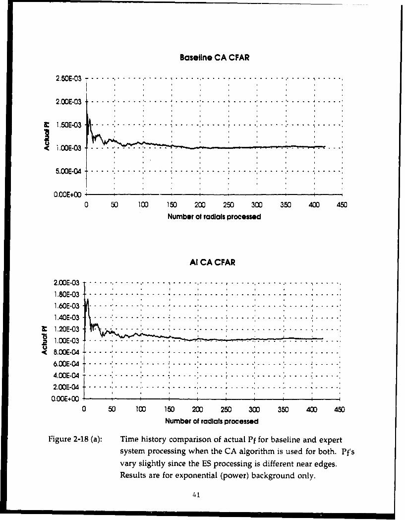
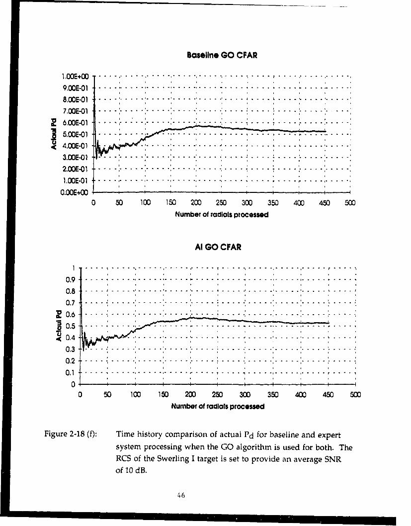
and the ES CFAR paths. The history-keeping attribute is set so that the previous 200values can be shown on a graph. Time history performance measures wereproduced during the test runs by saving values to disk and post-plotting them usingMicrosoft Excel. These are shown in Figures 2-18 (a-h). The first four figures are thebaseline and ES CFAR actual Pf's for CA, GO, OS and TM CFARs. The Pf's for the
baseline and ES CFAR paths are slightly different (even though they used the sameCFAR algorithm) due to the ES CFAR sliding window procedures discussed inSection 2.4. The last four figures show the actual Pds for the baseline and ES CFARpaths. Idoally, these Pd's should be identical for the baseline and ES CFAR pathssince all of the targets are within the range cells processed by the baseline CFAR.Since both paths operate on the same data, results should be identical.
The operation of the CFARs is a statistical process and the outcome of theapplication of a CFAR has some uncertainty. The logic of the algorithm can be (andwas) tested deterministically. However, to assess actual Pfs and Pds, statistical testsmust be used. The actual Pf's and Pd's are random variables whose dci,tributions are
approximately Normal [3] when np (l-p) >9, where n is the number ot data pointsused to estimate the probability and p is the probability being estimated. Theuncertainty or standard error of an estimated probability is approximately SQRT[(p(1-p)/n]. A standard statistical test can be used to determine if the Pf and Pd from
a test run are acceptably close to their design value (for Pf) or to their calculatedvalue (for Pd). Tables 2-1 and 2-2 show the actual and expected values of Pf and Pd at
the end of the test run. The approximate confidence intervals have been computedand are shown in the tables. All estimates of Pf and Pd are within 2 standard errorsof their expected values. There is thus no evidence to reject the hypothesis that the
40
Baseline CA CFAR
2,50E-03 -..........
2,OOE-03 ....... ..... .............
M 21.0E-03 ... ... .... .... . . . .... . . .... . . . . . . .. ..i 1,50E-03 I,
< .OOE-03
5,OOE.04.. .. .
O.OOE+000 100 150 200 250 300 350 400 450
Number of radials processed
Al CA CFAR
2.OOE-03 .. . . .,.. . . . ... . .. . . . . ... . . . . . . .... . ... . .. ,- .-. -
1.80E-03 ....... . ...... . .. ... .. ... . . . . .. ..... . . .... . . ........
1.60E-03 -- - -
1.40E-03 ... ... . .. ... . .. . ... .... . . . ...... . ......I 1.20E-03 . . .. . .
S1,OOE-03 -----
. 8OOE-04 .. .. ........... ..........................6.O0E-04} .....
4.OOE-04 - - . . . . . . . .2.DOE-04 . . .,. . . . . .• . . .,. . . . . . . . . . . . . . .
O.OOE+00 I , ,,0 50 100 150 200 250 300 350 400 450
Number of radials processed
Figure 2-18 (a): Time history comparison of actual Pf for baseline and expertsystem processing when the CA algorithm is used for both. Pf's
vary slightly since the ES processing is different near edges.
Results are for exponential (power) background only.
41 i

Basellne GO CFAR
2.50E-03 . . . . . . . . ... . . . ... . . .., ... . . . ... . . . . . . . . .. . . . ... . . ...
Al G CFA
2.00E-03 ............................
M 1.50E-03 . ... . ., . ... ., . . ... , . . . .. , . . . . ., . . . .• . . . .• . .. . . . ... ,. . . ..
< I. 00 0 3 "----. - " " "- .- " " - . . .. -. - ' . .. . . . . .
5.00E-04 .
0.00E+00 00 50 100 150 200 250 300 350 400 450 500
Number of radials processed
Al GO CFAR
0.0016 .... •. . .. .. .. r.. .. •.. .. ... .. . . .... . . . .. . .. . .. .. ....
0.00 14 . . . .. . . . . . . . . . . . . . . . . . . . . . . . . . . . . . . . . . .. . . . ..
sytmprcsin whe th GOagrtmi sdfrbt.P'
0 .0016 . . . . ... .. .. .. .. ... .'... .. .. . . . .. ... ... ....
varyslightly sic the ES prcssn is difrn nea edes
<: 0,0008 . . . . . . . . .... . . . . . . . .
0.0006 ............. .. .............. .. .. ... . .. .. ....
0.0004 . . : . . . . . . " . . . :. . . . ... . . .... . . . . .
0.0002 .. .. . . . . . .. •. . . . . . . . . . . . . .. . . . . . . .. . . . . . . . . . . . . .. ..
0 50 100 150 200 250 300 350 400 450 500
Number of radials processed
Figure 2-18 (b): Time history comparison of actual Pf for baseline and expertsystem processing when the GO algorithm is used for both. Pf's
vary slightly since the ES processing is different near edges.
Results are for exponential (power) background only.
42

Baseline OS CFAR
2.50E-03 ........ ...... .......
2,00E-03 .. . . . . .. .......... ....... . . .. . . .
,......................................................1,50E-03
5.00E-. .... . . . .. .: . . . . . . . . . . . .... . . . . . ... . . . . . ... . . . . . ..
0.00E+00
0 50 100 150 200 250 300 350Number of radials processed
Al OS CFAR0.002 ...... ... ...
00018. ..........................................0.001 ...................................................0.001................. . . ..' 0.0014
r" 0.0012 " ......_''......',....... ,. . . .,. . . .,. . . . . . . .*8 0 ,0 0 1 •..• .W • ' . . . ....-_. _ _= _ - -i.. . .. . . . . . ..
0 -- - - - - I . .0.00084 - --- -- - - - -- - - - - - - - - - ---- - . . . . . . . . . . . .
0.0002 .. . . . . . . . . . . . .. . . . . . -- - -,-- -
0 50 100 150 200 250 300 350Number of radials processed
Figure 2-18 (c): Time history comparison of actual Pf for baseline and expertsystem processing when the OS algorithm is used for both Pf'svary slightly since the ES processing is different near edges.Results are for exponential (power) background only.
43

Baseline TM CFAR
2.50E-03 . . . . . ... . ... ... . . . . ... . . . . . . . ... . .. . ... . . . . ..
2.00E-03 . . . .. ... .. . . . ... . . . . . . . ... . . . . .... .. . ... . . . .
S 1.50E-03 .I . .......... .. ... .. . . ... .. . . ... . .. .... . . . . ..S 1 E-03.............. .....
5.0 E-04 ... . . . . . . ... .. . . . . .. . . . . . .. . . . . .... . . . . .. I....I
O.OOE+00 I I I I I
0 50 100 150 200 250 300 350 400Number of radials processed
AI TM CFAR
0.002 ................ ...........................
0.0018 ......... . . ............... ........................
0.00164. . .- - -0.0014. . . . . . .".. . . . .... . . . .... . . . . ..I . . . . .... . . . .... . . . ... I. . . . ..
I 0.00 12 .. . . . .. ... . . . .... . . . . . . . . . . ... . . . . ... . . . . ... . . . . . .'( 0.00 10 ...... ...... ..... ...... . ...... .. ....4 0 .0 0 1 8 ... .... . . . . -1 ------ . ..
0, 0 8 - - M . . . . . . .... . . . . . . . . . . . . . . . . ... . . . . ... . . .. . .
0,0006 . '
0,0002 0 i
0 -I-- + I I I I I
0 50 100 150 200 250 300 350 400
Number of radials processed
Figure 2-18 (d): Time history comparison of actual Pf for baseline and expertsystem processing when the TM algorithm is used for both. Pf's
vary slightly since the ES processing is different near edges.Results are for exponential (power) background only.
44

Baseline CA CFAR
1.00E+00 . . . . , .. ......,... . . . .... .. ....... .. ... . .9.OOX E-01 - . . .. ...... .. ......... ..... . . . . . . . . . . . . .
7,00E-01 .. . ....... ... . .. . .. . ... • . . . . ... . . .. . . . . .... . . . .• ... .• . . . ..
4.OOE-01
7.00E012.
..O E 0 - - - - . . ..- o • . . . . . . .o . . . . °. = °.. . . . . . . . . . o. . . .
. . . ..-0 - - - .. . . . . . . . :. . . . . '.. . . . . .. . . . ..' . . . . . '. . . . . •. . . . .
.. 00E-01 -----
6.O - 1 . .. I .. . .. . .. . .
1.OOE-01 ......................... .......
<94OOE-01
8.00E-01 ...... ,........... ....................
1.00E01. ................. . ......... ......a............ ......
2.001201
O.OOE+00 t
0 50 100 150 200 250 300 350 400 450Number of radials processed
Figure 2-18 (e): Time history comparison of actual Pd for baseline and expertsystem processing when the CA algorithmn is used for both. TheRCS of the Swerling I target is set to provide an average SNRof 10 dB.
45
Baseline GO CFAR
1 .00E+00 .... , . ........... ...............
9.0012-01 .. . . . . . . . . .. . .8.OOE-01 . .
7.OOE-016.OOE-01 . . . ... . . . ... . . . .. . . . .... . . .. " i. . . . . ... . . .... . . ..
7 {•...............
, tAl GO CFAR
6,0 E- 1 . . ., . . . ., . . . . ., . . . . ., . . . . ., . . . .'•. . . . ...., . . . ..,. . .
500E201 . ......... I3.00E-01 ' . .. .... . . .
0 50 100 150 200 250 300 350 400 450 500
Number of radials processed
sytmpoesn hnteG alorth i ue fo bt.Th
0.09E-0 1 . . .. ,. . . . . . . . . . . . . .,. . . . ., . . . ... . . . . . ., . . . . . ,. . . . .,
0.60 -0 . . . . . -. . . . ,.... . . . ..... . .. .. .. . . ... . . . ... . . . . .. . . . ... . . . .,
ofbe o rdilsdB.ese. . " . . . . . . . .... . . . . . . . . . . . . . . .. . . . .
0 8.2 . . . . . . . ... . . . .. I. . . . . .. . . . . . . . . ". . . . . . . . . . . • . .0.1 ..... .. I - - -
0.
0 50 100 150 200 250 300 350 400 450 500
Number of radials processed
Figure 2-18 (f): Time history comparison of actual Pd for baseline and expert
system processing when the GO algorithm is used for both. The
RCS of the Swerling I target is set to provide an average SNR
of 10 d[B.
46

Baseline OS CFAR
1.00E+00 ..............
9,00E-01 . .. .. ... .. .. . ... . . ....
8.OOE-01 . . . . . ... . . . . . . .. . . . . ... . . . . . .7. 0E 0 1 . . . . , . . . . . . . . .' . . . . . .... . . . . . . . . . . . . . .
7.00E-01 ...
X 6.OOE-01 . ........ .... ........ .... .. .. ...... ....
5.OOE-01 . . . ... . . . . .. . ... . . . . . ... . . . . . ... . . . . . . . .
4.00E-01 -- -- ,- I .. .. .'2.OOE"001 I
1.00E-O 1 .. . . .. ... . . .. . . . . .. .. . . . . .. .. . . . . .. . . . . . .... . . . . ...
0-010E+O0••
0 50 100 150 200 250 300 350
Number of radials processed
Al OS CFAR
. I . . . . .
0.9 .................................................0.8 ................ ....... ....... . . ...........
0.7 .. ...................................... ...............0 ,7 . . . . . .. . ... . . . .. .. . . . . . . .. . . . . .. . .. . .. . . .. .- . .. . . . .. .. . . .. .. .
0.4 . . . . . . . ,.. . . . . . . . . . . .,. . . .,. . . . : . . . . . . ...S0.3 . . . . . . . . . . . . .... . . . . . . .. ....... . . ..•- =- '... . . . . . ..
( 0.2 . . . . . .... . . . . .. I . . . . . .... . . . . .... . . . . . . . . . . . . ... . . . . . ..I.. .. ..... . . . .. .....
0 .21 - . . . . . . . , -------. . . . . . . .- . . . . . . . .,. . . . . . . ,. . . . . . . .0 i - i i
0 I I I
0 50 ,00 150 200 250 300 350Number of radials processed
Figure 2-18 (g): Time history comparison of actual Pd for baseline and expertsystem processing when the OS algorithm is used for both. TheRCS of the Swerling I target is set to provide an average SNRof 10dB.
47

Baseline TMV CFAR
8-OOE-01 - - -I. . .I. . . . . .. . .
7-OOE-01 . . . . . . . . . . . . . . . .
6-OOE-01
4,600E-01.. . .. . . . . . .. . . .. . . . . . .
3.OOE-01II2.OOE-01 .. . . .I . . .. . . 1- - - -. . . . . . .. . . . . . .
0,-0E+00 --
0 50 100 150 200 250 300 350 400Number of radilas processed
Al TMV CFAR
0.9 ------.............. ............. .............. ........0.8 ------ .................... I. I........ ...........---........... ......
0.7
0 . . . . . . . . . . . . . . .. . . . . . . . . . . . . . . .
0 -
0 50 100 150 200 250 300 350 400Number of radilals processed
Figure 2-18 (h): Time history comparison of actual Pd for baseline and expertsystem processing when the TM algorithm is used for both. TheRCS of the Swerling I target is set to provide an average SNRof 10 dB.
48

Table 2-1. False Alarm Probability Comparison.
CFAR Specified Baseline AI-CFAR # of data ConfidenceInterval
CA 0.001 0.00104 0.00103 419 4.88E-05GO 0.001 0.00105 0.00103 452 4.7E-05
OS 0.001 0.00102 0.00101 321 5.58E-05
TM 0.001 0.00097 0.00096 383 5.11E-05
Table 2-2. Detection Probability Comparison.
CFAR Calculated Baseline AI-CFAR # of data ConfidenceInterval
CA 0.5 0.537 0.537 419 0.024427
GO 0.49 0.527 0.527 452 0.023513
0S 0.42 0.474 0.474 321 0.027548
TM 0.49 0.517 0.517 383 0.025544
49

estimated Pf and Pd are equal to their expected values. It was therefore concluded
that the CFAR algorithms, the exponential random number generation, theoperation of the CFAR algorithms through the baseline and ES CFAR paths, and the
threshold value calculations were operating correctly.
50

3.0 CFAR EVALUATION
In parallel to the development of the ES CFAR system, individual CFAR
algorithms are being evaluated against a variety of environments. The backgrounds
that are being considered include both Gaussian and non-Gaussian as well as both
homogeneous and non-homogeneous conditions. In each case, however, the CFAR
algorithms are designed for the Gaussian condition. The development of CFAR
algorithms for the non-Gaussian case was determined to be outside the scope of this
effort. However, some exploratory work was performed in that area.
When using the Gaussian assumption on non-Gaussian data, CFARperformance degrades. Specifically, the actual Pf generally exceeds the design Pf. It is
not always possible to force the actual Pf to equal the design Pf by raising the
threshold, but even when this is possible detection performance drops dramatically.
Nonetheless, some CFAR algorithms do perform better than others in non-
Gaussian conditions. This section summarizes the results of the analysis of
individual CFAR algorithms in various environments. These results will be used
to form some of the rules for the expert system.
3.1 Introduction
In Constant False Alarm Rate (CFAR) radar systems, the aim is to
automatically detect a target in a non stationary noise and clutter background while
maintaining a constant probability of false alarm. "'Clutter" refers to any undesired
radar signal echo that is reflected back to the receiver by the scatterers that are not of
interest to the radar user. Examples of unwanted echoes, or clutter, in radar signal
detection are reflections from buildings, sea, rain, birds, chaff etc. The classical
detection with a matched filter, followed by a fixed threshold cannot be used for this
purpose. This is because when the threshold is fixed, depending on the varying
characteristics of the background, either the false alarm probability increases or
detection probability decreases intolerably. Therefore, adaptive threshold techniques
are needed to maintain a constant false alarm rate (CFAR). For the adaptive
threshold setting, information (estimates of the mean level of clutter-plus-noise) is
obtained from the local environment of the test cMll. This local environment
consists of the surrounding range cells and can be defined as a reference window
around the radar test cell [4]. In the conventional cell averaging constant false alarm
51

rate detector, (CA-CFAR), the threshold is obtained from the arithmetic mean of thereference window cell samples (5]. When the background is homogeneous and thereference window contains independent and identically Jistributed (1ID)observations governed by the exponential distribution, the CA-CFAR processormaximizes the detection probability, Pd [6, 7]. As the length of the reference windowincreases, the detection probability, of this system approaches that of the classical
Neyman-Pearson optimum detector where the background interferenceinformation is known a priori. For the CA-CFAR, the main assumptions are thatthe reference window is Gaussian, homogeneous and the Ltatistics of interference inthe reference window cells are the same as the statistics of interference in the testcell. When this assumption is violated the processor performance degradessignificantly. There are two well-known situations in which this assumption doesnot hold. These are when clutter-edges and multiple target returns are in thereference window.
In the CFAR processor, the square-law detected video range samples are sentserially into a shift register of length (N+1) as shown in Figure 3-1. The leading N/2samples and the lagging N/2 samples form the reference window cells which arethen processed to get the statistic Z, the estimate of the total noise power. Tomaintain the probability of false alarm, Pf, at a desired constant value when the totalbackground noise is homogeneous, the statistic Z is multiplied by a scale factor T fora given reference window size N. The product TZ is the resulting adaptivethreshold. The test cell sample, Y, from the center tap is then compared with thisadaptive threshold in order to make a decision. In the design of most systems, thenoise samples and target-plus-noise samples are assumed to be Gaussian randomvariables and the threshold is obtained from the background noise samples whichare assumed to be homogeneous, i.e. the samples are independent identicallydistributed (iid) random variables [5, 7].
Each sample of the received signal from the noisy background has twocomponents, namely the in-phase and the quadrature-phase components. Thesecomponents are iid Gaussian random variables when the environment is Gaussian.At the square-law detector in the receiver, the square of each component of thereceived signal samples are summed. The noise sample Xi in the reference window
is obtained as
52

Lnu squmru.Iav 1__ _ II8.1 * _
CFAR Processor77 ho hod)
Figure 3-1: A typical CFAR processor configuration.
53

X, = Vi + i .. (3-1)
where Vjl and V12 are the two components of the returned signal and areindependent zero mean Gaussian random variables with the same variance of a,.
In this case, Xj is an exponentially distributed random variable with a singleparameter 2o'a.
The tes' cell sample, Y, is also a Gaussian randorm variable and is defined as:
y = { )(', + (V + Y2)2,when there is a target (3-2)Vl1 + V2 ,when there is no target
where VI and V2 are noise sample components, Yj and Y2 are target samplecomponents, and all variables are zero-mean Gaussian random variables withvariances tj for noise sample components and o'7 for target sample components.
Trhe random variable Y is also exponentially distributed with parameter 2(o' +a 2)
when there is a target and with parameter 2a', when there is no target. All samples
(reference window cells and test cell) are independent.
The power of the noise samples in the homogeneous Gaussian environment isequal to 2o' , that is
E[X,]=2a' (3-3)
which is the parameter of the exponential distribution. So the CFAR processorestimates the parameter of the exponential distribution and uses this estimate in the
decision process. Probability of false alarm and probability of detection are defined as
PF = Pr(say "H, :there is target"J"H,,: there is no target") (3-4)
Pd-Pr(soy "lI :there is target"I"HI1 : there is target") (3-5)
54

In general, the noise power level transition from a clear to a clutterenvironment is not smooth and can be represented by a step function. This type oftransition in the reference window is called a clutter edge. Clutter-edges can affectthe system performance in two different ways [4,8]: In the first case, if the test cell isin the clear region but some of the reference cells are covered by clutter, then amasking effect arises. The average of the samples from clear and clutter referencecells increases and raises the threshold. This results in reduced detection and falsealarm probabilities even though there is a high signal-to-noise ratio (SNR) in thecell of interest. In the second case, the test cell is immersed in the clutter, but someof the reference cells are in the clear region. Then the threshold becomes relativelylow for a test cell sample covered by clutter. The false-alarm probability increasesintolerably as the discontinuity between the clear area and the clutter area noisepower levels increases [4, 8, 9].
When there is another target (known as an interfering target) within thereference cells, the threshold rises and the detection of the target in the test cell(known as the primary target), seriously degrades [10, 11].
Some modifications have been proposed to deal with the problems of the nonhomogeneous background. These new schemes do not have the most powerfulestimation procedures for the homogeneous background, but they are moreresistant to "outliers" and are robust in a non homogeneous background. Due tothese modifications some performance loss of detection in a homogeneousbackground is introduced, but the improved detection in a non homogeneousbackground is obtained when compared with CA-CFAR.
In some of these modified schemes, the reference window is divided into twosubwindows, known as the leading and the lagging windows, symmetrically aroundthe test cell. In order to regulate the severe increases in the probability of false alarmin the region of clutter-edges, Hansen [8] has proposed the selection of the greater-of(GO) the sums in the leading and lagging windows for the estimation of noisepower. The additional detection loss introduced by CAGO-CFAR in thehomogeneous background is found to be quite small (0.1-0.3 dB) [9, 121. AlthoughCAGO-CFAR outperforms the CA-CFAR in the region of clutter edges, it is unableto resolve the closely spaced targets. Weiss [11] has shown that when there is aninterfering target in the reference window with magnitude equal to the primary
55

target, the detection probability of CAGO-CFAR degrades severely. Rohling [13] hasdemonstrated this result by doing simulation. He has also shown that in the case ofdifferent magnitudes, the target with the smaller magnitude is frequently
"masked" by the other one.
In order to detect two closely spaced targets, Trunk [14] has proposed theselection of the smaller-of (SO) the sums in the leading and lagging windows for theestimation of noise power. He has shown by simulation that this scheme resolvestwo closely spaced targets very well. Weiss (11] has shown that in a homogeneousbackground CASO-CFAR has a small detection loss over CA-CFAR as long as thesize of the reference window is kept large, e.g., for Pf = 10-6 and Swerling I targets, itis 11 dB for N=4 and only 0.7 dB for N=32. However, as shown by Gandhi andKassam [1] the detection performance of the CASO-CFAR detector degradesconsiderably if interfering targets are located in both the leading and the laggingwindows. This is because at least one interfering target will raise the thresholdvalue which then leads to masking of the primary target. In addition to this, the
CASO-CFAR does not maintain a constant false alarm rate at clutter-edges.
As discussed above, the conventional CFAR schemes can not handle allsituations occurring in the background. The drawbacks of these schemes motivatethe design of new CFAR schemes which should have the advantages of the alreadyknown schemes but avoid their disadvantages. In other words the new CFARschemes should be robust with respect to interfering multiple target signal returnsand/or clutter edges.
Recently a CFAR processing scheme which uses ordered statistics has beenintroduced by Rohling [13]. It is called the ordered statistics CFAR (OS-CFAR) and is
considered to be a robust processor.
The OS-CFAR scheme estimates the noise power level by picking the kthsmallest sample in the reference window of size N. Rohling [13] has shown that forthe exponential noise model, the false alarm probability is independent of the totalnoise power . Gandhi and Kassam [1] have shown that with a little degradation indetection probability, the OS-CFAR scheme in exponential homogeneous noisebackground resolves closely spaced targets effectively for k different from themaximum. However, it is unable to prevent excessive false alarm rate at clutter-
56
edges, unless for the threshold estimate it uses the ordered sample near themaximum, that is unless k is very close to N. But in this case the detectionperformance of the scheme degrades.
In a more generalized OS-CFAR, ordering can be combined with anarithmetic mean. This combined procedure is known as trimmed mean (TM)filtering. CA-CFAR and OS-CFAR are special cases of the general TM-CFAR. In theTM-CFAR, the samples in the reference window are ordered and then trimmed(censored) from both upper and lower ends. The remaining samples are summed.Trimming can be symmetric or asymmetric at the ends. Gandhi and Kassam [1]have analyzed the TM-CFAR processor. It is shown that by choosing appropriatetrimming parameters for asymmetric trimming, in regions of clutter transitions, itis possible to have the false alarm rate of TM-CFAP. better than that of OS-CFAR forthe same number of reference cells, while also maintaining marginally betterdetection performance in the homogeneous noise background.
3.2 Performance Analysis of CFAR Processors in K-Distributed Clutter
This section investigates the behavior of CA-, CAGO- and OS-CFARalgorithms in non-Gaussian environments, when the algorithms are designed forGaussian conditions.
The design of a CFAR processor depends on the given specifications of the
system. For the CA-CFAR and CAGO-CFAR processors, these specifications includethe false alarm rate, Pf, the reference window size, N, and based on these twoparameters the corresponding constant scale factor, T. For the OS-CFAR, in additionto PF and N, the order number of the sorted reference window sample, k, must bespecified before calculating the :,rresponding constant scale factor T. It should benoted that the value of T is different for each CFAR algorithm.
As typical values for the false alarm rate and reference window size, thisanalysis uses Pf = 10-3, 10"4,...,10-6, N = 16, 24, & 32 for the CA-CFAR and CAGO-
CFAR processors and Pf = 10-3, 10-4,...,10"6; N = 16,24, & 32 ; k = (8, 9,...,16), (12, 13,...,
24), (16, 17,..., 32) respectively for OS-CFAR processor. For each case, thecorresponding scale factor T is calculated assuming a Gaussian noise environment
when a square-law detector is used. The operation of the algorithm in Gaussian
57
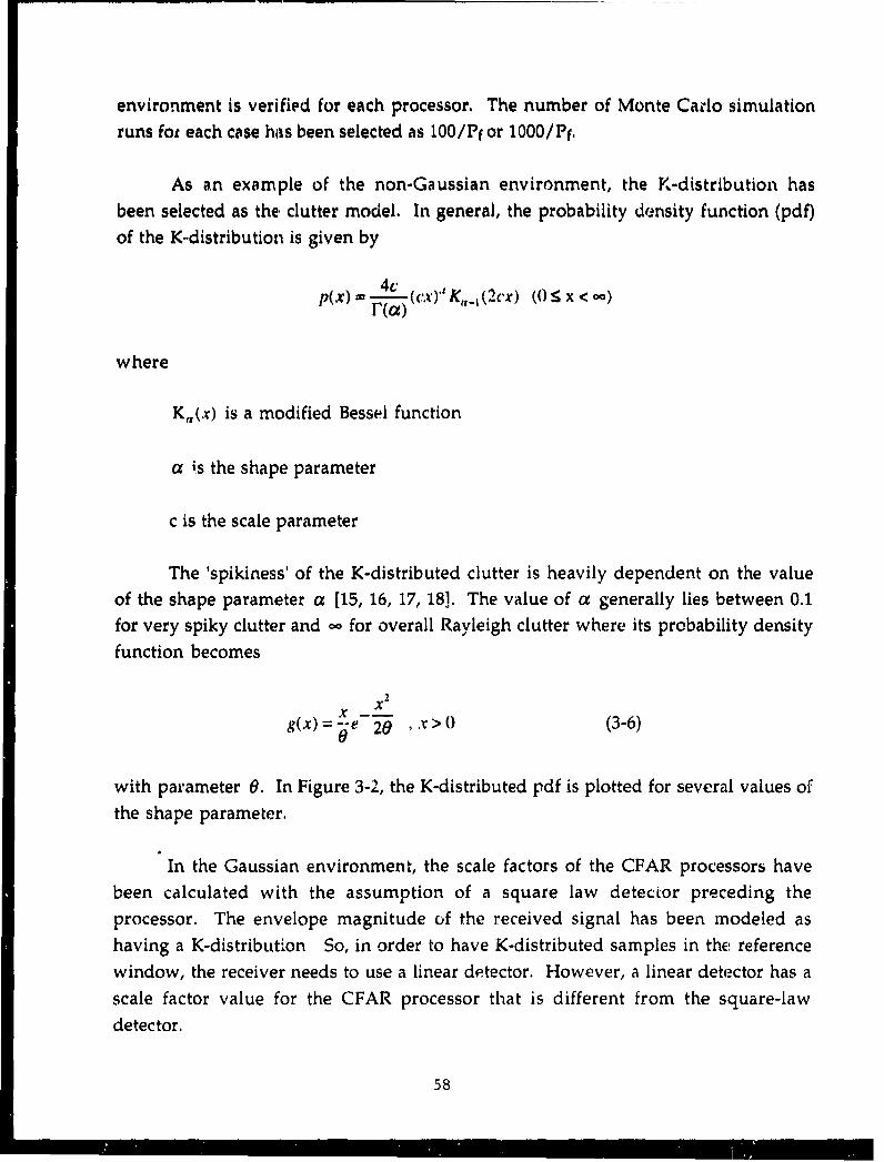
environment is verified for each processor. The number of Monte Carlo simulationruns for each case has been selected as 100/Pf or 1000/Pf.
As an example of the non-Gaussian environment, the K-distribution hasbeen selected as the clutter model. In general, the probability density function (pdf)
of the K-distribution is given by
41.p(x) -(cx) K,,.-1 (2cx) (0 : x < C,)
where
K,(x) is a modified Bessel function
a is the shape parameter
c is the scale parameter
The 'spikiness' of the K-distributed clutter is heavily dependent on the valueof the shape parameter a [15, 16, 17, 18]. The value of a generally lies between 0.1for very spiky clutter and cc for overall Rayleigh clutter where its probability density
function becomes
X2
X ' X
g(x)= -e 20 ,x>(> (3-6)
with parameter 9. In Figure 3-2, the K-distributed pdf is plotted for several values ofthe shape parameter.
In the Gaussian environment, the scale factors of the CFAR processors havebeen calculated with the assumption of a square law detector preceding theprocessor. The envelope magnitude of the received signal has been modeled ashaving a K-distribution So, in order to have K-distributed samples in the referencewindow, the receiver needs to use a linear detector. However, a linear detector has a
scale factor value for the CFAR processor that is different from the square-lawdetector.
58

I"R08AS I L'TY-.0 . f: • '4
OCNSITY,,,,-
20 ,
01.0
0.730,g0 -K. ./ ..,
4. ' 1 "
O, 1,.- , / N
- , / 4.\
0 . 00- /, ,,
- '4
0.10 0.35 O,8O 0.85 illO 1.35 1160 1,39 LAiO 2,35 2.60 2.85
CLUTTER AM,'PI.TTUE x
Figure 3-2: The K-distribution pdf for several values of the shape parameter. As
the shape parameter increases, the K-distribution approaches the
Gaussian condition (Rayleigh amplitude).
39
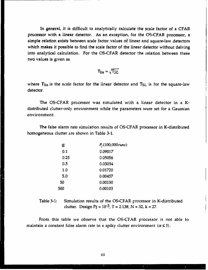
In general, it is difficult to analytically calculate the scale factor of a CFARprocessor with a linear detector. As an exception, for the OS-CFAR processor, asimple relation exists between scale factor values of linear and square-law detectorswhich makes it possible to find the scale factor of the linear detector without delvinginto analytical calculation. For the OS-CFAR detector the relation between thesetwo values is given as
Tuin =-" •T'S-L
where Tlin is the scale factor for the linear detector and TSL is for the square-lawdetector.
The OS-CFAR processor was simulated with a linear detector in a K-distributed clutter-only environment while the parameters were set for a Gaussianenvironment.
The false alarm rate simulation results of OS-CFAR processor in K-distributed
homogeneous clutter are shown in Table 3-1.
a P, (l00,0runs)
0.1 0.090170.25 0,05056
0.5 0.030341.0 0.017205.0 0.00457
50 0.00130
500 0.00103
Table 3-1: Simulation results of the OS-CFAR processor in K-distributedclutter. Design Pf = 10-3, T = 2.138, N = 32, k = 27.
From this table we observe that the OS-CFAR processor is not able tomaintain a constant false alarm rate in a spiky clutter environment (a < 5).
60

This simulation result is also in agreement with the result of the work done
by Armstrong and Griffiths [18]. In their analysis, they have also assumed a lineardetector and have shown that among CA-, CAGO- and OS-CFAR processors, the OS-CFAR processor is the most susceptible of the three to the effects of spiky clutter. Inthe homogeneous spiky K-distributed clutter environment, the CA-CFAR processoroutperforms the other two and the CAGO-CFAR processor lies between the CA andOS processors in terms of performance. But for the ultimate choice of the type ofCFAR processor to be used, other factors, such as the susceptibility to clutter edgesand interfering targets must be evaluated.
In the rest of this analysis, it is assumed that the CFAR processor is precededby a square-law detector so that the sample magnitudes are squared before they aresent to the CFAR processor.
In Section 3.2.1, the simulation procedure is explained. In Section 3.2.2 ,thesimulation results are given for homogeneous and non homogeneous background
conditions. In the homogeneous K-distributed clutter-only environment case, thesimulation error Confidence Interval curves are shown for both Pd and Pf versusthe shape parameter of the K-distribution.
3.2.1 Simulation Procedure
In the design of a CFAR processor, the threshold multiplier, T, is calculated interms of the given reference window size, N, false alarm probability, Pf, for the CA-CFAR and the CAGO-CFAR processors and in addition to the parameters given
above, the order number, k, for the OS-CFAR processor. A look-up table is made forthe threshold multiplier, T, for several values of the parameters given above.
Initially, assume that the clutter returns are much stronger than the Gaussiannoise so the samples from background consist only of K-distributed clutter returns.
The in-phase and quadrature-phase components of the complex low-pass K-distributed clutter signal is defined as
2= Zc +.jZs (3-7)
61
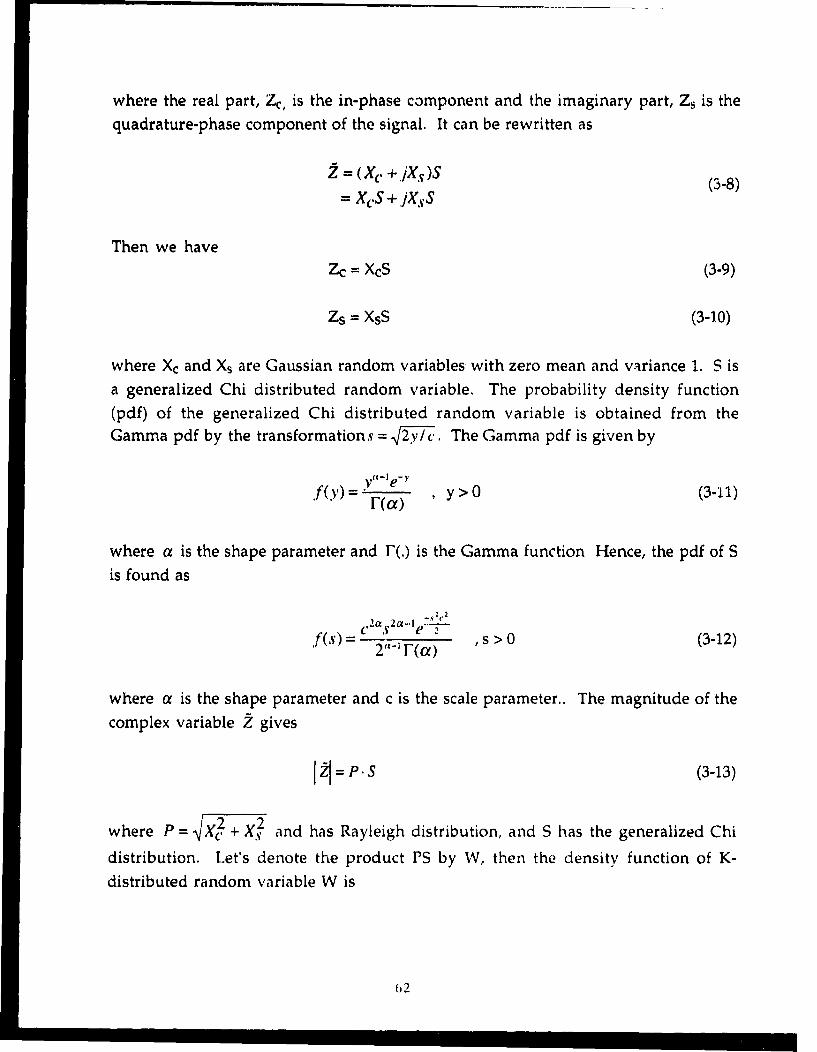
where the real part, Zc, is the in-phase component and the imaginary part, Zs is the
quadrature-phase component of the signal. It can be rewritten as
Z =(X. +,±Xs)S (3-8)= XC.S +jixS
Then we have
Zc = XcS (3-9)
Zs = XsS (3-10)
where Xc and Xs are Gaussian random variables with zero mean and variance 1. S isa generalized Chi distributed random variable, The probability density function
(pdf) of the generalized Chi distributed random variable is obtained from theGamma pdf by the transformations = V2y/c. The Gamma pdf is given by
.fy0) = - y>O (3-11)F(ca)
where a is the shape parameter and F(.) is the Gamma function Hence, the pdf of Sis found as
2 •,2-2 -ILLf(s)(a) , s > 0 (3-12)
where a is the shape parameter and c is the scale parameter.. The magnitude of thecomplex variable Z gives
Il=P.S (3-13)
where P = �2 + 2 and has Rayleigh distribution, and S has the generalized Chi
distribution. Let's denote the product PS by W, then the density function of K-distributed random variable W is
02

,lfLw)=-2 ._ 2 K,,-,(cw) , w >() (3-14)
where a is the shape parameter, c is the scale parameter and Kv(x) is the modified
Bessel function of the second kind.
As seen above, the magnitude of the clutter is a K-distributed randomvariable. In CFAR processors the magnitude of the sample is squared and then fedto the shift register.
In the simulation analysis, we have generated the K-distributed randomvariables, for a given shape parameter a, by generating Rayleigh and generalized
Chi distributed random variables arid then multiplying them as explained above.One of the features of CFAR structure is that the false alarm probability isindependent of the scale parameter of the homogeneous background distribution.
The target is modeled as a slowly fluctuating target, in which case the
magnitude of the signal returned from the target fluctuates from sample to sample.It is modeled as a Gaussian random variable. In the low-pass signal representationit becomes a complex Gaussian random variable. At the test cell, the sample is dueto the target-plus-clutter return. So
U=Uc +.jUs (3-15)= (Xct + JXst)+ (Xc +.Xs)S
where Xct and Xst are target signal components and are Gaussian random variableswith zero mean and variance a,;X,.X, and S, are clutter return components and are
the same variables as defined before. Then we have
U: = X,", + X,.S (3-16)
Us = Xst + X(S (3-17)
63
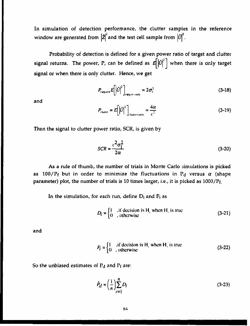
In simulation of detection performance, the clutter samples in the reference
window are generated from I 2 and the test cell sample from 101".
Probability of detection is defined for a given power ratio of target and clutter
signal returns. The power, P, can be defined as 4[0U2I when there is only target
signal or when there is only clutter. Hence, we get
P,,41.1] l = 2a-'" (3-18)
and
P'Itu,.r = E[I01 4a (3-19)
Then the signal to clutter power ratio, SCR, is given by
2 2SCR = 2 (3-20)2a
As a rule of thumb, the number of trials in Monte Carlo simulations is pickedas 100 /Pf but in order to minimize the fluctuations in Pd versus a (shapeparameter) plot, the number of trials is 10 times larger, i.e., it is picked as 1000/Pf.
In the simulation, for each run, define Di and Fi as
=I ifdecision is H, when H, is true (3-21)0i= . otherwise3-1
and
I .f decision is H, when H, is true (3-22)Fi 0 , otherwise3-2
So the unbiased estimates of Pd and P( are:
l= ()~i (3-23)
64
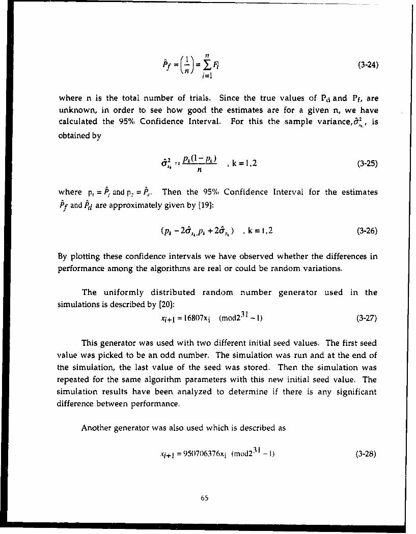
'1
Of Fi(3-24)i=1
where n is the total number of trials. Since the true values of Pd and Pf, areunknown, in order to see how good the estimates are for a given n, we havecalculated the 95% Confidence Interval. For this the sample variance, C^7,2, is
obtained by
" .-"L , k = 1.,2 (3-25)
where p, = P,. andp. =, . Then the 95% Confidence Interval for the estimates
Pf and Pj are approximately given by [191:
(p, - 20.,,.p, + 2a",,), k = 1,2 (3-26)
By plotting these confidence intervals we have observed whether the differences inperformance among the algorithms are real or could be random variations.
The uniformly distributed random number generator used in thesimulations is described by [20):
xi+l = 16807xi (mod231 - 1) (3-27)
This generator was used with two different initial seed values. The first seedvalue was picked to be an odd number. The simulation was run and at the end ofthe simulation, the last value of the seed was stored. Then the simulation wasrepeated for the same algorithm parameters with this new initial seed value. The
simulation results have been analyzed to determine if there is any significantdifference between performance.
Another generator was also used which is described as
Xi+l = 950706376xi (mod231 _ I) (3-28)
65

In all cases, the variations in the simulation results were found to be withinthe confidence intervals given before.
When the power level of the background Gaussian noise is comparable tothat of the clutter, the noise+clutter samples are generated by adding the in.-phaseand quadrature-phase components of a complex valued Gaussian random variableto the respective components of a complex valued K-distributed random variable.The test cell sample with a target can be generated by adding a complex valued
Gaussian random variable to the complex valued random variable given above. IfPptarget, Pitarget, Pclutter and Pnoise are the mean-square power levels of the primarytarget, interfering target, clutter, and noise respectively, then we define signal(primary target) to clutter power ratio, SCR, clutter to noise power ratio, CNR, andsignal to interfering target power ratio, SIR, as:
SNR = Ppt arg et / Pclutter (3-29)
CNR = Pelutter i Pnoise (3-30)
SIR = Ppt arget / Pitarget (3-31)
In the simulations the system parameter values have been selected as
Pf = 10- 3 (3-32)
N = 32 (3-33)
SCR = 10dB (3-34)
CNR = 5dB (3-35)
k =27 (for OS- CFAR) (3-36)
and the number of trials as
n = 1OO0/Pf = 1,000,000
66

3.2.2 5irnulatisn Results
In all performance plots in this section, the same legend was used for a givenCFAR processor. These legends are as follows:
lgn CFAR Processor
"square" OS(27)-CFAR
"star" CA-CFAR
"plus" GO-CFAR
"diamond" OS(32)-CFAR(iised only in non homogeneousclutter cases)
where 27 and 32 are the order numbers used for the OS-CFAR. In Pf performanceplots, the horizontal straight line without a legend on it shows the design Pf valuefor a Gaussian environment. Eight shape parameter values were selected to run thesimulations. These values are 0.10, 0.25, 0.50, 1.50, 2.50, 5.00, 10.00, 50.00 . Thesmaller values of the shape parameter correspond to spiky clutter and the largervalues correspond to nearly Gaussian clutter.
3.2.2.1 Homogeneous Background
In Figures 3-3 through 3-6, the Pf and Pd performance versus shape parameterof K-distributed clutter are shown for K-distributed clutter-only and K-distributed
clutter-plus-Gaussian noise homogeneous background conditions. SCR was chosento be 10 dB and CNR was equal to 5 dB.
In Figures 3-7 and 3-8, the 95% simulation error Confidence Intervals of the Pf
and Pd performance curves are shown for all CFAR processors.
67

PROBABILITY LFFA'.GE ALARM
.100 A.
.1 1. 00 0 .SHP PAAMTN
/ -- ,,"-.N
0.0f0 -of se68-
0.00 a~ function_____of shpprmee._hdsgn___ .0
- r-T---6r

PROBABILITY OFOETECTMI
0. s-
0.5-50.60 -
0.10-. -. 0 -0010.
SHAPE PARAMETER
CFAR PD PERFORMANCE IN HOMOGENEOUS K-CLUTTER-ONLY ENVIRONMENT
Figure 3-4: Probability of detection in homogeneous K-distributed clutter as a
function of shape parameter.
69

PROBABILI7't CV:FAL-SE ALARM
0. ICO --
0,0 '-,0.01.0
0.001
I~~~ I IT T T 7
0.1 1.0 10.0 100.0
SHAPE PARAMETER
CFAR PF PERFORMANCE D1 HOMOGENEOUS K+N -t1/IMONMh'tFT
Figure 3-5: Actual probability of false alarm in homogeneous K-distributed clutterplus Gaussian thermal noise as a function of shape parameter. Thedesign Pf is 0.001.
70

PROBABILITY OrF
D)ETECTIONd
0.55
"- \
0,50
0.35
0.30
0.25-
0. 20
0.1 1.0 10.0 100.0
SHAPE PARAHETER
CFAR PD PERFORMANCE IN HOMOGENEOUS K+rl Et'F,'tR4F.iiT
Figure 3-6: Probability of detection in homogeneous K-distributed clutter plusGaussian thermal noise as a function of shape parameter.
71
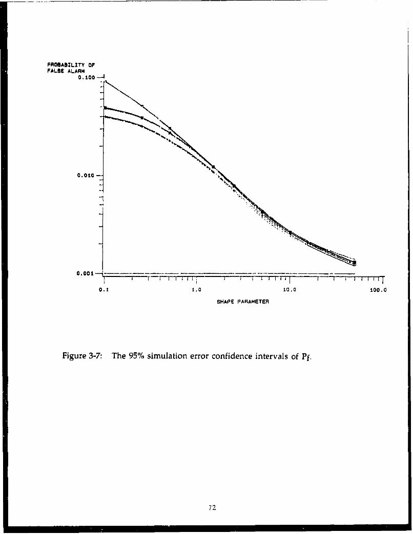
PROABIZLITY OFFALBE ALARM
o. iO0 -- 4
0.0100 --
0.01
M
O' I-" • I ~ J l Ii i t I ll l I Ii1 I1f
0.1 1.0 10.0 100.0
SHAPE PARAMETER
Figure 3-7: The 95% simulation error confidence intervals of Pf,
72

PROBABILITY OF~DETECTION
0.75
0.70
0.66
0.60
0.155
0.45
0.1 1.0 10.0 100.0
SHAPE PARAMETER
Figure 3-8: The 95% simulation error confidence intervals Of Pd.
73

3.2.2.2 Non homogeneovs Background
In this section, two cases of non homogeneous bac.kground conditions havebeen considered: multiple targets and non homogeneous clutter
Multiple Targets
In Figures 3-9 through 3-14, the Pf and Pd performances versus shapeparameter a of K-distributed clutter are shown for a K-distributed clutter-onlybackground condition with an embedded interfering target in it. As before, SCR waschosen to be 10 dB and CNR was equal to 5 dB. Three primary to interfering targetpower levels were considered: SIR = 5 dB, 0 dB and • I dB.
In Figures 3-15 through 3-20, the same cases were considered as in Figures 3-9through 3-14, but this time the background was filled with K-distributed clutter-plus-Gaussian noise instead of K-distributed clutter only.
Non homogeneous Clhtter
In this section, two different order numbers were used for each case of the OS-CFAR processor. That is k1=27 and k2=32.
In Figures 3-21 through 3-26, the Pf performances are shown versus a. Inthese cases, while some of the reference window cells were filled with point K-distributed clutter plus Gaussian noise, the rest were filled with only Gaussiannoise. This may happen if the clutter starts to occupy the reference window cellsone by one from one side. This scenario was assumed to be happening in thesesimulations which was important for GO-CFAR. For CA-CFAR and OS-CFAR, thelocation of the clutter within the reference window is not important. The test cell(TC) was assumed to be filled with only Gaussian-noise . CNR was equal to 10 dB.
The performances are shown fora values: 0.10, 0.25, 0.50, 1.50, 2.50, 5.00.
In Figures 3-27 through 3-32, the same conditions were repeated as in above,but this time the test cell (TC) was assumed to be filled with K-distributed clutter-plus-Gaussian noise.
74

PROBABZLI'Y CFFALSE ALARM
- N
IN
0. 0100-
0. 000 1, -7l, r • T -• I, T--7-7 -r, -- 71--T -i i i0.1 1..0 1.0.0 100.0
SHAPE PARAMETER
CFAR PF PERFORMANCES 114 K-CLUT.-ONLY EHIV. W•ITH I IIITF. TG.. S/I -5 OB
Figure 3-9: - Actual probability of false alarm in K-distributed clutter with oneinterfering target (S/SI = 5 dB). Design Pf is 0.001.
75

POBABIL: 7'( CFOETECTTb0I
0.65-- \
0.60-
.4
0.45 - .-
C 40 -
-4
0.35
0.0•-
0. 20 T -- '7
0.1 1.0 10.0 100.-
SHAPE PARAMETER
CFAR PO PERFORMANCE IN K CLUT. WITH I IhTF. T-,, S/4 - 5 D9
Figure 3-10: Probability of detection in K-distributed clutter with one interferingtarget(S/SI = 5 dB)
76

PROBABILITY OFFALSE ALARM
0. 1000
0.0010 --
-- 1
0.00010 1 Tk
. 0.10- 1.0 0.0_0.
----]...•--- --nr-r -rm-• F" ml-r-r-=r
SHAPE PARAMETER
CFAR PF PERFORMANCES IN K-CLUT.-ONLY EUV. WITH 1 I'TF. TG.. S/I "0 08
Figure 3-11: Actual probability of false alarm in K-distributed clutter with oneinterfering target (S/SI = 0 dB). Design Pf is 0.001.
77

PROBABILITY OFDETECTION
0.70-
-•1
0.65--\
0.55 \
0.502.
0.45
0.-0----
0. 35"-
0.30 -4
0. 25-•
0.20-• , r - r--r-T-1 -lTp -t i-F-F-F1] T -,•
0.1 1.0 10.0 100.0
SHAPE PARAMETER
CFAR PO PEFORMANCES IN K-CLUT.-ONLY ENV. WITH I IhTF. TG., 3/I / 0 08
Figure 3-12: Probability of detection in K-distributed clutter with one interfering
target(S/Si = 0 dB)
78
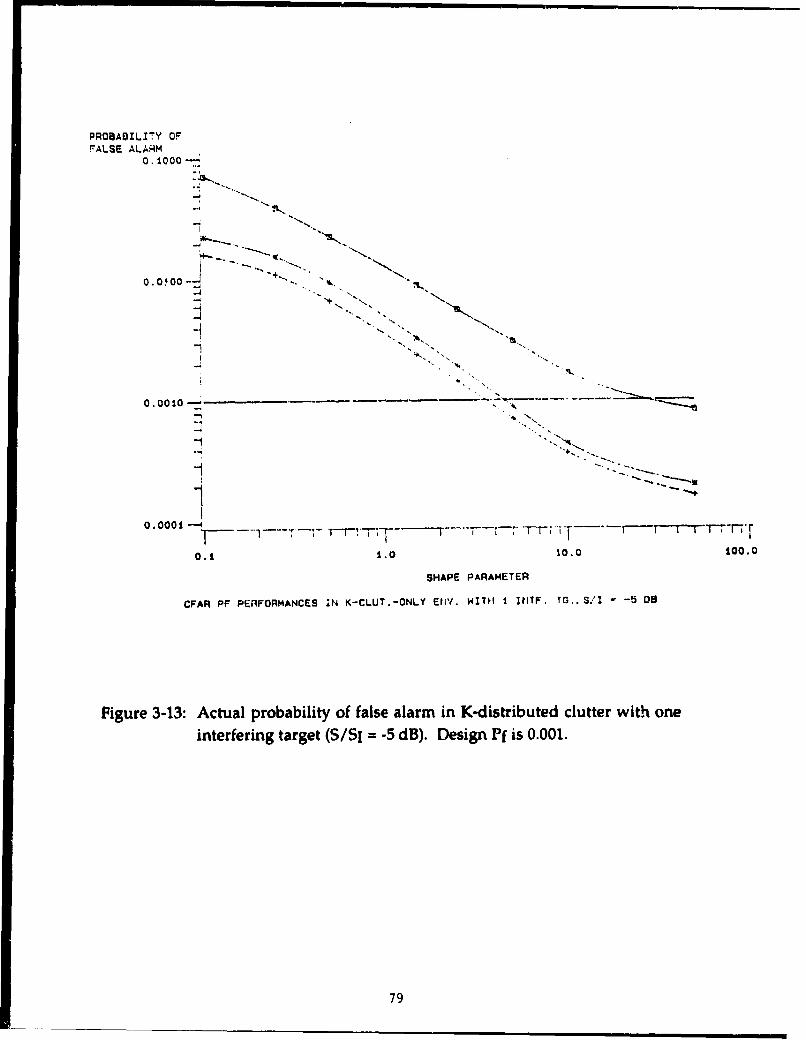
PROBABZL17Y OFFALSE ALARM
0. 1000
0.00010- T.
- N
"01 1.0 0.0
SHAPE PARAMETERCFAR PF PERFORMANCES 1N K-CLUT. -ONLY EtnV. WITH I !ItlTF. TG.. S."[ -5 08
Figure 3-13: Actual probability of false alarm in K-distributed clutter with oneinterfering target (S/SI = -5 dB). Design Pf is 0.001.
79
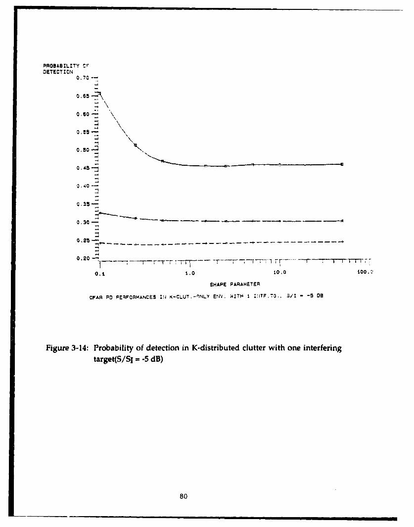
PROBABZLZTY Cr.OETECTICN
0,70--
0.50-0.55--
0.40 .0
-l
0,30 -
0.2-
-0,20- ----
0.1 1.0 10.0 too.:
SHAPE PARAMETER
CFAR PD PERFORMANCES IN K-CLUT.-INLY EIV. ' ITH I Z:ITF.T7.. S/I -5 - B
Figure 3-14: Probability of detection in K-distributed clutter with one interfering
target(S/Sl = -5 dB)
80

PROBABILITY OFFALSE ALARM
0, 1000
0.0100I
0.0001
0.1 1.0 10.0 100.0
SHAPE PARAMETER
CFAR PF PERFORMANCES IN K+N WITH I ItNTF. TGr.,,S/I -5 08
Figure 3-15: Actual probability of false alarm in K-distributed clutter plus Gaussiannoise with one interfering target (S/SI = 5 dB).
81
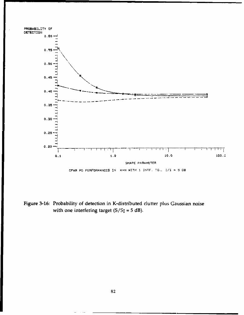
PROBABILITY OFDETECT I ON
0.60 -
o, .95 -l
O.5-I-s
0. 50 -.. ,
0. 45'-" "X-
0.40 7 "-.--. "_-
0. 35 --
0.30-
0.25 -
0.20 = 7r-'"
0.1 1.0 10.0 100.0SHAPE PARAMETER
CFAR PD PERFORMANCES IN K+N WITH I INTF. TG.. C/I - 5 DB
Figure 3-16: Probability of detection in K-distributed clutter plus Gaussian noisewith one interfering target (S/SI = 5 dB).
82

PROBABILITY OFFALSE ALARM
U. 1.000
-i
0.0100-, ,
.N.
.2 ..
0. 0010
0.1 1.0 10.0 100.0
SHAPE PARAMETER
CFAR PF PERFOR~MANCES IN. K+N WITH I INJTF. TG., S/I U OB
Figure 3-17: Actual probability of false alarm in K-distributed clutter plus Gaussiannoise with one interfering target (S/SI = 0 dB).
83

PROBABILITY OFDETECTION
-4
0.55-..
0.50
0.45
0.40 --
0.35-0, 5 --" - - - -,•- -- - ------ - --- ,•- -.
0.30
0. 25-
0.2011 -- Tr- --rr• - 1 r , F--I-i--rvj--r-----T-'r-r-'T
0.1 1.0 ±0.0 100.0
SHAPE PARAMETER
CFAR PD PERFORMANCES INI K+N WITH I INTF. TG,. S/I - 0 uB
Figure 3-18: Probability of detection in K-distributed clutter plus Gaussian noisewith one interfering target (S/SI = 0 dB).
84

PROBABILITY OFFALSE ALARM
0. 1000
0.0100
0.0010 .-
0,0001 ~I--' -rI -T-rr-rT 11---1 I II I I -I
0.1 1.0 1. 0.
SHAPE PARAMETER
CFAR PF PERFORMANCES ZN K+N WITH I ZNTF. TGT.. S/I -5 DO
Figure 3-19: Actual probability of false alarm in K-distributed clutter plus Gaussiannoise with one interfering target (S/SI = -5 dB).
85
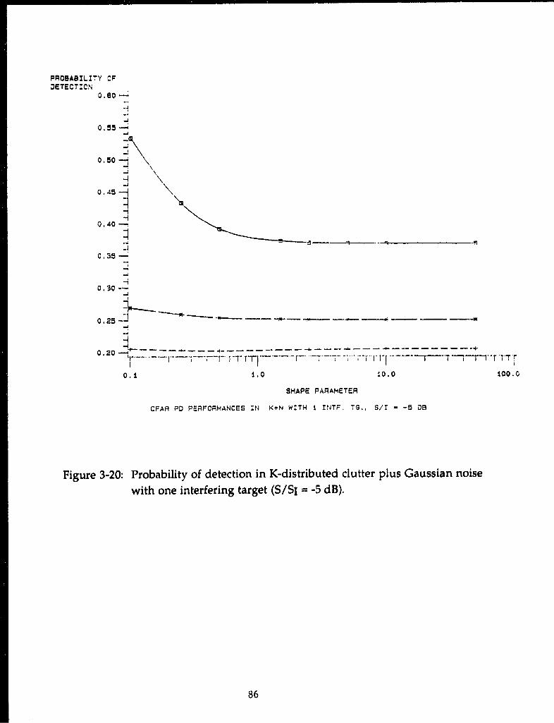
PROBABILITY OF•ETECT I CN
0. 80
0. 5
o so -•%
.-4
0,35 --
0.30 -0.20-,
0.5-"-- •----- ---- 1a
0 .. -. 0 0.0 100.0
SHAPE PARAMETER
CFAR PO PERFCRMANCES IN K+N W.TH I ;NTF. TG., S/I - -5 OB
Figure 3-20: Probability of detection in K-distributed clutter plus Gaussian noise
with one interfering target (S/SI = -5 dB).
86

PROBABILITY OFFAt.LBE AL.ARM
... O...O
.. .. ...
-• ,~~~~~~'I/") • ".i,'..
/
G o. 4..
0.01I II
NUMBER OF CELLS IN CLUTTER
CFAR PP IN PT CLUT. ENV..TCwN. SHP-O.1O. CLUT-K+N CL.AR-N, CNR-1O 09
Figure 3-21: Probability of false alarm as a function of the number of cells in K-
distributed clutter. Shape parameter is 0.10. CNR is 10 dB. Test cell is
in Gaussian noise only.
37

PROBABZLITY OFFALSE ALARM
0.00100
--
0. 00010
0.00001 rS 2 5 7
NUMBER OF CELLS IN CLUTTER
WAR PF IN PT CLUT. ENV..TCwN. SHP'O.25. CLUT-K÷N CLEAR-N, CNR-1O 05
Figure 3-22: Probability of false alarm as a function of the number of cells in K-distributed clutter. Shape parameter is 0.25. CNR is 10 dB. Test cell is
in Gaussian noise only.
88

PROBABZLZTY OFFALSE ALARM
0. 001000
0.000100
0,000010.
0.000001•
1- -
S • -
NUM4BER OF CELLS IN CLUTTER
WIAR PF IN PT CLUT. ENV.. TC-,N, SHP-0.50. CLUT-K+N CLEAR-N. CNA-10 016
Figure 3-23: Probability of false alarm as a function of the number of cells in K-dis00ibuted clutr. Shape parametr is 0.50. CNR is 10 dB. Test cell is
in G~aussian noise only.
89
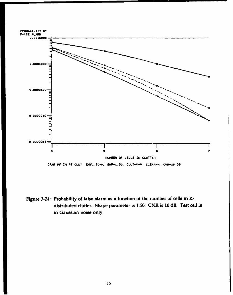
PROBABZLITY OFFALSE ALARM
0.0010000
0. 000 1000
o . o o o o , o _ _..N% N
o. oooooS. ,
0.001 IS I
0.0000100 -1 .-
2 7
NUMBER OF CELLS IN CLUTTER
CIFAR PF IN PT CLUT. ENV.. TC-N. SHP-1.50. CLUT-K+N CLEARI-N. CNR-10 08
Figure 3-24: Probability of false alarm as a function of the number of cells in K-0 distributed clutter. Shape parameter is 1.50. CNR is 10 dB. Test cell is
in Gaussian noise only.
90

PROBABILZTY OFFALSE ALARM
0.0010000
0.0001000
0.0000100 %
NUMBEIR OF CELLS IN CLUTTER
CFAR PF IN PT1 CLUT. eNV.. TCN. sHP=2.50. CL.UT-K+H CLEAR-N. CNR-10 Do
Figure 3-25: Probability of false alarm as a function of the number of cells in K-
distributed clutter. Shape parameter is 2.50. CNR is 10 d8. Test cell is
in G~aussian noise only.
91
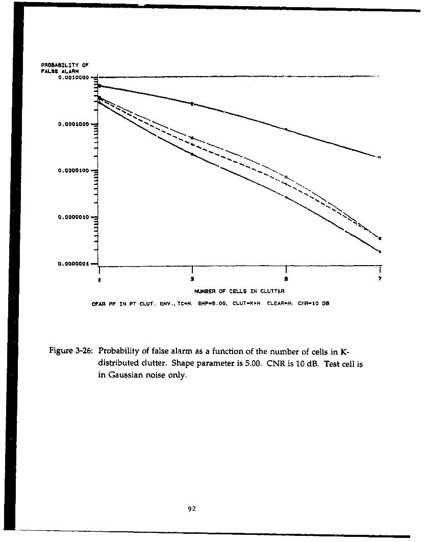
PROBABZLZTY OFFALBE ALARM
0.0010000 -
0.0001000
0.0000100 -% '-.,
0.0000010 --
S a0.00000014_ _ _ _ _ _ _ _ _ _
NUMBER OF CELLS ZN CLUTTER
CFAR PF ZN PT CLUT. ENV.. TC-N. SHP-5.00. CLUT-K+N CLEARN. CHR,10 OB
Figure 3-26: Probability of false alarm as a function of the number of cells in K-distributed clutter. Shape parameter is 5.00. CNR is 10 dB. Test cell isin Gaussian noise only.
92

PROBABZLITY OFFALSE ALARMS. 000
0. 100
- -- - - - - - - - - .---- - -- - - 4 . - - ---- -
t2
0.001 -3L2 26 13
17 20 NUMBER OF CELLS IN CLUTTER
CFAR PF IN PT CLUT. ENVt. TCK+N. SHP-0 . . CLUT-K÷N CLEAR"N, CNR-10 DO
Figure 3-27: Probability of false alarm as a function of the number of cells in K-
distributed clutter. Shape parameter is 0.10. CNR is 10 dB. Test cell is
in clutter plus Gaussian noise.
93
.. ••• .••

iPR3A0ZLZ7Y OF
FALSE ALARM1000
0.100 -
-.. - a- -a--- - ' a- -- -- -..
0.0100
0,001
23 15
t7 t o NU M B E R O F C E L LS I N C L U T T E R
CFAR PF IN PT CL.JT. t'tV., TcK+N- !PO' C.UTwK+N CLEAR-N, CHt"tO fB
Figure 3-28: Probability of false alarm as a function of the number of cells in K-
distributed clutter. Shape parameter is 0.25. CNR is 10 dB. Test cell is
in clutter plus Gaussian noise.
94

PROBABZLZTY OFFALSE ALARM
o. -SO0---
0.010
SIII I17 no 33 as to 32
NUMBER OF CELLS ZN CLUTTER
cFAR PF ZN PT CLUT. ENV..TC-K+N. SHP-0.50. CLUT-K+N CLEAR-N, CNR-1O 0s
Figure 3-29: Probability of false alarm as a function of the number of cells in K-distributed clutter. Shape parameter is 0.50. CNR is 10 dB. Test cell isin clutter plus Gaussian noise.
95
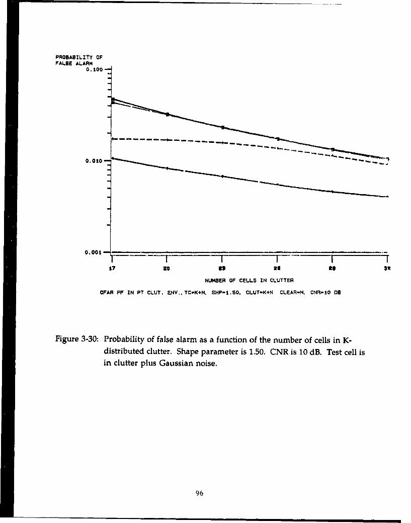
PROBABILZTY OFFALSE ALARM
0.100
O.O-O -"" "",-,-= .- - -"-
0.010 -. 7
O .O ~ . . .. .. "- -• ... . ,-
iiII I17 s0 33 to to 3W
NUMBER OF CELLS ZN CLUTTER
CFAR PF IN PT CLUT. ENV.. TCK+N. SHP-1.50. CLUT-K+N CLEAR-N. CNR-10 OB
Figure 3-30: Probability of false alarm as a function of the number of cells in K-distributed clutter. Shape parameter is 1.50. CNR is 10 dB. Test cell isin clutter plus Gaussian noise.
96
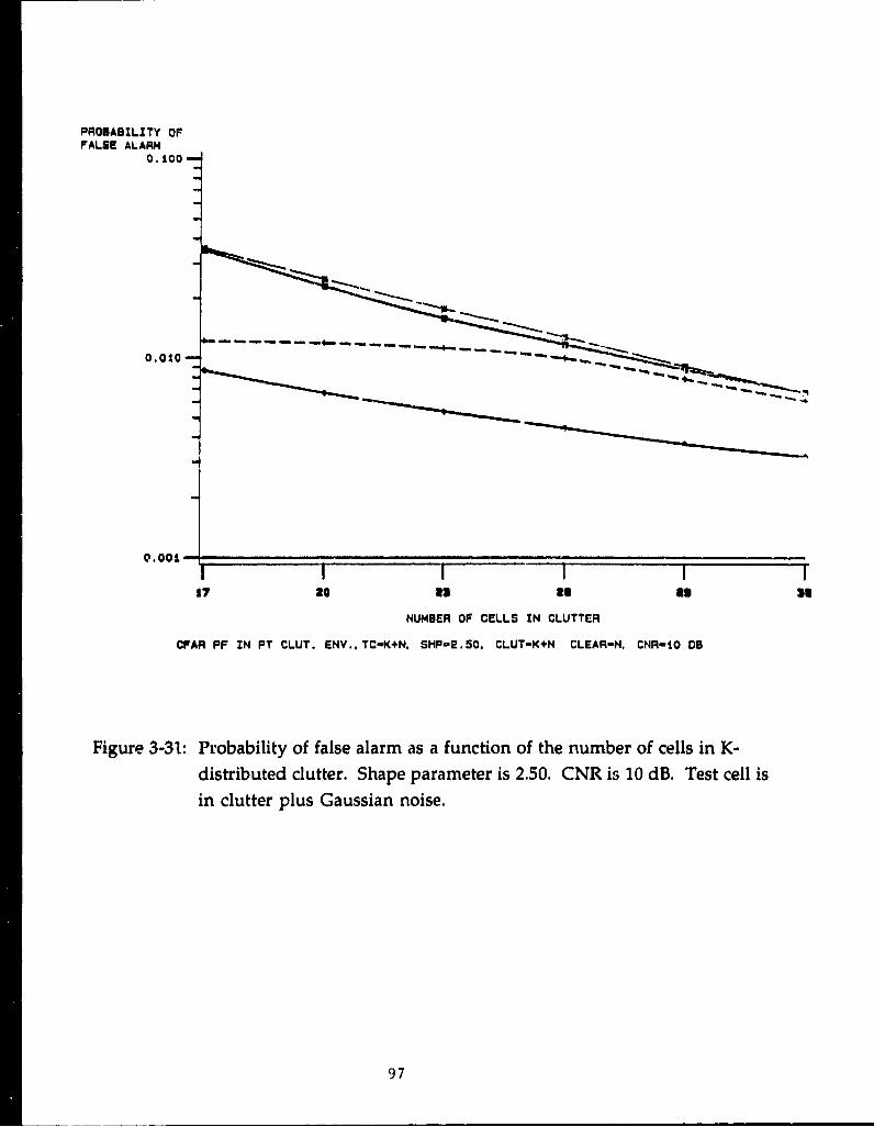
PROBABILITY OFFALSE ALARM
0.100
0.0 10 ~-
0.001 I I I II17 to as to a3 s3
NUMBER OF CELLS IN CLUTTER
CFAR PF ZN PT CLUT. ENV..TCaK+N. SHP-2.50. CLUT-K+N CLEAR-N. CNR-t0 05
Figure 3-31: Probability of false alarm as a function of the number of cells in K-
distributed clutter. Shape parameter is 2.50. CNR is 10 dB. Test cell isin clutter plus Gaussian noise.
97
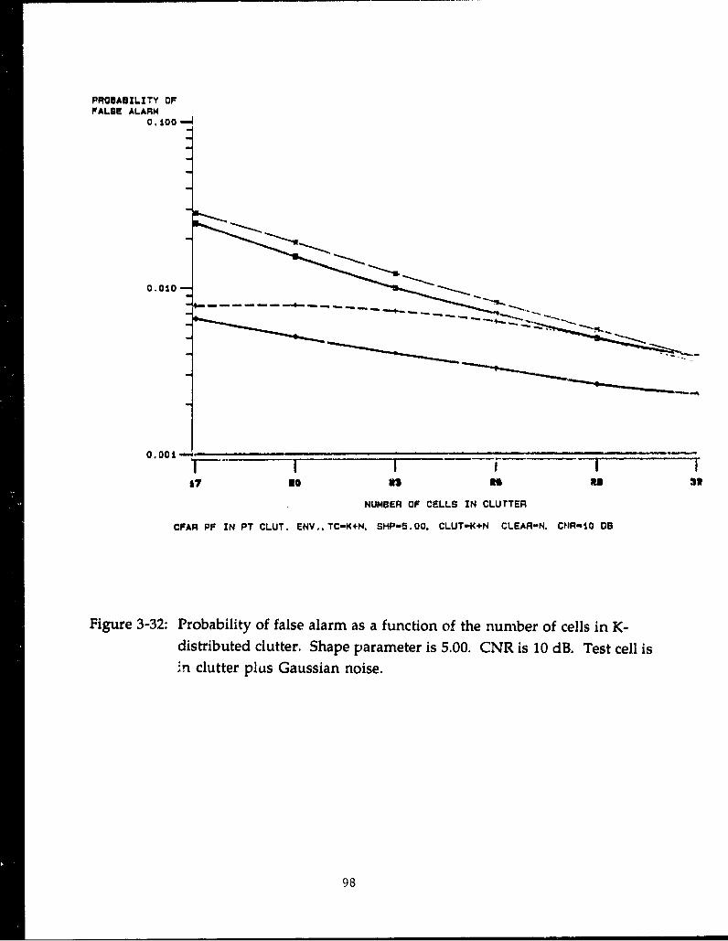
PROBABZLZTY OFFALSE ALARM
0. 100
o.oio • -
0.010 -,-.
T I I tI17 30 as 3233S
NUMBER OF CELLS IN CLUTTER
CFAR PF IN PT CLUT. ENV.. TC-K+N. SHP-5.00. CLUT-K+N CLEAR-N. CHR-10 09
Figure 3-32: Probability of false alarm as a function of the number of cells in K-distributed clutter. Shape parameter is 5.00. CNR is 10 dB. Test cell is
in clutter plus Gaussian noise.
98

Next, it was assumed that some of reference window cells were filled with K-distributed clutter plus Gaussian noise (K1+N) with CNR1=15 dB eind the rest werealso filled with K-distributed clutter plus Gaussiaii noise (K2+N') but with CNR2=5dB. The test cell (TC) was assumed to be in K1+N The Pf perforninces in thisenvironment condition are shown in Figures 3-33 through 3-40 for all eight shapeparameter.
3.2.2.3 Homogeneous Background with Different PF Design Values
in an attempt to bring down the Pf level of the CFAR processors in K-distributed clutter-only environment down to the desigced level (Pf = 10-3), scalefactors were varied for CFAR processcrs. These scale factors were calculated basedon a Gaussian-only environment assumption, for PF levels at 1)-3, 10-4,...,10-18.With these scale factors, the PF and PD performance versus shape parameter, in K-distributed clutter-only homogeneous background condition are shown in Figures3-41 through 3-46. SCR was equal to 10 dB. The results indicate that for smallvalues of a , extremely low design Pf rates must be used to achieve the moderate Pfrates obtained in a Gaussian environment. Unfortunately, this causes Pd to degradeto unacceptably low levels. In other words, it is not practical to vary the threshold ina non-Gaussian environment to achieve the same false alarm rate achieved in aGaussian environment, if the CFAR is designed using a Gaussian assumption.
These simulation results will be used to develop the decision rules for the ESCFAR system, to select the best CFAR processor with its parameters set at optimumvalues to maintain the desired constant false alarm probability while obtaining thehighest possible probability of detection.
99
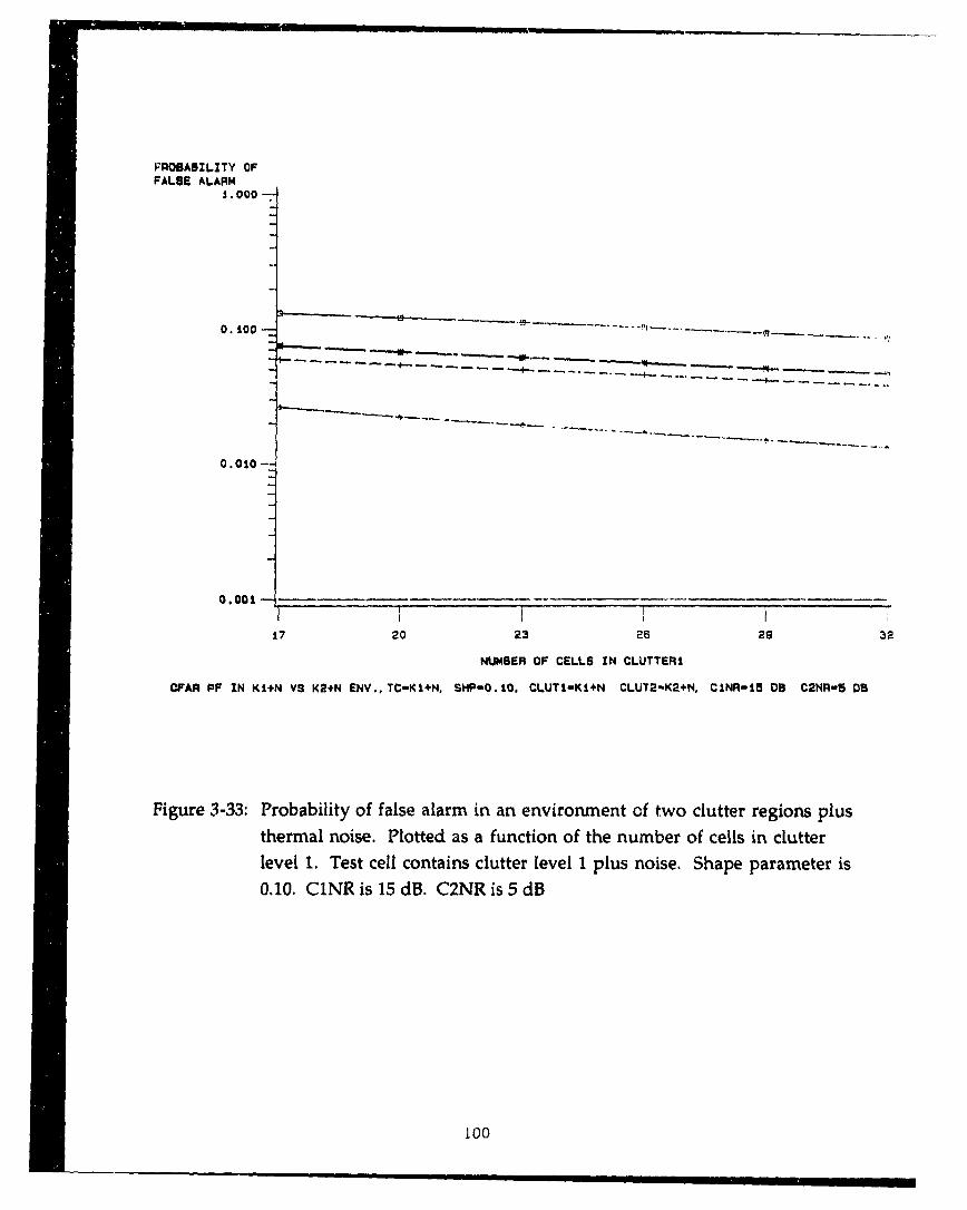
FROBABILZTY OFFALSE ALARM
0.000 -
* -
0.010
0.001- -- -___
17 20 23 26 29 32
NUMBER OF CELLS IN CLUTTERI
WFAR PF ZN KI+N VS K2+N ENV.. TCK1+N, SHP-0.1O. CLUTI-Kl+N CLUT2-K2+N. CINR-15 OB C2NR,5 DB
Figure 3-33: Probability of false alarm in an environment of two clutter regions plusthermal noise. Plotted as a function of the number of cells in clutter
level 1. Test cell contains clutter level 1 plus noise. Shape parameter is
0.10. C1NR is 15 dB. C2NR is 5 dB
100

PROBABILZTY OFFALSE ALARM
1.000 -
0.100 -----------------
~ --- -
0---------
3
O .0•0 --9
20 23 29
i"7 20
2
NU14SER OF CELLS IN CLUTTERI
CFAR PV %N KI+ H V S K2 04 ENV..TC"K 1*" SVp 0 . CLUT I-K1+N CLUT2 -K2. +N.
I R S 05 C N B
Figure 3-34: Probability of false alarm in an environment of two clutter regions plus
thermal noise, plotted as a function of the number of cells in clutter
level I. Test cell contains clutter level I plus noise. Shape parameter is
0O25. CNR is 15 dB. C2NR is 5 dB.
101

PROBABILITY OFFALSE ALARM
0.100-.
0.010--7
0.0•10
17 20 23 25 29 32
NUMBER OF CELLS IN CLUTTERI
CFAR PF IN KI+N VS K2+N ENV.. TC-KI+N. SHP-0.50. CLUTI-KI+N CLUT2-K2+N. CINR-15 0B C2NR-5 OS
Figure 3-35: Probability of false alarm in an environment of two clutter regions plusthermal noise. Plotted as a function of the number of cells in clutterlevel 1. Test cell contains clutter level 1 plus noise. Shape parameter is0.50. C1NR is 15 dB. C2NR is 5 dB.
102
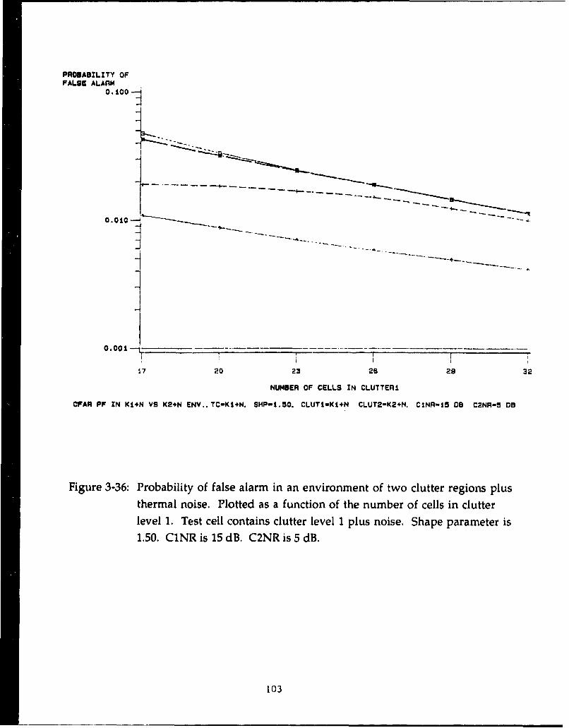
PROBABILITY OFFALSE ALARM
O). 0 --0
0.100
17 20 23 26 29 32
NUMBER OF CELLS IN CLUTTERI
ClFAR PF IN KI+N VS K24N ENV.. TC-KI+N. SHP-1.50. CLUTI-KI+N CLUT2-K2+N. C1NR-15 0B C2NR-5 05
Figure 3-36: Probability of false alarm in an environment of two clutter regions plusthermal noise. Plotted as a function of the number of cells in clutterlevel 1. Test cell contains clutter level 1 plus noise. Shape parameter is1.50. C1NR is 15 dB. C2NR is 5 dB.
103

PROIAZILZTY OFFALSE ALARM
0. 100 -
------ -- -- --------------4-------
0.010 -
0. 00 1
-7 -- 7
o~oo . .... _ .--..- - -4 -[
0NUMBER OF CELLS IN CLUTTERI
WAR PP ZN Kj÷N VS K2+,N ENV..TC-KI•N. SHP-2.50. CLUTI-KI+N CLUT2-K2+N. CINR-15 00 C2NR-5 OB
Figure 3-37: Probability of false alarm in an environment of two clutter regions plus
thermal noise. Plotted as a function of the number of cells in clutter
level 1. Test cell contains clutter level 1 plus noise. Shape parameter is2.50. C1NR is 15 dB. C2NR is 5 dB.
104
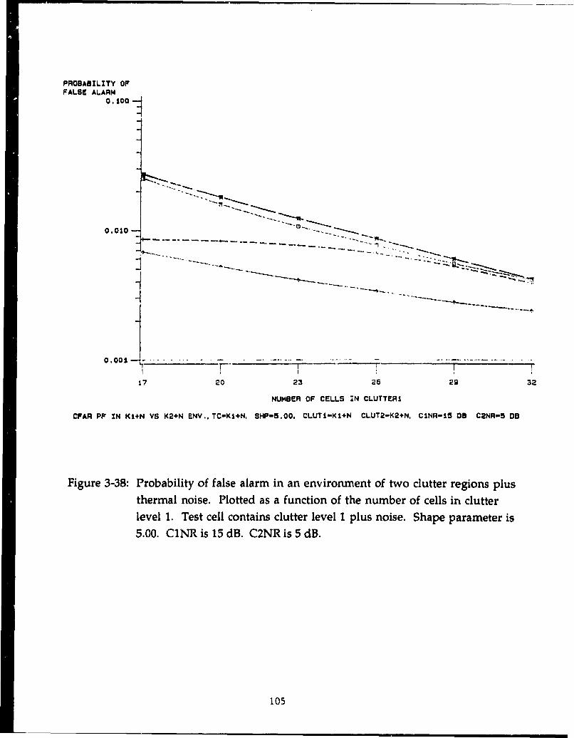
PROBABILITY OFFALSE ALARM
0.100 -.
0.010 -i
0.001 ......
17 20 23 26 29 32
NUMBER OF CELLS :N CLUTTERI
CWAR PF IN KI+N VS K2+N ENV.. TC-KI+N, SHP-5.00. CLUTI-KI+N CLUT2-K2+N. CINR-15 03 C2NR-5 00
Figure 3-38: Probability of false alarm in an environment of two clutter regions plus
thermal noise. Plotted as a function of the number of cells in clutterlevel 1. Test cell contains clutter level 1 plus noise. Shape parameter is5.00. C1NR is 15 dB. C2NR is 5 dB.
105
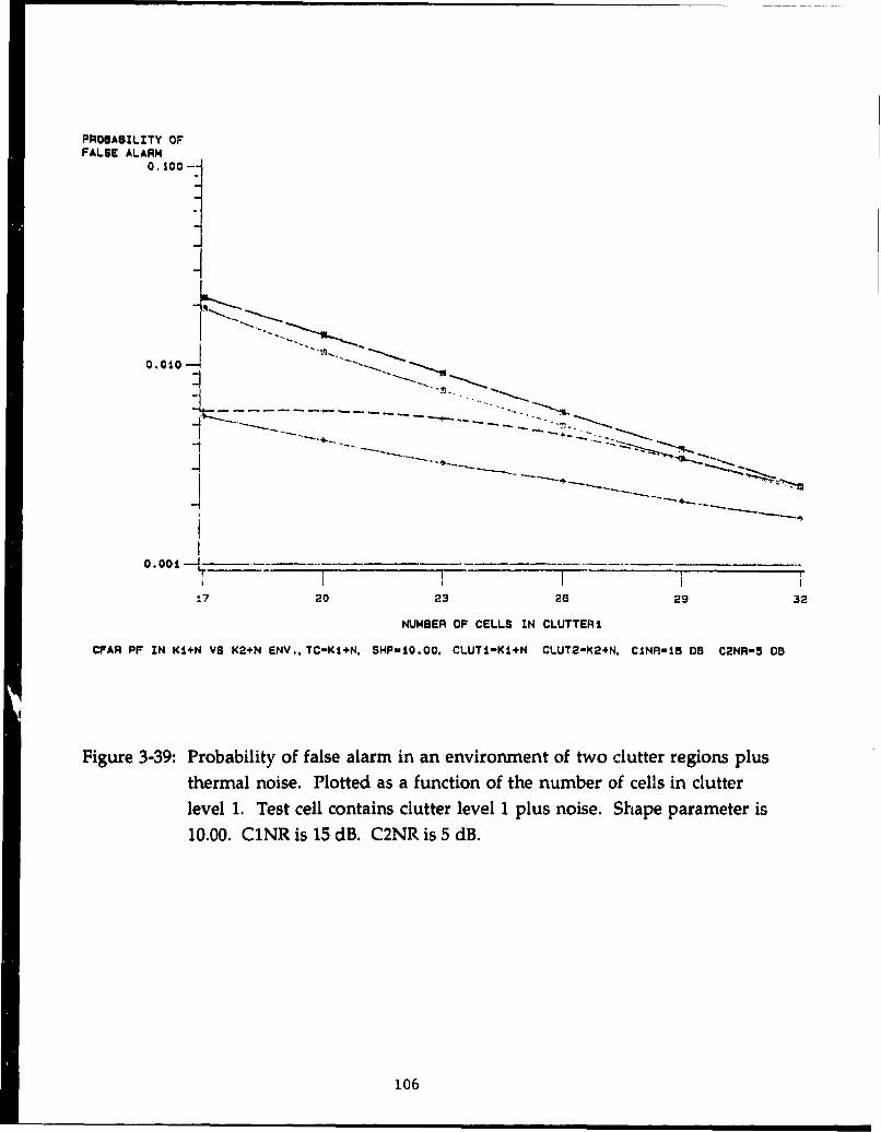
PROBABILZTY OFFALSE ALARM
0.100 --
0.010
0.0101
I -- .4
17 20 23 26 29 32
NUMBER OF CELLS IN CLUTTERI
CFAR PF IN KI+N VS K2+N ENV.,TC-K$+N. SHP-10.00. CLUTI-KI+N CLUT2-K2+N. CINR-15 0B C2NR-5 O0
Figure 3-39: Probability of false alarm in an environment of two clutter regions plusthermal noise. Plotted as a function of the number of cells in clutterlevel 1. Test cell contains clutter level 1 plus noise. Shape parameter is
10.00. C1NR is 15 dB. C2NR is 5 dB.
106

PROBAIZLZTY OFFALSE ALARM
0.100
0.010
OO -.--
17 20 23 26 29 32
NUMBER OF CELLS IN CLUTTERi
WFAR PF IN K1÷N VS K2+N ENV.. TC-KI+N. SHP,50.O0. CLUTI-Ki+N CLUT2-K2+N. CINR-15 05 C2NR-5 OB
Figure 3-40: Probability of false alarm in an environment of two clutter regions plusthermal noise. Plotted as a function of the number of cells in clutterlevel 1. Test cell contains clutter level 1 plus noise. Shape parameter is
50.00. C1NR is 15 dB. C2NR is 5 dB.
107
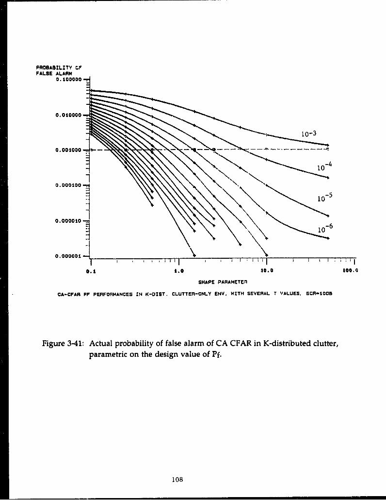
PROBABILITY CFFALSE ALARM
0. 100000
0.010000
0.00100 - U-- -- 10-3
0. 0001000 -
10-4
0.000010 - o 6
0.000001 _______________
@41.0 10.0 100.0
SHAPE PARAMETEA
CA-CFAR PF PERFORMANCES IN K-OIST. CLUTTER-ONLY ENV. WITH SEVERAL T VALUES, SCA-1005
Figure 3-41: Actual probability of false alarm of CA CFAR in K-distributed clutter,parametric on the design value of Pf.
108

PROBAUILITY OFOETECTIOI4
0. 75
0. 70
0. 65
0.60
0.50
0.45 1-
0. 40
0.30
0.20
0.1 1.0 10.0 100.0
SHAPE PARAMETER
CA-CFAR P0 PERFORMANCES IN K CLUT,-ONLY ENV. FOR SEVERAL T VALUES, SCR-10 08
Figure 3-42: Probability of detection of CA CFAR in K-distributed clutter,parametric on the design value of Pf.
109

PROBABILITY OFFALSE ALARM
0.100000
0.010000-
0.001000 -. - -- -. -- -- - - - -:-
0.0000 10
0.000001 __________________________
0.1 1.0 10.0 100.0
SHAPE PARAMETER
G0-CFAR PF PERFORMANCES IN K-DZST. CLUTTER-ONLY ENV. WITH SEVERAL T VALUES
Figure 3-43: Actual probability of false alarm of GO CFAR in K-distributed clutter,
parametric on the design value of Pf.
110

PROMAUZLITY OFDETECTION
0 75
0. 70
0.o65
0.60
0.55
0.50 10
0.45 -
0.40 -0-4
0.30 10''
0.25 10 -6
0. ao0
0.15 - %.*,.U -mg.-.- 0-5-
0.2- "" ""• ---- ---- -e-- -e-'--0- 0-
o I: ___-- --- * -0
0.10 2~...... -
0.05_
0.00 __ _ _ _ _ _ _ _ _ _ _ _ _ _ _ _ __W_ _ _ _ _ _ _ _ _ _ _ _ _ _ _ _ _ _
0.1 1.0 £0.0 100.0
SHAPE PARAMETER
00-CFAR PO PERFORMANCES IN K CLUT.-ONLY ENV. FOR SEVERAL T VALUES, SCR-1O 05
Figure 3-44: Probability of detection of GO CFAR in K-distributed clutter,parametric on the design value of Pf.
ll

"nOSABIITY OFiwAL8E ALARM
0. 100000
0.0', i "•"'"
0.010000A n -,,-° -"
IN ~103
0.000100 "-.0'5
0.000010 \\ '
IO, i '.0 1 10 0.i
SHAPE PARAMETER
OS-CFAR PF PERFORMANCES IN K-DIST. CLUTTER-ONLY ENV. WITH SEVERAL T VALUES
Figure 3-45: Actual probability of false alarm of OS CFAR in K-distributed clutter,parametric on the design value of Pf.
112

PROBABZLITY OFDETECTZON
0.70
0.65
0.50
0.55 \0.50 0- 3. f
0 .454
0.40 - \'-
0.35-
0.2a0.25 \
0.10 N.. -.....0. 00
o.o __-_ ___ _ ___o-
0. 1.0 -0. 00.
SMAPE PARAMETER
05-CFAR PO PERFORMANCES IN K CLUT.-ONLY ENV. FOR SEVERAL T VALUES. SCR-1o 09
Figure 3-46: Probability of detection of OS CFAR in K-distributed clutter,parametric on the design value of Pf.
113

4.0 SUMMARY OF TECHNICAL PROGRAM STATUS
This section summarizes the current program status and identifies near term
and longer range goals. In the long term this is a rather ambitious program which
uses Al techniques in virtually all aspects of radar signal data processing. As these
techniques become more widespread and the results become more accepted, many
approaches will evolve into (more or less) fixed algorithms. Others may remain in
the Al realm for quite some time since there will always be a need to operate in a
dynamic environment which can never be fully anticipated or characterized. It isthis ever changing environment, which normally requires human interaction, that
gives impetus to AT techniques. Whenever the environment is known
(deterministic) or can be completely characterized statistically, optimal strategies
either exist or can be developed. As always, near optimal strategies may actually be
of more value from an efficiency standpoint.
At the end of this current effort an expert system framework will beimplemented with an example system which focuses on CFAR processing. This
system will automatically examine the radar clutter environment, in ways similar
to what a human would do, and then select the optimal or near-optimal CFARwhich is judged most likely to be applicable. Notice that if the environment is
classified correctly and the proper CFAR algorithms are available then the goal of
maximizing the probability of detection while maintaining a constant false alarmrate will be achieved. It is unlikely that clutter will be classified correctly 100% of the
time, partly because some environments are too similar and partly becauseenvironments exist that do not fit into any of the pre-determined classes. An ideal
system would include all possible environments but this is obviously not practical.
An appropriate CFAR algorithm needs to be included in the CFAR library for each
anticipated environment. Currently, this library contains four algorithms: CA, GO,
OS, and TM. These four, with variations in their respective parameters, can be
utilized effectively in a large number of environments. At this time, additional
CFARs will probably not be added under the existing contract. However, it is verylikely that other CFARs will be added in the long term. The composition of the
software under this contract is being decided based on a compromise which attemptsto implement the most effective system given the available resources. The rest of
this section discusses the various compromises envisioned for each software area.
114

Radar Data Sources. To evaluate various heuristics the system must be capable of
creating the appropriate environment consisting of receiver noise, external noise,mixed clutter, and targets. Currently, receiver noise, Weibull clutter, log-normal
clutter, discrete clutter and Swerling I targets can be generated. By the end of thiscontract K-distributed clutter will also be included. This data is currently generated
in azimuth/range space. By the end of this contract Doppler space will also beadded. In the long term, the need for other clutter and target types is anticipated,including dynamic high fidelity RCS target models which would enable the system
to evaluate the use of adaptive waveforms for matched target illuminations. Thisshould be a very effective technique for detecting low RCS targets in heavy mixed
clutter.
In addition, by the end ot this contract recorded data will be injected into thesystem. In the long term it is likely that more types of recorded data as well as real-time data will be needed. Additionally, the capability to utilize multi-dimensionalCFAR's in range, azimuth, elevation and Doppler, would be desirable. The system
which will be completed under this contract, will perform CFAR processing in therange domain only.
Environmental Inp4utj. Currently no environmental inputs have beenimplemented. Under this contract the user is expected to be capable of specifyingregions of the simulated data to be area clutter such as land, trees, sea, etc. In the
long term, information pertinent to weather should be incorporated. This would beuseful in locating weather clutter, anomalous propagation, atmospheric layers,
ducting environments, etc. Also the addition of topographical data, while complex,may become feasible at some point in the future.
CFAR Selection Rules. Only a few rudimentary rules currently exist. This area is
the current focus of the effort and as such is not ready to be included in this report.By the end of this contract a comprehensive set of rules is expected to beimplemented, based on the extensive literature search completed earlier in theprogram and the simulations that have been performed. In the long term, as moreCFARs are added and after various experts have been exposed to this program, it isreasonable to assume that the CFAR selection rules data base will grow.
115
C.AR Pre-processot. Currently the CFAR pre-processor segments each radial intoregions made up of contiguous range samples which are similar statistically. Thisallows different CFARs to operate on different parts of each radial of data. Severaledge detection algorithms have been identified, including some used in digitalimage processing, and these are currently being tested. Spot detection algorithmsfrom digital image processing are also being considered to identify and tag isolateddiscontinuities which arise from targets, discrete clutter, noise glitches, etc. Thesepoints will be ignored by the CFARs except when they are actually in a test cell.Additionally, the pre-processor currently computes a list of statistics for each regionincluding mean, variance, skewness, kurtosis, mode, and correlation coefficient.These statistical estimates are used by the CFAR selection rules to help select theappropriate CFAR. In the long term the pre-processor can be expanded toimplement other non-linear transformations to facilitate optimal detection forspecific environments.
CFAR Library. The status of the CFAR library was summarized at the beginning ofthis section. In addition to those comments, any of the CFARs can be selected as thebaseline CFAR. All CFARs are currently designed assuming an exponential (power)clutter distribution. Under this contract the necessary code will be implemented toadjust the desired false alarm rate which is input to the ES CFARs to simulate othertail shapes. This empirically-derived adjustment will be based on the tail estimatorwhich is part of the CFAR pre-processor. In the long term, as additional optimalreceivers and clutter classification schemes are developed, the CFAR library isexpected to expand to include CFARs which assume a variety of tail shapes (ie: notjust the Gaussian assumption).
CFAR Post-processor. This is the software area where data fusion occurs and wherethe resultant candidate detections are processed using Al techniques to furthercontrol false alarms. The pre-processor attempts to standardize the radar data intomanageable environments. The CFAR selection rules then attempt to select themost applicable CFAR. When the environment adequately matches the CFARdesign assumptions, a constant false alarm rate will be maintained. In general,perfect knowledge is not available and perfect decisions are not always made (expertsmake mistakes), so as a result the false alarm rate will vary. By monitoring theactual false alarm rate and by utilizing confidence levels estimated in the pre-processor, the post-processor will trim the candidate detections when necessary to
116
better maintain a constant false alarm rate. Currently the post-processor isessentially a stub. First-order false alarm reconciliation is expected to be included bythe end of the contract. In the long term, the post-processor would include such
functions as track feedback, target library correlation, false alarm library correlation,and further tests to separate targets from false alarms.
Performance Measure. Currently, procedures are implemented to estimate Pd andPf for both the baseline and ES CFAR paths. For selected environments andrecorded data the desired Pf for the baseline CFAR can be adjusted until the actual Pf
for the baseline and ES CFARs are equal. Target RCS cart then be adjusted until thePd is equal for both. The dB change in target RCS will provide the desired quantifiedperformance measure. Of course the Pf for both channels prior to any adjustmentwill also serve as a performance measure, but it is not considered to be a stand-alonemeasure since it does not take into account the Pd. This process is expected to beautomated under this contract. In the long term it is expected that otherperformance measures would be put forth as more people become exposed to this
program.
Displays. Displays which are currently implemented include PPIs for both thebaseline CFAR channel and the ES CFAR channel, as well as a comparison PPI.Current displays also include the current radial of radar data vs. range, the estimatedPd and Pf for both channels vs. time, and the simulated clutter map. While itsgraphical user interface is elaborate, G2 has limited display capability for plotting
data. PV-WAVE 44 is being used to produce the power versus range plots as
shown in Section 2. Newer versions of G2 and PV-WAVE will be evaluated incoming weeks to automate the various displays. In the long term, additionaldisplays that illustrate variations with altitude should be included as well as target
track displays.
]17

REFERENCES
[1] P.P. Gandhi and S. A. Kassam, "Analysis of CFAR processors iin nonhomogeneous background," IEEE Transactions on Aerospace and Electronic
Systems, vol. 24, pp. 427-445, July 1988.
[2] Press, W.H., Flannery, B.P. Teukolsky, S.A., and Vetterling, W.T., 1988:"Numerical Recipes in C," Cambridge University Press, New York, 735 pp.
[3] Afifi, A.A. and S.P. Azen 1972: "Statistical Analysis, A Computer OrientedApproach," Academic Press, New York, 366 pp.
[4] H. M Finn and R. S. Johnson, "Adaptive detection with threshold control asa function of spatially sampled clutter-level estimates," RCA Review, vol.
29, pp. 414-464, September 1968.
[5] R. Nitzberg, "Analysis of the arithmetic mean CFAR normalizer forfluctuating targets," IEEE Transactions on Aerospace and Electronic Systems,
vol. 14, pp. 44-47, January 1978.
[6] R. Nitzberg, Application of invariant hypothesis testing techniques to signalprocessing. PhD thesis, Syracuse University, 1970.
[7) L. L. Scharf and D. W. Lyte, "Signal detection in Gaussian noise of unknown
level: An invariance application," IEEE Transactions on Information
Theory, vol. 17, pp. 404-411, July 1971.
[8] V. G. Hansen, "Constant false alarm rate processing in search radars," in
International Radar Conference, (London), pp. 325-332, IEE, 1973.
[9] J. D. Moore and N. B. Lawrence, "Comparison of two CFAR methods used
with square law detection of Swerling I targets," in International Radar
Conference, pp. 403-409, IEEE, 1980.
[101 J. Trickard and G. M. Dillard, "Adaptive detection algorithm for multiple
target situations," IEEE Transactions on Aerospace and Electronic Systems,vol. 13, pp. 338-343, July 1977.
118

(11] M. Weiss, "Analysis of some modified cell-average CFAR processors inmultiple target situations," IEEE Transactions on Aerospace and ElectronicSystems, vol. 18, pp. 102-113, January 1982.
[12] V. G. Hansen and J. H. Sawyers, "Detectability loss due to Greatest ofselection in a cell averaging CFAR," IEEE Transactions on Aerospace andElectronic Systems, Vol. 16, pp. 115-188, January 1980.
[1,] H. Rohling, "Radar CFAR thresholding in clutter and multiple targetsituations," IEEE Transactions on Aerospace and Electronic Systems, vol. 19,pp. 608-621, July 1983.
[14] G. V. Trunk, "Range resolution of targets using automatic detectors," IEEETransactions on Aerospace and Electronic Systems, vol. 14, pp. 750-755,September 1978.
[15] E. Jakeman and P. N. Pusey, "A model for non-Rayleigh sea echo," IEEETransactions on Antennas and Propagation, pp. 806-814, 1976.
[16] S. Watts, "Radar detection prediction in sea clutter using the compound K-distribution model," IEE Proceedings, Part F, vol. 132, pp. 613-620, December1985.
[17] S. Watts, "Radar detection prediction in K-distributed sea clutter andthermal noise," IEEE Transactions on Aerospace and Electronic Systems,vol. 23, pp. 40-45, January 1987.
[18] B. C. Armstrong and H. D. Griffiths, "CFAR detection of fluctuating targetsin spatially correlated K-distributed clutter," IEEE Proceedings, Part F, vol.138, pp. 139-152, April 1991.
[19] R. J. Larsen and M. L. Marx, An introduction to mathematical statistics andits applications. New York: Prentice-Hall. 1986.
[20] Z. A. Karian and E. J. Dudewicz, Modern statistical, systems, and GPSSsimulation. New York: Computer Science Press, 1991.
119

Appendix A
Summary of CFAR Literature Search
A-1

CFAR ALGORITHMS
The literature survey, discussed in the previous section, provided numerousreferences for many CFAR articles. A list of the abbreviations for the CFAR algorithms
encountered in the literature search is given in Table 1. For convenience in associatingan author or citation with a CFAR algorithm, a cross reference table is presented inTable 2. In the following subsections, a synopsis of CFAR algorithms is presented and a
candidate set of CFAR algorithms for selection by Al logic is derived.
SUMMARY OF IMPORTANT CFAR ALGORITHMS
The typical CFAR processing algorithm is shown in Figure 1. For pulsed Doppler
applications, the reference cells in a sliding window are used to estimate a backgroundnoise/clutter level. The power in the test cell is compared to a threshold, determined fromthe background clutter level and the desired false alarm rate. If the power in the test cellexceeds the threshold, a detection is declared. The sliding window can incorporate datafrom adjacent ranges, Doppler cells, or adjacent azimuths. In some CFARs, the cellsadjacent to the test cell (guard cells) are not used in the CFAR processing to avoidmasking effects that could occur in multiple target situations or when the target extends
through several range gates. For convenience, few references are given in the followingsubsections. The cross reference Table 2 can be used to determine literature citationsfor each type of CFAR.
Binary Integration
Binary integration (also called binary detection) is a simple detection method withrelatively good performance. Binary integration has the advantage of good performance
in non-Gaussian clutter environments. A set of N radar pulses are used in a double
threshold process. In the first threshold, the amplitude is compared to a threshold. In thea
second threshold, the number of times the first threshold was exceeded is compared to avalue M, less than N. If the sum of first threshold crossings exceeds M, a target isdeclared. The clutter envelopes Di, i = 1,2...,N are assumed to be independent andidentically distributed. An optimal value of M can be taken to be about 11.5NO.5 for a widevariety of conditions. Given M and the desired Pf, the threshold T can be determined if the
pdf of the D0 is known. The pdl is assumed to be exactly known. A Rayleigh pdf is often
A-2

Table 1. List of CFAR algorithm abbreviations.
Abbreviation Alias CFAR Algorithm
BI Binary IntegrationCA Cell AveragingCAGO GO Cell Averaging Greatest OfCCA Censored (excision) Cell AveragingCGO Censored Greatest OfCM Clutter Map
CMLD Censored Mean Level DetectorCVI Censored Video IntegratorDDL-GLR " Doppler Domain Localized Generalized Likelihood Ratio
DF NP Distribution FreeGCA Generalized Cell AveragingGLR Generalized Likelihood Ratio
GO Greatest Of
GST Generalized Sign Test
GTL-CMLD Generalized Two-Level Censored Mean Level DetectorHCE Heterogeneous Clutter Estimating
LOG LogarithmicLog-t Log-t detector
MGO Modified Greatest Of
MGST Modified Generalized Sign Test
MLD Mean Level DetectorMW Mann-Whitney
MX-CMLD Censored Mean Level DetectorMX-LCD Maximum Linear Combination Detector
MX-MLD GO Maximum Mean Level DetectorMX-OSD Ordered Statistic DetectorNP DF NonparametricOS OSD Ordered Statistic
OSo OS Ordered Statistic DetectorP PolarimetricSLC Side Lobe CancellingSMI Sample Matrix Inversion
SO Smallest OfSSA Scan by Scan Averaging
TM Trimmed MeanWH Weber-Haykin
A-3
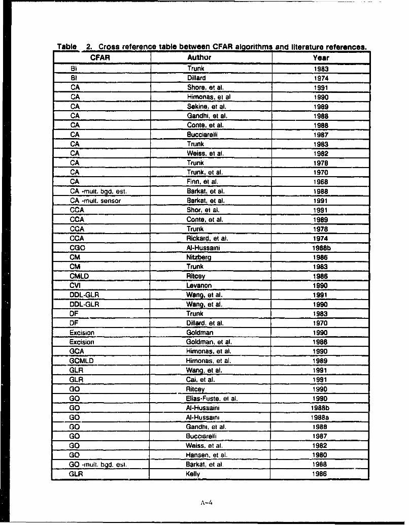
Table 2. Cross reference table between CFAR algorithms and literature references.
CFAR Author Year8l Trunk 1983BI Dillard 1974CA Shore, et al. 1991CA Himonas, et al 1990CA Sekine, et al. 1989CA Gandhi, et al. 1988CA Conte, et al. 1988CA Bucciarelli 1987CA Trunk 1983CA Weiss, et al. 1982CA Trunk 1978CA Trunk, et al. 1970CA Finn, et al. 1968CA -muit. bgd. est. Barkat, et al. 1988CA -mutt, sensor Barkat, et al. 1991CCA Shor, et al, 1991CCA Conte, et al. 1989CCA Trunk 1978CCA Rickard, et al. 1974CGO At-Hussaini 1988bCM Nitzberg 1986CM Trunk 1983CMLD Ritcey 1986CVI Levanon 1990DDL-GLR Wang, et al. 1991DDL-GLR Wang, et al. 1990DF Trunk 1983OF Dillard, et al. 1970Excision Goldman 1990Excision Goldman, et al. 1988GCA Himonas, et al. 1990GCMLD Himonas, et al. 1989GLR Wang, et al. 1991GLR Cai, et al. 1991GO Ritcey 1990GO Elias-Fuste, et al. 1990GO AI-Hussaini 1988b
GO AI-Hussainm 1988a
GO Gandhi, et at. 1988GO Bucciaretli 1987G0 Weiss, et al. 1982GO Hansen, et al. 1980GO -mult. b•d. est. Barkat, et al 1988GLR Kelly 1986
A-4

Table 2. Cross reference table between CFAR algorithms and literature references.(Continued)
CFAR Author YearGST Trunk, et al. 1974GST Hansen, et al. 1971GTL.CMLD Himonas, et al. 1990HCE Finn 1986LOG Novak 1980LOG Hansen, et al. 1972Log-t Goldstein 1972MGO Bucciarelli 1987a
MGO Bucciarelli 1987b-"MGST Trunk, et al. 1974
MLD Ritcey, et al. 1991MLD Rickard, et al. 1977MLD Dillard 1974MLD Steenson 1968MSMI Cai, et al. 1991MW Hansen, et al. 1971MX-CMLD Ritcey, et al 1991MX-LCD Ritcey, et al. 1991
MX-OSD Ritcey, et al. 1991
OS Shor, et al. 1991OS Elias-Fuste, et al. 1990DOS Levanon, et al. 1990
OS Sanile, et al. 1990OS Levanon, et al. 1990OS Lei, et al. 1989OS AI-Hussaini 1988cOS Blake 1988OS Rohling 1983Polarimetric Wanielik, et al. 1990bPolarimetric Wanielik, et al. 1990aPolynomial Nitzberg 1973Range-azimuth Martin 1976SMI Cai, et al. 1991SMI Wang, et al. 1990SO At-Hussaini 1988aSO Gandhi, et al. 1988SO Weiss, at al. 1982SO -muit. bgd. est. Barkat, et al. 1988SSA Lops, et at. 1989Sign test Hansen, et al. 1971TM Gandhi, et al. 1988WH Levanon, et al. 1990WH Weber, et al 1985
A-5
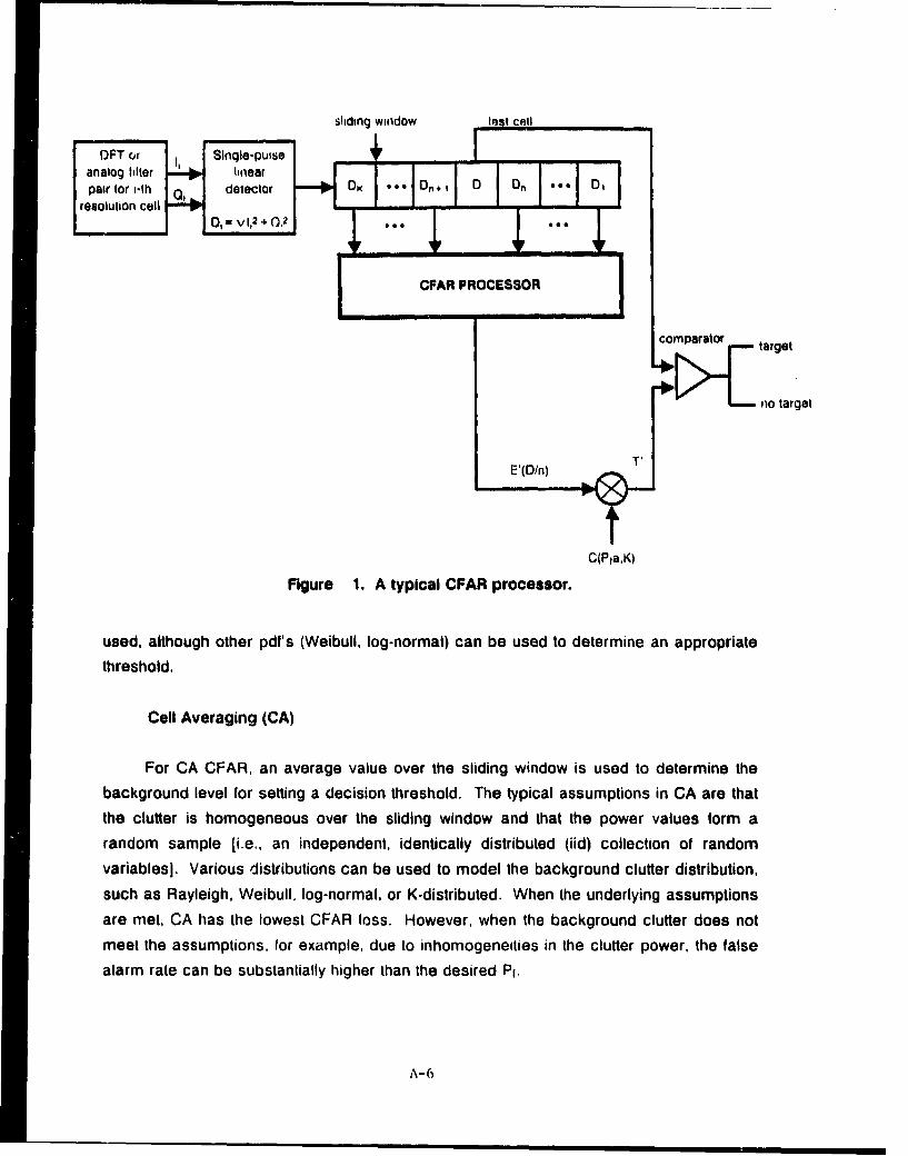
sliding window test call
analog filtnr tlinearpair for th detector pfK ( Wibunl I c b Dn a p opDt
resolution cellO0= Vl,2 +Q,2,,**
CFAR PROCESSOR
Cel veain (A
comparator the'1oo target
If ~~Figure 1. A typical CFAR processor. C~aK
used, although other pdr's (Weibull, log-normal) can be used to determine an appropriate
threshold.
Cell Averaging (CA)
For CA CFAR, an average value over the sliding window is used to determine the
background level for setting a decision threshold. The typical assumptions in CA are that
the clutter is homogeneous over the sliding window and that the power values form a
random sample [i.e., an independent, identically distributed (iid) collection of random
variables]. Various distributions can be used to model the background clutter distribution,
such as Rayleigh, Weibull, log-normal, or K-distributed. When the underlying assumptions
are met, CA has the lowest CFAR loss. However, when the background clutter does not
meet the assumptions, for example, due to inhomogeneities in the clutter power, the false
alarm rate can be substantially higher than the desired Pr.
A-6

Censored CA (CCA)
Censored CA is a variation of the basic cell averaging (CA) CFAR, proposed by
Rickard and Dillard (1974) to address the problem of masking by multiple targets. The
envelope values D, are ranked and the k largest values are censored from the sliding
window. The normal cell averaging procedure is then followed on the censored sample.
The excision CFAR procedure, described by Goldman and Bar-David (1988) is not
significantly different than CCA is its processing or assumptions.
Censored Greatest Of (CGO)
The Greatest Of (GO) CFAR is described in later section. The CGO is a variation of
GO, suggested by Weiss (1982). GO works well for clutter edges but suffers when
interfering targets are present. In CGO, the k largest values are censored from each side
of the split sliding window. As long as the number of interfering targets in each window is
less than k, CGO works better than GO. However, additional losses are incurred due to
the smaller sample size.
Clutter Map (CM)
The sliding window commonly used for CFAR consists of adjacent range and
Doppler cells. Clutter map CFAR uses previous values at the same range cell for the
sliding window. This is appropriate when the envelope data are inhomogeneous in range
or in adjacent Doppler cells. To reduce memory requirements, the method proposed by
Nitzberg (1986) uses a exponentially smoothed estimate from previous scans. CFAR loss
decreases with longer memory in the exponential filter. Losses vary from about 0.3 dB for
a weight of 0.98 to over 15 dB for a weight of 0.125.
Censored Mean Level Detector (CMLD)
The censored mean level detector (CMLD) is a variation of MLD that uses censoring
to reduce the effects of a nonhomogeneous clutter/noise environment. In CMLD, the k
largest noise samples are discarded prior to sample averaging.
A-7
Censored Video Integratcr (CVI)
Video integration is a noncoherent averaging of radar signal amplitudes. In
censored video integration, only the k smallest samples are included in the average. The
first k-1 are given unit weight while the kth sample is weighted by N - k + 1 to give aunbiased, minimum variance estimate of the average. CVI was proposed as acompromise to the complication of ordered statistics. Censoring incurs additional CFARlosses, on the order of several dB. CVI performance degrades if the number of interfering
targets is larger than the number of censored cells.
Doppler Domain Localized Generalized Likelihood Ratio (DDL-GLR)
Doppler domain localized generalized likelihood ratio (DDL-GLR) is a CFARalgorithm to efficiently detect moving targets in strong clutter with a complicated spectrum.
DDL-GLR assumes that measurements are available to estimate unknown clutter
statistics. DDL-GLR operates on the Fourier transform of the I and Q samples. For DDL-GLR, areas where the spectrum is rapidly changing are delineated [termed regions ofdetection improvement (RODIs)]. A GLR algorithm is then applied within these regions.DDL-GLR assumptions are identical to those for GLR, i.e., the data is divided into primary
and secondary sets. The secondary data are assumed to have noise and clutter only (notargets) while the primary data set could have a target. The covariance matrix is
estimated from ihe secondary data set. The noise plus clutter is assumed to have acomplex Gaussian distribution.
Distribution Free (DF)
Distribution free detectors are usually equivalent to nonparametric detectors in theengineering literature (Kassam, 1980). The discussion of these methods is in the &ection
on nonparametric methods.
Generalized Cell Averaging (GCA)
Generalized cell averaging (GCA) is a variat in on the ubiquitous CA CFAR. A basicassumption under CA is that the data in the r.ference (sliding) window are independent
and identically distributed. For the practical situations of weather clutter or chaff, thesamples may be correlated. When the samples in the reference window are correlated,
A-8

the normal CA procedure estimates a threshold that is too high. In the GCA study by
Himonas, et al. (19901, the elfects of spatial correlation of the samples in the reference is
modeled as a first-order Markov process. The covariance matrix is estimated from the
reference window, GCA can thus adapt to the actual correlation structure of the clutter.
Generalized Censored Mean Level Detector (GCMLD)
The presence of interfering targets in the reference windows can raise the threshold
too high in many CFAR algorithms and result in masking of targets. GCMLD is a
modification of CMLD that estimates the number of interfering targets and censors them
from the reference sample. A Swerling 2 target in a white Gaussian background is
assumed. A sequential censoring procedure is applied to the leading and lagging
windows to remove the samples from the interfering targets.
Generalized Likelihood Ratio (GLR)
Generalized likelihood ratio (GLR) is an adaptive procedure for detecting targets.
Two sets of input data are considered. First, the primary data set may contain a signal;
the secondary data set is assumed to contain only noise or clutter. The covariance matrix
for both data sets are assumed to be the same. A likelihood ratio is then formed of the
maximum likelihood function under the hypothesis of no target to the maximum likelihood
function under the hypothesis of a target. If the ratio exceeds some threshold, a target is
declared. The primary and secondary data are assumed to iid complex Gaussian
variates. GLR was found by Cai and Wang (1991) to offer more robust performance than
SMI when the background was colored Weibull or log-normally distributed.
Greatest Of (GO)
Greatest Of (GO) CFAR is a modification of CA to minimize effects of clutter edges.
The cells in the reference window is split into leading and trailing sets. The average value
is estimated for both sets. The parameter for determining the clutter distribution and the
CFAR threshold is selected as the maximum of the two averages from the leading and
trailing haif-windows. GO thus provides some control of Pf in clutter edges with relatively
small CFAR !oss over that of CA. However, an interfering target in one of the half-windows
decreases Pd intolerably and the target is masked.
A-9

Generalized Sign Test (GST)
The generalized sign test (GST) counts the number ot times the value in the test cell
exceeds the M values in the reference window during the N observation intervals in a CPL.
The number of times the N test cells exceeded the M reference cells is compared to a
threshold and a detection declared if it exceeds the threshold. The threshold value can
be set to provide the required Pf. GST assumes the N test cell values and the NxM
reference cell values are independent and identically distributed.
Generalized Two-Level Censored Mean Level Detector (GTL-CMLD)
GTL-CMLLJ is an extension of CMLD to model both nonhomogeneous clutter andinterfering targets. The data from the reference cells are ranked by magnitude and then
processed by a two-level censoring algorithm. For the first censoring level, a
determination is made whether the test cell is in the noise or the clutter. The other type is
censored from the reference cells. For the second level of censoring, the number of
interfering targets is determined and censored from the reference cells. The remaining
cells form the estimate of the clutter/noise level in the test cell.
Heterogeneous Clutter Estimating (HCE)
The heterogeneous clutter estimating CFAR is a modification of CA and assumes
that a heterogeneous clutter field can be represented as two homogeneous clutter fields
with different levels. The transition cell between the fields and the clutter levels in the two
fields is estimated. Research on the use of HCE showed that inevitable errors in the
location of the transition cell can place the test cell in the wrong clutter field and lead to
false alarms or missed detections. A biased version, that favors placing the test cell in
the more intense clutter field, appears to help.
Logarithmic (LOG)
Generally, LOG CFAR applies the cell averaging technique to samples from a
logarithmic detector, The advantages of logarithmic detection are the larger dynamic
range and normalization of data by subtraction rather than division. The disadvantage of
LOG CFAR is that the CFAR loss is higher than linear for the same number of cells in the
reference window.
A-10

Log-t Detection
The log-t detector maintains a constant false alarm rate when the clutter cells are
distributed log-normally or Weibull. The clutter is assumed to be homogeneous (identicallydistributed) and independent. As with most CFAR algorithms, the reference window caninclude range and/or Doppler cells. A test statistic, based on the difference between the
test cell and the average over the reference window in log space, is compared to athreshold. If the test statistic exceeds the threshold, a detection is declared. The log-tname is suggested because of the log transformation and the fact that it has a Student.t
distribution when the clutter is log-normal. Goldstein (1971) shows that the log-t statistic isindependent of the scale and shape parameters of the Weibull distribution.
Modified Greatest Of (MGO)
The modified greatest of (MGO) CFAR uses the standard GO technique but with an
estimated value of the Weibull shape factor from the reference window.
Modified Generalized Sign Test (MGST)
MGST is a modification of GST to control the false alarm rate in correlated andnonhomogeneous clutter. The first part of the CFAR processor, as described by Trunk. etal., (1971), is similar to the GST, described above, but implemented in hardware. A twothreshold technique is used to control false alarm rate. The first threshold is set for a Pf of10-6 when the clutter data are actually independent and identically distributed. Thesecond threshold is claimed to estimate the standard deviation of the cells in thereference window and to remove extraneous targets from the reference window. The
summary of the Trunk article notes that preliminary results are encouraging but that no
quantitative statements can be made yet.
Mean Level Detector (MLD)
The mean level detector provides an adaptive estimate of the background noiselevel by the sample mean of surrounding reference samples. MLD was originallyimplemented as a thresholding circuit for a short pulse noncoherent radar. MLD assumes
a homogeneous reference channel, consisting of square-law detected Gaussian noise
samples, all with the same variance as the test cell.
A\- I

Modified Sample Matrix Inversion (MSMI)
In MSMI, the sample matrix inversion technique is modified to allow for colored
Gaussian clutter. An analysis by Cai and Wang (1991) shows that MSMI and GLR offer
the same performance when the clutter has a Gaussian distribution. MSMI is easier to
implement than GLR. However, GLR has better performance when the clutter has a non-
Gaussian distribution, such as Weibull or log-normal.
Mann-Whitney (MW) Detector (Two Sample Wilcoxoli)
The Mann-Whitney detector is similar to GST and counts the number of times the
value in the test cell exceeds values in the reference cells. However, the Mann-Whitney
detector compares a given test cell to all of the reference cells in the CPI. The total count
is compared to a threshold and a detection declared if it exceeds the threshold. The
threshold value can be set to provide the required Pl. The Mann-Whitney detector
assumes the M test cell values and the NxM reference cell values are independent and
identically distributed. The Mann-Whitney detector has better performance than GST but
with a more complex design.
Maximum Family (MX) of CFAR Detectors
Several types of CFAR detectors that use a maximum of 2 local clutter level
estimates have been considered by Ritcey, et al. (1991) for false alarm control at clutter
edges. MX mean level detection (MX-MLD) is equivalent to GO. In MX censored mean
level detection (MX-CMLD), winsorized (Ritcey, op.cit, Eq. 5) mean estimates are used for
the 2 reference half-windows. For MX ordered statistic detection (MX-OSD), the maximum
of the quartiles for the two half-windows is used to treat interfering targets. Collectively,
these detectors are referred to as MX linear combination detectors (MX-LCD). The local
estimates for the two hall-windows are weighted linear combinations of the data in the
reference cells. The reference cell samples are assumed to be iid A simulation
comparison shows that MX-CMLD and MX-OSO are similar in performance. MX-OSD is
more complicated because of the need for sorting and has slightly higher loss.
A-12

Nonparametric Detectors (NP)
Nonparametric CFAR techniques are used to provide a constant false alarm rate
when the clutter or background noise statistics are unknown. Nonparametric and
distribution-tree techniques are taken to be equivalent in the CFAR literature, although thisis not strictly true. As with most CFARs, NP methods involve computing a detection
statistic from the reference cells, which is then compared to a threshold. Typically, NP
methods make only weak assumptions about the clutter, such as that the samples areindependent, identically distributed with known median. Two NP methods are the sign test
and the Wilcoxon detector. These can't be applied to radar detection because ofpractical considerations (i.e., the median level and the phase are unknown). For CFAR,
the generalized sign test and the Mann-Whitney detector are used. These CFARs are
described in their separate sections.
Ordered Statistic (OS)
Ordered statistic (OS) CFAR uses ordered statistics to improve performance with
clutter edges and interfering targets. The data in the reference cells are ranked and thekth largest sample is used for forming the detection threshold. For large values of k, OS
can control the false alarm rate similarly to GO but with lower detection efficiency. The
performance of OS with interfering targets is similar to SO. For determining the threshold,the samples from the reference cells are assumed to be independent, identicallydistributed. Various distributions have been considered, such as exponential (for squarelaw detection), Rayleigh, and Weibull. Typical CFAR losses as compared to CA are
small, about 0.5 dB.
Polarimetric
The typical CFAR algorithm processes the amplitude of the radar return. Additional
information is contained in the complete scattering matrix for the target or clutter. Since
measurements of the scattering matrix are not available for the AI-CFAR program, this
method is not considered.
A-13

Polynomial
In some instances, the clutter power can vary tremendously over a few kilometers.In polynomial CFAR, it is assumed that the logarithm of the clutter power varies as a low
order polynomial. CFAR losses can be 10 to 20 dB if a small number of samples (less
than about 16) are used for fitting the polynomial. CFAR losses also increase as the
degree of the fitted polynomial increases.
Range-Azimuth
A study by Martin (1976) considered the use of reference cells in both range and
azimuth for a CA CFAR algorithm. An experiment measured the improvement in detection
peri4armance for S and L band land-based radar. A typical improvement in detection was
about 5 dB.
Sample Matrix Inversion (SMI)
The sample matrix inversion CFAR is similar in operation to the GLR. The input
data are divided into the primary and secondary data sets. The primary may contain a
target while the secondary is assumed to composed of clutter and noise only. The
covariance matrix of the clutter/noise is estimated from the secondary data set. A weight
vector is computed from the secondary data and the inverse of the sample covariance
matrix. A test statistic is formed from the weight vector and the primary data. When the
test statistic exceeds some threshold, a detection is declared. SMI assumes that the
primary and secondary data are independent, identically distributed complex Gaussian
random variables with the same covariance matrix.
Smallest Of (SO)
Smallest Of (SO) CFAR is a modification of CA to minimize the effects of interfering
targets. The cells in the reference window are split into leading and trailing sets. The
average value is estimated for both sets. The parameter for determining the clutter
distribution and the CFAR threshold is selected as the minimum of the two averages from
the leading and trailing half-windows. SO thus provides better performance over CA with
interfering targets in a homogeneous background. However, SO shows severe
degradation in the presence of a clutter edge.
A-14
Scan by Scan Averaging (SSA)
Scan by scan averaging (SSA) CFAR uses reference cells in a homogeneous clutterarea, called a map cell. Data from several scans are used, so an assumption of timeinvariant statistics on a scale of several seconds is implied. With the additional data from
previous scans, the spatial window can be much smaller for the same CFAR loss, so that
the assumption of homogeneous clutter is more likely to hold. The normal CA algorithm is
used on the data in this expanded reference window. However, targets that remain in the
same range cell are self-masking and present a problem for SSA. SSA does show some
improved performance over CA in nonhomogeneous clutter environments.
Trimmed Mean (TM)
Trimmed mean CFAR is a generalization of OS. The samples in the referencewindow are ordered as in OS. The smallest and largest values are censored and the
remaining cells averaged together. TM performance is thus comparable to OS for clutter
edges and for interfering targets. TM has a very slight improvement over OS for a single
target in homogeneous background.
Weber-Haykin (WH)
The Weber-Haykin CFAR algcrithm is an extension of OS CFAR for two parameterdistributions. The samples from the reference window are assumed to be independent,
identically distributed. The power and skewness parameters of the Weibull distribution are
estimated from ranked samples and a threshold determined. The CFAR loss for WH islarger than that for a single parameter OS, where the skewness is known a priori. The
single parameter CFAR (OS) should be used when the skewness is close to some a priorivalue and the number of sample is small. The CFAR loss is also affected by the rank of
the samples used for parameter estimation. The lowe3t CFAR loss occurs when thesmallest and largest ranks aie used; however, if these are used the robustness to clutter
edges and interfering targets will be lost.
A-I5

z 0
2 ri
ir *,a 7~- 5
r C
0 $1-
0 .1
r- c 6
-0 C
IUD E2 ' 'D~cg Oe -0 UP. 0 ~
AV I n CL 2?c s
M. UC oz ca C WCC~sE~ IA 0 LkI LOES vGD V 0lv -
T0 r
-v-oI~ -c .
2, ImA2 a, U -CG
SI aI 75 4 G
ICU CC"
oz GD F 2 oIV E 3,- #
50 2
7o 2, to 2 t -~~~ 'O5 -2~ I E LE
Ec 10. 30:Do~!
~I0 00 s /U C
0. 0I sqc0~I
sq 0 E 0 0'G 2 S D " ~ ~do co 0 0% 00 4f 2
al 00 9 0
cc j ta Im V F -
0 0 5 0 0 Cc ccIA e
0u 0~j CoI oCLox owG 3 t
40 42eI It 4 u 4
10 00 i0 If 01 0 0c T~- .- oh CO V
w~~~- 01 0 0 700 0 Oh30 I . O
0~ ~ c l4
IQ 41hW aJ w av
0- ~ ~ ~ ~ ~ - 6 q~~ -.
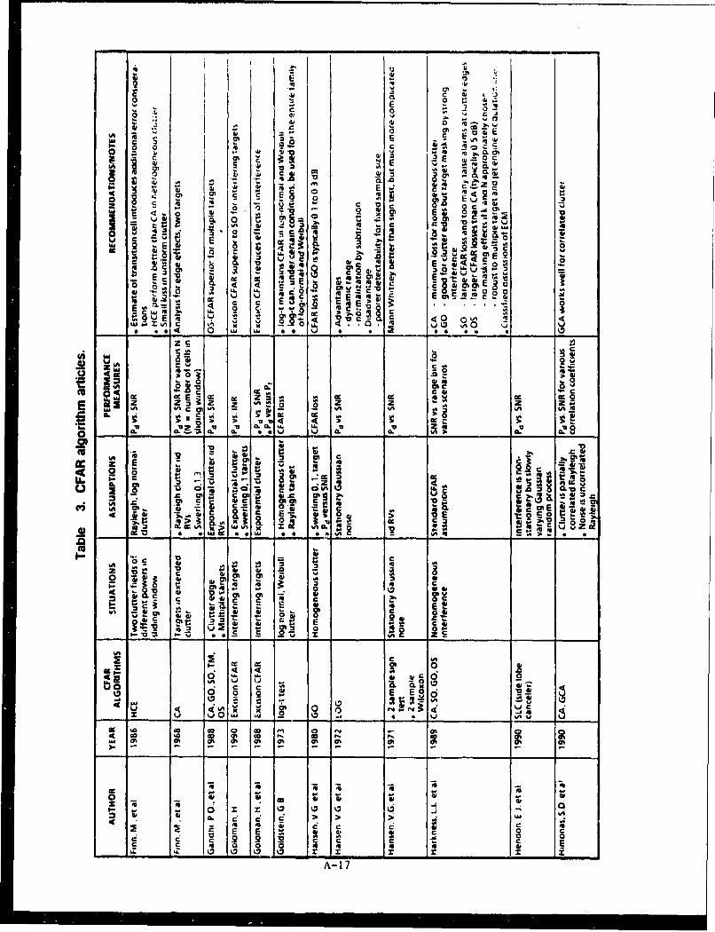
- . . I - . S
41 Z Ewl 41
0 0
c c
C. co I CL.
-~C atAC40 3 1 4 C
4A 4 T
- -c m C' atO3~
C 41 -. . R
2 c... V1t&A 41. cr E 2
10 A 's 400 40 4 U.4. 40 E .0 w wn G t
cc C.E -
cc- 4.
44
" "I ce C9z z = z zZ0i VI -vi
CL a. C
41 U4 1 2 2
C~0 C" CIM -
c 2 2m c 2 Cor61 .CA 441 C= gg h E z
>- '" - GDx "2 2 -a 6U W~ a- 4. L" - 2;
- 2
dc .C2 03 cedt 5~ 1~ 5-
4141 ~ ~ Og 8g 21 at E C
CA
1- 2 Q 0
891 .2
o~ L78~
4~I 0 4Oo @ . - .
oo f, 414 1 .9ti
0 0- co 4
Cc c C
Ac IM 4 0 1c,ID 0 0 ýd %)
S* z 41 4 C. 00 E
A-1 7

00
0C C C
0001 412
I-4 E..1N- 40
Co Go C41l v 1
00 a,4m JA 0 0
0 E0
-I - Ean C
IA 0 j
Ejju W C 41.
IL r. 'a 4A Cc
4& L41 ZiU4 .u'
0 e IT1 a-e
*o r. 2- V
V- E..1'o 6
06 Ic' 0c E CI
C - em~o ~49 3 5 .'aC _L a, E 2 CL j
Is~ 0. 3: 2O o. EOc = cE~U to ý t" C . C
0 0 fe.- 0-
z~~4 c 1c 1 .
w0 0 apCAE7 x - A.20: 13 2. 0 304
.5 D*1- r z 4 1~ =' z E m
IA -6a~~0 t~CE
~. C0 E. o ~o ~ C4a
40
vi kA V,-j44A >C 44 0.0 41u 4410
* 0 Ch f p _
10 I- 0 s
0 0 0
t IA x i z 2
4 -' - CC C 0A0118
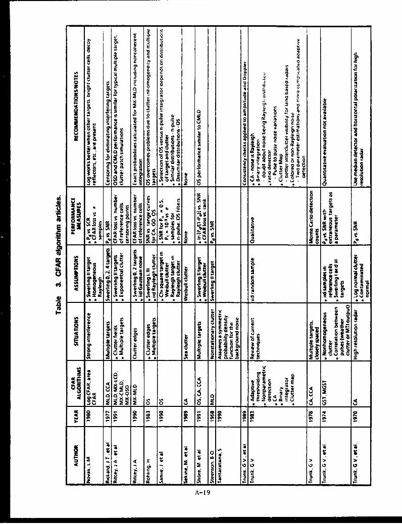
01 0
00 -
0. 00 t
If r, a c 0. E 0LD E - - 0
MA w w GD0 -D07. 3 %A0 C
GD - 0, Uc
2 CU-~ 7D- '0 73 3Cc L, cm CL CA, o 4-00~GD 00AG 01w 0. 0) IV Cr- C0. 91 CL GD mA l 3~G0 ' 0~ Z C 3~ 0. Q~ ~ ~ ,aD~0.G~E G
42 .2 A ~
132 E0) .k i -, &A -IC00 0. .D c2 ýssas 420. QI~0 9 =-;.1Icm 0 2mc # CC- I40 c j EGD E4S. cc U
*U **L .sb1GDz CCatD~GD -GO CL CL IIE --~ cI 0 Me.-t.. 1 2 Ca !f 4
t: 4/0 Se SO 6 0 oi -0 0lo lo' 0 S.4 GD cc ~~GD r.G 0 u m a I c
0U 0~ re. lz! -e c A 1- 0E6U ~U'1 - -A '19

- 0
AII C
06
to
F 0. C0. 0
0 -0
wD c
C z
IL S cc 1
GD wIc
U.L --t, E 6
C4 4A c 'cucc GDf(2 1 . I*Lma o.
wz 0 C E 0w
c 0 % U
E . -r . 0 Ze 2 a a.
cA h: c
o E E~ In- 3WE og' 01G %Au
0 0 6 GD GD Z
2 &SG C D~ 'oG
= -a 00' G^
- a ' a' a ~ a.~SdE fil koa0 '
a-L -4 a
cal cc Go~~~c 01DGD O D D G
I -~ - 5
S.. ~ ~ ~ 4 GD GcGmD ~ 31r r X . a
GUS. GOVERNMENT PRINTING OFFICE. 199 3-710-093-60 309 A-20
MISSION
OF
ROME LABORATORY
Rome Laboratory plans and executes an interdisciplinary program in re-
search, development, test, and technology transition in support of Air
Force Command, Control, Communications and Intelligence (C3 1) activities
for all Air Force platforms. It also executes selected acquisition programs
in several areas of expertise. Technical and engineering support within
areas of competence is provided to ESD Program Offices (POs) and other
ESD elements to perform effective acquisition of C3 1 systems. In addition,
Rome Laboratory's technology supports other AFSC Product Divisions, the
Air Force user community, and other DOD and non-DOD agencies. Rome
Laboratory maintains technical competence and research programs in areas
including, but not limited to, communications, command and control, battle
management, intelligence information processing, computational sciences
and software producibility, wide area surveillance/sensors, signal proces-
sing, solid state sciences, photonics, electromagnetic technology, super-
conductivity, and electronic reliability/maintainability and testability.