INTELLIGENT SPECTRUM HANDOFF VIA DOCITIVE … · teacher-based transfer learning scheme is used to...
87
INTELLIGENT SPECTRUM HANDOFF VIA DOCITIVE LEARNING IN COGNITIVE RADIO NETWORKS (CRNs) THE UNIVERSITY OF ALABAMA MARCH 2017 FINAL TECHNICAL REPORT APPROVED FOR PUBLIC RELEASE; DISTRIBUTION UNLIMITED STINFO COPY AIR FORCE RESEARCH LABORATORY INFORMATION DIRECTORATE AFRL-RI-RS-TR-2017-065 UNITED STATES AIR FORCE ROME, NY 13441 AIR FORCE MATERIEL COMMAND
-
Upload
trannguyet -
Category
Documents
-
view
215 -
download
0
Transcript of INTELLIGENT SPECTRUM HANDOFF VIA DOCITIVE … · teacher-based transfer learning scheme is used to...
INTELLIGENT SPECTRUM HANDOFF VIA DOCITIVE LEARNING IN COGNITIVE RADIO NETWORKS (CRNs)
THE UNIVERSITY OF ALABAMA
MARCH 2017
FINAL TECHNICAL REPORT
APPROVED FOR PUBLIC RELEASE; DISTRIBUTION UNLIMITED
STINFO COPY
AIR FORCE RESEARCH LABORATORY INFORMATION DIRECTORATE
AFRL-RI-RS-TR-2017-065
UNITED STATES AIR FORCE ROME, NY 13441 AIR FORCE MATERIEL COMMAND
NOTICE AND SIGNATURE PAGE
Using Government drawings, specifications, or other data included in this document for any purpose other than Government procurement does not in any way obligate the U.S. Government. The fact that the Government formulated or supplied the drawings, specifications, or other data does not license the holder or any other person or corporation; or convey any rights or permission to manufacture, use, or sell any patented invention that may relate to them.
This report is the result of contracted fundamental research deemed exempt from public affairs security and policy review in accordance with SAF/AQR memorandum dated 10 Dec 08 and AFRL/CA policy clarification memorandum dated 16 Jan 09. This report is available to the general public, including foreign nationals. Copies may be obtained from the Defense Technical Information Center (DTIC) (http://www.dtic.mil).
AFRL-RI-RS-TR-2017-065 HAS BEEN REVIEWED AND IS APPROVED FOR PUBLICATION IN ACCORDANCE WITH ASSIGNED DISTRIBUTION STATEMENT.
FOR THE CHIEF ENGINEER:
/ S / STEPHEN REICHHART Work Unit Manager
/ S / JOHN D. MATYJAS Technical Advisor, Computing & Communications Division Information Directorate
This report is published in the interest of scientific and technical information exchange, and its publication does not constitute the Government’s approval or disapproval of its ideas or findings.

REPORT DOCUMENTATION PAGE Form Approved OMB No. 0704-0188
The public reporting burden for this collection of information is estimated to average 1 hour per response, including the time for reviewing instructions, searching existing data sources, gathering and maintaining the data needed, and completing and reviewing the collection of information. Send comments regarding this burden estimate or any other aspect of this collection of information, including suggestions for reducing this burden, to Department of Defense, Washington Headquarters Services, Directorate for Information Operations and Reports (0704-0188), 1215 Jefferson Davis Highway, Suite 1204, Arlington, VA 22202-4302. Respondents should be aware that notwithstanding any other provision of law, no person shall be subject to any penalty for failing to comply with a collection of information if it does not display a currently valid OMB control number. PLEASE DO NOT RETURN YOUR FORM TO THE ABOVE ADDRESS. 1. REPORT DATE (DD-MM-YYYY)
MARCH 2017 2. REPORT TYPE
FINAL TECHNICAL REPORT 3. DATES COVERED (From - To)
DEC 2012 – SEP 2016 4. TITLE AND SUBTITLE
Intelligent Spectrum Handoff via Docitive Learning in Cognitive Radio Networks (CRNs)
5a. CONTRACT NUMBER N/A
5b. GRANT NUMBER FA8750-13-1-0046
5c. PROGRAM ELEMENT NUMBER 62788F
6. AUTHOR(S)
Fei Hu and Sunil Kumar
5d. PROJECT NUMBER T2CD
5e. TASK NUMBER AL
5f. WORK UNIT NUMBER AB
7. PERFORMING ORGANIZATION NAME(S) AND ADDRESS(ES)University of Alabama at Tuscaloosa Sponsored Research Office 601 University Blvd Tuscaloosa, AL 35486
8. PERFORMING ORGANIZATIONREPORT NUMBER
9. SPONSORING/MONITORING AGENCY NAME(S) AND ADDRESS(ES)
Air Force Research Laboratory/RITF 525 Brooks Road Rome NY 13441-4505
10. SPONSOR/MONITOR'S ACRONYM(S)
AFRL/RI 11. SPONSOR/MONITOR’S REPORT NUMBER
AFRL-RI-RS-TR-2017-065 12. DISTRIBUTION AVAILABILITY STATEMENTApproved for Public Release; Distribution Unlimited. This report is the result of contracted fundamental research deemed exempt from public affairs security and policy review in accordance with SAF/AQR memorandum dated 10 Dec 08 and AFRL/CA policy clarification memorandum dated 16 Jan 09. 13. SUPPLEMENTARY NOTES
14. ABSTRACTIn this project, we target the design of a Docitive Learning (also called transfer learning) based spectrum handoff design in Cognitive Radio Networks (CRNs). If the current channel quality is below a threshold, the secondary user (SU) should make one of the following decisions: (1) stay in the same channel and wait for it to become idle again (this strategy is called wait-and-stay), (2) stay in the same channel and adjust the channel parameters according to the varying channel conditions (this strategy is called stay-and-adjust), or (3) switch to another idle channel that meets its QoS requirement (this is the conventional spectrum handoff). In this project, we have applied a critic-based transfer learning model to implement an intelligent spectrum handoff with both node-to-node learning and self-learning. Additionally, a multi-teacher-based transfer learning scheme is used to learn handoff parameters from multiple neighbors. We have also built a comprehensive CRN testbed for spectrum handoff test. Such a testbed has other essential CRN components, such as spectrum sensing, mining and handoff. 15. SUBJECT TERMSCognitive Radio Networks (CRNs), Spectrum Handoff, Machine Learning
16. SECURITY CLASSIFICATION OF: 17. LIMITATION OF ABSTRACT
UU
18. NUMBEROF PAGES
19a. NAME OF RESPONSIBLE PERSON STEPHEN REICHHART
a. REPORT U
b. ABSTRACT U
c. THIS PAGEU
19b. TELEPHONE NUMBER (Include area code) N/A
Standard Form 298 (Rev. 8-98) Prescribed by ANSI Std. Z39.18
87

i
TABLE OF CONTENTS Section Page
List of Figures …………………………………………………………………….…..…...… iv
List of Tables ………………………………………………………………….……..….…... vi
List of Algorithms ……………………………………………………………………..……. vii
1.0 SUMMARY …………………………………………………….……………………... 1
2.0 INTRODUCTION ………………….……………………….…………….…...…...… 2
2.1 Significance of Establishing a Comprehensive CRN Testbed ………………….…..…..2
2.2 Transfer Actor-Critic Learning (TACT) Based Handoff Control ……………….…..…3
2.3 Multi-Teacher-Based Transfer Learning for Handoff Control ………………..……..…5
3.0 METHODS, ASSUMPTIONS, AND PROCEDURES ……………………………..….7
3.1 Cognitive Radio Network (CRN) Hardware Testbed …………………………..……... 7
3.1.1 Related Work …………………………………………………………………….…...... 7
3.1.2 Spectrum Sensing: Compressive Cyclostationary Sampling …………………………. 8
3.1.3 Spectrum Mining: Machine Learning Based Approach …………………………….. 10
3.1.4 Spectrum handoff: Markov Decision Based Handoff Control ………………………. 13
3.1.5 Rateless Codes for Throughput Improvement ………………………………………. 16
3.2 Intelligent Spectrum Management based on Transfer Actor-Critic Learning (TACT)....17
3.2.1 Related Work …………………………………………………………………………. 17
3.2.2 TACT-based Spectrum Mobility Management …………………………………….…. 18
3.2.2.1 Channel Selection Metric ……………………………………………………………... 18
3.2.2.2 Channel Utilization Factor (CUF) …………………………………………………….18
3.2.2.3 PU/SU NPRP M/G/1 Queueing Model ………………………………………………. 18
3.2.2.4 CDF-Enhanced Throughput …………………………………………………………...19
3.2.2.5 Q-Learning Based iSM ………………………………………………………………. 19
3.2.2.6 TACT-Based iSM ……………………………………………………………………..21
3.2.3 Channel Utilization Determination ……………………………………………………25
3.2.4 Throughput Determination in Decoding-CDF based Rateless Transmissions ……..……………26
3.2.5 CDF-Enhanced Fountain Codes …………………………………………………………………28
3.3 Multi-Teacher Learning for Optimal Spectrum Handoff ………………………………………..30
3.3.1 Related Work …………………………………………………………………………………….30

ii
3.3.2 Network Model …………………………………………………………………….... 31
3.3.3 Variables and Concepts ……………………………………………………………….32
3.3.4 Discretion Rule ………………………………………………………………………. 34
3.3.5 Residence Time and Completion Time ……………………………………………….34
3.3.6 Analysis of Expected Handoff Delay …………………………………………………36
3.3.7 Analysis of Expected Delivery Time ………………………………………………….39
3.3.8 Multi-Teacher Transfer Learning for Handoff Control ………………………………………….40
3.3.8.1 QoE-Driven, RL-based Spectrum Handoff. ……………………………………………………..40
3.3.8.2 Multi-Teacher Knowledge Transfer for Intelligent Spectrum Handoff. ………………………...40
4.0 RESULTS AND DISCUSSIONS ……………………………………………………………….44
4.1 USRP-Based CRN Platform Implementation……………………………………………………44
4.1.1 Testing of Spectrum Sensing. …………………………………...…………………………….…44
4.1.2 Testing of Spectrum Mining ………………….…………………….………………………….…47
4.1.3 Testing of Spectrum Handoff…………………………………………………………………….50
4.1.4 Testing of Raptor Codes……………………………………………………………….…………52
4.1.5 Other Test Results ………………………………………………………………………………53
4.2 TACT-based Spectrum Handoff: Performance Evaluation …………………………….……….54
4.2.1 Channel Selection………………………………………………………………………………..54
4.2.2 Average Queuing Delay…………………………………………………………………………57
4.2.3 Decoding CDF learning………………………………………………………..………………..58
4.2.4 Effect of Traffic Load on PER and PSNR………………………………………………………59
4.2.5 TACT-enhanced Spectrum handoff……………………………………………………………..61
4.3 Multi-Teacher Based Spectrum Handoff: Experimental Results ……………………………….64
4.3.1 QoS-aware Spectrum Handoff Scheme………………………………………………………….64
4.3.2 QoE-driven Spectrum Handoff Scheme…………………………………………………………66
4.3.3 MAL-based Spectrum Handoff Scheme…………………………………………………………69
5.0 CONCLUSIONS ……..…………………………..……….………………………….….. 72
REFERENCES ……………………………………………..…………..……………..…..… 73
LIST OF SYMBOLS, ABBREVIATIONS, AND ACRONYMS ……………………………77
iii
LIST OF FIGURES Figure Page
1 The Big Picture of Intelligent Spectrum Management (iSM) Concept ..………….…. 5
2 Compressive Cyclostationary Spectrum Sensing …………………………….……..10
3 (a) Conventional HMM with Finite States; (b) HDP-HMM ……………………..…12
4 Synthetic Data: Channel State Transitions …………………………………………..13
5 Transfer Learning Based Spectrum Handoff ………………………………………...14
6 Software Framework: Raptor Codes for Video Transmission Over CRN…………...16
7 Q-Learning Based iSM …………………………………………………………….21
8 Gephi-Simulated Expert SU Searching …………………………………………..… 22
9 TACT Based SU-to-SU Teaching ………………………………………………….. 24
10 Frame Transmission Pattern …………………………………………………………26
11 Benefits of Using CDF: (left) No CDF Case; (right) Using CDF ………………….. 28
12 Prioritized Fountain Codes …………………………………………………………..29
13 Hybrid PRP/NPRP M/G/1 Queueing Model.……………………………………..….32
14 Concept of Delay Cycle………………………………………………………………32
15 Relationship Among the Random Variables During the Transmission Service …….34
16 Three Types of Delay Cycles for Switching Case …………………………………...37
17 The Delay Cycle for Staying Case ………………………………………...………....39
18 Information Geometry Based Node-to-Node Teaching ……………………….….…41
19 Multi-Teacher Based Spectrum Handoff……………………………………………..42
20 USRP N210 and GNU Radio Control GUI .……………………………………….…44
21 Testbed Node Components …………………………………………………………..45
22 CSP Detector Software Implementation …………………………………………… 45
23 Spectrum Sensing Results …………………………………………………………...46
24 Cyclic Features for Different Signals ……………………….…………………….…47
25 Performance Comparison of Different Detection Schemes …………………………48
26 Spectrum Classification Performance ………………………………………………..48
27 SVM-Based Pattern Clustering for Non-cyclic Domain …………………………….49
28 SVM-Based Pattern Clustering for Compressive Cyclic Domain ……………….......49

iv
29 Setup of Spectrum Handoff Test ……………………………………………..…….. 50
30 Multi-thread GNU Radio Programming …………………………………………….51
31 Video quality (Before/After Spectrum Handoff)…………………………………… 52
32 One Frame of the Received Video. (Left) Video Transmission without Raptor Codes;
(Right) Video Transmission with Raptor codes.……………………………………. 52
33 TDMA-based Video Communications ……………………………………………....53
34 Multi-video Transmission Test………………………………………………………54
35 Channel Selection Performance…..….………………………………………………55
36 Comparison of Different Channel Selection Schemes (I)…………………………56
37 Comparison of Different Channel Selection Schemes (I)…………………………57
38 Average Delay for NPRP Queueing Model and Non-prioritized Model……………..57
39 Estimated CDF for Different SNR Levels ………………………………………….58
40 Throughput of Different Rateless Coding Schemes ……………………………….. 58
41 Zoomed-in Section of Details in Figure 40 ………………………………………….59
42 The Effects of Traffic Load on Video PSNR ……………………………………….60
43 Video Effect Comparisons of Learning-based and Myopic Handoff Schemes ……...60
44 Learning Performance with TACT, Q-learning and Myopic Scheme ………………62
45 Performance Comparisons with and without Decoding CDF ……………..……..…63
46 Effects of Normalized PU Traffic Load on the Average Delivery Time ……………65
47 Effects of SU Arrival Rate on the Average Delivery Time ………………………...66
48 Effects of SU Service Time on the Average Delivery time ………………….….…67
49 Average PSNR (in SU1 and SU2) of Foreman Video Sequence ……………….…69
50 Comparison of RL-based and Our Proposed MAL-based Schemes ……….……….70
51 Visual Comparison (Frame 201) of Different Handoff Schemes …………………..71

v
LIST OF TABLES
Table Page
1 An Example of Channel Adaptation ………………………………………….…….27
2 Main Parameters Used in Queueing Analysis ……………………………………...33
3 Experiment Parameters in Compressive Spectrum Sensing ……………………….47
4 Experiment Parameters in Intelligent Spectrum Handoff (Sender Side) …….…….50
5 Experiment Parameters in Raptor Codes for Reliable Video Transmission ……….53
6 Parameters in Multi-video Transmissions ………………………………………….54
7 Simulation Parameters …………………………………………………………..…55
8 PER Comparison for Different Traffic Loads. …………………………………. ... 59
9 Simulation Parameters ………………………………………………………………68
10 Comparisons of Total Packet Error Rate for Different Normalized Loads……..…...68

vi
LIST OF ALGORITHMS
Algorithm Page
1 TACT-Based Spectrum Decision Scheme ………………………………….25
2 Decoding CDF Estimation ……………………………....………………….29
3 MAL-Based Spectrum Handoff Scheme. …………………………………43

Approved for Public Release; Distribution Unlimited. 1
1.0 SUMMARY
This project began on January 1, 2013, and ended on September 30, 2016. We have used the concept of docitive learning (also called transfer learning), to perform intelligent spectrum handoff in cognitive radio networks (CRNs). In particular we have achieved the following outcomes: First, we have built a comprehensive CRN testbed for spectrum handoff test. Such a testbed has other essential CRN components, such as spectrum sensing, mining and handoff. Second, we have applied a critic- based transfer learning model to implement an intelligent spectrum handoff with both node-to-node learning and self-learning. Third, a multi-teacher-based transfer learning scheme is used to learn handoff parameters from multiple neighbors.
During this project, we have delivered the following products: • Three IEEE journal papers (published or accepted for publishing).• One international conference paper.• Hardware demos on learning-based cognitive radio networks.
More details of the above deliverables are given below:
(1) Journal Papers (published or accepted):
[1] Yeqing Wu, Fei Hu, Sunil Kumar, ”Apprenticeship Learning based Spectrum Decision in Multi-Channel Wireless Mesh Networks with Multi-Beam Antennas,” IEEE Trans. Mobile Computing, vol. 16, no. 2, pp. 314-325, Feb. 1 2017.
[2] Yeqing Wu, Fei Hu, Sunil Kumar, and Yingying Zhu, ”Multi-Teacher Knowledge Transfer for Optimal CRN Spectrum Handoff Control with Hybrid Priority Queueing”, IEEE Trans. Vehicular Technology, to appear, 2017.
[3] Xin-lin Huang, Fei Hu, Jun Wu, et. al., ”Intelligent Cooperative Spectrum Sensing via Hierarchical Dirichlet Process in Cognitive Radio Networks,” IEEE J. Selected Areas in Communications (JSAC), vol. 33, no. 5, pp. 771-787, May 2015.
(2) Conference Paper:
[1] Ji Qi, Fei Hu, Xin Li, Koushik A. M, Lei Hu, And Sunil Kumar, “CR-Based Video Communication Testbed with Robust Spectrum Sensing / Handoff,” 13th International Conference on Information Technology: New Generations, Las Vegas, Apr 2016.
(3) Hardware Demos:
We have also built hardware demos on teaching-and-learning based spectrum handoff scheme.

Approved for Public Release; Distribution Unlimited. 2
2.0 INTRODUCTION
2.1 Significance of Establishing a Comprehensive CRN Testbed
CRNs have been investigated extensively for over one decade [1]. Most of those CRN studies are based on pure theoretical analysis and simulation validations. There is a strong need for building a hardware-based CRN testbed for two reasons: First, there may exist big differences between theoretical assumptions and practical scenarios. For example, many CRN channel allocation schemes assume that the unoccupied channels can be detected in real-time within a wideband (from a few hundred MHz to a few GHz). But today’s commercial CRN products have only one or two transceivers to sense the narrow bands (a few hundred MHz in each band) with noticeable sensing delay (>2ms). Second, a comprehensive hardware testbed can integrate main CRN elements, including spectrum sensing, channel allocation, network protocols, etc., and provides a realistic research environment. Many CRN routing protocols [2] simply assume that the route discovery process becomes stable once the channel assignment is finished in each link (via graph coloring or other algorithms). However, the effect of spectrum handoff must be considered in some links from time to time when the channel conditions change. Additionally, spectrum handoff does not necessarily mean actual channel switching in a link. Sometimes we do not need to switch the channel if the primary user (PU) will release the channel quickly. Since the channel switching can take certain time, including the time for band sensing, transceiver switching, data buffering, etc., in some cases the stay-and-wait scheme (i.e. waiting for the channel to become available again without switching to another channel) can be a better spectrum handoff policy.
Some hardware-based CRN testbeds have been described in [3,4]. However, those testbeds have the following drawbacks:
(1) Lack of fast spectrum sensing: Most of those hardware testbeds use energy detection methods to detect unused spectrum. Such a method has inaccurate spectrum sensing due to the difficulty of distinguishing PU signals and network noise.
(2) Lack of spectrum mining functions: There are rich patterns among the detected spectrum. For instance, some spectrum bands have higher probability of being unoccupied than other bands. We can classify the bands based on their signal-to-noise ratios (SNRs). And there could exist strong correlation between spectrum occupancy and geographical locations. These spectrum patterns can be very helpful in wireless applications. For example, we can assign the stable (i.e. unoccupied), high-quality channels to higher priority users. Unfortunately, existing CRN testbeds do not support the spectrum mining (i.e. spectrum pattern recognition and analysis).
(3) Lack of intelligent spectrum handoff control: Spectrum handoff is a critical operation in CRNs. A secondary user (SU) needs to vacate the channel and switch to another one when the PU occupies the channel. However, channel switching takes certain time (>2ms). And sometimes the PU just uses the channel shortly and then immediately releases it. Therefore, a spectrum handoff scheme needs to make a smart decision between actual channel switching and stay-and-wait scheme.
Novelty of Our Design: So far we are not aware of any systematic CRN platforms built so far, except for some general multi-hop wireless platforms such as [3], or 802.11-like wireless testbeds such as [4]. In this project, we have built a novel CRN testbed, which has the following four features:
• Compressive cyclostationary spectrum sensing: To achieve a fast and accurate spectrum sensing, weuse compressive sensing theory to reduce the spectrum samples to be sensed and analyzed. Thecyclostationary domain features can better identify the signal patterns than conventional energy-detection-based spectrum sensing scheme.
• Machine learning based spectrum mining: To further extract the intrinsic features of spectrum

Approved for Public Release; Distribution Unlimited. 3
signals, we propose to use machine learning algorithms to form the clusters of spectrum signals, and identify the spectrum changing trends.
• Optimized spectrum handoff : Conventional spectrum handoff schemes aim to optimize the short-term throughput without considering the impact of the current handoff decision on the long-termthroughput. Moreover, they do not distinguish between actual channel switching and stay-and-waitschemes.
• Support of high-throughput communications: To enhance the throughput of CRNs, we propose to useRaptor codes to support real-time multimedia communications over CRNs. By assigning moresymbols to good channels, we can improve the quality of experience (QoE) of video traffic.Our testbed is built on a powerful software defined radio (SDR) device - USRP N210. We have
implemented spectrum sensing, spectrum mining, spectrum handoff, TDMA scheduling, rateless codes, and other CRN functions. We have used both Python and C++ to build the software in GNU Radio environment. This CRN testbed can serve as the basis for advanced CRN protocol implementation. Many different spectrum measurements can be performed in the testbed.
In Section 3.1 we will describe the CRN platform implementation details.
2.2 Transfer Actor-Critic Learning (TACT) Based Handoff Control
The spectrum mobility, conventionally called spectrum handoff, is a critical issue in CRNs due to the dynamic channels [5]. Although a SU does not know exactly when the PU will reoccupy the channel, it wishes to have a smooth spectrum usage (i.e. less spectrum handoffs), in order to support its QoS requirements. In this research, we target an intelligent spectrum mobility (iSM) design. If the current channel quality (which can be estimated based on the PER, channel throughput and PDR) is below a threshold, the SU should make one of the following decisions: (1) stay in the same channel and wait for it to become idle again (this strategy is called wait-and-stay), (2) stay in the same channel and adjust the channel parameters according to the varying channel conditions (this strategy is called stay-and-adjust), or (3) switch to another idle channel that meets its QoS requirement (this is the conventional spectrum handoff) [6].
To manage the spectrum decisions smoothly, first we define a suitable channel quality metric so that a spectrum handoff policy knows which channel to switch to. Particularly, we define a proper Channel Selection Metric (CSM) that accurately reflects the quality of a channel based on three important factors in rateless CRN transmissions:
CUF: A SU cares not only about the channel occupancy status (idle or busy), but also the channel holding time (CHT) [7]. In this work, we determine CUF by considering the spectrum sensing accuracy, false alarm rate, and CHT [7].
PDR: In CRNs, many SUs may contend for the channel access, the new SU will stay in the queue until all the existing SUs (arrived earlier) and the PUs (arrived at any time) are served. We analyze this condition using non-preemptive M/G/1 queueing model to determine the expected waiting delay for a SU in the queue. This delay determines the PDR associated with a channel. The SU should select a channel with a PDR which is less than the preset threshold.
Flow Throughput: This parameter is determined by a rateless transmission model in Rayleigh fading channel, under time-varying channel conditions. We use the state-of-the-art algorithm, decoding-CDF [8], along with our invented special type of rateless codes, called Prioritized Raptor codes (PRC) [9], to determine the flow throughput and perform the spectrum adaptation process. With decoding-CDF, the SU can determine the number of packets to be sent to maintain the stable QoS. To the best of our knowledge, we are the first team to employ rateless codes with decoding-CDF to achieve a cognitive link adaptation in CRNs.
Additionally, the spectrum decision should maximize the performance for the entire communication

Approved for Public Release; Distribution Unlimited. 4
session instead of just maximizing the performance for a short term. We achieve iSM by integrating the CSM with the machine learning algorithms. Spectrum handoff strategy based on long-term optimization model, such as Q-learning used in our previous work [6], can achieve high-throughput multimedia transmissions over CRN links. The Q-learning can determine the proper spectrum decision actions based on the SU state estimation (including PER, queuing delay, etc.). However, in the beginning the SU has no prior knowledge of the CRN environment. It starts with a trial-and-error process, explores each action in every state, and achieves optimal state after some iterations. Thus Q-learning could take considerable time to converge to an optimal stable solution [10]. When more states and actions are defined, the learning process could be considerably prolonged.
To enhance the spectrum decision learning process, we focus on the transfer learning methods in which a new SU uses the already mature policies of the existing ‘expert’ SUs that have an efficient channel adaptation process. Unlike general learning models (such as Q-learning) that ask a SU to adapt to its own radio environment [10], [11], the transfer learning utilizes other nodes’ knowledge to enhance the existing node’s performance.
The TACT method is a special Docitive learning [34] scheme, and uses a combination of actor-only and critic-only models [12]. While the actor performs the continuous actions without the need of optimized value function, the critic criticizes the actions taken by the actor and keeps updating the value function. By using TACT, a new SU does not need to perform iterative optimization algorithms from scratch which could take a long time to converge to a stable solution. To enhance the accuracy of transferring the optimal policy from the expert SU to a new SU, we enhance the original TACT algorithm by exploiting the temporal and spatial correlations in the SU’s traffic profile, and update the value function and the policy function separately for easy knowledge transfer.
To form a complete TACT-based transfer learning framework, we solve the following two important issues: 1) Who should be the expert SU? The SU should find an appropriate expert node that has performed similar communication tasks. For instance, if a new SU (called ‘actor’) is transmitting video data, it should hunt for an expert SU with similar video QoS and QoE demands. We will use manifold learning algorithms to find a suitable expert SU. 2) How to transfer? An efficient knowledge transfer model is used to transfer the handoff policies from the expert node to a student node. An SU learns from an expert SU in the beginning of the TACT algorithm, and then gradually starts learning by itself. This is very similar to the teacher-student model in the human world.
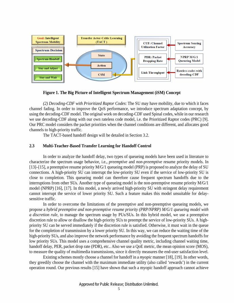
By integrating Rateless codes based decoding-CDF with the TACT-based transfer learning method, we can enhance the throughput of the system within the available CHT by making use of the SU’s past transmission profile as well as its neighboring expert SU’s knowledge. The CSM concept as well as the big picture of our iSM model is shown in Figure 1.
The main contributions of our TACT-based handoff control are twofold: (1) Teaching-based Spectrum Decision: Previously we have used the transfer learning algorithms
(such as apprenticeship learning) in the field of machine learning for CRNs. However, our previous node-to-node ‘teaching’ algorithms still have some areas to be improved. For example, we should avoid the exact imitation of the expert node’s policy since each node in the network may experience different channel conditions. Therefore, it is necessary to consider a transfer learning algorithm which can use the learned policy from the expert SU to build its own optimized learning model, by fine-tuning the expert policy according to the channel conditions it experiences. In this regard, we go for the state-of-the-art TACT algorithm [28], where the new SU receives the learned policy from the expert SU and uses it to build its own policy without having to explore each action in every state. More importantly, we connect the Q-learning scheme with TACT model, to receive the handoff policy from the expert node. This greatly enhances the node-to-node ‘teaching’ process without introducing much overhead on the expert node.
Approved for Public Release; Distribution Unlimited. 5
Figure 1. The Big Picture of Intelligent Spectrum Management (iSM) Concept
(2) Decoding-CDF with Prioritized Raptor Codes: The SU may have mobility, due to which it faces channel fading. In order to improve the QoS performance, we introduce spectrum adaptation concept, by using the decoding-CDF model. The original work on decoding-CDF used Spinal codes, while in our research we use decoding-CDF along with our own rateless code model, i.e. the Prioritized Raptor codes (PRC) [9]. Our PRC model considers the packet priorities when the channel conditions are different, and allocates good channels to high-priority traffic.
The TACT-based handoff design will be detailed in Section 3.2.
2.3 Multi-Teacher-Based Transfer Learning for Handoff Control
In order to analyze the handoff delay, two types of queueing models have been used in literature to characterize the spectrum usage behavior, i.e., preemptive and non-preemptive resume priority models. In [13]–[15], a preemptive resume priority M/G/1 queueing model (PRP) is proposed to analyze the delay of SU connections. A high-priority SU can interrupt the low-priority SU even if the service of low-priority SU is close to completion. This queueing model can therefore cause frequent spectrum handoffs due to the interruptions from other SUs. Another type of queueing model is the non-preemptive resume priority M/G/1 model (NPRP) [16], [17]. In this model, a newly arrived high-priority SU with stringent delay requirement cannot interrupt the service of lower priority SU. Such a feature makes this model unsuitable for delay-sensitive traffic.
In order to overcome the limitations of the preemptive and non-preemptive queueing models, we propose a hybrid preemptive and non-preemptive resume priority (PRP/NPRP) M/G/1 queueing model with a discretion rule, to manage the spectrum usage by PUs/SUs. In this hybrid model, we use a preemptive discretion rule to allow or disallow the high-priority SUs to preempt the service of low-priority SUs. A high-priority SU can be served immediately if the discretion rule is satisfied. Otherwise, it must wait in the queue for the completion of transmission by a lower priority SU. In this way, we can reduce the waiting time of the high-priority SUs, and also improve the network performance by avoiding the frequent spectrum handoffs for low priority SUs. This model uses a comprehensive channel quality metric, including channel waiting time, handoff delay, PER, packet drop rate (PDR), etc.. Also we use a QoE metric, the mean opinion score (MOS), to measure the quality of multimedia transmissions, since it directly measures the end-user satisfaction level.
Existing schemes mostly choose a channel for handoff in a myopic manner [18], [19]. In other words, they greedily choose the channel with the maximum immediate utility (also called ‘rewards’) in the current operation round. Our previous results [15] have shown that such a myopic handoff approach cannot achieve

Approved for Public Release; Distribution Unlimited. 6
the optimal long-term rewards. Reinforcement learning (RL) may be used to achieve the optimal long-term reward. However, the convergence of the learning process in RL-based spectrum handoff is usually slow due to the varying and complex communication conditions in CRNs. In [20], we have introduced the concept of apprenticeship learning (AL) to enhance the SU’s learning process. It enables an SU (known as a student or apprentice) to learn transmission policies from the experienced users (known as teachers or experts).
To avoid poor selections of the teachers, we use the manifold learning to select multiple teachers who have useful transmission “skills”. For example, they may know how to select a suitable initial Markov state and use the appropriate state transmission matrix. The knowledge from these teachers is used to guide the handoff behavior of the student SU.
The main contributions of our work are two-fold: (1) Hybrid PRP/NPRP M/G/1 queueing model with discretion rule for spectrum handoff that supports
differentiated services. Our previous work used the non-preemptive queueing model [15], [20]. This work significantly improves it by using hybrid queueing model, in which high-priority SUs are allowed to preempt the service of low-priority SUs based on a discretion rule. It can avoid frequent spectrum handoffs for the low-priority SUs, meanwhile, reducing unnecessary waiting time for the high-priority SUs. Although our hybrid queueing model more accurately reflects the PU/SU traffic transmission relationship, it is challenging to mathematically analyze the queueing delay. We introduce the concept of delay cycle, and utilize Laplace transform of time functions to develop the closed-form handoff delay results.
(2) Multi-teacher apprenticeship learning for QoE-driven spectrum handoff. In RL-based spectrum handoff, when an SU enters the CRN, it could take a long time to make an optimal spectrum decision due to the difficult choice of initial RL parameters and utility function for the complex radio conditions. We propose a multi-teacher apprenticeship learning (MAL) framework to speed up the learning process by enabling a newly joined SU to learn from multiple neighboring SUs. To search the suitable ‘teachers’, we use the manifold learning to find ‘teachers’ with statistically similar features to the ‘student’.
In Section 3.3 we will explain the MAL algorithms and implementation.
Approved for Public Release; Distribution Unlimited. 7
3.0 METHODS, ASSUMPTIONS, AND PROCEDURES
3.1 Cognitive Radio Network (CRN) Hardware Testbed
In this section, we describe our design methodology of a hardware testbed for the study of multimedia transmissions over CRNs. Our testbed is built on the recent Universal Software Radio Peripheral (USRP) hardware, and has the following three features: (1) Spectrum sensing: an essential function of CRNs is spectrum sensing. We propose to use compressive sensing to sample the wide bandwidth. Such a sub-Nyquist spectrum sampling greatly reduces the signal processing complexity. We then use cyclostationary domain features to detect the spectrum signals. (2) Spectrum mining: Learning spectrum features, such as 24/7 trends, is critical to proactive communications. To mine the patterns of the sensed bands, machine learning schemes are used to identify the important spectrum features. (3) Spectrum handoff: another essential function of CRNs is spectrum handoff. To adapt to various QoS requirements of multimedia applications, we propose a Markov decision based spectrum handoff control scheme that can switch channels at the approximate times. The developed CRN testbed can serve as a platform for testing CRN communication protocols in dynamic spectrum environment.
3.1.1 Related Work. Some basic CRN spectrum measurement methods have been proposed in [21] [22] [23]. However, they only focus on basic aspects of signal measurement in CRN systems, and do not aim to build a comprehensive CRN platform with major CRN functions, including spectrum sensing, spectrum handoff, and spectrum mining. A CRN testbed was built at Tennessee Technological University with simple spectrum sensing and
communication schemes [24]. It can scan the available spectrum, and has implemented a multi-hop routing protocol. However, its spectrum sensing operation is very slow when handling a few GHz of bandwidth. A smart-grid-oriented CRN testbed was built in [25] with real-time communication functions. Since it mainly targets the smart grid communication infrastructure, it does not have the essential CRN functions including spectrum handoff and management. An education-oriented CRN testbed was built in [26]. It does not have comprehensive spectrum sensing, mining and handoff functions since its main purpose is to show students the dynamic spectrum environment and some basic CRN protocols.
A large-scale CRN testbed was introduced in [27] with distributed spectrum sensing. Its sensing function is still based on the energy detection of PU’s signals. A hardware design of CRN testbed was introduced in [28], which covers the physical layer signaling techniques and FPGA-based spectrum sensing function. However, it does not discuss the details of software implementation for CRN spectrum management functions.
The USRP-based testbeds have been studied in some projects. For example, a USRP-based software radio platform was discussed in [29]. It has spectrum sensing function and some basic network security functions. Our work here focuses on the most important CRN functions, i.e. spectrum sensing, spectrum mining, and spectrum handoff, since other advanced CRN protocols are built on those three functions. Below we briefly review other related works on the implementation of those three functions. Compressive sensing has been used in CRN spectrum sensing to reduce the number of samples of the spectrum signals [30], [31]. However, it needs the signal reconstruction operation that uses the iterative optimization algorithms to recover the original spectrum map. Such a reconstruction can cause long computation delay and large energy consumption due to the complex optimization algorithms. Our work presented here overcomes such a drawback by avoiding the L1-norm reconstruction.
Moreover, we apply compressive sensing in the cyclostationary domain instead of time domain. It can accurately detect and even classify the PU signals in low-SNR links, thanks to its cyclic frequency features
Approved for Public Release; Distribution Unlimited. 8
that can be extracted and recognized from the modulated signals. Spectrum handoff is a critical function of CRNs since a channel can be reoccupied by the PUs at any time. Some researchers have investigated this issue. For example, some performance metrics are proposed in [32] to measure the handoff performance, such as the link availability probability, the number of spectrum handoff operations, channel switching delay, and link access failure probability. However, it does not consider the stay-and-wait handoff policy. In [33] the comparisons between reactive and proactive spectrum handoff schemes are made. However, the handoff protocol details are not provided. It is important to achieve an intelligent spectrum handoff since the complex, dynamic CRN radio conditions require an adaptive, self-learning channel switching strategy. Past handoff effects (in terms of the throughput and delay) can be used to determine the future handoff operations. In the work reported here, we have built an intelligent spectrum handoff scheme by using a node-to-node transfer learning model: A node can perform handoff by learning the radio environment by itself without interacting with its neighbors; A node can also accept the ‘teaching’ results from another node that already knows a good strategy to perform handoff. To the best of our knowledge, this is the first CRN testbed with intelligent spectrum sensing, mining, and handoff, built on USRP (hardware) and GNU Radio (software) platform. Our design emphasizes the essential CRN functions and provides convenient interfaces for future protocol extensions. CRN should be cognitive, and intelligent algorithms could play a critical role in the network control. 3.1.2 Spectrum Sensing: Compressive Cyclostationary Sampling. The requirements of spectrum
sensing include fast detection (< 1ms), high accuracy and low implementation complexity. Matched-filter-based sensing scheme requires the prior knowledge of the PU’s signals. Energy detector does not need such a prior knowledge, but it is not robust to radio shadowing and fading.
We are the first team to integrate compressing sensing principle and cyclostationary domain signal processing into a low- cost, high-accuracy spectrum sensing scheme. But our integration is not the simple combination of those two aspects. In fact, we significantly improve existing compressive sensing models by removing the signal reconstruction phase. In other words, we analyze the spectrum directly from the collected sparse spectrum signal samples without recovering the original complete spectrum map. This scheme can reduce the spectrum sensing delay and computation overhead. The motivation of integrating the above two aspects is as follows: Although cyclostationary detector has been proposed to improve the sensing accuracy, it has a prohibitively high computation cost since the detector needs to sense a wide band (from a few hundred MHz to several GHz). By using compressive-sensing-based algorithms, we just need to sample the spectrum bands at a sub-Nyquist rate. By applying the cyclostationary features in compressive signal processing (CSP), we can achieve fast, accurate spectrum detection. Below we will introduce the principles of cyclostationary detector and compressive sensing, followed by a description of our integrated spectrum sensing scheme. (1) Cyclostationary Detector Modulated signals typically involve sine wave carriers, regular pulse trains, repeating spreading codes, periodic hoping sequences, or cyclic prefixes, all of which have some sort of signal periodicity. Even though the data is a stationary random process, these modulated signals are characterized as cyclostationary, since their statistics exhibit certain periodicity. The periodicity can also be intentionally introduced into the signals such that a receiver can exploit it for parameter estimation. Cyclostationary domain can be used to analyze the features that are not stationary but with periodical patterns in specific frequencies. Generally, it can be calculated by Fourier transform (FT) of the

Approved for Public Release; Distribution Unlimited. 9
autocorrelation of non-stationary signals. In recent years, cyclostationary feature detector has been introduced as a two-dimensional signal processing method for the recognition of modulated signals in the presence of noise and interference.
Cyclostationary signal x(t) has the property as follows [34]:
𝑚𝑚𝑥𝑥(𝑡𝑡) = 𝑚𝑚𝑥𝑥(𝑡𝑡 + 𝑘𝑘𝑘𝑘) = 𝐸𝐸[𝑥𝑥(𝑡𝑡)] (𝑘𝑘 = 1,2, …𝑁𝑁) (1)
where m is the mean value of x(t), E is the expectation value of the signal mean, T is the cycle period. The signal autocorrelation is
𝑅𝑅𝑥𝑥(𝑡𝑡, 𝜏𝜏) = 𝑅𝑅𝑥𝑥(𝑡𝑡 + 𝑘𝑘𝑘𝑘, 𝜏𝜏) (𝑘𝑘 = 1,2, … ,𝑁𝑁) (2)
Taking FT, we can get the spectral correlation function (SCF). The sufficient statistics used for the detection are obtained through non-linear squaring operation. FFT-based methods can be used in digital implementation of the cyclostationary detectors. Given N samples divided into different blocks (TF F T samples each block), a simplified SCF is estimated as:
𝑆𝑆𝑥𝑥𝑎𝑎(𝑓𝑓) = 1𝑁𝑁𝑁𝑁∑ 𝑋𝑋𝑁𝑁𝑇𝑇𝑇𝑇𝑁𝑁𝑁𝑁𝑛𝑛=0 𝑛𝑛, 𝑓𝑓 + 𝑎𝑎
2 𝑋𝑋𝑁𝑁𝑇𝑇𝑇𝑇𝑁𝑁∗ (𝑛𝑛, 𝑓𝑓 − 𝑎𝑎
2) (3)
where XTF F T is the N-point FFT of SCF, and α is the bandwidth of each sample block.
(2) Compressive Measurement Design
In time domain, the received signal can be processed by compressive sensing (CS) to obtain a low-dimensional vector Y after using a sensing matrix Φ as follows [14]:
Y = ΦX (4)
where X is an M × 1 vector representing the Nyquist samples of x(t), Y is the N × 1 compressed measurement vector, and Φ is an N × M measurement matrix.
(3) Cyclostationary Compressive Spectrum Sensing
Because of the advantages of the cyclic features and compressive sensing, we propose the design of cyclostationary compressive measurement processing (CCMP) detector. It is an adaptive feedback system. The detector has a good balance between detection accuracy and cyclic rate, because both the sparsity and cyclostationary features of PUs’ signals are explored in the sensing step. The detection or classification is made directly on the measurements without signal reconstruction. Therefore, the sensing rate, time and energy consumption are reduced, meanwhile the detection accuracy and robustness to the noise are maintained.
As shown in the Figure 2, we add the cyclic features into the CS random measurements and build a sensing matrix, which is implemented via the low-rate sampling of the cyclic features that can be calculated through the filter banks. We utilize the adjustable filter banks to separate the wideband into different channels. Depending on the inter-channel frequency distance, we can set up a guard distance. When the distance of the measurements gets close to each other, the sensing rate increases and the bandwidth from the filter bands is reduced. Thus we can adaptively change the resolution of our cyclic spectrum measurement for different radio

Approved for Public Release; Distribution Unlimited. 10
environments and ensure a high accuracy for the detector. Note that the compressive spectrum samples will be directly used for the spectrum analysis without L1-norm based signal reconstruction. This is an important improvement over traditional compressive sensing schemes since we can significantly reduce the signal processing time by avoiding signal reconstruction.
Figure 2. Compressive Cyclostationary Spectrum Sensing 3.1.3 Spectrum Mining: Machine Learning Based Approach. Spectrum mining is a largely unexplored topic so far. It is an important aspect in CRNs due to the following two reasons: (1) The need for spectrum classification: The spectrum sensing function described above has limited use. It can only tell which channels are idle (i.e. not occupied by the PUs) as well as the signal quality in that channel. It will be very useful to classify the channels into different groups, based on the channel idle durations, idle times, signal quality, physical locations, etc. Among those channel groups we can select the channels with long idle durations and high signal quality, and assign them to the high-priority traffic flows. (2) The need for spectrum trend prediction: For some CRN operations, we need to predict the channel availability. For instance, to perform a low-delay spectrum handoff, it is helpful to predict which channel has the best quality and the longest idle duration in the next phase. In proactive routing protocol, it is necessary to know which good channels will be available in the next phase. In the previous section, we designed a compressive cyclostationary sensing mechanism for accurate, fast channel detection. We can directly use the sparse cyclostationary signal samples without L1-norm signal

Approved for Public Release; Distribution Unlimited. 11
reconstruction. Here, we further use machine learning algorithms to process those sparse samples to analyze the spectrum features. Particularly, we will use support vector machine (SVM) for spectrum clustering, i.e. classifying those channels into different groups based on their cyclostationary patterns.
(1) Spectrum Clustering
SVM [35] has accurate pattern classification capability. Given the input epoch x (the detected cyclostationary features of each channel), the optimization problem can be formulated as follows:
∑ ∑ (𝑟𝑟𝑗𝑗𝑗𝑗𝑗𝑗:𝑗𝑗≠𝑗𝑗𝑘𝑘𝑗𝑗=1𝑝𝑝(𝑥𝑥)
𝑚𝑚𝑗𝑗𝑛𝑛 𝑝𝑝𝑗𝑗(𝑥𝑥) − 𝑟𝑟𝑗𝑗𝑗𝑗𝑝𝑝𝑗𝑗(𝑥𝑥))2 𝑠𝑠. 𝑡𝑡.∑ 𝑝𝑝𝑗𝑗(𝑥𝑥) = 1𝑘𝑘𝑗𝑗=1 (5)
Here rij is the estimated pairwise class probabilities between pi(.) and pj (.), and pi(x) is a conditional probability:
𝑝𝑝𝑗𝑗(𝑋𝑋) = 𝑃𝑃(𝑦𝑦 = 𝑖𝑖|𝑥𝑥), (𝑖𝑖 = 1,2, … , 𝑘𝑘) (6)
Note that rij + rji = 1. We can re-write the above equation in a convenient form:
2𝑃𝑃𝑁𝑁(𝑥𝑥)𝑄𝑄𝑃𝑃(𝑥𝑥) = 12𝑃𝑃𝑁𝑁(𝑥𝑥)𝑄𝑄𝑃𝑃(𝑥𝑥)𝑃𝑃(𝑥𝑥)
𝑚𝑚𝑗𝑗𝑛𝑛𝑃𝑃(𝑥𝑥)𝑚𝑚𝑗𝑗𝑛𝑛 (7)
P (x) here is a vector of multi-class probability estimates. For the matrix Q, each of its element, Qij , meets the following conditions:
𝑄𝑄𝑗𝑗𝑗𝑗 = ∑ 𝑟𝑟𝑠𝑠𝑗𝑗2 , 𝑗𝑗𝑖𝑖 𝑗𝑗==𝑗𝑗𝑠𝑠:𝑠𝑠≠𝑗𝑗
−𝑟𝑟𝑗𝑗𝑗𝑗𝑟𝑟𝑗𝑗𝑗𝑗, 𝑗𝑗𝑖𝑖 𝑗𝑗≠𝑗𝑗 (8)
Our goal is to seek the global minimum of P (x). This can be achieved if and only if the following condition is met:
𝑄𝑄 𝑒𝑒𝑒𝑒𝑁𝑁 0
× 𝑃𝑃𝜆𝜆 = 10 (9)
Where e is all-ones vector (k × 1), and 0 is all-zeros vector. λ is the Lagrangian multiplier. Note that∑ 𝑝𝑝𝑗𝑗(𝑥𝑥) = 1𝑘𝑘
𝑗𝑗=1 . 𝑝𝑝𝑡𝑡(𝑥𝑥) ← 1
𝑄𝑄−∑ 𝑄𝑄𝑡𝑡𝑗𝑗𝑃𝑃𝑗𝑗(𝑥𝑥)𝑗𝑗:𝑗𝑗≠𝑡𝑡 + 𝑃𝑃𝑁𝑁(𝑥𝑥)𝑄𝑄𝑃𝑃(𝑥𝑥) (10)
Later on we will show the efficient spectrum classification performance based on the above SVM algorithm. It can classify the channels into multiple “clusters”, with each cluster having the similar channel quality (in terms of channel idle durations and SNRs).
(2) Spectrum Prediction
Any channel can have time-varying state changes (from idle to occupied channel, from high-SNR to noisy channel, from long availability time to short one, etc.). How do we use an accurate math model to capture such a state transition? Typically a channel does not just randomly change its status since there may exist certain spectrum use rules in a particular area. For example, in a downtown we may observe higher cellular frequency use around office areas during lunch hours. In suburban areas, the channel idle duration is typically longer than cities.
Because the observed channel parameters (such as channel idle duration) could be inaccurate due to
Approved for Public Release; Distribution Unlimited. 12
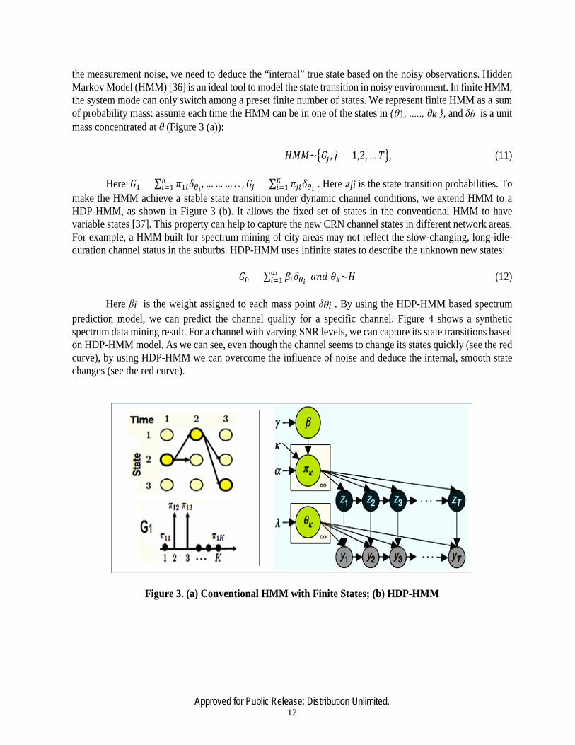
the measurement noise, we need to deduce the “internal” true state based on the noisy observations. Hidden Markov Model (HMM) [36] is an ideal tool to model the state transition in noisy environment. In finite HMM, the system mode can only switch among a preset finite number of states. We represent finite HMM as a sum of probability mass: assume each time the HMM can be in one of the states in θ1, ....., θk , and δθ is a unit mass concentrated at θ (Figure 3 (a)):
𝐻𝐻𝐻𝐻𝐻𝐻~𝐺𝐺𝑗𝑗 , 𝑗𝑗 = 1,2, … 𝑘𝑘, (11) Here 𝐺𝐺1 = ∑ 𝜋𝜋1𝑗𝑗𝛿𝛿𝜃𝜃𝑖𝑖 , … … … . . ,𝐺𝐺𝑗𝑗 = ∑ 𝜋𝜋𝑗𝑗𝑗𝑗𝛿𝛿𝜃𝜃𝑖𝑖
𝐾𝐾𝑗𝑗=1
𝐾𝐾𝑗𝑗=1 . Here πji is the state transition probabilities. To
make the HMM achieve a stable state transition under dynamic channel conditions, we extend HMM to a HDP-HMM, as shown in Figure 3 (b). It allows the fixed set of states in the conventional HMM to have variable states [37]. This property can help to capture the new CRN channel states in different network areas. For example, a HMM built for spectrum mining of city areas may not reflect the slow-changing, long-idle-duration channel status in the suburbs. HDP-HMM uses infinite states to describe the unknown new states:
𝐺𝐺0 = ∑ 𝛽𝛽𝑗𝑗𝛿𝛿𝜃𝜃𝑖𝑖 𝑎𝑎𝑛𝑛𝑎𝑎 𝜃𝜃𝑘𝑘~𝐻𝐻∞𝑗𝑗=1 (12)
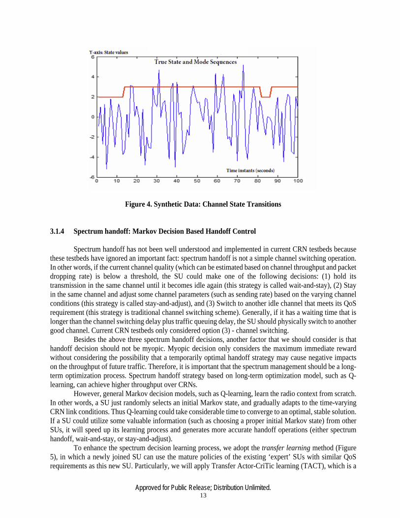
Here βi is the weight assigned to each mass point δθi . By using the HDP-HMM based spectrum prediction model, we can predict the channel quality for a specific channel. Figure 4 shows a synthetic spectrum data mining result. For a channel with varying SNR levels, we can capture its state transitions based on HDP-HMM model. As we can see, even though the channel seems to change its states quickly (see the red curve), by using HDP-HMM we can overcome the influence of noise and deduce the internal, smooth state changes (see the red curve).
Figure 3. (a) Conventional HMM with Finite States; (b) HDP-HMM
Approved for Public Release; Distribution Unlimited. 13
Figure 4. Synthetic Data: Channel State Transitions
3.1.4 Spectrum handoff: Markov Decision Based Handoff Control
Spectrum handoff has not been well understood and implemented in current CRN testbeds because these testbeds have ignored an important fact: spectrum handoff is not a simple channel switching operation. In other words, if the current channel quality (which can be estimated based on channel throughput and packet dropping rate) is below a threshold, the SU could make one of the following decisions: (1) hold its transmission in the same channel until it becomes idle again (this strategy is called wait-and-stay), (2) Stay in the same channel and adjust some channel parameters (such as sending rate) based on the varying channel conditions (this strategy is called stay-and-adjust), and (3) Switch to another idle channel that meets its QoS requirement (this strategy is traditional channel switching scheme). Generally, if it has a waiting time that is longer than the channel switching delay plus traffic queuing delay, the SU should physically switch to another good channel. Current CRN testbeds only considered option (3) - channel switching.
Besides the above three spectrum handoff decisions, another factor that we should consider is that handoff decision should not be myopic. Myopic decision only considers the maximum immediate reward without considering the possibility that a temporarily optimal handoff strategy may cause negative impacts on the throughput of future traffic. Therefore, it is important that the spectrum management should be a long-term optimization process. Spectrum handoff strategy based on long-term optimization model, such as Q-learning, can achieve higher throughput over CRNs.
However, general Markov decision models, such as Q-learning, learn the radio context from scratch. In other words, a SU just randomly selects an initial Markov state, and gradually adapts to the time-varying CRN link conditions. Thus Q-learning could take considerable time to converge to an optimal, stable solution. If a SU could utilize some valuable information (such as choosing a proper initial Markov state) from other SUs, it will speed up its learning process and generates more accurate handoff operations (either spectrum handoff, wait-and-stay, or stay-and-adjust).
To enhance the spectrum decision learning process, we adopt the transfer learning method (Figure 5), in which a newly joined SU can use the mature policies of the existing ‘expert’ SUs with similar QoS requirements as this new SU. Particularly, we will apply Transfer Actor-CriTic learning (TACT), which is a
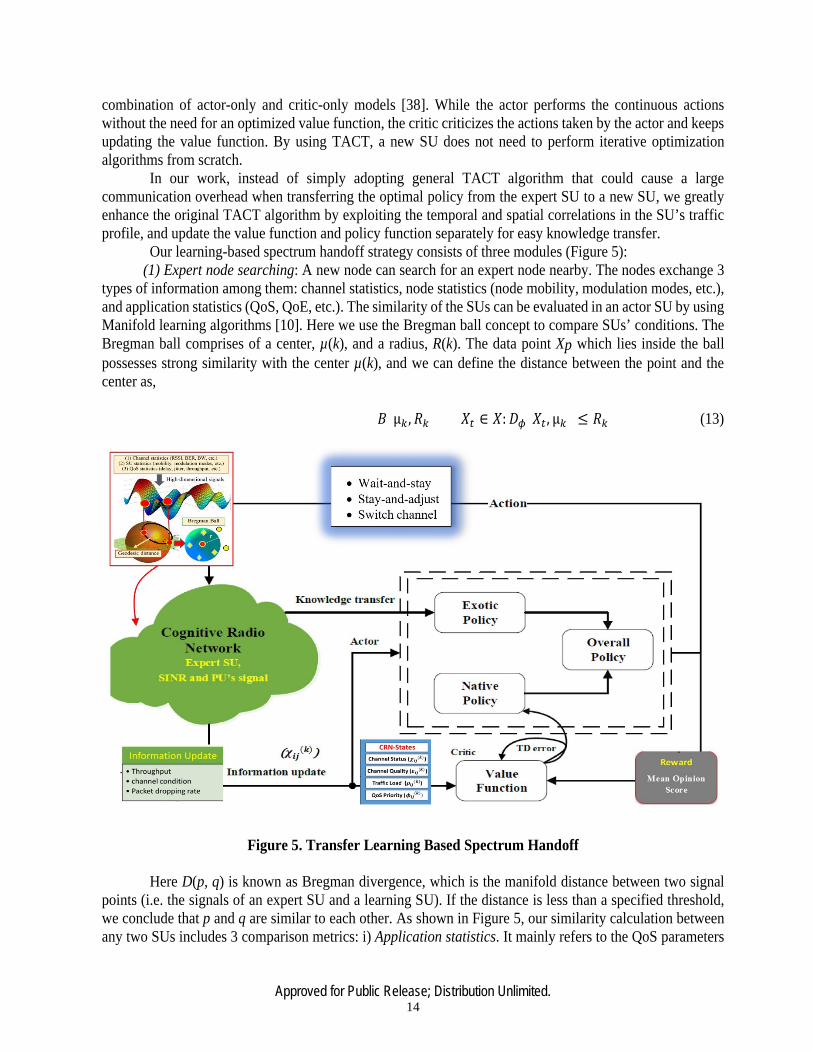
Approved for Public Release; Distribution Unlimited. 14
combination of actor-only and critic-only models [38]. While the actor performs the continuous actions without the need for an optimized value function, the critic criticizes the actions taken by the actor and keeps updating the value function. By using TACT, a new SU does not need to perform iterative optimization algorithms from scratch. In our work, instead of simply adopting general TACT algorithm that could cause a large communication overhead when transferring the optimal policy from the expert SU to a new SU, we greatly enhance the original TACT algorithm by exploiting the temporal and spatial correlations in the SU’s traffic profile, and update the value function and policy function separately for easy knowledge transfer. Our learning-based spectrum handoff strategy consists of three modules (Figure 5): (1) Expert node searching: A new node can search for an expert node nearby. The nodes exchange 3 types of information among them: channel statistics, node statistics (node mobility, modulation modes, etc.), and application statistics (QoS, QoE, etc.). The similarity of the SUs can be evaluated in an actor SU by using Manifold learning algorithms [10]. Here we use the Bregman ball concept to compare SUs’ conditions. The Bregman ball comprises of a center, µ(k), and a radius, R(k). The data point Xp which lies inside the ball possesses strong similarity with the center µ(k), and we can define the distance between the point and the center as,
𝐵𝐵(µ𝑘𝑘 ,𝑅𝑅𝑘𝑘) = 𝑋𝑋𝑡𝑡 ∈ 𝑋𝑋:𝐷𝐷𝜙𝜙(𝑋𝑋𝑡𝑡 , µ𝑘𝑘) ≤ 𝑅𝑅𝑘𝑘 (13)
Figure 5. Transfer Learning Based Spectrum Handoff Here D(p, q) is known as Bregman divergence, which is the manifold distance between two signal points (i.e. the signals of an expert SU and a learning SU). If the distance is less than a specified threshold, we conclude that p and q are similar to each other. As shown in Figure 5, our similarity calculation between any two SUs includes 3 comparison metrics: i) Application statistics. It mainly refers to the QoS parameters
Approved for Public Release; Distribution Unlimited. 15
such as delay, data rates, etc. ii) Node statistics: It includes node modulation modes, location, mobility pattern, etc. iii) Channel statistics: This includes channel parameters such as bandwidth, SNR, etc.
(2) CRN state update: For a given state, the actor selects and executes an action in a stochastic manner. This causes the system to transform from one state to another one with a reward as the feedback to the actor. Then the critic evaluates the action taken by the actor in terms of time difference (TD) error, and updates the value function. After receiving the feedback from the critic, the actor updates the policy. The algorithm repeats itself until it converges. Once the SU chooses an action in channel k, the system changes the state from s to s′ with a transition probability as,
𝑃𝑃(𝑠𝑠′ 𝑠𝑠, 𝑎𝑎) = 1, 𝑠𝑠′ ∈ 𝑆𝑆0, 𝑜𝑜𝑡𝑡ℎ𝑒𝑒𝑟𝑟𝑒𝑒𝑖𝑖𝑠𝑠𝑒𝑒 (14)
Meanwhile, the total reward for the taken action would be Rs.a (here we use the MOS value as the reward). The TD error can be calculated from the difference between (1) the state-value function, V (s), estimated in the previous state, and (2) Rs,a + V (sf) at the critic, as follows:
𝛿𝛿(𝑠𝑠, 𝑎𝑎) = 𝑅𝑅𝑠𝑠,𝑎𝑎 + 𝛾𝛾 𝑃𝑃(𝑠𝑠′|𝑠𝑠, 𝑎𝑎)𝑉𝑉(𝑠𝑠′) − 𝑉𝑉(𝑠𝑠)𝑠𝑠′∈𝑆𝑆
= 𝑅𝑅𝑠𝑠,𝑎𝑎 + 𝛾𝛾𝑉𝑉(𝑠𝑠′) − 𝑉𝑉(𝑠𝑠)
Subsequently, the TD error is sent back to the actor. By using TD error the actor updates its state-value function as
𝑉𝑉(𝑠𝑠′) = 𝑉𝑉(𝑠𝑠) + 𝛼𝛼𝑣𝑣1(𝑠𝑠,𝑚𝑚)𝛿𝛿(𝑠𝑠, 𝑎𝑎) (16) Where ν1(s, m) indicates the occurrence time of state s in m stages. α(.) is a positive step-size
parameter that affects the convergence rate. V (s′) is kept the same as V (s) in case of s = s′.
(3) Policy update: The critic can employ the TD error to criticize the selected action by the actor, and the policy can be updated as [28],
𝑝𝑝(𝑠𝑠, 𝑎𝑎) = 𝑝𝑝(𝑠𝑠, 𝑎𝑎) − 𝛽𝛽𝑣𝑣2(𝑠𝑠, 𝑎𝑎,𝑚𝑚)𝛿𝛿(𝑠𝑠, 𝑎𝑎) (17) Here ν2(s, a, m) denotes the occurrence time of action a at state s in m stages. β(.) denotes the step
size defined by (𝑚𝑚 ∗ 𝑙𝑙𝑜𝑜𝑙𝑙𝑚𝑚)−1[12]. It ensures that an action under a specific state can be selected with a higher probability if we reach the highest minimum reward, i.e. δ(s, a) < 0.
If each action is executed for enough times in each state and the learning algorithm follows a greedy exploration, the value function V (s) and the policy function π(s, a) will ultimately converge to V ∗(s) and π∗ with a probability of 1, respectively.
Formulation of TACT: Initially, the strategy π(s, a) in a learning task is determined by the policy. Let p(s, a) denote the likelihood of taking action a in state s. When the process eventually converges, the likelihood of choosing a particular action a in a particular state s is relatively larger than that of other actions. In other words, if the spectrum handoff is performed based on a learned strategy in SUi, the reward will be the minimum in the long term. Consequently, the knowledge of this policy p(s, a) can be transferred to another SUi which is in the same PU’s coverage and has the same traffic QoS requirement. However, in spite of the similarities between the two SUs, there may still exist some differences. This may make an actor SU take more aggressive actions. To avoid these problems, the transferred policy should have a decreasing impact on the choice of certain actions, especially after the SU has taken its action and cherished its own learning experience. This is the basic idea of TACT-based knowledge transfer with self-learning.
(15)
Approved for Public Release; Distribution Unlimited. 16
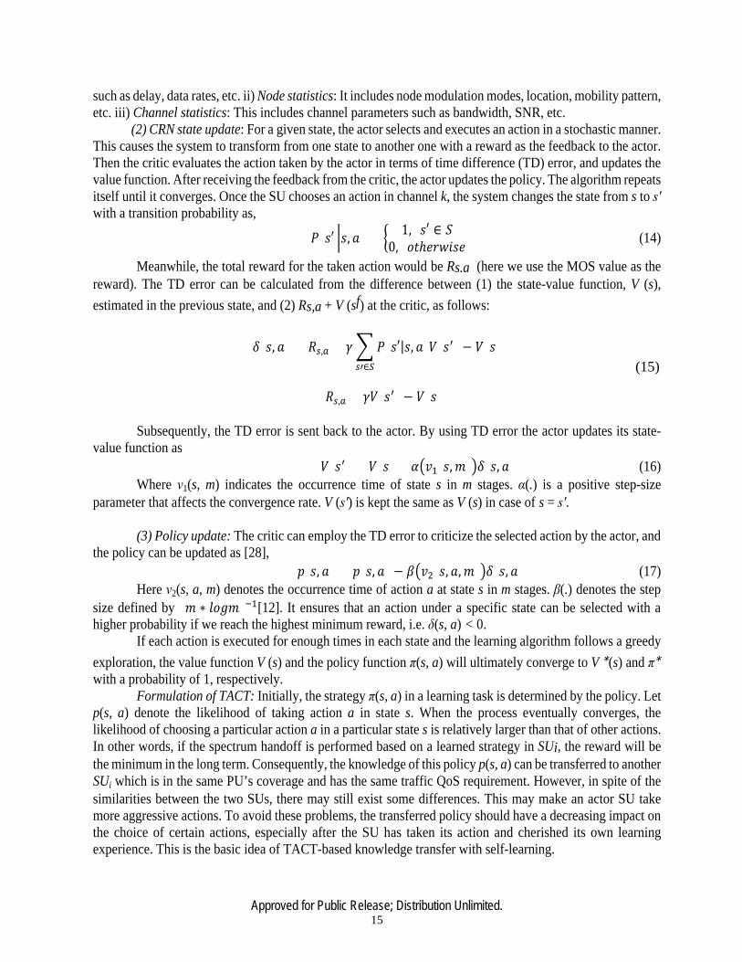
3.1.5 Rateless Codes for Throughput Improvement In our CRN testbed, we have used rateless codes [39] to improve its throughput by avoiding the adjustment of sending rates in highly dynamic channel conditions. Fading and shadowing in wireless channels can cause packet loss and the deterioration of video quality. When a packet loss occurs, the feedback from the receiver can be used for the request of the retransmission for the lost packet. The retransmission- based mechanism is bandwidth-costly. Recently, rateless codes have attracted many attentions. They actually provide a type of Application layer forward error correction (FEC). They can theoretically produce infinite number of encoded symbols from the source symbols, such that the percentage of symbols needed for successful decoding in the receiver can be very small. This makes them especially suitable to noisy wireless communication environments. Raptor codes, which are a class of powerful rateless codes, can completely recover the source data with little overhead and linear encoding/decoding time [40]. The Raptor codes consist of a precode as the outer code and a weakened LT code as the inner code. They can be parameterized by (K, C, Ω(x)), where K is the number of source symbols, C is a precode with blocklength L and dimension K, and Ω(x) is a degree distribution of LT codes. Each encoded symbol is associated with an ID. The precode and weakened LT code can ensure a high decoding probability with a small coding overhead. In our testbed, we use the systematic Raptor codes. If there are K source symbols S[i] in one block, i = 0, ..., K − 1, the first K encoded symbols are constructed such that E[0] = S[0], E[1] = S[1], ..., E[K − 1] = S[K − 1]. The systematic Raptor codes can therefore correctly decode some source symbols even if the number of received encoded symbols (Nr ) is less than the number of source symbols (K). The applications in GNU Radio are primarily written in Python, while some performance-critical components are implemented in C++. The implementation of Raptor codes includes Gaussian Elimination and Belief Propagation. We have implemented Raptor codes in C++. And we have used the SWIG software to transfer some C++ APIs to Python APIs that are called by GNU Radio applications. Our implementation framework of Raptor codes for video transmission over the CRN is shown in Figure 6. As we can see, after the Raptor codes are applied to the original packets in the sender side, they form UDP packets. In the receiver side, after Raptor decoder is applied to the received UDP packets, we use FFplay tool to display the video.
Figure 6. Software Framework: Raptor codes for Video Transmission Over CRN

Approved for Public Release; Distribution Unlimited. 17
3.2 Intelligent Spectrum Management Based on Transfer Actor-Critic Learning (TACT)
In Section 2.1 we mentioned about the TACT-based spectrum handoff scheme. In this section, we describe the details of TACT algorithm and its application to CRN spectrum mobility management. TACT is a special Docitive learning scheme. It emphasizes the node-to-node knowledge transfer process. An optimal spectrum mobility strategy needs to consider its long-term impact on the network performance, such as flow throughput and packet dropping rate, instead of adopting a myopic scheme that optimizes only the short-term throughput. We thus propose to use a promising machine learning scheme, called Transfer Actor-Critic Learning (TACT), for the spectrum mobility strategies. Such a TACT-based scheme shortens a user’s spectrum handoff delay, due to the use of a comprehensive reward function that considers the channel utilization factor (CUF), packet error rate (PER), packet dropping rate (PDR), and flow throughput. Here, the CUF is estimated by a spectrum quality modeling scheme, which considers spectrum sensing accuracy and channel holding time. The PDR is calculated from NPRP M/G/1 queueing model, and the flow throughput is estimated from a link-adaptive transmission scheme, which utilizes the rateless codes. To determine the link throughput, we use a statistical parameter of symbol transmissions called decoding-CDF (cumulative distribution function), which speeds up the link adaptation process when the SU is encountering high PER due to time-varying channel conditions. It also assists with selection of the optimal channel during spectrum handoff. Our simulation results show that the TACT algorithm along with the decoding-CDF model achieves optimal reward value in terms of Mean Opinion Score (MOS), compared to the myopic spectrum decision scheme.
3.2.1 Related Work. In this section, we review the literature directly related to our work, which includes 3 aspects: (1) Learning-based wireless adaptation: The strategy of learning from expert SUs has been used in
our previous work called apprenticeship-learning-based spectrum handoff [10]. Other related work in this direction includes the concept of Docitive learning (DL) [11], [42], reinforcement learning (RL) based CRN throughput improvement [43], RL-based cooperative spectrum sensing [44], and Q-learning based channel allocation [45], [46], etc. DL is successfully used for interference management in Femtocell applications [11]. However, DL does not consider the concrete channel selection parameters. It also does not have clear definitions of expert hunting process and node-to-node similarity calculation functions. A node that sends non-real-time traffic should not become the expert for a node that aims to transmit real-time video. The authors in [8] introduced the channel selection scheme implemented on GNU radio. But they did not consider the CHT and PDR while selecting a channel. The same drawback exists in [45] and [46]. We are also not aware of any related work on TACT-based CRN spectrum handoff designs. The TACT is superior to RL since it can use both node-to-node teaching and self-learning to adapt to the complex CRN spectrum conditions. In addition, we improve the original TACT model by allowing the expert policy to be learned from the Q-values of the RL process.
(2) Channel Selection Metric: The concept of channel selection metric was initially proposed in [10], [47]. A SU selects an idle channel based on channel conditions and queuing delay. In [48], it considers the QoS-based channel selection. But the channel idle duration and channel sensing accuracy have not been taken into consideration. The channel idle duration indicates the period over which a SU can occupy the channel without the interruptions from a PU. The authors in [49] proposed OFDM-based MAC protocol for spectrum sensing and sharing which reduces the sharing overhead extensively. But they did not discuss about the channel types that should be selected by the SU for data transmissions. Our spectrum evaluation scheme considers the comprehensive channel dynamics with respect to the interference, fading loss, and other channel

Approved for Public Release; Distribution Unlimited. 18
i
ij
variations. The channel selection scheme with the consideration of long idle duration and high spectrum detection accuracy, will increase the spectrum utilization efficiency and spectrum handoff accuracy. (3) Decoding-CDF based Spectrum Adaptation: Rateless codes have been used in wireless communications due to its property of recovering the original data with low error rate. The popular rateless codes include Spinal codes [40], [50], Raptor codes [51], Strider codes [52]–[54], etc. Rateless codes for CRNs have been proposed in [38], [42]. The authors of [42] proposed a feedback technique for rateless codes using multi-User MIMO to improve the QoS for wireless services. The authors in [8] used state-of-the-art decoding-CDF with the Spinal codes. In our research we use decoding-CDF along with our own rateless code model - Prioritized Raptor codes (PRC) [9], to perform spectrum adaptation. 3.2.2 TACT-based Spectrum Mobility Management. In this section, we explain our iSM strategy with the following two features: (1) The spectrum decision is made through a throughput optimization model. (2) The channel is selected by considering comprehensive CSM which considers both time variations and spatial variations of the channels. To achieve an intelligent handoff, we first introduce general Q-learning based iSM scheme (as the comparison basis), which simply chooses actions based on SU states. Then we extend it to a TACT-based SU-to-SU teaching model with an expert node’s assistance during the handoff decision. We will explain how we seek an expert SU that knows how to make correct handoff decisions under different node states, and how the expert SU can speed up the new SU’s learning process by transferring proper iSM parameters to it. 3.2.2.1 Channel Selection Metric. In order to select a good channel during spectrum handoff, the SU should understand the temporal and spatial characteristics of the channel. The time-varying characteristics comprises of CHT and PDR. Whereas spatial characteristics comprises of achievable throughput and PER. 3.2.2.2 Channel Utilization factor (CUF): Here we directly provide its result for discussion convenience (Later on we will describe how to calculate CUF):
𝐶𝐶𝐶𝐶𝐶𝐶 = 𝐻𝐻𝐴𝐴∙𝑡𝑡
(𝑁𝑁−𝜏𝜏) 1 − 𝑒𝑒−(𝑇𝑇−𝜏𝜏)𝑡𝑡 (18)
According to IEEE 802.22 recommendations, the probability of correct detection, Pd = [0.9, 0.99], and the probability of false alarm, Pf = [0.01, 0.1]. Therefore, the probability of spectrum sensing accuracy is Pd(1 − Pf ) = [0.81, 0.99].
3.2.2.3 PU/SU NPRP-M/G/1 Queuing Model. We define a non-preemptive M/G/1 model where the SU with the lowest priority accesses the channel without the interruptions from higher priority SUs. Denote j=1 as the highest priority and j=N as the lowest one. But any SU transmissions can be interrupted by a PU. Once the channel becomes idle, the SU with higher priority will be served. In our previous work [6], we have deduced the packet drop rate (PDR) in a link lij for a channel k with packet arrival rate, λ, and mean service rate, µ, as:
𝑃𝑃𝐷𝐷𝑅𝑅𝑗𝑗𝑗𝑗(𝑘𝑘) = 𝑝𝑝𝑗𝑗𝑗𝑗
(𝑘𝑘). exp (−𝑝𝑝𝑖𝑖𝑖𝑖
(𝑘𝑘)×𝑑𝑑𝑖𝑖−𝐷𝐷𝐷𝐷𝐷𝐷𝑎𝑎𝐷𝐷𝑖𝑖𝑖𝑖
𝐸𝐸𝐷𝐷𝑖𝑖(𝑘𝑘)𝑗𝑗
) (19)
For ith interruption, the handoff delay is E[D(k)j], and the probability that the handoff delay is more than packet active period (dj − Delayji), is (𝑑𝑑𝑗𝑗 − 𝐷𝐷𝐷𝐷𝐷𝐷𝑎𝑎𝐷𝐷𝑗𝑗𝑗𝑗)
𝐸𝐸[𝐷𝐷𝑗𝑗(𝑘𝑘)𝑗𝑗] . Therefore, the term (dj − Delayji) determines the
left-over active period of the packet associated with the SUj . If such an active period is more than the average waiting delay, the PDR will be low. Besides, 𝑝𝑝𝑗𝑗𝑗𝑗
(𝑘𝑘)is the normalized load of the channel k between node i and

Approved for Public Release; Distribution Unlimited. 19
j
j. It is defined as follows,𝑝𝑝𝑗𝑗𝑗𝑗
(𝑘𝑘) = 𝜆𝜆𝑖𝑖µ𝑘𝑘≤ 1 (20)
When the average delay exceeds the delay limit (dj −Delayji), the packet will be dropped. Here dj rrepresents the maximum delay that can be tolerated by type-j SU, and Delayji denotes the actual delay experienced by the type − j SU due to network congestion. E[D(k)] is the average delay (an expectation value)experienced by each SU in channel k.
3.2.2.4 CDF-Enhanced Throughput. Using the decoding-CDF [8] we can estimate the achievable throughput (TH) in a Rayleigh fading channel as follows (its deduction process will be explained later),
𝑘𝑘𝐻𝐻𝑗𝑗𝑗𝑗(𝑘𝑘) = 2×𝑖𝑖𝑠𝑠×(𝑁𝑁𝑆𝑆)
𝑡𝑡 𝑠𝑠𝑦𝑦𝑚𝑚𝑠𝑠𝑜𝑜𝑙𝑙𝑠𝑠/𝑠𝑠/𝐻𝐻𝐻𝐻 (21)
The normalized throughput is:
(𝑘𝑘𝐻𝐻𝑗𝑗𝑗𝑗(𝑘𝑘))𝑛𝑛𝑛𝑛𝑛𝑛𝑚𝑚 =
𝑁𝑁𝑇𝑇𝑖𝑖𝑖𝑖(𝑘𝑘)
(𝑁𝑁𝑇𝑇𝑖𝑖𝑖𝑖(𝑘𝑘))𝑖𝑖𝑖𝑖𝑖𝑖𝑖𝑖𝑖𝑖
(22)
Where fs, t, N S are the sampling frequency, transmission time, and the number of symbols per packet, respectively. They will be described later. Here, (TH(k))ideal is the ideal throughput calculated via Shannoncapacity theorem.
We perform the normalization of each throughput by considering the ideal scenario, i.e. Shannon capacity. And our final goal is to find a suitable spectrum handoff strategy by using such a normalized throughput. Using different channel models does not affect our handoff strategy since our learning algorithm can optimize the spectrum decision process by considering the highest normalized throughput among the available channels.
Now we can integrate the above 3 models together into the CSM, through a weighted channel selection metric for SUi,
𝐶𝐶𝑗𝑗𝑗𝑗(𝑘𝑘) = 𝑒𝑒1 ∗ 𝐶𝐶𝐶𝐶𝐶𝐶 + 𝑒𝑒2 ∗ 1 − 𝑃𝑃𝐷𝐷𝑅𝑅𝑗𝑗𝑗𝑗
(𝑘𝑘) + 𝑒𝑒2 ∗ (𝑘𝑘𝐻𝐻𝑗𝑗𝑗𝑗(𝑘𝑘))𝑛𝑛𝑛𝑛𝑛𝑛𝑚𝑚 (23)
Where w1, w2 and w3 are weighted coefficients representing the relative importance levels of the channel quality, PDR, and throughput, respectively. Their setup depends on application QoS requirements. For real-time applications, the throughput is more important than PDR. For FTP applications, PDR is the most important factor. For video applications, CHT (part of CUF model) is more important. Here w1 + w2 + w3 = 1.
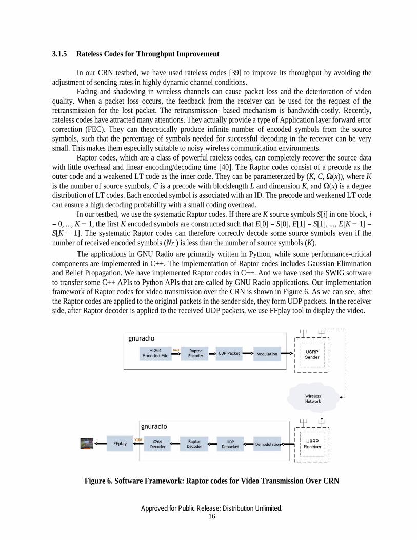
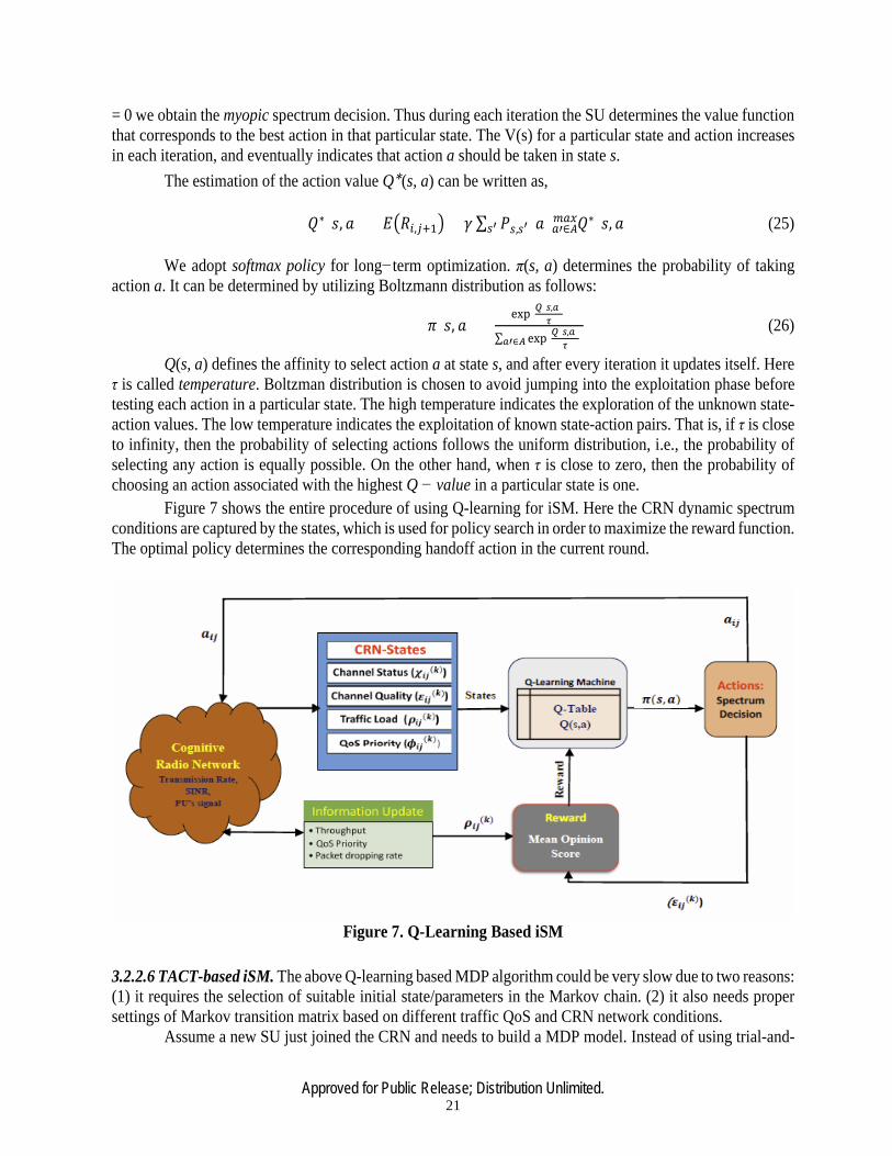
3.2.2.5 Q-Learning based iSM: To serve as the comparison basis for our TACT-based learning scheme, we will first describe the use of a popular self- learning method, Q-learning, for the determination of suitable handoff actions in each SU state. Q-learning is a special Markov Decision Process (MDP), which can be stated as a tuple (S, A, T, R) [43], where S depicts the set of system states, A is the set of system actions in each state. T represents the transition probability, where T = P (s, a, st), here P (.) the probability of transition from state s to sf when action a is being taken, and 𝑅𝑅: 𝑆𝑆 × 𝐴𝐴 → 𝑅𝑅 is the reward or cost function, which depicts the reward for taking an action a ∈ A in state s ∈ S. In MDP, we intend to find the optimal policy π∗(s) ∈ A, i.e., a series of actions a1, a2, a3, ... for state s, in order to maximize the total discount reward function.
States: For SUi, the network state before (𝑗𝑗 + 1)𝑡𝑡ℎ channel assignment is depicted as sij

Approved for Public Release; Distribution Unlimited. 20
ij ij
=𝑥𝑥𝑗𝑗𝑗𝑗(𝑘𝑘), 𝛽𝛽𝑗𝑗𝑗𝑗
(𝑘𝑘), 𝑝𝑝𝑗𝑗𝑗𝑗(𝑘𝑘), 𝜉𝜉𝑗𝑗𝑗𝑗
(𝑘𝑘),𝜙𝜙𝑗𝑗𝑗𝑗(𝑘𝑘), where k is the channel being used. χ(k) depicts the status of the channel (idle or
busy). ξ(k) states the quality of the channel k (i.e., the above discussed comprehensive channel metric, CSM). ρ(k)indicates the traffic load of the channel k. Lastly, φ(k) represents the QoS priority level of SUi. Actions: Three actions are considered in the iSM scheme: (1) stay-and-await: stay in the same channel and hold the traffic until the channel’s CSM is above a preset threshold; (2) stay-and-adjust (transmit more or less symbols) until the required MOS value is met after using decoding-CDF, and (3) spectrum handoff : jump to a new channel with the best CSM; We denote aij = β(k) ∈ A as the candidate actions for SUi on state sij after the assignment of (j + 1)th channel. β(k) represents the probability of choosing action aij. The Q-learning algorithm aims to find an optimal action which minimizes the expected cost at the current policy π∗(si,j , ai,j ) in the process of (j + 1)th channel assignment to SUi. It is based on the value function that determines how good it is for a given agent to perform a certain action under a given state. The term good here is defined in terms of value function V π (s), which is known as state-value function for a policy π. In a similar fashion we define the value of taking action a (i.e., how good it is to take action a) in state s given the policy π. It is also called as action value function Qπ (s, a). It tells which action has low cost in the long term. Bellman optimality equation [55] gives the high, discounted long-term rewards. For the sake of simplicity, we consider si,j as s, action ai,j as a , and state si,j+1 as sf. Rewards: The reward R is defined as the immediate cost incurred for the multimedia transmissions. The reward is a measure of multimedia Quality of Experience (QoE), defined as Mean Opinion Score (MOS) [2]. When the channel status in idle, ‘transmission’ is an ideal action to take, which would incur a MOS close to 5. On the other hand, when PDR (belonging to the state of Traffic load) or PER (belonging to the state of Channel quality) are high, it would incur low MOS that reflects the poor performance in the channel. If the value of MOS is below the desired threshold value, M OSth, then SU takes the spectrum decision according to the following rule, Rule-1: Spectrum Decision Rule if ts ≤ tw , P ER ≥ P ERth and P DR ≥ P DRth then determine the best channel using CSM and perform spectrum handoff. This is real spectrum handoff. else if ts > tw and P ER ≥ P ERth, then stay-and-transmit the required number of symbols using decoding-CDF. This is stay-and-adjust. else if ts > tw and P DR ≥ P DRth, then stay-and-wait until the channel becomes idle or good. This is called stay-and-wait. end Where ts, tw, PDRth and PERth are the channel switching time, channel waiting time, PDR threshold, and PER threshold respectively. Both switching delay ts and waiting delay tw , are calculated from our defined NPRP-M/G/1 queueing model. Using MOS in the reward function helps Q-learning algorithm to accurately model the video QoE performance during the spectrum handoff. During the process we update the parameter V (s), i.e. the value function. Value function determines how good it is for a given agent to perform a certain action under a given state. The value function can be defined as V (s):
𝑉𝑉𝜋𝜋(𝑠𝑠) = 𝐸𝐸𝑅𝑅𝑗𝑗,𝑗𝑗+1 + 𝛾𝛾𝑎𝑎∈𝐴𝐴𝑚𝑚𝑎𝑎𝑥𝑥 ∑ 𝑃𝑃𝑠𝑠,𝑠𝑠′(𝑎𝑎)𝑠𝑠′ 𝑉𝑉𝜋𝜋(𝑠𝑠′) (24)
Where 0 ≤ 𝛾𝛾 ≤ 1 is the discount factor which reduces the impact of the preceding actions. Setting 𝛾𝛾 γ
Approved for Public Release; Distribution Unlimited. 21
= 0 we obtain the myopic spectrum decision. Thus during each iteration the SU determines the value function that corresponds to the best action in that particular state. The V(s) for a particular state and action increases in each iteration, and eventually indicates that action a should be taken in state s.
The estimation of the action value Q∗(s, a) can be written as,
𝑄𝑄∗(𝑠𝑠, 𝑎𝑎) = 𝐸𝐸𝑅𝑅𝑗𝑗,𝑗𝑗+1 + 𝛾𝛾 ∑ 𝑃𝑃𝑠𝑠,𝑠𝑠′(𝑎𝑎) 𝑄𝑄∗(𝑠𝑠, 𝑎𝑎)𝑎𝑎′∈𝐴𝐴𝑚𝑚𝑎𝑎𝑥𝑥
𝑠𝑠′ (25)
We adopt softmax policy for long−term optimization. π(s, a) determines the probability of taking action a. It can be determined by utilizing Boltzmann distribution as follows:
𝜋𝜋(𝑠𝑠, 𝑎𝑎) =exp (𝑄𝑄(𝑠𝑠,𝑖𝑖)
𝜏𝜏 )
∑ exp (𝑄𝑄(𝑠𝑠,𝑖𝑖)𝜏𝜏 )𝑖𝑖′∈𝐴𝐴
(26)
Q(s, a) defines the affinity to select action a at state s, and after every iteration it updates itself. Here τ is called temperature. Boltzman distribution is chosen to avoid jumping into the exploitation phase before testing each action in a particular state. The high temperature indicates the exploration of the unknown state-action values. The low temperature indicates the exploitation of known state-action pairs. That is, if τ is close to infinity, then the probability of selecting actions follows the uniform distribution, i.e., the probability of selecting any action is equally possible. On the other hand, when τ is close to zero, then the probability of choosing an action associated with the highest Q − value in a particular state is one.
Figure 7 shows the entire procedure of using Q-learning for iSM. Here the CRN dynamic spectrum conditions are captured by the states, which is used for policy search in order to maximize the reward function. The optimal policy determines the corresponding handoff action in the current round.
Figure 7. Q-Learning Based iSM
3.2.2.6 TACT-based iSM. The above Q-learning based MDP algorithm could be very slow due to two reasons: (1) it requires the selection of suitable initial state/parameters in the Markov chain. (2) it also needs proper settings of Markov transition matrix based on different traffic QoS and CRN network conditions.
Assume a new SU just joined the CRN and needs to build a MDP model. Instead of using trial-and-

Approved for Public Release; Distribution Unlimited. 22
error style to seek proper MDP settings, it may find a neighboring SU with similar traffic QoS demands, and asks it to serve as an “expert” (or “teacher”) that will transfer all optimal policies to itself. Such teaching-based strategy can largely shorten the learning convergence time. Specifically, we propose to use TACT model for the knowledge transfer between SUs. TACT [12] composes of three components: actor, critic and environment. For a given state, the actor selects and executes an action in a stochastic manner. This causes the system to transform from one state to another one, with a reward as the feedback to the actor. Then the critic evaluates the action taken by the actor in terms of time difference (TD) error, and updates the value function. After receiving the feedback from the critic, the actor updates the policy. The algorithm repeats until it converges. To apply TACT to CRN spectrum decision, we need to solve two critical issues: Who should be the expert SU? Here we consider distributed network where there is no central coordinator which controls other SUs in the network. When the new SU joins the network it will do the localized search and broadcasts EXPERT-SEEK information. As a matter of fact, the nodes nearby may be located in the area covered by the same PU(s), and thus have similar spectrum availability. The SU should select a critic SU based on the relevancy with its application, the level of expertness, and the influence of an action on the link conditions. To find an expert SU, the SUs should share 3 types of information among themselves, i.e., channel statistics (such as CUF), node statistics (node mobility, modulation modes, etc.), and application statistics (QoS, QoE, etc.). The similarity of the SUs can be evaluated in an actor SU by using several similarity estimation techniques such as Manifold learning [10]. Manifold learning uses the Bregman Ball concept to compare complex objects. The Bregman ball comprises of a center, µ(k) and a radius, R(k). The data point Xp which lies inside the ball possesses strong similarity with the center µ(k), and we define their distance as,
𝐵𝐵(µ𝑘𝑘 ,𝑅𝑅𝑘𝑘) = 𝑋𝑋𝑡𝑡 ∈ 𝑋𝑋:𝐷𝐷𝜙𝜙(𝑋𝑋𝑡𝑡 , µ𝑘𝑘) ≤ 𝑅𝑅𝑘𝑘 (27) Here D(p, q) is known as Bregman Divergence, which is the manifold distance between two signal points (an expert SU and a learning SU). If the distance is less than a specified threshold, we conclude that p and q are similar to each other. All distances are visualized in Gephi (a network analysis and visualization software) [6], as shown in Figure 8.
Figure 8. Gephi-Simulated Expert SU Searching As we can see, our similarity calculation between any two SUs includes 3 comparison metrics: (1) application statistics. It mainly refers to the QoS parameters such as delay, data rates, etc. (2) node statistics:

Approved for Public Release; Distribution Unlimited. 23
it includes node modulation modes, location, mobility pattern, etc. (3) channel statistics: this includes channel parameters such as bandwidth, SNR, etc. The SU with the highest similarity value with the learning SU is chosen as the expert SU. In Figure 8, SU3 is selected as the expert SU (i.e., the critic) since it has higher similarity to the learning SU, compared to the rest of the SUs. (SU1 is the learner here).
Therefore, our expert SU searching scheme considers both QoS requirement and radio conditions (such as node mobility/location, traffic profile, channel statistics, etc.). Here, exchanging expert policy increases the communication intelligence of the whole network. Thus the expert SU is willing to share the information with a new SU.
How to transfer the node knowledge via TACT model? The actor-critic learning separately updates the value function and policy function. It paves an easier way to transfer the policy knowledge than other critic-only schemes such as Q-learning and c-greedy policy. We implement TACT-based iSM as follows:
Action selection: When a new SU joins the network, the initial state is sij in channel k. In order to optimize the performance, the SU chooses actions to balance two explicit functions: a) searching for the new channel if the current channel condition degrades (exploration), and b) finding an optimal policy by sticking to the current channel (exploitation). This also enables the SU not only to explore a new channel but also to find the optimal policy based on its past experience.
Reward: The Mean Opinion Score (MOS) is used as the reward that corresponds to a action a ∈ A taken in state s∈ S.
State-value function update: Once the SU chooses an action in channel k , the system changes the state from s to s’ with a transition probability,
𝑃𝑃(𝑠𝑠′ 𝑠𝑠, 𝑎𝑎) = 1, 𝑠𝑠′ ∈ 𝑆𝑆0, 𝑜𝑜𝑡𝑡ℎ𝑒𝑒𝑟𝑟𝑒𝑒𝑖𝑖𝑠𝑠𝑒𝑒 (28)
Meanwhile, the total reward for the taken action would be Rs.a = MOS. The TD error can be calculated from the difference between (1) the state-value function V (s), estimated in the previous state, and (2) Rs,a + V (sf) at the critic [5],
𝛿𝛿(𝑠𝑠, 𝑎𝑎) = 𝑅𝑅𝑠𝑠,𝑎𝑎 + 𝛾𝛾 𝑃𝑃(𝑠𝑠′|𝑠𝑠, 𝑎𝑎)𝑉𝑉(𝑠𝑠′) − 𝑉𝑉(𝑠𝑠)𝑠𝑠′∈𝑆𝑆
= 𝑅𝑅𝑠𝑠,𝑎𝑎 + 𝛾𝛾𝑉𝑉(𝑠𝑠′) − 𝑉𝑉(𝑠𝑠) Subsequently, the TD error is sent back to the actor. By using TD error the actor updates its state-
value function as: 𝑉𝑉(𝑠𝑠′) = 𝑉𝑉(𝑠𝑠) + 𝛼𝛼(𝑣𝑣1(𝑠𝑠,𝑚𝑚))𝛿𝛿(𝑠𝑠, 𝑎𝑎) (30)
Where ν1(s, m) indicates the occurrence time of the state s in these m stages. α(.) is a positive step-size parameter that affects the convergence rate. V (sf) is kept the same as V (s) in case of s ;= sf.
Policy update: The critic would employ the TD error to criticize the selected action by the actor, and the policy can be updated as [28],
𝑝𝑝(𝑠𝑠, 𝑎𝑎) = 𝑝𝑝(𝑠𝑠, 𝑎𝑎) − 𝛽𝛽(𝑣𝑣2(𝑠𝑠, 𝑎𝑎,𝑚𝑚))𝛿𝛿(𝑠𝑠, 𝑎𝑎) (31) Here ν2(s, a, m) denotes the occurrence time of action a at state s in these m stages. β(.) denotes the
step size defined by (m ∗ logm)-1 [12]. The above model ensures that one action under a specific state can be selected with a higher probability if we reach the highest minimum reward, i.e., δ(s, a) < 0. If each action is executed for enough times in each state and the learning algorithm follows a greedy exploration, the value function V (s) and the policy function π(s, a) will ultimately converge to V ∗(s) and π∗ with a probability of 1, respectively.
Formulation of TACT: Initially, the strategy π(s, a) in a learning task is determined by the policy. Let
(29)

Approved for Public Release; Distribution Unlimited. 24
p(s, a) denote the likelihood of taking action a in state s. When the process eventually converges, the likelihood of choosing a particular action a in a particular state s is larger than that of other actions. In other words, if the spectrum handoff is performed based on a learned strategy by SUi, the reward will be the minimum in the long term. Consequently, the knowledge of this policy p(s, a) can be transferred to another SUi which is in the same PU’s coverage and has the same traffic QoS requirement. However, in spite of the similarities between the two SUs, there might still exist some differences. This may make an actor SU take more aggressive actions. To avoid these problems, the transferred policy should have a decreasing impact on the choice of certain actions, especially after the SU has taken its action and cherished its own learning experience. This is the important feature of TACT-based decision with knowledge transfer and self-learning. The new policy update follows TACT principle (see Figure 9), in which the overall policy of selecting an action is divided into a native policy, pn and an exotic policy, pe. Assume at stage m, the state is s and the chosen action is a. The overall policy can be updated as [8]:
𝑝𝑝𝑛𝑛(𝑚𝑚+1)(𝑠𝑠, 𝑎𝑎) = [(1 − 𝜔𝜔𝑣𝑣2(𝑠𝑠, 𝑎𝑎,𝑚𝑚)𝑝𝑝𝑛𝑛(𝑚𝑚+1)(𝑠𝑠, 𝑎𝑎) + 𝜔𝜔𝑣𝑣2(𝑠𝑠, 𝑎𝑎,𝑚𝑚)𝑝𝑝𝐷𝐷(𝑚𝑚+1)(𝑠𝑠, 𝑎𝑎)] 𝑝𝑝𝑡𝑡−𝑝𝑝𝑡𝑡
(32) Where [𝑥𝑥] 𝑏𝑏𝑎𝑎, (b > a), indicates the Euclidean distance of interval [a,b], i.e., [𝑥𝑥] 𝑏𝑏𝑎𝑎 = a if x < a; [𝑥𝑥] 𝑏𝑏𝑎𝑎 = b if x < b; and [𝑥𝑥] 𝑏𝑏𝑎𝑎 = x if a ≤ x ≤ b.In this scenario, a = −pt and b = pt. In addition, 𝑝𝑝𝑛𝑛(𝑚𝑚+1)(𝑠𝑠, 𝑎𝑎) = 𝑝𝑝𝑛𝑛(𝑚𝑚)(𝑠𝑠, 𝑎𝑎), ∀a ∈ A but a ;= aij . And pn(s, a)updates itself according to equation (15). During the initial learning process, the exotic policy pe(s, a) influences the overall learning strategy. Therefore, when the SU enters a state s , the presence of pe(s, a) forces it to choose the action, which might be optimal to the expert SU . Subsequently, the policy update strategy can bring a performance jumpstart. We define ω ∈ (0, 1) as the transfer rate, and ω 1→ 0 as the number of iterations goes to ∞. Thus eventually it deceases the effect of exotic policy pe(s, a). This means that a SU will not take the learned experience from the expert SU, and thus is able to avoid the negative guidelines from the expert SU. Algorithm 1 describes our TACT-based iSM scheme.
Figure 9. TACT Based SU-to-SU Teaching.

Approved for Public Release; Distribution Unlimited. 25
Algorithm 1. TACT-Based Spectrum Decision Scheme
3.2.3 Channel Utilization Determination
This section will explain how to determine a component of CSM, i.e. CUF. A good channel can be a candidate that a spectrum handoff operation will switch to, if the existing channel has poor quality. While selecting a channel, a busy channel may be detected as idle. This misinterpretation is called as false alarm. The false alarm largely affects the desired QoS, since the channel selection process may end up with selecting a poor channel. Hence, we consider the false alarm rate of channel sensing as the key parameter to gauge the accuracy of spectrum sensing. We consider spectrum sensing accuracy and CHT as two metrics to evaluate the channel utilization. From [7], we know that a higher detection probability, Pd, comes with a low false alarm probability, Pf . Hence we express the accuracy of the spectrum sensing as
𝐻𝐻𝐴𝐴 = 𝑃𝑃𝑑𝑑1 − 𝑃𝑃𝑖𝑖 (33) In addition, the CHT associated with channel − k is determined by
t = 1𝜆𝜆𝑝𝑝ℎ
(34)
Denote T as the total frame length with τ (the channel sensing time), as shown in Figure 10.

Approved for Public Release; Distribution Unlimited. 26
Obviously, equation (18) represents the average idle duration of the P Uk . We assume that the arrival rate of PU follows Poisson distribution and its pdf f (t) follows an exponential distribution within a duration t, as follows,
Figure 10. Frame Transmission Pattern
𝑓𝑓(𝑡𝑡) = 𝜆𝜆𝑝𝑝ℎ𝑒𝑒−𝜆𝜆𝑝𝑝ℎ𝑡𝑡 (35) Since PU’s arrival time is unpredictable, the PU can come and interfere with the SU’s transmission at any time. Hence, the predictable interruption duration [54] can be determined as,
𝑦𝑦(𝑡𝑡) = 𝑘𝑘 − 𝜏𝜏 − 𝑡𝑡, 0 ≤ 𝑡𝑡 ≤ (𝑘𝑘 − 𝜏𝜏)0, 𝑡𝑡 ≥ (𝑘𝑘 − 𝜏𝜏) (36)
Meantime, the SU transmits the data with an average collision duration as [54]
𝑦𝑦(𝑘𝑘) = 1 − ∫ (𝑘𝑘 − 𝜏𝜏 − 𝑡𝑡)𝑓𝑓(𝑡𝑡)𝑎𝑎(𝑡𝑡) = (𝑘𝑘 − 𝑡𝑡) − 𝑡𝑡(1 − 𝑒𝑒−(𝑇𝑇−𝜏𝜏)𝑡𝑡 )𝑁𝑁−𝜏𝜏
0 (37) Hence, the probability that an SU experiences the interference from an PU within its frame transmission duration is given by
𝑃𝑃𝑝𝑝𝑠𝑠 = 𝐷(𝑁𝑁)(𝑁𝑁−𝜏𝜏)
= 1 − 𝑡𝑡(𝑁𝑁−𝜏𝜏)
(1 − 𝑒𝑒−(𝑇𝑇−𝜏𝜏)𝑡𝑡 ) (38)
The parameter that defines the total channel utilization, i.e. CUF, is determined using CHT and probability of having interference from PU. It can be determined as,
𝐶𝐶𝐶𝐶𝐶𝐶 = 𝐻𝐻𝐴𝐴(𝑁𝑁−𝜏𝜏)𝑁𝑁
1 − 𝑃𝑃𝑝𝑝𝑠𝑠 (39)
Thus the CUF can be re-written as follows,
𝐶𝐶𝐶𝐶𝐶𝐶 = 𝐻𝐻𝐴𝐴∙𝑡𝑡
(𝑁𝑁−𝜏𝜏) 1 − 𝑒𝑒−(𝑇𝑇−𝜏𝜏)𝑡𝑡 (40)
The above CUF can be used to represent the spectrum evaluation result for the selection of an optimal channel. It has been used in the expression of CSM. 3.2.4 Throughput Determination in Decoding-CDF based Rateless Transmissions This section will explain how we can determine another component of CSM, i.e. traffic throughput in rateless transmissions. After we accurately identify a high-CUF channel, the next step is to transmit the SU’s packets in this channel. Due to spatial variation, even a channel with high CUF could have time-varying link quality due to the mobility of the SU. Therefore, link adaptation is a critical operation in CRNs. Without efficient link adaptation, the spectrum handoff can occur frequently.

Approved for Public Release; Distribution Unlimited. 27
Generally, the sender needs to adjust its sending rates based on the channel conditions since a poor link can cause high packet loss rate. As an example, in 802.11 links, the sender measures a link’s signal-to-noise ratio (SNR), and uses it to determine the densest constellation diagram with different modulation modes and varying coding rates. Table 1 shows an example. Here the coding rate is defined as the ratio of the original data bits to the encoded bits.
TABLE 1. An Example of Channel Adaptation
NR Threshold Bitrate Modulation Coding Rates>4dB 8Mbps BPSK 3/4>5dB 12Mbps QPSK 1/2>12dB 24Mbps 16-QAM 3/4>21dB 48Mbps 64-QAM 2/3
However, such a channel adaptation may not be accurate since the link SNR is based on last-time measurement (often through the feedback from the receiver). Moreover, the cases shown in Table V are highly “discrete”, that is, the sender cannot achieve a smooth rate adjustment since only a limited number of adaptation rates are available. Because channel condition variations can occur in very short time scales (even in sub-packet level), it is challenging to adapt to the dynamic link conditions in CRNs.
Rateless codes, also called “regret-free” codes, have been shown effective in multimedia over CRNs [55]. They treat all symbols (i.e. coded packets) equally, i.e. no symbol is discarded. In the sender side, each group of packets is decomposed into some symbols with certain redundancy such that the receiver can easily reconstruct the original packets as long as enough number of symbols are received. The sender does not need to change the modulation and encoding schemes. It simply keeps sending the symbols until an ACK is received, which means that the receiver has obtained enough symbols to reconstruct the original packets. The sender then sends out the next group of symbols. For a well-designed rateless code, the number of sent symbols closely tracks the changes in the channel conditions.
In this section, we will first explain our invented unequal error protection (UEP) based Fountain codes, which is an efficient rateless code for real-time multimedia transmission over CRNs. Then we will describe how we can achieve cognitive link adaptation through the self-learning of historical ACK feedback statistics (such as inter-arrival time gaps between two feedbacks). We will show how an SU can build a decoding-CDF using previously transmitted symbols and how it can be used for channel selection and link adaptation strategies.
In rateless codes, after sending certain number of symbols, the sender pauses the transmission to wait for a feedback (ACK) from the receiver. The decoding-CDF defines the probability of successfully decoding a packet from the received symbols. typically it takes at least a few milli-seconds (ms) to finish a single round of group transmission [8], which includes the following time-consuming operations in both the sender and receiver: (1) the receiver switches its radio circuit from Rx (receiving) to Tx (transmission) modes. (2) The receiver completes the ongoing rateless decoding and determines whether a positive ACK should be sent back; (3) it forms ACK packet; (4) it turns radio back to Tx; (5) the sender switches from Tx to Rx and decodes ACK, and then stops sending more symbols for the acknowledged packet group; (6) it turns back to Tx to send out new symbols for the next group of packets. It has shown in [8] that each pause for ACK wastes 18% of overhead in terms of the total time spent on symbol transmission plus ACK feedback.
Figure 11 clearly shows the benefit of using CDF. Without CDF (Figure 11 left), the sender has to pause after sending the minimum number of symbols for each group (those symbols ensure the complete recovery of the original packets). If the receiver still cannot re-assemble G#1 (Group 1), then no ACK will

Approved for Public Release; Distribution Unlimited. 28
be sent back. The sender has to send extra symbols for G#1 packets. After using CDF (Figure 11 right), since the sender already has the statistical distribution about how many symbols it should send before each pause, it can choose to pause at a proper time after sending the minimum number of G#1 symbols plus some extra ones (just in case the receiver needs more symbols for packet reconstruction). Because the ACK takes some time to get back to the sender side, the sender can just squeeze part of G#2 symbols before its first pause. As we can see from Figure 11 (right), while the ACK for G#1 is on the way, the sender has sent out quite a few symbols for both G#1 and G#2, and then pauses at the right time to wait for ACK of G#1. We determine decoding-CDF by using our invented UEP-based Fountain codes, which assign different priorities to different packets, and give higher priority packets more redundancy of symbols (Figure 12). Such a prioritized rateless code can support higher transmission reliability for more critical data.
Figure 11. Benefits of Using CDF: (Left) No CDF Case; (Right) Using CDF
3.2.5 CDF-Enhanced Fountain Codes The CDF is defined as the probability with which the encoded message can be decoded successfully without errors, after a certain number of symbols have been received by the decoder. Obviously the probability distribution increases monotonically with the number of symbols received. This distribution is sensitive to code parameters, channel conditions, and code block length. Surprisingly, we just need to collect a small amount of records on the relationship between n (number of symbols sent between two consecutive pauses) and τ (ACK feedback delay), in order to obtain the CDF curve [8]. The main features of decoding CDF include: 1) since it pauses at the right times, it thus implicitly captures all the channel uncertainties in CRN. 2) It can maximize the throughput of CRN traffic due to the avoidance of unnecessary pauses. In order to speed up the CDF learning process, Gaussian approximation can be adopted. Gaussian approximation is a reasonable approximation at low SNR, and its maximum likelihood (ML) only requires the mean, µ and variance, σ2. In addition, we introduce the parameter α, which ranges from 0 (means no memory) to 1 (unlimited memory), to represent the importance of historic symbols in the calculation. This process has two advantages: first, the start-up transition dies out quickly, and second, the ML estimator is well behaved for α = 1. Algorithm-2 defines the Gaussian CDF learning process.

Approved for Public Release; Distribution Unlimited. 29
Figure 12. Prioritized Fountain Codes
Algorithm 2. Decoding CDF Estimation
By using Algorithm-2 the decoding-CDF can be estimated using the standard Gaussian equation,
𝐶𝐶(𝑥𝑥) = ∫ 1𝜎𝜎√2𝜋𝜋
𝑒𝑒−(𝑥𝑥−µ)2
2𝜎𝜎2𝑥𝑥0 𝑎𝑎𝑥𝑥 (41)
Where, x, µ and σ are the Number of samples (NS), mean and variance estimated from algorithm-2 respectively.
For a certain observed link SNR value, we can determine the number of symbols needed to be transmitted in order to successfully decode the packet. The channel with the low link SNR value will require

Approved for Public Release; Distribution Unlimited. 30
more number of symbols to decode the packets, whereas the link with high SNR value will require less number of symbols. The probability of decoding a packet successfully with a link’s SNR, (SNR)k , should satisfy
𝐶𝐶(𝑥𝑥) ≈ 1, 𝑓𝑓𝑜𝑜𝑟𝑟 𝑐𝑐𝑒𝑒𝑟𝑟𝑡𝑡𝑎𝑎𝑖𝑖𝑛𝑛 (𝑆𝑆𝑁𝑁𝑅𝑅)𝑘𝑘 𝑎𝑎𝑛𝑛𝑎𝑎 𝑁𝑁𝑆𝑆 (42) The above formula serves two important roles: 1) It allows to transmit just enough number of symbols required to decode the packet successfully, and avoids the transmission of redundant symbols. Thus we have better utilization of the available Bandwidth (BW) in a period of time. 2) When the channel condition gets bad in terms of P ER (but still P DR ≤ P DRth), by using decoding-CDF we can transmit additional symbols to adapt to the current channel conditions (thus avoid unnecessary spectrum handoff). Note that more number of packets can be transmitted until we reach the maximum number of packets allowed to be transmitted, (N S)max. Once (N S)max has been reached the SU should perform spectrum handoff to a new channel based on the value of CSM as discussed in the earlier section. The above idea is the concept of link adaptation using decoding-CDF. After we determine the number of symbols per packet (NS) that are required to successfully decode a packet, we can then calculate the channel selection metric, rateless throughput (TH), in a Rayleigh fading channel as [8],
𝑘𝑘𝐻𝐻𝑗𝑗𝑗𝑗(𝑘𝑘) = 2×𝑖𝑖𝑠𝑠×(𝑁𝑁𝑆𝑆)
𝑡𝑡 𝑠𝑠𝑦𝑦𝑚𝑚𝑠𝑠𝑜𝑜𝑙𝑙𝑠𝑠/𝑠𝑠/𝐻𝐻𝐻𝐻 (43)
Where fs and t are the sampling frequency and transmission time respectively. The term NS defines the number of symbols transmitted over a period, t. Note that NS varies over a period due to Rayleigh fading channel and the number of symbols per packet estimated using the decoding-CDF curve. Since each node observes either time spreading of digital pulses or time- variant behavior of the channel due to mobility, Rayleigh fading model is a suitable model to use, due to its ability to capture both variations (i.e. time spreading and time varying). 3.3 Multi-Teacher Learning for Optimal Spectrum Handoff In this section, we report our optimal spectrum handoff designs based on transfer learning algorithms. It has two innovative components: (1) Hybrid, rule-based priority queueing model for spectrum handoff : To overcome the drawbacks of preemptive or non-preemptive resume priority queueing model used by the SUs, we propose a hybrid queueing model with discretion rule to characterize the spectrum access priority among SUs. Such a hybrid queueing model is then used to calculate the channel waiting time for spectrum handoff decision. (2) Multi-teacher knowledge transfer for intelligent spectrum handoff : Unlike existing CRN cognition engine designs that focus on spectrum adaptation through SU self-learning (a SU learns how to adapt to the dynamical CRN radio conditions), we propose the concept of multi-teacher knowledge transfer, which allows multiple SUs that already have mature spectrum adaptation strategies to transfer their learning results to an inexperienced SU. We will solve who and how issues, that is, who should be the teachers and how multiple teachers can transfer the knowledge to a student SU. Our simulation results show that the new designs can improve the spectrum handoff accuracy under complex CRN radio contexts. 3.3.1 Related Work. A voluntary handoff scheme is proposed in [18] to minimize the communication
disruption time of SUs. In [19], a proactive handoff scheme (i.e., the channel to be switched to is pre-determined) is designed based on discrete-time Markov chain. The SU can use the past channel traffic profile to decide the channel switching time. An optimal target channel sequence selection mechanism is discussed in [56] for smooth handoff.
Besides the above proactive handoff designs, some studies have targeted the reactive handoff

Approved for Public Release; Distribution Unlimited. 31
1 j
j
schemes. For example, Zhang et al. have proposed an opportunistic spectrum handoff scheme [57]. A fuzzy-based handoff is described in [34]. It makes sure that the aggregate interference to the PUs by all SUs does not exceed a threshold.
Most of the existing handoff schemes assume that all SUs have the same priority. Thus they cannot fully support the multimedia QoS and QoE objectives. Very few schemes have considered the SU priority. In [58], the prioritized SU traffic queueing model is discussed. However, they allow the higher priority SUs to preempt the lower priority SUs. This could deteriorate the QoS/QoE performance due to frequent handoffs, especially when the network traffic is saturated. Most of the existing handoff schemes use myopic handoff models. A RL-based handoff scheme is proposed in [15] to achieve the long-term optimization. However, it does not allow the high-priority SUs to preempt the low-priority SU.
Existing schemes mostly use Q-leaning to search a global optimization point without considering the knowledge transfer between SUs. To the best of our knowledge, we are the first team to propose the use of a multi-teacher model to enhance the CRN handoff performance.
3.3.2 Network Model. We consider a CRN with M independent channels. A communication session could experience multiple interruptions by PUs or other SUs. A PRP/NPRP M/G/1 queue with discretion rule is used to model the spectrum usage behavior. In this model, a discretion rule, based on the elapsed service time of the SU, is used to determine if a SU in service should be interrupted when the SU with higher priority arrives. The arrived high-priority SU can be served immediately by interrupting the service of the low-priority
SU if the preemptive discretion rule is satisfied. Otherwise, the arrived high-priority SU must wait in the queue till the current SU finishes its service.
This queueing model can avoid waiting time for a high-priority SU. Meanwhile, when the remaining service time of the current SU is small, our model allows its service to continue without being preempted. Therefore, it avoids the frequent spectrum handoffs that exist in the NPRP models [16], [17]. Each channel maintains a priority queue for each user class in order to avoid head-of-line blocking [59]. Specifically, Q(k)
is the primary queue for PUs at channel k, and Q(k) is the queue for SUs with priority j, 2 ≤ j ≤ N , where N− 1 is the number of SU priority classes. Class j = 2 is the highest and j = N is the lowest priority.
As shown in Figure 13, two SUs with priority j are transmitting over channel kf and channel k, respectively. When a PU arrives, it will interrupt SUj . However, when a high-priority SU arrives, SU1 in this example, needs to check whether the preemptive discretion rule of SUj is satisfied or not. If the rule is satisfied, SUj is interrupted and needs to decide whether to stay and wait at channel k or switch to another channel. If it chooses to stay at k, as shown in the “No” branch following the “Switch” box in Figure 13, it is
pushed to the head of Q(k). If it switches to channel k’’ (as shown by the “Yes” branch after the “Switch”), itwill be pushed back to the tail of Qj(k”). If the preemptive discretion rule is not satisfied, SUj will continueits service without being interrupted, and SU1 will wait in the queue until the completion of SUj.

Approved for Public Release; Distribution Unlimited. 32
Figure 13. Hybrid PRP/NPRP M/G/1 Queueing Model
3.3.3 Variables and Concepts. We will use the delay cycle concept [60] as well as Laplace Transform to analyze the expected waiting time of SUs. The delay cycle of an SU consists of two parts:
1) Initial delay: the service time for the initiating user at the target channel; 2) Delay busy period: the time for processing services of other users before the service of the SU under consideration. The relationship among delay cycle, initial delay, and delay busy period is shown in Figure 14. Several SUs could arrive during the delay busy period.
Figure 14. Concept of Delay Cycle [60]
Based on the effects of PUs and other SUs on the waiting time of a particular user SUj , we group all the related users into three classes: type-α, type-j and type-β. Type-α users include all the PUs and SUs with a higher priority over j. Type-β users include the SUs with a priority j + 1 through N . Type-j users include all

Approved for Public Release; Distribution Unlimited. 33
SUs with a priority j. A newly arrived SUj needs to wait in the queue if there exists any user whose service is in the protective, non-preemptive duration. Otherwise, SUj can be served immediately when the channel is in an idle state, or the type-β SUs are in their preemptive phase. We say that the channel is in a virtually idle state. The analysis of waiting time of SUj involves three types of delay cycles as in [60]: Type-α delay cycle (initiated by a type-α PU or an SU with a priority higher than j), type-j delay cycle (initiated by a type-j SU in service) and type-β delay cycle (initiated by a type-β SU in its protective non-preemptive phase). All delay cycles will end when there are no class α and class j users at the channel.
We assume that the user arrival process follows a Poisson distribution as in [13]. The SU connection with priority j experiencing its ith interruption is denoted as type-(j, i) connection, where i ≥ 0. The main variables used in the analysis are listed in Table 2. The relationship among these variables is shown in Figure 15 through an example of SUj transmission at channel k, during which I interruptions occur. From the figure, we can see that the effective service time Sj
(k) is the sum of all interrupted service times Sj,i(k) and the final
successful service time Sj,f(k) at channel k. All symbols use the statistical expectation values.
TABLE 2. Main Parameters Used in Queueing Analysis

Approved for Public Release; Distribution Unlimited. 34
j
j
Figure 15. Relationship Among the Random Variables During the Transmission Service of SUj . The
Superscript k Indicates the Variable is Associated with Channel k 3.3.4 Discretion Rule. The discrete rule is developed based on the elapsed service time of the SU in service, denoted by SUj’ . If the elapsed service time of SUj’ is less than a predefined threshold τj’ , the preemptive discretion rule is satisfied. In this case, any SU with a higher priority (e.g. SUj (j < j’)) can interrupt its service and be served immediately. Otherwise, SUj cannot interrupt SUj’ and needs to wait in the queue for SUj’ to complete its service. Assuming that the service time of SUj is Sj . We use two variables SAj and SBj to denote the preemptive period and non-preemptive period of SUj by the high-priority SU. Then we have
𝑆𝑆𝑗𝑗 = 𝑆𝑆𝐴𝐴𝑖𝑖 + 𝑆𝑆𝐵𝐵𝑖𝑖 (44) where
𝑆𝑆𝐴𝐴𝑖𝑖 = min 𝑆𝑆𝑗𝑗 , 𝜏𝜏𝑗𝑗
𝑆𝑆𝐵𝐵𝑖𝑖 = max 0, 𝑆𝑆𝑗𝑗 − 𝜏𝜏𝑗𝑗 Note that PUs have the highest priority (priority 1) and are non-preemptive, thus we have SA1 = 0 and SB1 = S1. 3.3.5 Residence Time and Completion Time. To obtain the residence time and completion time of SUj ,
we must know the breakdown time beforehand. Let B(k) denote a busy period elapsed from the SUj arriving at k until its channel becomes empty for higher priority SUs. It can also be considered as a busy period during which a SUj arrives with the service time C(k) at channel k. According to [60], we have
𝐵𝐵𝑗𝑗∗(𝑘𝑘)(𝑠𝑠) = 𝐶𝐶𝑗𝑗
∗(𝑘𝑘)(𝑠𝑠 + 𝛾𝛾𝑗𝑗(𝑘𝑘) − 𝛾𝛾𝑗𝑗
(𝑘𝑘)𝐵𝐵𝑗𝑗∗(𝑘𝑘)(𝑠𝑠)) (46)
The length of the breakdown time Dj
(k) initiated by a SUj-1 is equivalent to the busy period of a SUj-
1, Bj-1(k). Also, the breakdown time initiated by a PU or a SU with a higher priority than (j − 1) may be regarded
as a delay cycle with the initial delay of 𝐷𝐷𝑗𝑗−1(𝑘𝑘) , during which each accumulated 𝑆𝑆𝐶𝐶𝑗𝑗−1 generates a sub-busy
period of 𝐵𝐵𝑗𝑗−1(𝑘𝑘) . These two types of breakdown times occur with the probability of 𝛾𝛾𝑗𝑗−1
(𝑘𝑘) 𝛬𝛬𝑗𝑗−1(𝑘𝑘) and
(𝛬𝛬𝑗𝑗−1(𝑘𝑘) − 𝛾𝛾𝑗𝑗−1
(𝑘𝑘) ) 𝛬𝛬𝑗𝑗−1(𝑘𝑘) , respectively. Hence, we can respect 𝐷𝐷𝑗𝑗
∗(𝑘𝑘) (s) as [60]
(45)

Approved for Public Release; Distribution Unlimited. 35
j
j
j j,f
j
j
𝐷𝐷𝑗𝑗∗(𝑘𝑘)(𝑠𝑠) =
𝛾𝛾𝑖𝑖−1(𝑘𝑘)
𝛬𝛬𝑖𝑖−1(𝑘𝑘) 𝐵𝐵𝑗𝑗−1
∗(𝑘𝑘) +𝛬𝛬𝑖𝑖−1
(𝑘𝑘) − 𝛾𝛾𝑖𝑖−1(𝑘𝑘)
𝛬𝛬𝑖𝑖−1(𝑘𝑘) 𝐷𝐷𝑗𝑗−1
∗(𝑘𝑘)(𝑠𝑠 + 𝛾𝛾𝑗𝑗−1(𝑘𝑘) − 𝛾𝛾𝑗𝑗−1
(𝑘𝑘)𝐵𝐵𝑗𝑗−1∗(𝑘𝑘)(𝑠𝑠)) (47)
Where i ≥ 2 and D∗(s) = 1. Only class 1 through class j − 1 users can preempt the service of SUj . Therefore, according to [60], we can get the first two moments of D(k) in (48) and (49) by takingdifferentiation at s = 0 on (47).
𝐸𝐸𝐷𝐷𝑗𝑗(𝑘𝑘) =
𝛬𝛬𝑖𝑖−2(𝑘𝑘) 𝐸𝐸[𝐷𝐷𝑖𝑖−1
(𝑘𝑘) ]+𝛾𝛾𝑖𝑖−1(𝑘𝑘) 𝐸𝐸[𝐶𝐶𝑖𝑖−1
(𝑘𝑘) ]
𝛬𝛬𝑖𝑖−1(𝑘𝑘) (1−𝛾𝛾𝑖𝑖−1
(𝑘𝑘) 𝐸𝐸𝐶𝐶𝑖𝑖−1(𝑘𝑘) )
(48)
(𝐷𝐷𝑗𝑗(𝑘𝑘))2 =
𝛬𝛬𝑖𝑖−2(𝑘𝑘) 𝐸𝐸[𝐷𝐷𝑖𝑖−1
(𝑘𝑘) 2
](1−𝛾𝛾𝑖𝑖−1(𝑘𝑘) 𝐸𝐸𝐶𝐶𝑖𝑖−1
(𝑘𝑘) + 𝛾𝛾𝑖𝑖−1(𝑘𝑘) 𝐸𝐸[(𝐶𝐶𝑖𝑖−1
(𝑘𝑘) )2](1+𝛬𝛬𝑖𝑖−2(𝑘𝑘) 𝐸𝐸𝐷𝐷𝑖𝑖−1
(𝑘𝑘) )
𝛬𝛬𝑖𝑖−1(𝑘𝑘) (1−𝛾𝛾𝑖𝑖−1
(𝑘𝑘) 𝐸𝐸𝐶𝐶𝑖𝑖−1(𝑘𝑘) )3
(49)
A simpler expression can be found in [60] by using the inductive analysis as
𝐸𝐸𝐷𝐷𝑗𝑗(𝑘𝑘) =
𝜎𝜎𝑖𝑖−1(𝑘𝑘)
𝛬𝛬𝑖𝑖−1(𝑘𝑘) (1−𝜎𝜎𝑖𝑖−1
(𝑘𝑘) ),𝑒𝑒ℎ𝑒𝑒𝑟𝑟𝑒𝑒 𝐸𝐸[𝐷𝐷1] = 0 (50)
We assume that SUj encounters I interruptions before completing its service. Therefore, it receives
service I + 1 times from the network. The residence time R(k) can be represented by the sum of I breakdownsplus interrupted service times and one final successful service time
𝑅𝑅𝑗𝑗(𝑘𝑘) = ∑ (𝐷𝐷𝑗𝑗
(𝑘𝑘) + 𝑆𝑆𝑗𝑗,𝑗𝑗(𝑘𝑘)𝐼𝐼𝑚𝑚𝑖𝑖𝑥𝑥
𝑗𝑗=1 ) + 𝑆𝑆𝑗𝑗,𝑖𝑖(𝑘𝑘) (51)
When the residence time of the SUj terminates, there may be SUs with higher priority accumulated
during the non-preemptive interval SB of the final successful service time S(k). Each of those should be servedbefore the next time the SUj is served.
Therefore, as shown in Figure 15, the completion time C(k) consists of the residence time R(k) and adelayed busy period Yj ,which is generated by the SUs with a higher priority that arrived during SBj . Each service time of the PUs or higher priority SUs generates a breakdown time of SUj , and thus forms the delayed busy period Yj .
Moreover, the completion time C(k) equals to the effective service time plus the breakdown time ofhigher priority users which arrive during the processing time of SUj . The mean duration of the breakdown time is denoted as E[D(k)]. Assuming the arrival rate follows Poisson process, we have
𝐸𝐸𝐶𝐶𝑗𝑗(𝑘𝑘) = 𝐸𝐸𝑆𝑆𝑗𝑗
(𝑘𝑘) + 𝛬𝛬𝑗𝑗−1(𝑘𝑘) 𝐸𝐸𝑆𝑆𝑗𝑗
(𝑘𝑘)𝐸𝐸𝐷𝐷𝑗𝑗(𝑘𝑘) = (1 + 𝛬𝛬𝑗𝑗−1
(𝑘𝑘) 𝐸𝐸𝐷𝐷𝑗𝑗(𝑘𝑘))𝐸𝐸𝑆𝑆𝑗𝑗
(𝑘𝑘) (52)
With (50) and (52), we have
𝐶𝐶𝑗𝑗−1(𝑘𝑘) =
𝐸𝐸𝑆𝑆𝑖𝑖−1(𝑘𝑘)
1−𝜎𝜎𝑖𝑖−2(𝑘𝑘) (53)
Substituting E[Dj-1(k) ] and E[Cj-1
(k) ] into (49), we obtain the simpler expression of the two momentsof E[Dj
(k)] as
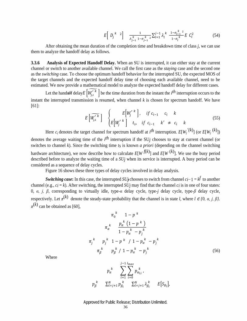
Approved for Public Release; Distribution Unlimited. 36
j,i
l
𝐸𝐸(𝐷𝐷𝑗𝑗(𝑘𝑘))2 = 1
𝛬𝛬𝑖𝑖−1(𝑘𝑘) (1−𝜎𝜎𝑖𝑖−1
(𝑘𝑘) )2∑ 𝜆𝜆𝐷𝐷
(𝑘𝑘)𝑗𝑗−1𝐷𝐷=1
(1−𝜎𝜎𝑖𝑖−1(𝑘𝑘) )2
1−𝜎𝜎𝑖𝑖(𝑘𝑘) 𝐸𝐸[𝐶𝐶𝐷𝐷2] (54)
After obtaining the mean duration of the completion time and breakdown time of class j, we can use them to analyze the handoff delay as follows. 3.3.6 Analysis of Expected Handoff Delay. When an SU is interrupted, it can either stay at the current channel or switch to another available channel. We call the first case as the staying case and the second one as the switching case. To choose the optimum handoff behavior for the interrupted SU, the expected MOS of the target channels and the expected handoff delay time of choosing each available channel, need to be estimated. We now provide a mathematical model to analyze the expected handoff delay for different cases.
Let the handoff delay𝐸𝐸 𝑊𝑊𝚥𝚥,𝚤𝚤′(𝑘𝑘) be the time duration from the instant the ith interruption occurs to the
instant the interrupted transmission is resumed, when channel k is chosen for spectrum handoff. We have [61]:
𝐸𝐸 𝑊𝑊𝚥𝚥,𝚤𝚤′(𝑘𝑘) =
𝐸𝐸𝑊𝑊𝑗𝑗′(𝑘𝑘) , 𝑖𝑖𝑓𝑓 𝑐𝑐𝑗𝑗−1 = 𝑐𝑐𝑗𝑗 = 𝑘𝑘
𝐸𝐸𝑊𝑊𝑗𝑗′(𝑘𝑘) + 𝑡𝑡𝑠𝑠, 𝑖𝑖𝑓𝑓(𝑐𝑐𝑗𝑗−1 = 𝑘𝑘′) ≠ (𝑐𝑐𝑗𝑗 = 𝑘𝑘)
(55)
Here ci denotes the target channel for spectrum handoff at ith interruption. E[Wj’(k)] (or E[Wj (k)])
denotes the average waiting time of the ith interruption if the SUj chooses to stay at current channel (or switches to channel k). Since the switching time ts is known a priori (depending on the channel switching
hardware architecture), we now describe how to calculate E[W f(k)] and E[W (k)]. We use the busy period described before to analyze the waiting time of a SUj when its service is interrupted. A busy period can be considered as a sequence of delay cycles. Figure 16 shows these three types of delay cycles involved in delay analysis.
Switching case: In this case, the interrupted SUj chooses to switch from channel ci−1 = kf to another channel (e.g., ci = k). After switching, the interrupted SUj may find that the channel ci is in one of four states: 0, α, j, β, corresponding to virtually idle, type-α delay cycle, type-j delay cycle, type-β delay cycle, respectively. Let π(k) denote the steady-state probability that the channel is in state l, where l ∈ 0, α, j, β. π(k) can be obtained as [60],
𝜋𝜋0(𝑘𝑘) = 1 − 𝑝𝑝(𝑘𝑘)
𝜋𝜋𝛼𝛼(𝑘𝑘) =
𝑝𝑝𝛼𝛼(𝑘𝑘)1 − 𝑝𝑝(𝑘𝑘)
1 − 𝑝𝑝𝛼𝛼(𝑘𝑘) − 𝑝𝑝𝑗𝑗
(𝑘𝑘)
𝜋𝜋𝑗𝑗(𝑘𝑘) = 𝑝𝑝𝑗𝑗
(𝑘𝑘)(1 − 𝑝𝑝(𝑘𝑘))/(1 − 𝑝𝑝𝛼𝛼(𝑘𝑘) − 𝑝𝑝𝑗𝑗
(𝑘𝑘))
𝜋𝜋𝛽𝛽(𝑘𝑘) = 𝑝𝑝𝛽𝛽
(𝑘𝑘)/(1 − 𝑝𝑝𝛼𝛼(𝑘𝑘) − 𝑝𝑝𝑗𝑗
(𝑘𝑘)) (56) Where
𝑝𝑝𝛼𝛼(𝑘𝑘) = 𝑝𝑝𝛼𝛼𝑖𝑖,𝑖𝑖
(𝑘𝑘)𝐼𝐼𝑚𝑚𝑖𝑖𝑥𝑥
𝑗𝑗=0
𝑗𝑗−1
𝐷𝐷=1
,
𝑝𝑝𝛽𝛽(𝑘𝑘) = ∑ 𝑝𝑝𝛽𝛽𝑖𝑖
(𝑘𝑘) = ∑ 𝜆𝜆𝛽𝛽𝑖𝑖(𝑘𝑘) = 𝐸𝐸𝑆𝑆𝐵𝐵𝑖𝑖,
𝑁𝑁𝐷𝐷=𝑗𝑗+1
𝑁𝑁𝐷𝐷=𝑗𝑗+1
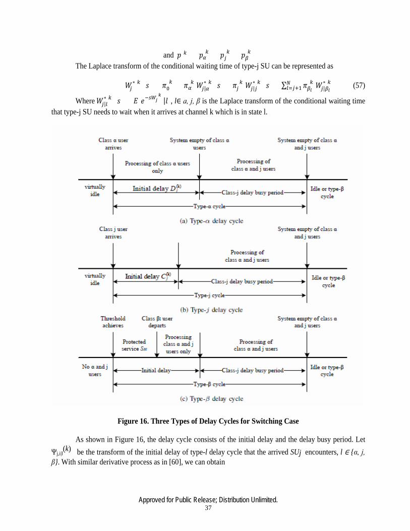
Approved for Public Release; Distribution Unlimited. 37
and 𝑝𝑝(𝑘𝑘) = 𝑝𝑝𝛼𝛼(𝑘𝑘) + 𝑝𝑝𝑗𝑗
(𝑘𝑘) + 𝑝𝑝𝛽𝛽(𝑘𝑘)
The Laplace transform of the conditional waiting time of type-j SU can be represented as
𝑊𝑊𝑗𝑗∗(𝑘𝑘)(𝑠𝑠) = 𝜋𝜋0
(𝑘𝑘) + 𝜋𝜋𝛼𝛼(𝑘𝑘)𝑊𝑊𝑗𝑗|𝛼𝛼
∗(𝑘𝑘)(𝑠𝑠) + 𝜋𝜋𝑗𝑗(𝑘𝑘)𝑊𝑊𝑗𝑗|𝑗𝑗
∗(𝑘𝑘)(𝑠𝑠) + ∑ 𝜋𝜋𝛽𝛽𝑖𝑖(𝑘𝑘)𝑊𝑊𝑗𝑗|𝛽𝛽𝑖𝑖
∗(𝑘𝑘)𝑁𝑁𝐷𝐷=𝑗𝑗+1 (57)
Where 𝑊𝑊𝑗𝑗|𝐷𝐷∗(𝑘𝑘)(𝑠𝑠) = 𝐸𝐸[𝑒𝑒−𝑠𝑠𝑊𝑊𝑖𝑖
(𝑘𝑘)|𝑙𝑙], l∈ a, j, β is the Laplace transform of the conditional waiting time
that type-j SU needs to wait when it arrives at channel k which is in state l.
Figure 16. Three Types of Delay Cycles for Switching Case
As shown in Figure 16, the delay cycle consists of the initial delay and the delay busy period. Let Ψj,i|l
(k) be the transform of the initial delay of type-l delay cycle that the arrived SUj encounters, l ∈ α, j,β. With similar derivative process as in [60], we can obtain

Approved for Public Release; Distribution Unlimited. 38
j
l
𝑊𝑊𝑗𝑗|𝐷𝐷∗(𝑘𝑘)(𝑠𝑠) =
(1−𝛹𝛹𝑖𝑖|𝑖𝑖∗(𝑘𝑘)(𝑠𝑠))
𝐸𝐸[𝑁𝑁𝑖𝑖|𝑖𝑖(𝑘𝑘)](𝑠𝑠−𝛾𝛾𝑖𝑖
(𝑘𝑘)+𝛾𝛾𝑖𝑖(𝑘𝑘)𝐶𝐶𝑖𝑖
∗(𝑘𝑘)(𝑠𝑠) (58)
where E[T (k)] represents the mean duration of type-l delay cycle. Meanwhile, as shown in the Fig. 43, we can represent the Laplace transform of the initial delay of type-α and type-j delay cycle as
𝛹𝛹𝑗𝑗|𝛼𝛼∗(𝑘𝑘)(𝑠𝑠) = 𝐷𝐷𝑗𝑗
∗(𝑘𝑘)(𝑠𝑠) 𝛹𝛹𝑗𝑗|𝑗𝑗∗(𝑘𝑘)(𝑠𝑠) = 𝐶𝐶𝑗𝑗
∗(𝑘𝑘)(𝑠𝑠) (59)
Moreover, we use γ∗(k) to denote the rate at which type-l delay cycles are encountered by SUj . Type-α or type-j delay cycle commences only when class α or class j user enters the channel in its virtually idle state. Thus we can obtain 𝛾𝛾𝛼𝛼
∗(𝑘𝑘) = 𝛬𝛬𝑗𝑗−1(𝑘𝑘) 𝜋𝜋0
(𝑘𝑘) and 𝜆𝜆 𝑗𝑗∗(𝑘𝑘) = 𝛾𝛾𝑗𝑗
(𝑘𝑘)𝜋𝜋0(𝑘𝑘). Meanwhile, we have 𝜋𝜋𝛼𝛼
(𝑘𝑘) = 𝜆𝜆 𝛼𝛼∗(𝑘𝑘)𝐸𝐸𝑘𝑘𝑗𝑗|𝜆𝜆
(𝑘𝑘)
and 𝜋𝜋𝑗𝑗(𝑘𝑘) = 𝜆𝜆 𝑗𝑗
∗(𝑘𝑘)𝐸𝐸𝑘𝑘𝑗𝑗|𝑗𝑗(𝑘𝑘). Substituting these variables and (58), (59) into (57), we can get 𝑊𝑊𝑗𝑗
∗(𝑘𝑘)(𝑠𝑠) as shown in (60). 𝑊𝑊𝑗𝑗
∗(𝑘𝑘)(𝑠𝑠)
=(1 − 𝑝𝑝𝛼𝛼
(𝑘𝑘) − 𝑝𝑝𝑗𝑗(𝑘𝑘) − ∑ 𝜆𝜆𝛽𝛽𝑖𝑖
(𝑘𝑘)𝐸𝐸𝑆𝑆𝐵𝐵𝑖𝑖) 𝑠𝑠 + 𝛬𝛬𝑗𝑗−1(𝑘𝑘) − 𝛬𝛬𝑗𝑗−1
(𝑘𝑘) 𝐷𝐷𝑗𝑗∗(𝑘𝑘)(𝑠𝑠) + ∑ 𝜆𝜆𝛽𝛽𝑖𝑖
∗(𝑘𝑘)(1 − 𝛹𝛹𝛽𝛽𝑖𝑖∗(𝑘𝑘)(𝑠𝑠)) 𝑁𝑁
𝐷𝐷=𝑗𝑗+1 𝑁𝑁𝐷𝐷=𝑗𝑗+1
𝑠𝑠 + 𝛾𝛾𝑗𝑗(𝑘𝑘) − 𝛾𝛾𝑗𝑗
(𝑘𝑘)𝐶𝐶𝑗𝑗∗(𝑘𝑘)(𝑠𝑠)
(60)
In our work, we compare the elapsed service time of SUl, l ∈ j + 1, ..., N , with the predefined threshold τl for our preemptive discretion rule. If the elapsed service time is less than τl, a high-priority user can interrupt the service of class l user. Let Fl(t) = Pr(Sl ≤ t) denote the CDF of the service time of type-l user. Type-l user cannot be preempted by users with a higher priority, if its elapsed service time is larger than τl. In this case, it will initiate a type-β delay cycle. Thus, we have 𝜆𝜆 𝐵𝐵𝑖𝑖
∗(𝑘𝑘) = 𝜆𝜆 𝐷𝐷(𝑘𝑘)(1 − 𝐶𝐶𝐷𝐷(𝜏𝜏𝐷𝐷)).
Moreover, in a type-β delay cycle, other SUs cannot interrupt the service of current low-priority SU. However, a PU can interrupt the service of any SU because PUs have the absolute preemptive control over the licensed channel. A type-β delay cycle can be considered as completed only when all type-α and type-j users arrive during the protective nonpreemptive duration of the serving SU. The busy period of type-α and type-j users which arrive during the protective nonpreemptive region of SUj , can be denoted as the breakdown
time D(k). Thus, we obtain 𝛹𝛹𝑗𝑗|𝐵𝐵𝑖𝑖∗(𝑘𝑘)(𝑠𝑠) = Ф𝑆𝑆𝐵𝐵𝑖𝑖
𝑠𝑠 + 𝛬𝛬𝑗𝑗−1(𝑘𝑘) − 𝛬𝛬𝑗𝑗−1
(𝑘𝑘) 𝐷𝐷𝑗𝑗∗(𝑘𝑘)(𝑠𝑠) (61)
Substituting (61) into (60), we obtain the final Laplace transform associated with the waiting time of class j user as shown in (62).
𝑊𝑊𝑗𝑗∗(𝑘𝑘)(𝑠𝑠) =
(1−𝑝𝑝𝛼𝛼(𝑘𝑘)−𝑝𝑝𝑖𝑖
(𝑘𝑘)−∑ 𝜆𝜆𝛽𝛽𝑖𝑖(𝑘𝑘)𝐸𝐸𝑆𝑆𝐵𝐵𝑖𝑖)𝑠𝑠+𝛬𝛬𝑖𝑖−1
(𝑘𝑘) −𝛾𝛾𝑖𝑖−1(𝑘𝑘) 𝐷𝐷𝑖𝑖
∗(𝑘𝑘)(𝑠𝑠)𝑁𝑁𝑖𝑖=𝑖𝑖+1
𝑠𝑠+𝛾𝛾𝑖𝑖(𝑘𝑘)−𝛾𝛾𝑖𝑖
(𝑘𝑘)𝐶𝐶𝑖𝑖∗(𝑘𝑘)(𝑠𝑠)
+∑ 𝜆𝜆𝛽𝛽𝑖𝑖
(𝑘𝑘)(1−Ф𝑆𝑆𝐵𝐵𝑖𝑖𝑁𝑁𝑖𝑖=𝑖𝑖+1 𝑠𝑠+𝛬𝛬𝑖𝑖−1
(𝑘𝑘) −𝛬𝛬𝑖𝑖−1(𝑘𝑘) 𝐷𝐷𝑖𝑖
∗(𝑘𝑘)(𝑠𝑠))
𝑠𝑠+𝛾𝛾𝑖𝑖(𝑘𝑘)−𝛾𝛾𝑖𝑖
(𝑘𝑘)𝐶𝐶𝑖𝑖∗(𝑘𝑘)(𝑠𝑠)
Taking the differentiation on (62) at s = 0, we have the expected waiting time of SUj at channel k as in (63).
(62)

Approved for Public Release; Distribution Unlimited. 39
j
𝐸𝐸𝑊𝑊𝑗𝑗(𝑘𝑘) =
1−𝑝𝑝𝛼𝛼(𝑘𝑘)−𝑝𝑝𝑖𝑖
(𝑘𝑘)1−𝑝𝑝𝛼𝛼(𝑘𝑘)
2𝛬𝛬𝑖𝑖−1
(𝑘𝑘) 𝐸𝐸(𝐷𝐷𝑖𝑖(𝑘𝑘))2+1−𝑝𝑝𝛼𝛼
(𝑘𝑘)2𝛾𝛾𝑖𝑖
(𝑘𝑘)(𝐶𝐶𝑖𝑖(𝑘𝑘))2+∑ 𝜆𝜆𝛽𝛽𝑖𝑖
∗(𝑘𝑘)𝐸𝐸[𝑆𝑆𝐵𝐵𝛽𝛽𝑖𝑖2 ]𝑁𝑁
𝑖𝑖=𝑖𝑖+1
2(1−𝑝𝑝𝛼𝛼(𝑘𝑘))(1−𝑝𝑝𝛼𝛼
(𝑘𝑘)−𝑝𝑝𝑖𝑖(𝑘𝑘))
(63)
Staying case: In this case, class k SU chooses to stay at the current operating channel, e.g. ci = ci−1 = k. Fig. 40 already shows that after being interrupted it will be pushed to the head of the queue 𝑄𝑄𝑗𝑗
(𝑘𝑘). It mustwait until the completion of the services of all type-α users in the queue or the newly arrived type-α users. Therefore, we can consider the waiting time of SUj in staying case as a type-α delay cycle, as shown in Figure 17. The interrupted SUj will be served when the system has served all class α users. Thus, we can obtain theLaplace transform of the waiting time of SUj in staying case as
𝑊𝑊𝑗𝑗∗(𝑘𝑘)(𝑠𝑠) = 𝑊𝑊𝑗𝑗−1|𝛼𝛼
∗(𝑘𝑘) (𝑠𝑠) (64)
=(1 − 𝛹𝛹𝑗𝑗−1|𝛼𝛼
∗(𝑘𝑘) (𝑠𝑠))
𝐸𝐸 𝑘𝑘𝑗𝑗−1|𝛼𝛼(𝑘𝑘) (𝑠𝑠 − 𝛾𝛾𝑗𝑗−1
(𝑘𝑘) + 𝛾𝛾𝑗𝑗−1(𝑘𝑘)𝐶𝐶𝑗𝑗−1
∗(𝑘𝑘)(𝑠𝑠))
=(1 − 𝛾𝛾𝑗𝑗−1
(𝑘𝑘)𝐸𝐸𝐶𝐶𝑗𝑗−1(𝑘𝑘))(1 − 𝐷𝐷𝑗𝑗−1|𝛼𝛼
∗(𝑘𝑘) (𝑠𝑠))
𝐸𝐸 𝐷𝐷𝑗𝑗−1(𝑘𝑘) (𝑠𝑠 − 𝛾𝛾𝑗𝑗−1
(𝑘𝑘) + 𝛾𝛾𝑗𝑗−1(𝑘𝑘)𝐶𝐶𝑗𝑗−1
∗(𝑘𝑘)(𝑠𝑠))
Figure 17. The Delay Cycle for Staying Case
3.3.7 Analysis of Expected Delivery Time
The expected delivery time of an SU connection, which experiences n interruptions during transmission, consists of the expected delays caused by interruptions and its service time. Since the service time of SU connections is assumed to be known, we only need to estimate its expected delay for its expected delivery time. When i > Imax, we drop the packet. This results in 𝑊𝑊𝑗𝑗,𝑗𝑗
′(𝑘𝑘) = 0. The probability that the type-(j,i) SU connection will be interrupted is 𝑃𝑃𝑗𝑗,𝑗𝑗
(𝑘𝑘) = 𝜆𝜆𝑝𝑝(𝑘𝑘)𝐸𝐸[𝑆𝑆𝑗𝑗,𝑗𝑗+1
(𝑘𝑘) ][16]. Thus, the expected delay of an SU connection with priority j can be derived as
𝐸𝐸𝐷𝐷𝑒𝑒𝑙𝑙𝑎𝑎𝑦𝑦𝑗𝑗 = ∑ 𝑖𝑖𝑃𝑃𝑗𝑗,𝑗𝑗(𝑘𝑘)𝐸𝐸[𝑊𝑊𝑗𝑗,𝑗𝑗
′(𝑘𝑘)]𝐼𝐼𝑚𝑚𝑖𝑖𝑥𝑥𝑗𝑗=0 (65)

Approved for Public Release; Distribution Unlimited. 40
j
j
j,i
j,i j
where 𝐸𝐸[𝑊𝑊𝑗𝑗,𝑗𝑗′(𝑘𝑘)] is the handoff delay describes in (55).
3.3.8 Multi-Teacher Transfer Learning for Handoff Control
3.3.8.1 QoE-Driven, RL-based Spectrum Handoff. Before describing the MAL model, we discuss the following two aspects which serve as the basis of the MAL-based handoff control: (1) QoE-driven handoff, which is more important to multimedia transmission than the delay-based handoff (i.e. only use queueing delay to determine handoff). (2) RL-based handoff, which will be extended to the MAL-based handoff. The RL-based handoff is also a necessary step for an SU to become a ‘teacher’, since any new SU that cannot find a suitable teacher should learn to adapt to the complex CRN environment by itself. Our previous work [15], [20] has covered those aspects. We briefly summarize them here for the readers’ convenience.
We denote the PER of channel k for SUj as P ERj(k). Let Delayj,i be the delay of a SUj connection
due to the first (i − 1) interruptions. An SUj packet will be dropped when its delay exceeds the delay deadline
dj . Let P DRj(k) (packet dropping rate) be the probability of packet being dropped during the ith interruption.
It equals to the probability of E[Dj,ik ] being larger than dj − Delayj,i. Both PER and PDR have been derivedin our previous work [15].
Let T P ERj(k) (total packet error rate) be the estimated total PER of channel k for SUj at its ith
interruption. Assuming PER and PDR are independent of each other, we have T P ERj(k) = P ERj
(k) + PDRj
(k) − P ERj(k) · P DRj
(k). Using the QoE model derived in [62], the expected MOS (mean opinion score)for SUj choosing channel k for its ith interruption, M OS(k), can be represented as a function of the senderbitrate (SBR), frame rate (FR) and the 𝑘𝑘𝑃𝑃𝐸𝐸𝑅𝑅𝑗𝑗
(𝑘𝑘).
𝐻𝐻𝑀𝑀𝑆𝑆𝑗𝑗,𝑗𝑗(𝑘𝑘) = 𝜏𝜏1+𝜏𝜏2𝑇𝑇𝐹𝐹+𝜏𝜏3ln (𝑆𝑆𝐵𝐵𝐹𝐹)
1+𝜏𝜏4𝑁𝑁𝑃𝑃𝐸𝐸𝐹𝐹𝑖𝑖(𝑘𝑘)+𝜏𝜏5(𝑁𝑁𝑃𝑃𝐸𝐸𝐹𝐹𝑖𝑖
(𝑘𝑘))2 (66)
The coefficients 𝜏𝜏1, 𝜏𝜏2, 𝜏𝜏3 , 𝜏𝜏4, 𝜏𝜏5 can be obtained by a linear regression analysis [62]. Next, we can use RL-based model, with MOS-based reward function, to define an optimal spectrum
handoff strategy. The RL model could be based on our previous work [15], except that we have to consider the queueing delay differences for 3 types of SUs described in the previous section.
3.3.8.2 Multi-Teacher Knowledge Transfer for Intelligent Spectrum Handoff. Due to the complex and dynamic nature of the spectrum conditions in CRNs, the learning process of RL could be slow, especially in the startup phase or when an SU goes through a new radio environment. The AL (Apprenticeship Learning) can be used to make the apprentice SU perform as well as the expert SU by learning from the expert knowledge [63], [64]. Unlike our previous work that uses a single-teacher model [20], here we use MAL framework, which allows an apprentice SU to learn from multiple experts simultaneously. Choosing multiple teachers helps to avoid the biased knowledge of a particular SU teacher.
Multiple teachers could teach the student SU from different aspects. For example, a SU may find a teacher with the matching link channel statistics to learn how to choose the proper sending rate based on the channel statistics. It may find another teacher with the matching QoS statistics to learn how to choose a QoS-oriented routing path from it. To find a suitable teacher, we need to define the similarity index (i.e., feature distance) between any two SUs. As shown in Figure 18, we consider a high- dimensional signals consisting of multiple types of network parameters such as: (1) channel statistics such as BER, SNR, etc., SU statistics such as node mobility, modulation mode, etc., (3) QoS statistics such as end-to-end delay, jitter, etc. The SU

Approved for Public Release; Distribution Unlimited. 41
that has the biggest similarity index in any of those parameters, can be selected as a teacher. Such a similarity index should be based on the statistical distance between two manifold signals.
Typically geodesic distance is used to measure the shortest length between any two manifold points. However, such distance is difficult to calculate. Therefore, we use the Bregman Divergence (BD) [65] to replace the geodestic distance. The BD between two manifold points p and q, denoted as D(p, q), is associated with a generator function Φ(),
𝐷𝐷Ф(𝑝𝑝, 𝑞𝑞) = Ф(𝑝𝑝) − ⟨Ф(𝑞𝑞) − 𝛻𝛻Ф(𝑞𝑞), 𝑝𝑝 − 𝑞𝑞⟩ (67) where 𝛻𝛻Ф = [𝜕𝜕Ф
𝜕𝜕𝑥𝑥1, 𝜕𝜕Ф𝜕𝜕𝑥𝑥2
, … ] is the inner product operation. We then define the concept of Bregman ball, which has a center µk , and a radius Rk . If any manifold point Xt is inside this ball, it has a strong statistical similarity between itself and the center µk . That is:
𝐵𝐵(µ𝑘𝑘 ,𝑅𝑅𝑘𝑘) = 𝑋𝑋𝑡𝑡 ∈ 𝑋𝑋:𝐷𝐷Ф(𝑋𝑋𝑡𝑡 ,𝑚𝑚µ𝑘𝑘) ≤ 𝑅𝑅𝑘𝑘 (68)
Figure 18. Information Geometry Based Node-to-Node Teaching
In the multi-teacher model, we denote the student SU as SUa, and its state feature vector over states as φ(s). We assume that n teachers (SUe1 , · · · , SUen ) are selected. We weigh the knowledge from the teachers by the normalized similarity indexes between the student and the teacher in the feature space, sim(SUa, SUe1 ), · · · , sim(SUa, SUen ), which are derived from their symmetric Bregman divergences. The similarity scores are normalized such that the summation is 1. The expected MOS of the apprentice SU, 𝐻𝐻𝑀𝑀𝑆𝑆𝑗𝑗,𝑗𝑗
(𝑘𝑘)(𝜙𝜙(𝑠𝑠𝑗𝑗)), is a combination of the experts’ MOS, 𝐻𝐻𝑀𝑀𝑆𝑆𝑆𝑆𝑆𝑆𝑖𝑖𝑖𝑖 ,𝑗𝑗,𝑗𝑗(𝑘𝑘) (𝜙𝜙(𝑠𝑠𝑗𝑗)), and the self-estimated MOS,
𝐻𝐻𝑀𝑀𝑆𝑆𝑆𝑆𝑆𝑆𝛼𝛼,𝑗𝑗,𝑗𝑗(𝑘𝑘) (𝜙𝜙(𝑠𝑠𝑗𝑗)), with a decreasing effect from the teachers’ MOS along time, as follows:

Approved for Public Release; Distribution Unlimited. 42
𝐻𝐻𝑀𝑀𝑆𝑆𝑗𝑗 ,𝑗𝑗(𝑘𝑘)𝜙𝜙(𝑠𝑠𝑗𝑗) (69)
= 𝛾𝛾𝑗𝑗[ 𝑠𝑠𝑖𝑖𝑚𝑚(𝑆𝑆𝐶𝐶𝑎𝑎 , 𝑆𝑆𝐶𝐶𝐷𝐷1) ∙ 𝐻𝐻𝑀𝑀𝑆𝑆𝑆𝑆𝑆𝑆𝑖𝑖𝑖𝑖 ,𝑗𝑗,𝑗𝑗(𝑘𝑘) (𝜙𝜙(𝑠𝑠𝑗𝑗)) ] + (1 − 𝛾𝛾𝑗𝑗)𝐻𝐻𝑀𝑀𝑆𝑆𝑆𝑆𝑆𝑆𝛼𝛼,𝑗𝑗,𝑗𝑗
(𝑘𝑘) (𝜙𝜙(𝑠𝑠𝑗𝑗))𝑛𝑛
𝐷𝐷=1
where 𝛾𝛾 < 1 is the multiplication ratio that decreases sequentially to indicate the weaker and weaker effect of experts’ MOS expectation. The Q-values are updated for a given connection during its multiple interruptions:
𝑄𝑄(𝑠𝑠, 𝑎𝑎) = (1 − 𝛼𝛼)𝑄𝑄(𝑠𝑠, 𝑎𝑎) + 𝛼𝛼𝐸𝐸𝐻𝐻𝑀𝑀𝑆𝑆𝑗𝑗,𝑗𝑗+1𝛾𝛾 𝑄𝑄(𝑠𝑠′, 𝑎𝑎′);𝑎𝑎′∈𝐴𝐴𝑚𝑚𝑎𝑎𝑥𝑥 (70)
𝑄𝑄(𝑠𝑠, 𝑎𝑎) = 𝜂𝜂𝑗𝑗 𝑄𝑄𝑆𝑆𝑆𝑆𝑖𝑖1
𝑛𝑛
𝐷𝐷=1
(𝑠𝑠, 𝑎𝑎) + 1 − 𝜂𝜂𝑗𝑗𝑄𝑄𝑆𝑆𝑆𝑆𝑖𝑖(𝑠𝑠, 𝑎𝑎)
where η < 1 is the multiplication ratio.
The system diagram of the MAL-based handoff is shown in Figure 19. If the expected MOS is less than a predefined threshold, it will perform MAL-based QoE-driven spectrum handoff to learn from its expert SUs. The handoff operations are described in Algorithm 3.
Figure 19. Multi-Teacher Based Spectrum Handoff. (Adapted From Our Single-Teacher Mode in [20]

Approved for Public Release; Distribution Unlimited. 43
Algorithm 3. MAL-Based Spectrum Handoff
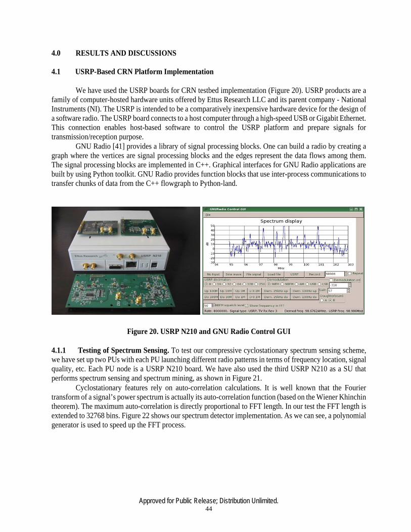
Approved for Public Release; Distribution Unlimited. 44
4.0 RESULTS AND DISCUSSIONS 4.1 USRP-Based CRN Platform Implementation We have used the USRP boards for CRN testbed implementation (Figure 20). USRP products are a family of computer-hosted hardware units offered by Ettus Research LLC and its parent company - National Instruments (NI). The USRP is intended to be a comparatively inexpensive hardware device for the design of a software radio. The USRP board connects to a host computer through a high-speed USB or Gigabit Ethernet. This connection enables host-based software to control the USRP platform and prepare signals for transmission/reception purpose. GNU Radio [41] provides a library of signal processing blocks. One can build a radio by creating a graph where the vertices are signal processing blocks and the edges represent the data flows among them. The signal processing blocks are implemented in C++. Graphical interfaces for GNU Radio applications are built by using Python toolkit. GNU Radio provides function blocks that use inter-process communications to transfer chunks of data from the C++ flowgraph to Python-land.
Figure 20. USRP N210 and GNU Radio Control GUI 4.1.1 Testing of Spectrum Sensing. To test our compressive cyclostationary spectrum sensing scheme, we have set up two PUs with each PU launching different radio patterns in terms of frequency location, signal quality, etc. Each PU node is a USRP N210 board. We have also used the third USRP N210 as a SU that performs spectrum sensing and spectrum mining, as shown in Figure 21. Cyclostationary features rely on auto-correlation calculations. It is well known that the Fourier transform of a signal’s power spectrum is actually its auto-correlation function (based on the Wiener Khinchin theorem). The maximum auto-correlation is directly proportional to FFT length. In our test the FFT length is extended to 32768 bins. Figure 22 shows our spectrum detector implementation. As we can see, a polynomial generator is used to speed up the FFT process.
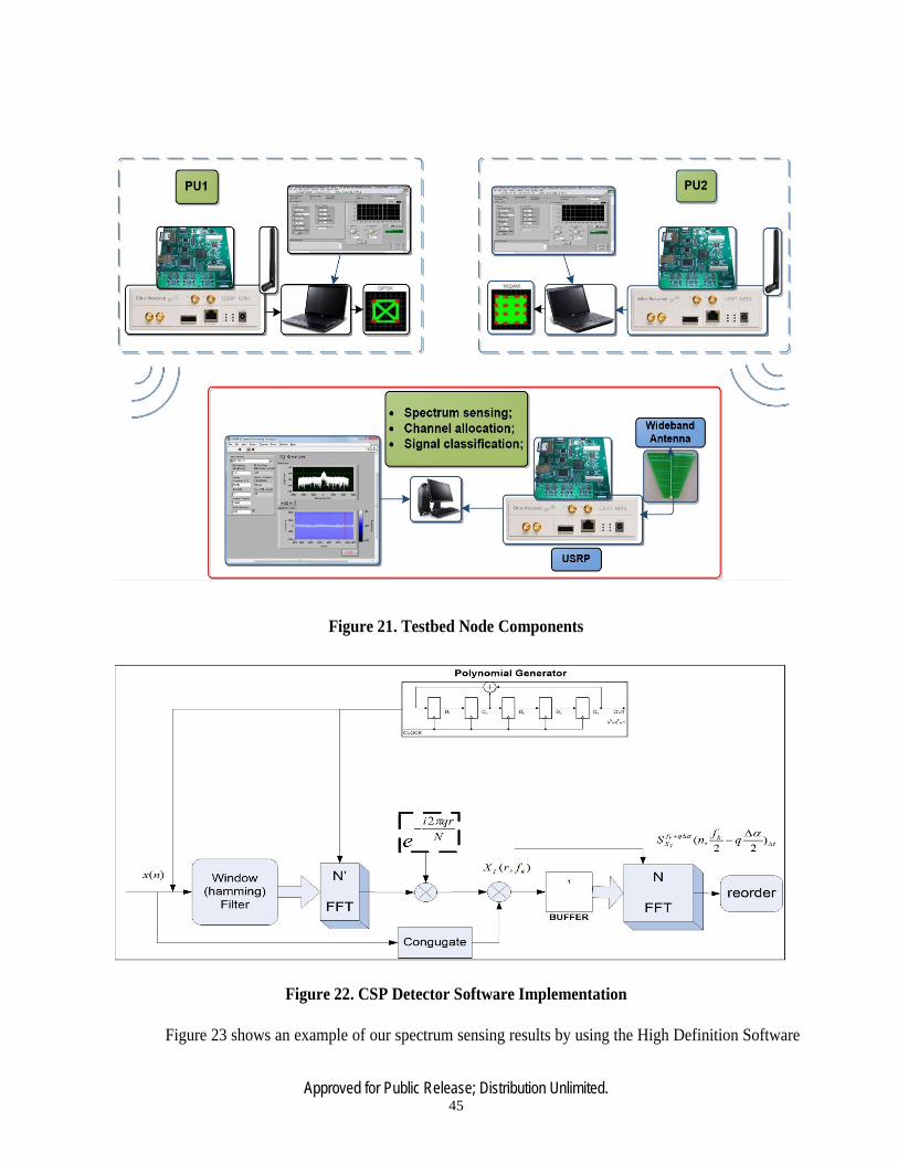
Approved for Public Release; Distribution Unlimited. 45
Figure 21. Testbed Node Components
Figure 22. CSP Detector Software Implementation
Figure 23 shows an example of our spectrum sensing results by using the High Definition Software
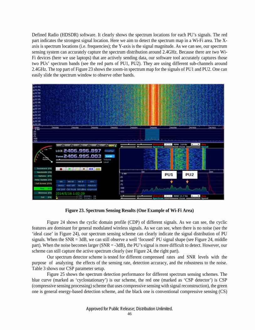
Approved for Public Release; Distribution Unlimited. 46
Defined Radio (HDSDR) software. It clearly shows the spectrum locations for each PU’s signals. The red part indicates the strongest signal location. Here we aim to detect the spectrum map in a Wi-Fi area. The X-axis is spectrum locations (i.e. frequencies); the Y-axis is the signal magnitude. As we can see, our spectrum sensing system can accurately capture the spectrum distribution around 2.4GHz. Because there are two Wi-Fi devices (here we use laptops) that are actively sending data, our software tool accurately captures those two PUs’ spectrum bands (see the red parts of PU1, PU2). They are using different sub-channels around 2.4GHz. The top part of Figure 23 shows the zoom-in spectrum map for the signals of PU1 and PU2. One can easily slide the spectrum window to observe other bands.
Figure 23. Spectrum Sensing Results (One Example of Wi-Fi Area) Figure 24 shows the cyclic domain profile (CDP) of different signals. As we can see, the cyclic features are dominant for general modulated wireless signals. As we can see, when there is no noise (see the ‘ideal case’ in Figure 24), our spectrum sensing scheme can clearly indicate the signal distribution of PU signals. When the SNR = 3dB, we can still observe a well ‘focused’ PU signal shape (see Figure 24, middle part). When the noise becomes larger (SNR = -3dB), the PU’s signal is more difficult to detect. However, our scheme can still capture the active spectrum clearly (see Figure 24, the right part). Our spectrum detector scheme is tested for different compressed rates and SNR levels with the purpose of analyzing the effects of the sensing rate, detection accuracy, and the robustness to the noise. Table 3 shows our CSP parameter setup. Figure 25 shows the spectrum detection performance for different spectrum sensing schemes. The blue curve (marked as ‘cyclostationary’) is our scheme, the red one (marked as ‘CSP detector’) is CSP (compressive sensing processing) scheme that uses compressive sensing with signal reconstruction), the green one is general energy-based detection scheme, and the black one is conventional compressive sensing (CS)

Approved for Public Release; Distribution Unlimited. 47
scheme without spectrum mining. As we can see, our scheme has the highest spectrum detection accuracy due to the use of both CS and non-reconstruction spectrum mining algorithm.
Figure 24. Cyclic Features for Different Signals at Different SNRs
TABLE 3. Experiment Parameters in Compressive Spectrum Sensing
4.1.2 Testing of Spectrum Mining
As explained before, spectrum mining can be used to classify the spectrum bands into different categories based on their common features. As shown in Figure 26, the spectrum classification errors quickly approach to zero in high SNR environment. Using SNR=25dB as an example, the classification error is almost zero when the compression ratio is 20%, which means that 20% of the spectrum sensing energy could be saved since only 20% spectrum samples are needed for spectrum mining.

Approved for Public Release; Distribution Unlimited. 48
Figures 27 and 28 show the spectrum mining results after using SVM-based clustering algorithms. As we can see from Figure 27, before we apply the cyclic features in the clustering algorithm, the signal measurements are sensitive to the noise and become difficult to classify for the low-SNR conditions (we can see that all red and blue points are mixed together in Figure 27). While in Figure 28, we have introduced the cyclic feature measurements, and all signal measurements can be well separated. This is because that the cyclic features can be used to easily distinguish among different signals.
Figure 25. Performance of Spectrum Detection Schemes
Figure 26. Spectrum Classification Performance (X-axis: compression ratio; Y-axis: classification
error probability)

Approved for Public Release; Distribution Unlimited. 49
Figure 27. SVM-based Pattern Clustering for Non-Cyclic Domain (X-axis: normalized signal position in X direction; Y-axis: Normalized signal position in Y-direction). Red points: BPSK signals; Blue
points: QPSK signals
Figure 28. SVM-based Pattern Clustering for Compressive Cyclic Domain (X-axis: Normalized signal position in X direction; Y-axis: Normalized signal position in Y-direction). Red points: BPSK signals;
Blue points: QPSK signals

Approved for Public Release; Distribution Unlimited. 50
4.1.3 Testing of Spectrum Handoff. In this test, we use a USRP node as an interference source (see Figure 29). When the receiver detects the interference, it sends a message to the sender. Then both the sender and receiver will switch to a new channel. We use a video transmission application to test the channel switching accuracy and the response time for our intelligent spectrum handoff scheme. The sender captures the real-time video with a built-in camera in the host computer. And the jamming node launches the video signals from its built-in camera (as the jamming signals). The experiment parameters on the sender side are shown in Table 4.
Figure 29. Setup of Spectrum Handoff Test
TABLE 4. Experiment Parameters in Intelligent Spectrum Handoff (Sender Side)
We have used multi-thread programming for spectrum handoff control. A thread of execution is the smallest sequence of programmed instructions that can be managed independently by a scheduler. The thread is a component of the process. Multiple threads can co-exist within the same process, execute concurrently, and share the resources such as the memory. In particular, the threads of a process share their instructions (executable codes) and contexts (its variables). In GNU Radio programming, each action of the USRP board is controlled by one thread. In the thread, one can build a radio chain by defining a flowgraph. The connection function specifies how the output stream of a processing block connects to the input stream of the downstream blocks. The system then automatically builds the flowgraph. The details of this process are hidden from the user.
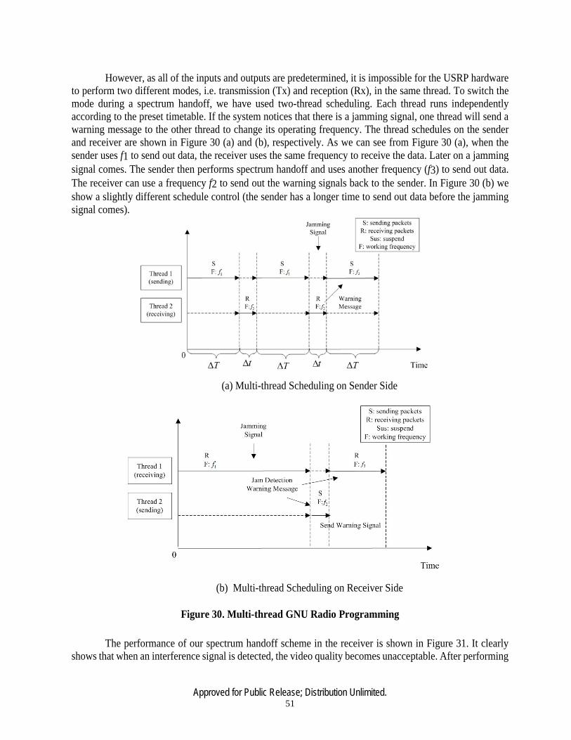
Approved for Public Release; Distribution Unlimited. 51
However, as all of the inputs and outputs are predetermined, it is impossible for the USRP hardware to perform two different modes, i.e. transmission (Tx) and reception (Rx), in the same thread. To switch the mode during a spectrum handoff, we have used two-thread scheduling. Each thread runs independently according to the preset timetable. If the system notices that there is a jamming signal, one thread will send a warning message to the other thread to change its operating frequency. The thread schedules on the sender and receiver are shown in Figure 30 (a) and (b), respectively. As we can see from Figure 30 (a), when the sender uses f1 to send out data, the receiver uses the same frequency to receive the data. Later on a jamming signal comes. The sender then performs spectrum handoff and uses another frequency (f3) to send out data. The receiver can use a frequency f2 to send out the warning signals back to the sender. In Figure 30 (b) we show a slightly different schedule control (the sender has a longer time to send out data before the jamming signal comes).
(a) Multi-thread Scheduling on Sender Side
(b) Multi-thread Scheduling on Receiver Side
Figure 30. Multi-thread GNU Radio Programming
The performance of our spectrum handoff scheme in the receiver is shown in Figure 31. It clearly shows that when an interference signal is detected, the video quality becomes unacceptable. After performing

Approved for Public Release; Distribution Unlimited. 52
the spectrum handoff, the video quality becomes good again. (1) Before jamming (2) After jamming (3) Recovered signals
Figure 31. Video Quality (Before/After Spectrum Handoff)
4.1.4 Testing of Raptor Codes. We have also evaluated the performance of video transmission over CRN with Raptor codes. In the first experiment, the raw video source is encoded by H.264/AVC encoder, and then followed by Raptor codes at the Application layer. After that the encoded Raptor packets are packed into UDP packets, modulated and transmitted over the wireless channel. In the second experiment, the raw video source is encoded by H.264/AVC only without using Raptor codes. From Figure 32, we can see that the video quality with Raptor codes is much better than the one without using Raptor codes. The experiment parameters (on the sender) are shown in Table 5.
Figure 32. One Frame of the Received Video. (Left) Video Transmission without Raptor Codes;
(Right) Video Transmission with Raptor Codes.

Approved for Public Release; Distribution Unlimited. 53
TABLE 5. Experiment Parameters in Raptor Codes for Reliable Video Transmission (Sender Side)
4.1.5 Other Test Results
We have also built a TDMA-based MAC scheme since scheduled transmissions are popular in multimedia communications. Although many CSMA-based MAC schemes have been implemented in USRP nodes, very little work has been done on TDMA- based MAC implementation in USRP boards. Figure 33 shows our test setup. To achieve multi-video transmissions between two USRP nodes, we use a built-in camera of the host computer and a USB camera (plugged in to the computer) to capture two video streams simultaneously.
Figure 33. TDMA-based Video Communications.
The experimental parameters are listed in Table 6, and the result of the multi-video transmissions is shown in Figure 34. When the sender alternates the transmissions of two video flows (one is from the USB

Approved for Public Release; Distribution Unlimited. 54
camera, and the other one is from the built-in camera), the receiver can receive those two video flows’ packets with high video quality, based on the preset TDMA schedule
TABLE 6. Parameters in Multi-video Transmissions
(a) Sender Side (b) Receiver Ride
Figure 34. Multi-Video Transmission Test 4.2 TACT-based Spectrum Handoff: Performance Evaluation In this section we evaluate the performance of our handoff model including channel selection, decoding CDF, and enhanced TACT learning. 4.2.1 Channel Selection. We first examine our channel selection scheme (described in Section 3.2), especially the effect of two parameters: the spectrum sensing accuracy, MA, and is the channel idle duration, ME . We assume that the channel idle duration follows the exponential distribution. We set up the parameters as shown in Table 7. Then we estimate the state transition sequences and the corresponding observation sequences. Additionally, we consider multiple available channels and rank the m channels in the decreasing order based on the estimated CUF. We consider N = 10 PUs, with each PU possessing one primary channel.
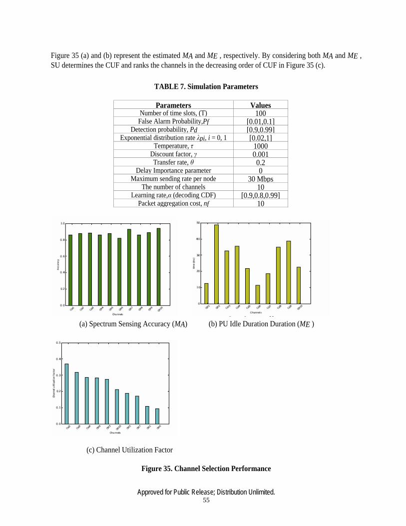
Approved for Public Release; Distribution Unlimited. 55
Figure 35 (a) and (b) represent the estimated MA and ME , respectively. By considering both MA and ME , SU determines the CUF and ranks the channels in the decreasing order of CUF in Figure 35 (c).
TABLE 7. Simulation Parameters
Parameters ValuesNumber of time slots, (T) 100
False Alarm Probability,Pf [0.01,0.1]Detection probability, Pd [0.9,0.99]
Exponential distribution rate λpi, i = 0, 1 [0.02,1]Temperature, τ 1000
Discount factor, γ 0.001Transfer rate, θ 0.2
Delay Importance parameter 0Maximum sending rate per node 30 Mbps
The number of channels 10Learning rate,α (decoding CDF) [0.9,0.8,0.99]
Packet aggregation cost, nf 10
(a) Spectrum Sensing Accuracy (MA) (b) PU Idle Duration Duration (ME )
(c) Channel Utilization Factor
Figure 35. Channel Selection Performance

Approved for Public Release; Distribution Unlimited. 56
Figure 36 depicts the system throughput achieved by our channel selection scheme for different frame durations (FDs) and PU idle durations. The BIGS in Figure 35 refers to our channel sensing scheme using the Bayesian Interference with Gibbs Sampling [7], which is one of the prominent channel sensing schemes. For comparison, we also investigate the throughput for the random channel selection (RCS) scheme. Our approach (i.e. BIGS) achieves better throughput than RCS because it selects the channels with high sensing accuracy as well as the maximum PU idle duration, whereas RCS is not only prone to missed channel detection, but also does not consider the CHT.
Figure 36. Comparison of Different Channel Selection Schemes (I)
In Figure 37, we compare our channel selection scheme with [46] and [47]. In our scheme, the SU senses the channels and ranks them based on the sensing accuracy and CHT. Similarly, authors in [47] performed the channel sensing based on the energy detection, and categorized the channels based on the CHT. In addition to this, they considered the directional antenna whereas we assumed the use of omni-directional antenna here. Since the interference level could be lower when using directional antennas as compared to omni-directional antennas, the scheme in [47] shows higher channel sensing accuracy than ours. Since the channel selection is random, in [46], the SU may select a channel with short CHT. Therefore, though its sensing accuracy is close to ours, its channel may have to perform spectrum handoff to another channel more frequently. As a result, the scheme in [46] achieves a lower throughput than our scheme. Channel selection based on the ranking is thereafter very important to achieve smooth communication and avoid the frequent spectrum handoffs.

Approved for Public Release; Distribution Unlimited. 57
Figure 37. Comparison of Different Channel Selection Schemes (II)
4.2.2 Average Queuing Delay. We compare the queuing delay of the NPRP M/G/1 model with the general queueing model in which all the applications have the same priority. we assume that the service time of SUs follows the exponential distribution, the number of channels is 10, and the maximum transmission rate of each channel is 3Mbps. Figure 38 shows that the use of user priority provides a lower delay to higher priority applications as compared to the non-prioritized model, since the idle channels are assigned based on the user priority, and the higher priority user (such as real-time video) gets more channel access opportunities, which decreases their average queuing delay, at the cost of the lower priority users which experience a longer average delay. In the case of the non-prioritization method, all the applications are given the same priority, which leads to an increase in the average delay. This is undesirable for the SUs with high delay sensitivity.
Figure 38. Average Delay for NPRP Queueing Model and Non-prioritized Model

Approved for Public Release; Distribution Unlimited. 58
4.2.3 Decoding CDF learning. Here we examine the decoding CDF over a range of symbols for different SNR values. Especially we focus on the throughput of the channel obtained by using Raptor codes. Figure 39 shows the plot of decoding CDF using Algorithm 1 for different SNR values. For higher SNR we require less number of symbols to decode a particular transmitted packet. Here the message block length k = 4; the total number of message bits n = 1024 bits; the depth B = 256 (for Spinal codes); and the packet aggregation cost nf =10. The channel is assumed to be the Rayleigh fading channel.
Using the decoding CDF, we examine the channel throughput for Raptor codes in Figure 40. For better visualization, one section of Figure 41 is zoomed in Figure 40. As mentioned before, decoding CDF enables us to find the optimal feedback strategy, i.e., when to pause for feedback and how many symbols should be transmitted before the next pause. The throughput is examined at 2.4GHz within a time range of 100 ms. We assume that the SU is moving at a speed of 10 m/s with the average link SNR of 15dB. The throughput is estimated offline using Algorithm 1 with learning rate parameter, α, set to 0.9. It can be seen that the learning rate needs not to be close to 1 to obtain a good performance. In fact, α = 0.8 performs as good as α = 0.9, whereas α = 0.99 performs worse than α = 0.8. The Raptor codes has an average throughput of half the Shannon capacity, due to the channel noise, MAC layer access collisions, and queue overflow loss.
Figure 39. Estimated CDF for Different SNR Levels
Figure 40. Throughput of Different Rateless Coding Schemes

Approved for Public Release; Distribution Unlimited. 59
Figure 41. Zoomed-in Section of Details of Figure 40
4.2.4 Effect of Traffic Load on PER and PSNR. We compare our learning-based spectrum handoff scheme (it considers the comprehensive channel metric (CSM)) and a conventional scheme that only considers the channel interference (CI) when determining spectrum handoff actions [6]. Table VIII depicts the PER. Peak SNR (PSNR) is often used to compare the signal quality when the signals have a wide dynamic range of SNR levels. It is a typical QoE metric for video application. Here we consider the following four application priorities (P 1 ∼ P 4): (1) P1 (video conference traffic) with a resolution of 640x480pixels, 10 frames per second, bit rate: 512kbps, delay bound: 500ms. The error-free PSNR of the video sequence is 31.4dB; (2) P2 (live streaming) with 1280x720pixels, 30 frames per second, 2Mbps, and delay bound: 2s, the error-free PSNR: 31.4 dB; (3) P3 (video-on-demand (pre-encoded)) with 1280x720pixels, 2Mbps, delay bound: 4s, the error-free PSNR: 34.3 dB; (4) P4 (file downloading) which does not have delay deadline.
Our results in Table 8 clearly show that our spectrum handoff scheme outperforms the CI scheme. The reason is that we have considered CSM, the priorities of different applications, node position, etc., including rateless codes. The use of decoding CDF further improves the effective channel utilization. The CI method just chooses the channel randomly. It thus experiences higher PER, and the packets may easily get dropped because of the poor channel quality and unpredictable interruptions from the PUs. Recall that in our scheme, we choose the channel with long idle duration and high throughput, which reduces the packet loss rate.
TABLE 8. PER Comparisons for Different Traffic Loads.
Figure 42 shows the effect of traffic load on video PSNR. As we can see, the PSNR decreases with the increase in the traffic load. When the traffic load is high, the packets used to wait for a longer time before

Approved for Public Release; Distribution Unlimited. 60
being transmitted. If the wait time surpasses the delay deadline, the packets get dropped, and the video quality degrades (i.e. low PSNR).
Figure 42. Effect of Traffic Load on Video PSNR for Different Spectrum Handoff Schemes Figure 43 shows the video quality comparisons for learning-based spectrum handoff and the myopic scheme. Figure 43 (d)-(f) are the zoomed-in parts of (a)-(c). As we can see, our learning-based spectrum handoff scheme achieves a better video quality at the receiver than the myopic scheme. This is because the myopic scheme only tries to maximize the short-term throughput without considering the impact of current spectrum handoff decisions on the future transmissions. Our learning-based handoff scheme aims to maximize the long-term throughput.
Figure 43. Video Effect Comparisons of Learning-based and Myopic Spectrum Decision Schemes.

Approved for Public Release; Distribution Unlimited. 61
4.2.5 TACT-enhanced Spectrum handoff. In this section, we examine the performance of our TACT-based spectrum handoff strategy. We assume that the peak sending rate of each SU is 3Mbps. All SUs adopt rateless codes, and the expert SU teaches a new SU about its transmission strategy based on the decoding-CDF profile. We examine TACT performance for the following four cases: In case 1, the newly joined SU moves slowly (static or < 5mph); In case 2, the SU moves fast (> 50mph) and experiences different channel variations; In case 3, the SU moves fast and does not use the decoding CDF for transmission control. It manually changes the symbol sending rate based on the current channel conditions; and in case 4, the SU moves fast and uses the decoding CDF. The MOS varies from 1 to 5. In general, the variation of MOS is directly proportional to PSNR.
From Figure 44 (a) (Case 1), we observe that the Q-learning based spectrum handoff outperforms the myopic approach. The reason is that Q-learning considers the future rewards (i.e., MOS). Hence, it chooses spectrum handoff actions with the best long-term throughput performance. Figure 43 (a) also shows that our TACT-based spectrum handoff slightly outperforms the Q-learning based handoff scheme since the SU can learn from the expert SU, and thus spends less time in understanding the channel dynamics. This eventually helps it to converge to a stable MDP solution more quickly.
Figure 44 (b) (Case 2) shows the result for fast moving SU. It experiences channel condition variations with time. Our TACT scheme still performs better than Q-learning scheme.
Figure 45 (a) (Case 3) depicts the case where the SU moves fast and does not use the decoding-CDF. Since the SU is moving fast, it experiences time-varying channel conditions. Once the SU attains the convergent state it achieves a high MOS value. However, it does not guarantee that the SU will stay in the optimal state throughout the entire communication process due to the varying channel conditions. Since the SU keeps transmitting at the same rate believing that the receiver is able to decode the packet, the MOS stays at a lower level (around 4.0) without much improvement.
Whereas in Figure 45 (b) (Case 4), the SU uses the decoding-CDF curve to learn the strategy of transmitting more symbols without introducing much overhead. Therefore, the SU achieves higher MOS. In both cases the MOS drops due to the change in channel condition at timeslot 7. But the use of decoding-CDF quickly helps to achieve a better MOS (i.e. MOS=4.4). Thus the link adaptation is performed using the decoding-CDF when MOS is below the threshold value due to the low channel quality (due to the mobility of SU). The MOS fluctuates because the Markov decision model is an iterative process and it needs certain time to converge to the stable state.

Approved for Public Release; Distribution Unlimited. 62
Figure 44. Learning Performance with TACT, Q-learning and Myopic Schemes

Approved for Public Release; Distribution Unlimited. 63
Figure 45. Performance Comparisons with and without Decoding CDF

Approved for Public Release; Distribution Unlimited. 64
4.3 Multi-Teacher Based Spectrum Handoff: Experimental Results In this section, we evaluate spectrum handoff scheme. As suggested by IEEE 802.22 standard [66], 10 msec per time slot is used in our experiments. Similar to the three queueing models in [13], [15], [16], we assume that the service time of PUs and SUs follow the exponential distribution. According to the property of the exponential distribution, the service time E[x] = 1/ μ, and the remaining transmission time of SUs follow the same exponential distribution after being interrupted by Pus and SUs [17]. 4.3.1 QoS-aware Spectrum Handoff Scheme. In this section, we compare our hybrid priority queueing model with three recent queueing models in [13], [15], [16]. The number of channels is M = 3, and the number of priority classes of SU connections is N = 4, and class j has a higher priority than j + 1. Here we consider the traffic delay, packet error rate, and user priority as the QoS parameters. (1) Effect of PU Traffic Load: As expected, from Figure 46 (a), we observe that, the average data delivery time gets longer with increase in the normalized PU traffic load for all SUs. In our hybrid queueing model, the SU connections with higher priorities have less average delivery time than those using the queueing models in [13], [15], [16]. Both SU1 and SU2 in the queueing model of [16] have almost the same delay. Thus the queueing model in [16] is not suitable for the applications when some SUs have more stringent delay requirement than others. Furthermore, from Figure 45 (b), the overall average delivery time across SUs of all priorities achieved by our model is much lower than the model in [13], and is comparable to the models in [15]. Although the hybrid model has about 10% performance degradation in the average delivery time compared to the model in [16], the improvement of the delay performance for higher priority SUs is significant (about 2.5x improvement for the highest priority - SU1). Since tthe higher priority SUs (such as the SUs that deliver real-time videos) demand a lower delay, our scheme can meet their delay demands, at a cost of the slight performance degradation for lower priority SUs.
(a) Average delay of SU1 through SU2
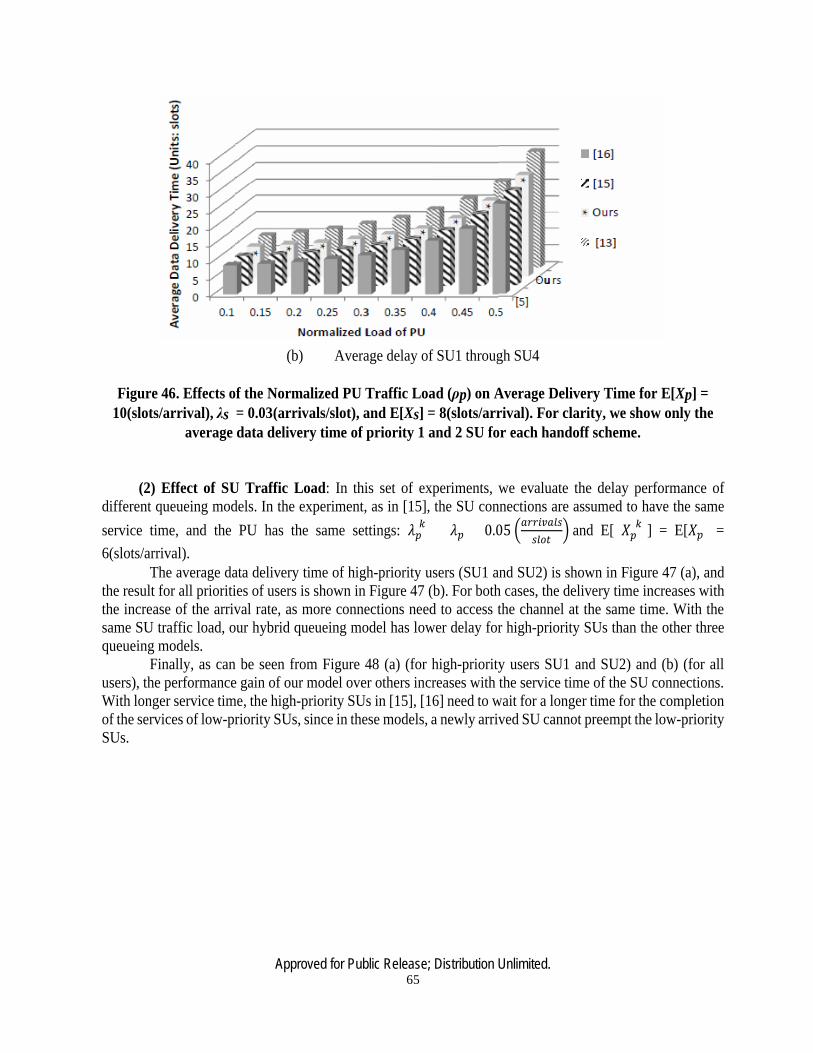
Approved for Public Release; Distribution Unlimited. 65
(b) Average delay of SU1 through SU4
Figure 46. Effects of the Normalized PU Traffic Load (ρp) on Average Delivery Time for E[Xp] = 10(slots/arrival), λs = 0.03(arrivals/slot), and E[Xs] = 8(slots/arrival). For clarity, we show only the
average data delivery time of priority 1 and 2 SU for each handoff scheme.
(2) Effect of SU Traffic Load: In this set of experiments, we evaluate the delay performance of different queueing models. In the experiment, as in [15], the SU connections are assumed to have the same service time, and the PU has the same settings: 𝜆𝜆𝑝𝑝
(𝑘𝑘) = 𝜆𝜆𝑝𝑝 = 0.05 𝑎𝑎𝑛𝑛𝑛𝑛𝑗𝑗𝑎𝑎𝑎𝑎𝐷𝐷𝑠𝑠𝑠𝑠𝐷𝐷𝑛𝑛𝑡𝑡
and E[ 𝑋𝑋𝑝𝑝(𝑘𝑘)] = E[𝑋𝑋𝑝𝑝] =
6(slots/arrival). The average data delivery time of high-priority users (SU1 and SU2) is shown in Figure 47 (a), and
the result for all priorities of users is shown in Figure 47 (b). For both cases, the delivery time increases with the increase of the arrival rate, as more connections need to access the channel at the same time. With the same SU traffic load, our hybrid queueing model has lower delay for high-priority SUs than the other three queueing models.
Finally, as can be seen from Figure 48 (a) (for high-priority users SU1 and SU2) and (b) (for all users), the performance gain of our model over others increases with the service time of the SU connections. With longer service time, the high-priority SUs in [15], [16] need to wait for a longer time for the completion of the services of low-priority SUs, since in these models, a newly arrived SU cannot preempt the low-priority SUs.
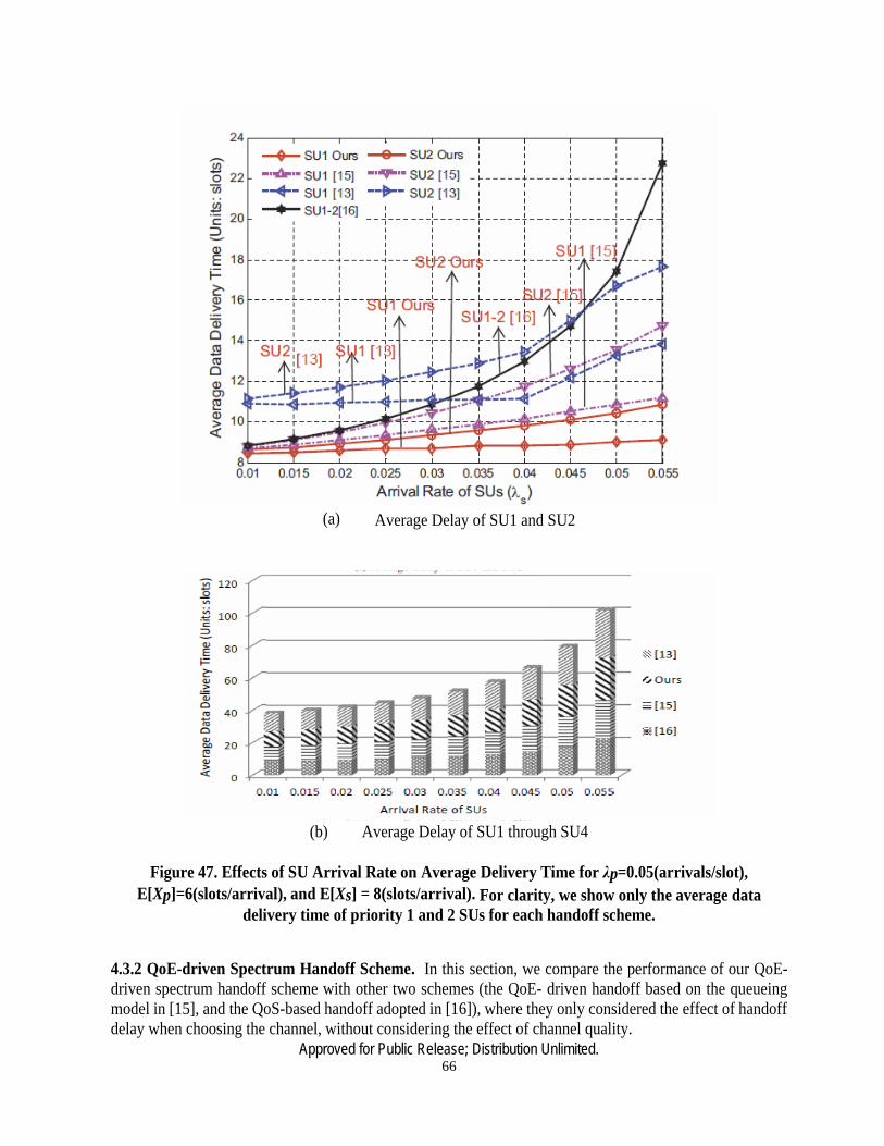
Approved for Public Release; Distribution Unlimited. 66
(a) Average Delay of SU1 and SU2
(b) Average Delay of SU1 through SU4
Figure 47. Effects of SU Arrival Rate on Average Delivery Time for λp=0.05(arrivals/slot),
E[Xp]=6(slots/arrival), and E[Xs] = 8(slots/arrival). For clarity, we show only the average data delivery time of priority 1 and 2 SUs for each handoff scheme.
4.3.2 QoE-driven Spectrum Handoff Scheme. In this section, we compare the performance of our QoE-driven spectrum handoff scheme with other two schemes (the QoE- driven handoff based on the queueing model in [15], and the QoS-based handoff adopted in [16]), where they only considered the effect of handoff delay when choosing the channel, without considering the effect of channel quality.

Approved for Public Release; Distribution Unlimited. 67
(a) Average Delay of SU1 and SU2
(b) Average Delay of SU1 through SU4
Figure 48. Effects of SU Service Time on Average Delivery Time for λp=0.05(arrivals/slot), E[Xp]=6(slots/arrival), and λs=0.03(arrivals/slot). For clarity, we show only the average data delivery time averaged across all users and those of priority 1 and 2 SUs for each handoff scheme.

Approved for Public Release; Distribution Unlimited. 68
The video sequences were encoded using H.264/AVC JM reference software [67] for a GOP length of 30 frames at 30 frames/sec. The FR (30 frames/sec) and SBR (200Kbps) are fixed. The number of channels is M = 3 and the number of priority classes is N = 4, where class j has higher priority than class j + 1. Table 9 shows our simulation parameters. As in [13], we assume that SUs may experience different channel conditions. Table 10 shows different PERs of each channel and the delay deadline of each SU. However, the total PER of the three channels is almost the same for all SUs. Here we use the same type of traffic for all SUs, but assign different priorities to them (with different delay deadlines). The same channel status can be used for different video sequences.
TABLE 9. Simulation Parameters . Note: NULL denotes that the application has loose delay constrains and packets do not expire
TABLE 10. Comparisons of Total Packet Error Rate for Different Normalized Loads of PU (ρp)
In Table X we observe that the QoE-driven spectrum handoff has a lower TPER than the delay-driven scheme. The results are expected, since the delay-driven scheme does not consider the effect of channel errors, whereas QoE-driven schemes consider both the transmission delay and channel errors when choosing the target channel. Further, the QoE-driven handoff based on our queueing model has lower TPER than QoE-driven handoff based on the queueing model in [15], especially for higher priority SUs under heavy traffic load. This is because the queueing model in [15] does not allow a higher priority SU to interrupt the lower priority SU. The increased waiting time for the higher priority SU may cause its packet to be dropped when
SU CH1 CH2 CH3 dj (sec) Applications SU1 16% 3% 11% 0.5 Video Conference SU2 2% 18% 10% 2 Live Stream SU3 17% 9% 4% 4 Video on Demand SU4 10% 16% 4% NULL File Download

Approved for Public Release; Distribution Unlimited. 69
its delay exceeds the deadline for the heavy traffic load. However, our hybrid queueing model allows the higher priority SU to preempt the service of lower priority SU if the discretion rule is satisfied. Thus, it improves the performance of higher priority SUs. This is why in Table X the TPER of SU3 is much higher than SU1 since it can interrupt the service of SU3. The interrupted SU3 has to wait in the queue until all other SUs with higher priority complete their services.
The corresponding PSNR result for the Foreman video sequence is shown in Figure 49. For conciseness, only the PSNR results of SU connections with priorities 1 and 2 are shown in the figure. The QoE-driven handoff based on our queueing model has obvious improvement in terms of video PSNR compared to QoE-driven handof [15] and the delay-driven handoff.
Figure 49. Average PSNR (in SU1 and SU2) of Foreman Video Sequence (bit rate: 200kps) vs. The Normalized Load of PU (ρp) for λs =0.05 (arrivals/slot), E[Xs] = 10 (slots/arrival), and E[Xp] = 20
(slots/arrival). The lossless PSNR of Foreman sequence is 36.81dB.
4.3.3 MAL-based Spectrum Handoff Scheme. In this section, we evaluate the performance of our MAL-based spectrum handoff scheme. We first evaluate the performance gain of using the single-teacher (i.e., general AL-based) handoff over the RL-based scheme. Then, we evaluate the effect of multiple teachers.
One 480p whale show video sequence (the bit rate is 1Mbps), is used in the experiments. This sequence was encoded using H.264/AVC JM reference software [67] for a GOP length of 30 frames at 30 frames/sec. The number of channels is M = 3, and the number of priority classes of SU connections is N = 4. The PER of a channel is picked randomly from 2% to 10%. The arrival rate and the service time of the SU/PU connections are set as λp = 0.05(arrivals/slot), E[Xp] = 6(slots/arrival), λs = 0.05(arrivals/slot), and E[Xs] = 8(slots/arrival). The discount rate (γ) of RL-based QoE-driven handoff scheme is set to 0.6. The temperature υ in the softmax policy is set to 0.3.
Figure 50 shows the results of the expected MOS for the AL- and RL-based handoff schemes. The AL-enhanced handoff outperforms RL-based handoff, especially in the early stage of the transmission.

Approved for Public Release; Distribution Unlimited. 70
Particularly, the AL-based handoff converges much faster than the RL-based one. For the time slot > 3 ∗ 104, performance of the RL-based scheme is almost the same as the AL-based one (both will converge to the stable status eventually). This is because the newly joined SU in this experiment is almost static, and thus does not experience significantly different channel conditions. Therefore, its performance does not fluctuate much with the time.
(a) Static Environment
(b) Dynamic Environment
Figure 50. Comparison of RL-based and Our MAL-based Spectrum Handoff Schemes
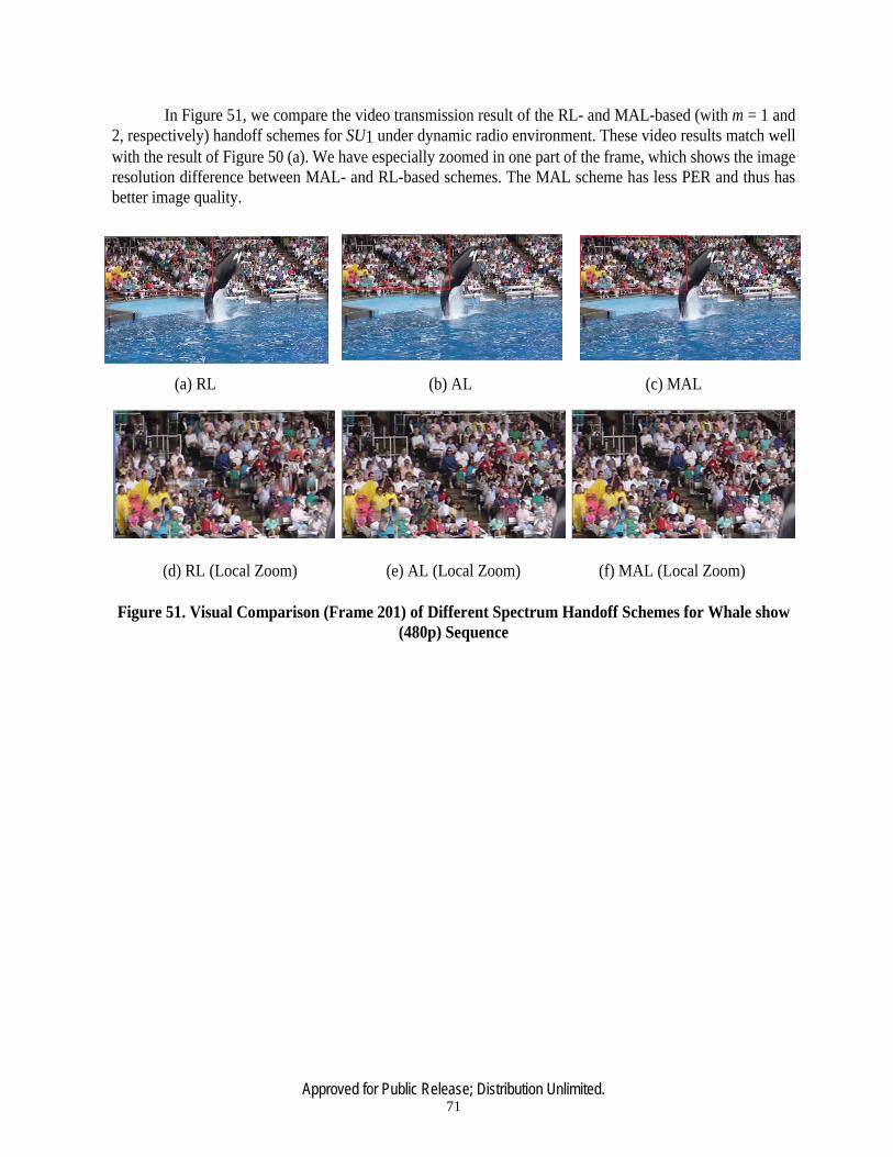
Approved for Public Release; Distribution Unlimited. 71
In Figure 51, we compare the video transmission result of the RL- and MAL-based (with m = 1 and 2, respectively) handoff schemes for SU1 under dynamic radio environment. These video results match well with the result of Figure 50 (a). We have especially zoomed in one part of the frame, which shows the image resolution difference between MAL- and RL-based schemes. The MAL scheme has less PER and thus has better image quality.
(a) RL (b) AL (c) MAL
(d) RL (Local Zoom) (e) AL (Local Zoom) (f) MAL (Local Zoom)
Figure 51. Visual Comparison (Frame 201) of Different Spectrum Handoff Schemes for Whale show (480p) Sequence

Approved for Public Release; Distribution Unlimited. 72
5.0 CONCLUSIONS In this project, we have designed a set of transfer-learning-based spectrum handoff schemes in CRNs. A comprehensive CRN testbed and many extensive simulations have also been built. We have described a CRN testbed with the following four components: (1) Spectrum sensing: We used compressive sensing algorithm to reduce the spectrum scanning time. The cyclostationary features are used to identify the spectrum characteristics due to their dominant patterns. (2) Spectrum mining: We then directly analyzed the compressive sensing samples without L1-norm signal reconstruction, based on machine learning algorithms. Our spectrum mining algorithms could classify the sensed free spectrum bands into different types. (3) Spectrum handoff : A TACT-based spectrum handoff decision scheme was designed to perform intelligent channel switching. It uses manifold learning to search an expert node, and transfers the knowledge from the expert node to a new node. (4) Rateless transmissions: we further used rateless codes to improve the CRN throughput. We used USRP nodes and GNU software to implement the above CRN platform. Such a testbed is comprehensive since it covers all essential CRN functions. Our testbed is suitable for further extensions without the need of rewriting the spectrum management functions. We have reported our iSM scheme based on machine learning methods. Our target was to achieve an intelligent spectrum handoff decision during rateless multimedia transmissions in dynamic CRN links. The handoff operation needs to have the good knowledge of channel quality so that it knows which channel to switch to. For accurate channel quality evaluation, we calculated the CUF that comprehensively measures the link quality. To adapt to the dynamic CRN channel conditions, we used CDF-enhanced Raptor codes to achieve intelligent link adaptation. A good link adaptation strategy can significantly reduce the occurrences of spectrum handoff. Our final goal is to make a correct iSM decision, which could be a spectrum handoff or wait-and-stay. The iSM decision is based on a teaching-and-learning based cognitive method, called TACT, to make optimal spectrum handoff among different SU states. The cognitive learning methods can achieve “cognitive” radio networks, not only in spectrum handoff tasks, but also for multimedia streaming over CRNs, dynamic routing establishment, etc. Finally, we have reported a hybrid PRP/NPRP M/G/1 queueing model with discretion rule to manage spectrum handoff for multimedia applications in CRNs. The queueing model is designed to meet the prioritized transmission requirements while avoiding the excessive delay caused by frequent spectrum handoffs. Based on the queueing model, MAL is integrated into the QoE-driven spectrum handoff scheme to allow a SU to learn from its neighbors, and performs spectrum handoff intelligently. Simulation results show that our approaches improve the end-user satisfaction in terms of delivery time and video PSNR.
Approved for Public Release; Distribution Unlimited. 73
REFERENCES
[1] Y.-C. Liang, K.-C. Chen, G. Y. Li, and P. Mahonen, “Cognitive radio networking and communications: An overview,” IEEE Transactions on Vehicular Technology, vol. 60, no. 7, pp. 3386–3407, 2011.
[2] Yasir Saleem, Farrukh Salim, and Mubashir Husain Rehmani, “Routing and channel selection from cognitive radio network's perspective.” Comput. Electr. Eng. 42, C (February 2015), pp. 117-134.
[3] M. Bertocco, G. Gamba, A. Sona, and S. Vitturi, “Experimental characterization of wireless sensor networks for industrial applications,” IEEE Transactions on Instrumentation and Measurement, vol. 57, no. 8, pp. 1537-1546, Aug 2008.
[4] L. Angrisani, M. Bertocco, D. Fortin, and A. Sona, “Experimental study of coexistence issues between ieee 802.11b and ieee 802.15.4 wireless networks,” IEEE Transactions on Instrumentation and Measurement, vol. 57, no. 8, pp. 1514–1523, Aug 2008.
[5] F. C. Commission et al., “Spectrum Policy Task Force Report, FCC 02-155,” 2002. Accessible from https://transition.fcc.gov/sptf/files/SEWGFinalReport_1.pdf.
[6] Y. Wu, F. Hu, S. Kumar, Y. Zhu, A. Talari, N. Rahnavard, and J. D. Matyjas, “A Learning-Based QoE-Driven Spectrum Handoff Scheme for Multimedia Transmissions over Cognitive Radio Networks,” IEEE Trans. On Selected Areas in Communications, vol. 32, no. 11, pp. 2134–2148, 2014.
[7] X. Xing, T. Jing, Y. Huo, H. Li, and X. Cheng, “Channel quality prediction based on Bayesian inference in cognitive radio networks,” in IEEE INFOCOM, 2013, pp. 1465–1473.
[8] P. A. Iannucci, J. Perry, H. Balakrishnan, and D. Shah, “No symbol left behind: a link-layer protocol for rateless codes,” in 18th ACM Annual Intl. Conf. on Mobile Computing and Networking, Mobicom’12, Istanbul, Turkey, Aug 22-26, 2012, pp. 17–28.
[9] Y. Wu, S. Kumar, F. Hu, Y. Zhu, and J. D. Matyjas, “Cross-layer Forward Error Correction Scheme Using Raptor and RCPC Codes for Prioritized Video Transmission over Wireless Channels,” IEEE Trans. on Circuits and Systems for Video Technology, vol. 24, no. 6, pp. 1047–1060, 2014.
[10] Y. Wu, F. Hu, S. Kumar, J. D. Matyjas, Q. Sun, and Y. Zhu, “Apprenticeship learning based spectrum decision in multi-channel wireless mesh networks with multi-beam antennas,” IEEE Trans. on Mobile Computing, Vol. 16, no. 2, pp. 314-325, Feb. 1 2017.
[11] L. Giupponi, A. Galindo-Serrano, P. Blasco, and M. Dohler, “Docitive networks: an emerging paradigm for Dynamic Spectrum Management [dynamic spectrum management],” IEEE Trans. on Wireless Communication, vol. 17, no. 4, pp. 47–54, 2010.
[12] R. Li, Z. Zhao, X. Chen, J. Palicot, and H. Zhang, “Tact: A transfer actor-critic learning framework for energy saving in cellular radio access networks,” IEEE Trans. on Wireless Communications, vol. 13, no. 4, pp. 2000–2011, 2014.
[13] H.-P. Shiang and M. van der Schaar, “Queuing-based dynamic channel selection for heterogeneous multimedia applications over cognitive radio networks,” IEEE Transactions on Multimedia, vol. 10, no. 5, pp. 896–909, 2008.
[14] L. Zhang, T. Song, M. Wu, J. Guo, D. Sun, and B. Gu, “Modeling for spectrum handoff based on secondary users with different priorities in cognitive radio networks,” in IEEE International Conference on Wireless Communications & Signal Processing (WCSP), 2012, pp. 1–6.
[15] Y. Wu, F. Hu, S. Kumar, Y. Zhu, A. Talari, N. Rahnavard, and J. D. Matyjas, “A learning-based qoe-driven spectrum handoff scheme for multimedia transmissions over cognitive radio networks,” IEEE
Approved for Public Release; Distribution Unlimited. 74
Journal on Selected Areas in Communications, vol. 32, no. 11, pp. 2134–2148, 2014. [16] L.-C. Wang, C.-W. Wang, and C.-J. Chang, “Modeling and analysis for spectrum handoffs in cognitive
radio networks,” IEEE Transactions on Mobile Computing, vol. 11, no. 9, pp. 1499–1513, 2012. [17] C.-W. Wang and L.-C. Wang, “Modeling and analysis for proactive decision spectrum handoff in
cognitive radio networks,” in 2009 IEEE International Conference on Communications (ICC), pp. 1–6. [18] S.-U. Yoon and E. Ekici, “Voluntary spectrum handoff: a novel approach to spectrum management in
CRNs,” in 2010 IEEE International Conference on Communications (ICC), pp. 1–5. [19] Y. Song and J. Xie, “Prospect: A proactive spectrum handoff framework for cognitive radio ad hoc
networks without common control channel,” IEEE Transactions on Mobile Computing, vol. 11, no. 7, pp. 1127–1139, 2012.
[20] Y. Wu, F. Hu, S. Kumar, J. D. Matyjas, Q. Sun, and Y. Zhu, “Apprenticeship learning based spectrum decision in multi-channel wireless mesh networks with multi-beam antennas,” vol. 16, no. 2, pp. 314-325, Feb. 1 2017.
[21] A. Araujo, J. Garcia-Palacios, J. Blesa, F. Tirado, E. Romero, A. Samartin, and O. Nieto-Taladriz, “Wireless measurement system for structural health monitoring with high time-synchronization accuracy,” IEEE Transactions on Instrumentation and Measurement, vol. 61, no. 3, pp. 801–810, March 2012.
[22] M. Hamid, N. Bjorsell, W. Van Moer, K. Barbe, and S. Slimane, “Blind spectrum sensing for cognitive radios using discriminant analysis: A novel approach,” IEEE Transactions on Instrumentation and Measurement, vol. 62, no. 11, pp. 2912–2921, Nov 2013.
[23] L. Gonzales-Fuentes, K. Barbe, W. Van Moer, and N. Bjorsell, “Cognitive radios: Discriminant analysis for automatic signal detection in measured power spectra,” IEEE Transactions on Instrumentation and Measurement, vol. 62, no. 12, pp. 3351–3360, Dec 2013.
[24] Z. Chen, N. Guo, and R. C. Qiu, “Building a cognitive radio network testbed,” in Proceedings of the IEEE Southeastcon, TN, 2011. Pp. 91-96.
[25] R. C. Qiu, Z. Chen, N. Guo, Y. Song, P. Zhang, H. Li, and L. Lai, “Towards a real-time cognitive radio network testbed: architecture, hardware platform, and application to smart grid,” in Proceedings of the fifth IEEE Workshop on Networking Technologies for Software-Defined Radio and White Space, 2010. Boston, MA, USA, 2010, pp. 1-6.
[26] T. R. Newman and T. Bose, “A cognitive radio network testbed for wireless communication and signal processing education,” in Digital Signal Processing Workshop and 5th IEEE Signal Processing Education Workshop, 2009. DSP/SPE 2009. IEEE 13th. Marco Island, FL. pp. 757–761.
[27] R. C. Qiu, C. Zhang, Z. Hu, and M. C. Wicks, “Towards a large-scale cognitive radio network testbed: Spectrum sensing, system architecture, and distributed sensing,” Journal of Communications, vol. 7, no. 7, pp. 552–566, 2012.
[28] P. Sutton, J. Lotze, H. Lahlou, S. Fahmy, K. Nolan, B. Ozgul, T. W. Rondeau, J. Noguera, L. E. Doyle et al., “Iris: an architecture for cognitive radio networking testbeds,” IEEE Communications Magazine, vol. 48, no. 9, pp. 114–122, 2010.
[29] E. Luther, J. Dinolfo, and S. Katti, “Software defined radio provides new opportunities for hands-on RF education,” Proceedings of the Canadian Engineering Education Association, 2012. CEEA12, Paper 100, Winnipeg, MB, June 17-20, 2012.
[30] V. Havary-Nassab, S. Hassan, and S. Valaee, “Compressive detection for wide-band spectrum sensing,” in 2010 IEEE International Conference on Acoustics Speech and Signal Processing (ICASSP). 2010, pp. 3094–3097.
[31] F. Zeng, C. Li, and Z. Tian, “Distributed compressive spectrum sensing in cooperative multihop

Approved for Public Release; Distribution Unlimited. 75
cognitive networks,” IEEE Journal of Selected Topics in Signal Processing, vol. 5, no. 1, pp. 37–48, 2011.
[32] Y. Zhang, “Spectrum handoff in cognitive radio networks: Opportunistic and negotiated situations,” in IEEE International Conference on Communications, 2009. ICC’09. 2009, pp. 1–6.
[33] L.-C. Wang and C.-W. Wang, “Spectrum handoff for cognitive radio networks: Reactive-sensing or proactive sensing?” in. IPCCC 2008. IEEE International Performance, Computing and Communications Conference. Pp. 343–348.
[34] K. Kim, I. Akbar, K. K. Bae, J.-S. Um, C. M. Spooner, J. H. Reed et al., “Cyclostationary approaches to signal detection and classification in cognitive radio,” in DySPAN 2007. 2nd IEEE international symposium on New frontiers in dynamic spectrum access networks, 2007, pp. 212–215.
[35] J. C. Platt, “Methods and apparatus for building a support vector machine classifier,” Dec. 4 2001, US Patent 6,327,581.
[36] L. R. Rabiner, “A tutorial on hidden markov models and selected applications in speech recognition,” Proceedings of the IEEE, vol. 77, no. 2, pp. 257–286, 1989.
[37] E. B. Fox, E. B. Sudderth, M. I. Jordan, and A. S. Willsky, “An hdp-hmm for systems with state persistence,” in Proceedings of the 25th international conference on Machine learning. ACM, 2008, pp. 312–319.
[38] X.-y. ZHI, Z.-q. HE, and W.-l. WU, “A Novel Cooperation Strategy Based on Rateless Coding in Cognitive Radio Network,” IJACT: International Journal of Advancements in Computing Technology, vol. 4, no. 8, pp. 333–347, 2012.
[39] J. Perry, H. Balakrishnan, and D. Shah, “Rateless Spinal Codes,” in 10th ACM Workshop on Hot Topics in Networks, 2011, p. 6.
[40] J. Perry, P. A. Iannucci, K. E. Fleming, H. Balakrishnan, and D. Shah, “Spinal Codes,” in ACM SIGCOMM Conf. Applications, Technologies, Architectures, and Protocols for Computer Communication, 2012, pp. 49–60.
[41] E. Blossom, “Gnu radio: tools for exploring the radio frequency spectrum,” Linux journal, vol. 2004, no. 122, pp. 4, 2004.
[42] X. Chen and C. Yuen, “Efficient resource allocation in a rateless-coded mu-mimo cognitive radio network with QoS provisioning and limited feedback,” IEEE Trans. on Vehicular Technology, vol. 62, no. 1, pp. 395-399, 2013.
[43] Y. Ren, P. Dmochowski, and P. Komisarczuk, “Analysis and Implementation of Reinforcement Learning on a GNU radio cognitive radio platform,” in 5th Intl. Conf. Cognitive Radio Oriented Wireless Networks and Communications, Cannes, France, 2010.
[44] B. F. Lo and I. F. Akyildiz, “Reinforcement Learning based Cooperative Sensing in Sognitive Radio Ad HocNetworks,” in 21st IEEE Intl. Symposium Personal Indoor and Mobile Radio Communications (PIMRC). 2010, pp. 2244–2249.
[45] N. Hosey, S. Bergin, I. Macaluso, and D. O’Donohue, “Q-Learning for Cognitive Radios,” in Proceedings of the China-Ireland Information and Communications Technology Conf. (CIICT 2009). ISBN 9780901519672. National University of Ireland Maynooth, 2009.
[46] Z. Chen and R. C. Qiu, “Q-learning based Bidding algorithm for Spectrum Auction in Cognitive Radio,” in IEEE Southeastcon, 2011, pp. 409–412.
[47] Y. Dai and J. Wu, “Sense in order: Channel Selection for Sensing in Cognitive Radio Networks,” in 8th IEEE Intl. Conf. Cognitive Radio Oriented Wireless Networks (CROWNCOM), 2013, pp. 74–79.
[48] L. Zappaterra, “QoS-driven Channel Selection for Heterogeneous Cognitive Radio Networks,” in ACM Conf. CoNEXT Student Workshop, 2012, pp. 7–8.
[49] F. Zhu, X.-D. Zhang, Y.-F. Hu, and D. Xie, “Nonstationary Hidden Markov Models for Multi-aspect

Approved for Public Release; Distribution Unlimited. 76
Discriminative Feature Extraction from Radar Targets,” IEEE Trans. on Signal Processing, vol. 55, no. 5, pp. 2203–2214, 2007.
[50] A. Shokrollahi, “Raptor Codes,” IEEE Trans. on Information Theory, vol. 52, no. 6, pp. 2551–2567, 2006.
[51] A. Gudipati and S. Katti, “Strider: Automatic Rate Adaptation and Collision Handling,” in ACM SIGCOMM Computer Communication Review, vol. 41, no. 4, 2011, pp. 158–169.
[52] R. G. Gallager, “Low-density Parity-check Codes,” IEEE Trans. on Information Theory, vol. 8, no. 1, pp. 21-28, 1962.
[53] U. Erez, M. D. Trott, and G. W. Wornell, “Rateless Coding for Gaussian Channels,” IEEE Trans. On Information Theory, vol. 58, no. 2, pp. 530–547, 2012.
[54] W. Tang, M. Z. Shakir, M. A. Imran, R. Tafazolli, and M.-S. Alouini, “Throughput Analysis for Cognitive Radio Networks with Multiple Primary Users and Imperfect Spectrum Sensing,” IET Communications, vol. 6, no. 17, pp. 2787–2795, 2012.
[55] A. D. Redish, S. Jensen, A. Johnson, and Z. Kurth-Nelson, “Reconciling Reinforcement Learning Models with Behavioral Extinction and Renewal: Implications for Addiction, Relapse, and Problem Gambling.” Psychological review, vol. 114, no. 3, p. 784, 2007.
[56] S. Zheng, X. Yang, S. Chen, and C. Lou, “Target channel sequence selection scheme for proactive-decision spectrum handoff,” IEEE Communications Letters, vol. 15, no. 12, pp. 1332–1334, 2011.
[57] Y. Zhang, “Spectrum handoff in cognitive radio networks: Opportunistic and negotiated situations,” in 2009 IEEE International Conference on Communications. IEEE, 2009, pp. 1–6.
[58] H.-P. Shiang and M. van der Schaar, “Online learning in autonomic multi-hop wireless networks for transmitting mission-critical applications,” IEEE Journal on Selected Areas in Communications, vol. 28, no. 5, pp. 728–741, 2010.
[59] J. Wang, H. Zhai, and Y. Fang, “Opportunistic packet scheduling and media access control for wireless lans and multi-hop ad hoc networks,” in Wireless Communications and Networking Conference, 2004. WCNC. 2004 IEEE, vol. 2. IEEE, 2004, pp. 1234–1239.
[60] R. W. Conway, W. L. Maxwell, and L. W. Miller, “Theory of scheduling. 1967,” Addison-Wesley, Reading, Mass, M. Eisenberg, Two queues with changeover times, Oper Res.(2), vol. 19, pp. 386–401, 1971.
[61] A. Lertsinsrubtavee, N. Malouch, and S. Fdida, “Controlling spectrum handoff with a delay requirement in cognitive radio networks,” in 2012 21st International Conference on Computer Communications and Networks (ICCCN). IEEE, 2012, pp. 1–8.
[62] A. Khan, L. Sun, E. Jammeh, and E. Ifeachor, “Quality of experience-driven adaptation scheme for video applications over wireless networks,” IET communications, vol. 4, no. 11, pp. 1337–1347, 2010.
[63] P. Abbeel and A. Y. Ng, “Apprenticeship learning via inverse reinforcement learning,” in Proceedings of the twenty-first international conference on Machine learning. ACM, 2004, pp. 1.
[64] A. Galindo-Serrano, L. Giupponi, P. Blasco, and M. Dohler, “Learning from experts in cognitive radio networks: the docitive paradigm,” in 2010 Proceedings of the Fifth International Conference on Cognitive Radio Oriented Wireless Networks and Communications. IEEE, 2010, pp. 1–6.
[65] A. Banerjee, S. Merugu, I. S. Dhillon, and J. Ghosh, “Clustering with bregman divergences,” Journal of machine learning research, vol. 6, no. Oct, pp. 1705–1749, 2005.
[66] “Wireless Regional Area Network (WRAN) Specific Requirements Part 22: Cognitive Wireless RAN Medium Access Control (MAC) and Physical Layer (PHY) Specifications: Policies and Procedures for Operation in the TV Bands,” IEEE Std. 802.22-2011, 2011.
[67] JVT, “H.264/avc reference software jm14.2, iso/iec std,” available from the following website: http://iphome.hhi.de/suehring/tml/download. Accessed in Oct 2015.

Approved for Public Release; Distribution Unlimited. 77
LIST OF SYMBOLS, ABBREVIATIONS, AND ACRONYMS
ACK Acknowledgement
AL Apprenticeship Learning
BER Bit Error Rate
BD Bregman Divergence
BPSK Binary Phase Shift Keying
CCMP Cyclostationary Compressive Measurement Processing
CDF Cumulative Distribution Function
CDP Cyclic Domain Profile
CHT Channel Holding Time
CI Channel Interference
CR Cognitive Radios
CRN Cognitive Radio Networks
CS Compressive Sensing
CSM Channel Selection Metric
CSMA Carrier Sense Multiple Access
CSP Compressive Signal Processing
CUF Channel Utilization Factor
DL Docitive Learning
FEC Forward Error Control
FFT Fast Fourier Transform
FPGA Field Programmable Gateway Access
FR Frame Rate
FT Fourier Transform
GOP Group of Pictures
HDP Hierarchical Dirichlet Process
HDSDR High Definition Software Defined Radio
HMM Hidden Markov Model
iSM Intelligent Spectrum Mobility
LT codes Luby Transfer Codes
MAC Medium Access Control
Approved for Public Release; Distribution Unlimited. 78
MAL Multi-Teacher Apprenticeship Learning
MDP Markov Decision Process
MIMO Multiple Input Multiple Output
ML Maximum Likelihood
MOS Mean Opinion Score
NPRP Nonpreemptive Priority
OFDM Orthogonal Frequency Division Multiple Access
PDR Packer Dropping Rate
PER Packet Error Rate
PRC Prioritized Raptor Codes
PSNR Peak SNR
PU Primary User
QoE Quality of Experience
QoS Quality of Service
QPSK Quadrature Phase Shift Keying
RCS Random Channel Selection
RL Reinforced Learning
Rx Reception
SCF Spectral Correlation Function
SNRs Signal-to-Noise Ratios
SU Secondary User
SVM Support Vector Machine
TACT Transfer Actor-Critic Learning
TD Time Difference
TDMA Time Division Multiple Access
TH Throughput
TPER Total Packet Error Rate
Tx Transmission
UDP User Datagram Packet
UEP Unequal Error Protection
USRP Universal Software Radio Peripheral