Intelligent Memory Management Heuristics

APPROVED: Paul Tarau, Major Professor Roy T. Jacob, Committee Member David Barrett, Committee Member Rada Mihalcea, Committee Member Robert Brazile, Program Coordinator Krishna Kavi, Chair of the Department of

Computer Science Sandra L. Terrell, Interim Dean of the Robert B.

Toulouse School of Graduate Studies

INTELLIGENT MEMORY MANAGEMENT HEURISTICS

Pradeep Panthulu, B.E

Thesis Prepared for the Degree of

MASTER OF SCIENCE

UNIVERSITY OF NORTH TEXAS

December 2003

Panthulu, Pradeep, Intelligent Memory Management Heuristics. Master of

Science (Computer Science), December 2003, 63 pp., 5 tables, 20 illustrations,

references, 16 titles.

Automatic memory management is crucial in implementation of runtime systems

even though it induces a significant computational overhead. In this thesis I explore the

use of statistical properties of the directed graph describing the set of live data to decide

between garbage collection and heap expansion in a memory management algorithm

combining the dynamic array represented heaps with a mark and sweep garbage collector

to enhance its performance.

The sampling method predicting the density and the distribution of useful data is

implemented as a partial marking algorithm. The algorithm randomly marks the nodes of

the directed graph representing the live data at different depths with a variable probability

factor p. Using the information gathered by the partial marking algorithm in the current

step and the knowledge gathered in the previous iterations, the proposed empirical

formula predicts with reasonable accuracy the density of live nodes on the heap, to decide

between garbage collection and heap expansion. The resulting heuristics are tested

empirically and shown to improve overall execution performance significantly in the

context of the Jinni Prolog compiler’s runtime system.

Copyright 2003

by

Pradeep Panthulu

ii

ACKNOWLEDGEMENTS

I would like to thank all my professors who have helped me in gaining in-depth

knowledge of the concepts of Computer Science. I am grateful to my major professor

Paul Tarau for guiding me through the course of my study. I would like to thank Nancy

Glenn of University of South Carolina, for introducing to me the possibility of the

application of statistical methods in my research. I also like to thank all of my committee

members David Barrett, Rada Mihalcea, Tom Jacob for their valuable suggestions and

support.

iii

TABLE OF CONTENTS

ACKNOWLEDGEMENTS............................................................................................... iii

LIST OF TABLES............................................................................................................. vi

LIST OF FIGURES .......................................................................................................... vii

INTRODUCTION .............................................................................................................. 1

1.1 MEMORY MANAGEMENT OVERVIEW ............................................................ 1

1.2 DIRECTED GRAPH MODELS FOR MEMORY MANAGEMENT ..................... 5

1.3 STATISTICAL PROPERTIES OF DIRECTED GRAPHS..................................... 8

PROBLEM DESCRIPTION............................................................................................. 10

2.1 DYNAMIC MEMEORY MANAGEMENT IN RUNTIME SYSTEMS............... 10

2.2 STATISTICAL DETECTION OF GARBAGE COLLECTION OPPORTUNITY

....................................................................................................................................... 12

EMPIRICAL EVALUATION.......................................................................................... 15

3.1 EXPERIMENT 1: ................................................................................................... 15

3.2 EXPERIMENT 2 .................................................................................................... 25

CONCLUSIONS AND FUTURE WORK....................................................................... 34

APPENDIX A................................................................................................................... 35

PSEUDO CODE OF THE ALGORITHM ....................................................................... 35

APPENDIX B................................................................................................................... 38

GC.PL ............................................................................................................................... 38

iv

APPENDIX C................................................................................................................... 40

BOYER.PL ....................................................................................................................... 40

APPENDIX D................................................................................................................... 50

TAK.PL............................................................................................................................. 50

APPENDIX E ................................................................................................................... 52

INPUT FILE TO PAJEK GENERATOR “INPUT.NET”................................................ 52

APPENDIX F ................................................................................................................... 59

MATLAB FORMULAE................................................................................................... 59

REFERENCE LIST: ......................................................................................................... 62

v

LIST OF TABLES

1.1 SAMPLES OF NODES GENERATED BY GC.PL………………………….……9

3.1 ANALYZED VALUES OF β - PARTIAL MARKING.…………………………..17

3.2 OUTPUT OF GC.PL – WITH PARTIAL MARKING……………………………17

3.3 ANALYZED VALUES OF β - WITH OUT REUSING PARTIAL MARKING…26

3.4 OUTPUT OF GC.PL – WITHOUT REUSING PARTIAL MARKING…………..26

vi

LIST OF FIGURES

Figure 1.1: Marking Phase of the GC ................................................................................. 4

Figure 1.2 Graph representation of live data on the heap ................................................... 8

Figure 3.1 Gc.pl Experiment 1; Depth Vs No. of Nodes.................................................. 18

Figure 3.2 Gc.pl Experiment 1; Projected to Total Nodes Vs No. of Nodes.................... 19

Figure 3.3 Gc.pl Result after applying the empirical formula .......................................... 20

Figure 3.4 Boyer.pl Experiment 1 Depth Vs No. of Nodes.............................................. 21

Figure 3.5 Boyer.pl Experiment 1 Projected to Total Nodes Vs Number of Nodes......... 22

Figure 3.6 Boyer.pl Result after applying the empirical formula ..................................... 22

Figure 3.7 Tak.pl Experiment 1 Depth Vs No. of Nodes ................................................. 23

Figure 3.8 Tak.pl Experiment 1 Projected to Total Nodes Vs No. of Nodes ................... 24

Figure 3.9 Tak.pl Result after applying the empirical formula......................................... 25

Figure 3.10 Gc.pl Experiment 2 Depth Vs No. of Nodes ................................................. 28

Figure 3.11 Gc.pl Experiment 2 Projected to Total Nodes Vs No. of Nodes................... 29

Figure 3.12 Gc.pl Result after applying the empirical formula ........................................ 29

Figure 3.13 Boyer.pl Experiment 2 Depth Vs No. of Nodes............................................ 30

Figure 3.14 Boyer.pl Experiment 2 Projected to Total Nodes Vs No. of Nodes.............. 31

Figure 3.15 Boyer.pl Result after applying the empirical formula ................................... 31

Figure 3.16 Tak.pl Experiment 2 Depth Vs No. of Nodes ............................................... 32

Figure 3.17 Tak.pl Experiment 2 Projected to Total Nodes Vs No. of Nodes ................. 33

Figure 3.18 Tak.pl Result after applying the empirical formula....................................... 33

vii

CHAPTER 1

INTRODUCTION

1.1 MEMORY MANAGEMENT OVERVIEW

Memory management is a field of computer science, which is vital for the

effective utilization of the computer resources. Memory management can be at various

levels between the user program and the memory hardware. Operating systems provide

an illusion of more main memory than what is actually present and create a virtual

memory, which makes it possible to run many programs simultaneously. Application

level memory management deals with the allocation and reclamation of the memory used

by a user program. It can be classified into manual memory management and automatic

memory management.

Manual memory management is in which programmer explicitly allocates and

reclaims the memory after its use. One of the examples for this type of memory

management is malloc and free operations in the C language. This type of memory

management technique has an advantage of knowing the exact inner workings of the

program. The main disadvantage of this technique is that it requires a lot of extra

programming to keep track of the liveness information of the objects or variables

allocated in the program. This causes a memory overhead and reduces the efficiency of

the program.

In automatic memory management, routines are provided by the programming

language to recycle the memory which is not reachable from the program variables.

1

These types of memory managers are also called as garbage collectors. Garbage

collectors overcome the memory overhead problem of the manual memory managers and

improve the efficiency of a program. One of the examples of this type of memory

management is implementation of garbage collectors in Java. Because of the advantages

of the automatic memory management, most of the modern runtime systems use different

variations of them to improve the performance.

Automatic memory managers can be classified as reference count collectors and

tracing collectors. A reference count collector keeps track of the references to a memory

block from other memory blocks. Different variations of the reference count collectors

like deferred reference collectors make garbage collection procedures efficient. In a

simple reference counting algorithm, reference count is maintained for each object, and

the count is increased when there is a new reference to the object and decremented if a

reference is lost or changed. If the count decreases to zero during the course of the

execution of the program, the object is considered to be unreachable and hence

reclaimed. One of the major disadvantages is that this technique fails to recycle memory

when there are loops between the objects.

Tracing collectors[3] follow the pointers from the program variables (also called

root sets), and mark all the reachable memory blocks and the unmarked memory used by

the user program as temporary variables is reclaimed. The different types of tracing

collectors that are frequently used are Copying collectors, Generational collectors,

Incremental counters and Mark and Sweep collectors.

2

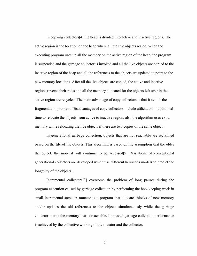
In copying collectors[4] the heap is divided into active and inactive regions. The

active region is the location on the heap where all the live objects reside. When the

executing program uses up all the memory on the active region of the heap, the program

is suspended and the garbage collector is invoked and all the live objects are copied to the

inactive region of the heap and all the references to the objects are updated to point to the

new memory locations. After all the live objects are copied, the active and inactive

regions reverse their roles and all the memory allocated for the objects left over in the

active region are recycled. The main advantage of copy collectors is that it avoids the

fragmentation problem. Disadvantages of copy collectors include utilization of additional

time to relocate the objects from active to inactive region; also the algorithm uses extra

memory while relocating the live objects if there are two copies of the same object.

In generational garbage collection, objects that are not reachable are reclaimed

based on the life of the objects. This algorithm is based on the assumption that the older

the object, the more it will continue to be accessed[9]. Variations of conventional

generational collectors are developed which use different heuristics models to predict the

longevity of the objects.

Incremental collectors[3] overcome the problem of long pauses during the

program execution caused by garbage collection by performing the bookkeeping work in

small incremental steps. A mutator is a program that allocates blocks of new memory

and/or updates the old references to the objects simultaneously while the garbage

collector marks the memory that is reachable. Improved garbage collection performance

is achieved by the collective working of the mutator and the collector.

3

Mark and Sweep algorithm traces out all the objects that are directly or indirectly

reachable from the given set of root nodes (local variable on the stack and static variables

that refer to the objects) of a program. This phase is called as mark phase. In the next

phase the algorithm scans through the heap and reclaims all the objects that are not

marked (not reachable). This phase is called as sweep phase.

5 10

2 6 11

3 7 12

Figure 1.1: Marking Phase of the GC

Different steps in the working of the mark and sweep algorithm are explained from the

figure 1.1.

Mark and Sweep algorithm proceeds in a recursive manner and marks all the

memory blocks that can be reached from the program variables. In the first step of the

marking phase, memory blocks 2, 3 and 4 are marked. In the second step, block 5 is

marked since it is reachable from block 2; similarly, blocks 7 and 8 are marked. In the

third step blocks 6 and 11 are marked since they are reachable from 5. In the next step

1 (Root set)

4 8 13

9 14

4

block 6 tries to mark block 2, which is already marked; hence nothing happens in this

step. When the mark phase terminates, all the blocks that are reachable from the root set

are marked, irrespective of loops between the memory blocks. In the sweep phase of the

algorithm, all the unmarked memory blocks (9, 10, 12, and 13) are recycled.

One of the drawbacks of this algorithm is that the mark phase has a complexity

proportional to that of the live data on the heap. If the heap has a sufficiently dense live

data distribution, this algorithm consumes a significant amount of computation power.

Moreover this algorithm should be executed without interruptions; otherwise the marked

nodes before interruption might not be valid and hence the algorithm should start the

whole process of marking from the root set.

In this study I will explore the statistical properties of the directed graphs which

describe the live data on the heap, to improve the performance of the traditional garbage

collectors.

1.2 DIRECTED GRAPH MODELS FOR MEMORY MANAGEMENT

Application of graphs to describe the physical properties in the real world has

yielded spectacular results. For example, as Kumar et al.[8] have shown that power law

degree distribution to describe the nodes in World Wide Web gives an insight into the

dynamic nature of the connectivity and thus helps in some applications to predict the

optimal route for the network packets in the internet. Random graphs are a special case of

graphs in which the graphs are built over probability space[5]. A random graph G(n,p)

where n is a positive integer and 0≤p≤1, is a probability space over the set of the graphs

on the set of vertex{1,…,n}, and is described by

5

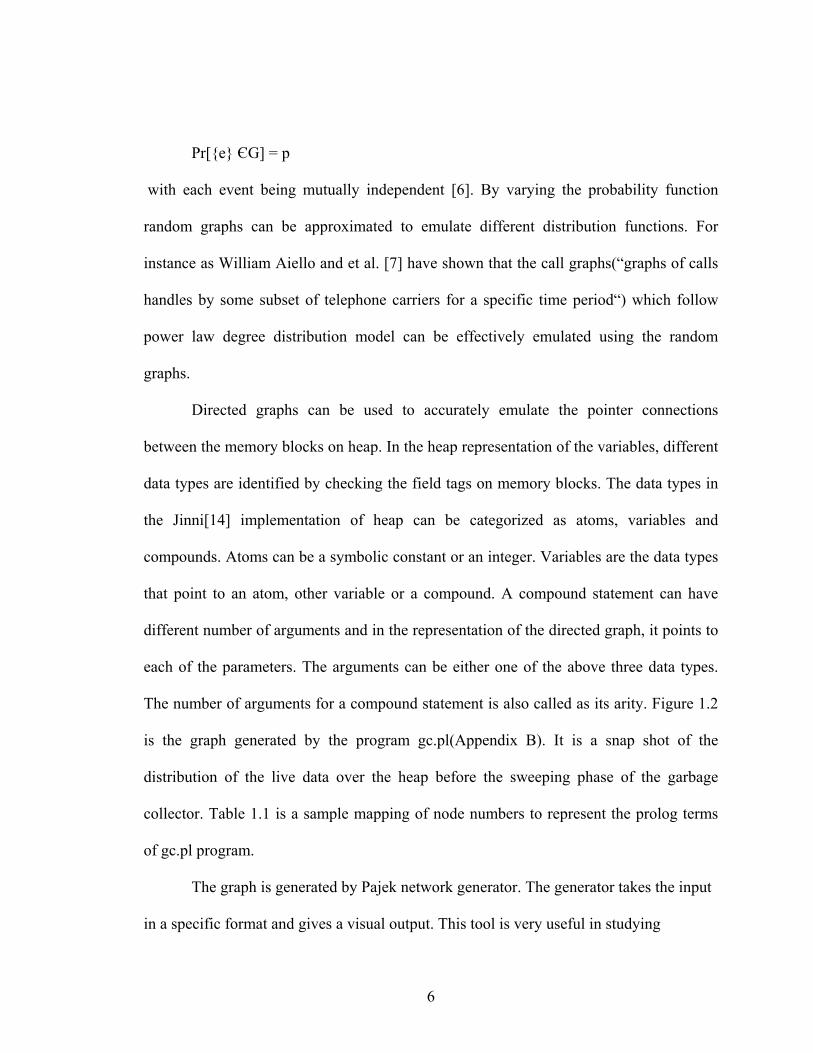
Pr[{e} ЄG] = p

with each event being mutually independent [6]. By varying the probability function

random graphs can be approximated to emulate different distribution functions. For

instance as William Aiello and et al. [7] have shown that the call graphs(“graphs of calls

handles by some subset of telephone carriers for a specific time period“) which follow

power law degree distribution model can be effectively emulated using the random

graphs.

Directed graphs can be used to accurately emulate the pointer connections

between the memory blocks on heap. In the heap representation of the variables, different

data types are identified by checking the field tags on memory blocks. The data types in

the Jinni[14] implementation of heap can be categorized as atoms, variables and

compounds. Atoms can be a symbolic constant or an integer. Variables are the data types

that point to an atom, other variable or a compound. A compound statement can have

different number of arguments and in the representation of the directed graph, it points to

each of the parameters. The arguments can be either one of the above three data types.

The number of arguments for a compound statement is also called as its arity. Figure 1.2

is the graph generated by the program gc.pl(Appendix B). It is a snap shot of the

distribution of the live data over the heap before the sweeping phase of the garbage

collector. Table 1.1 is a sample mapping of node numbers to represent the prolog terms

of gc.pl program.

The graph is generated by Pajek network generator. The generator takes the input

in a specific format and gives a visual output. This tool is very useful in studying

6

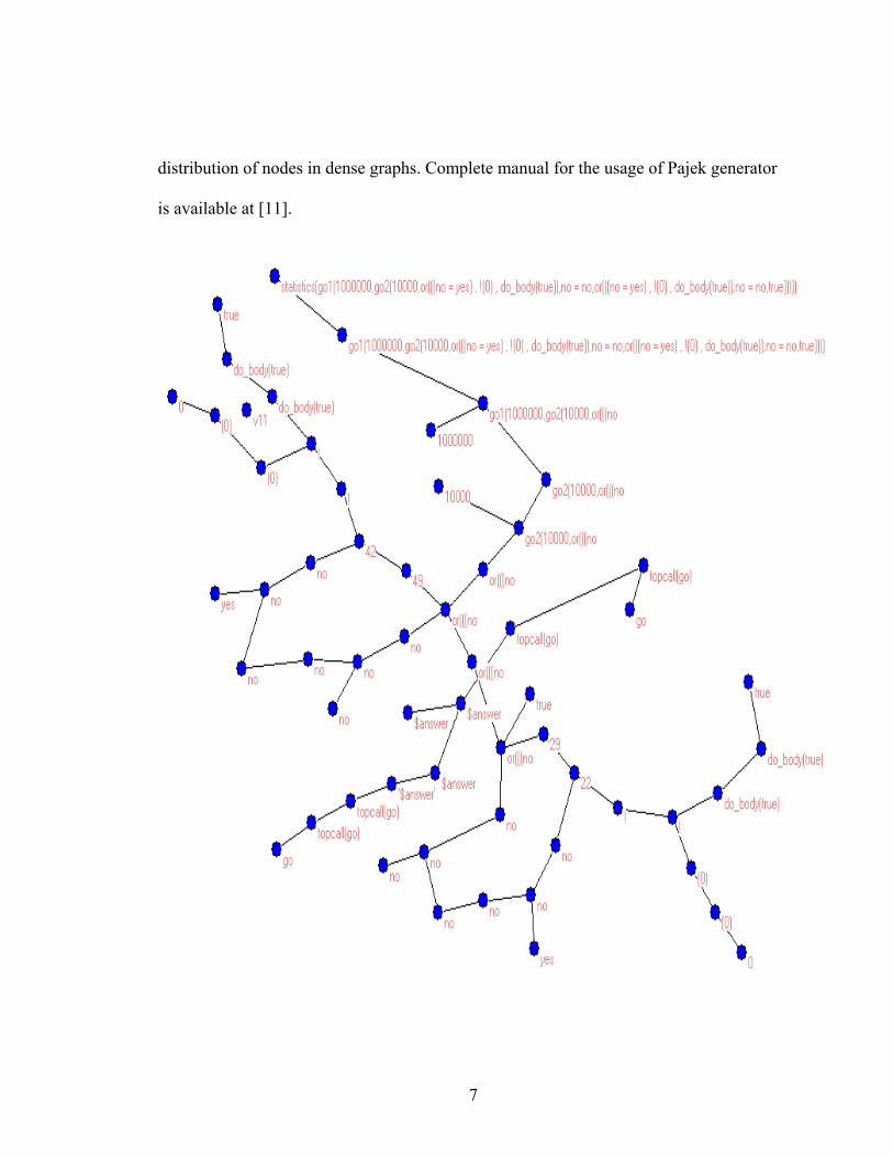
distribution of nodes in dense graphs. Complete manual for the usage of Pajek generator

is available at [11].

7

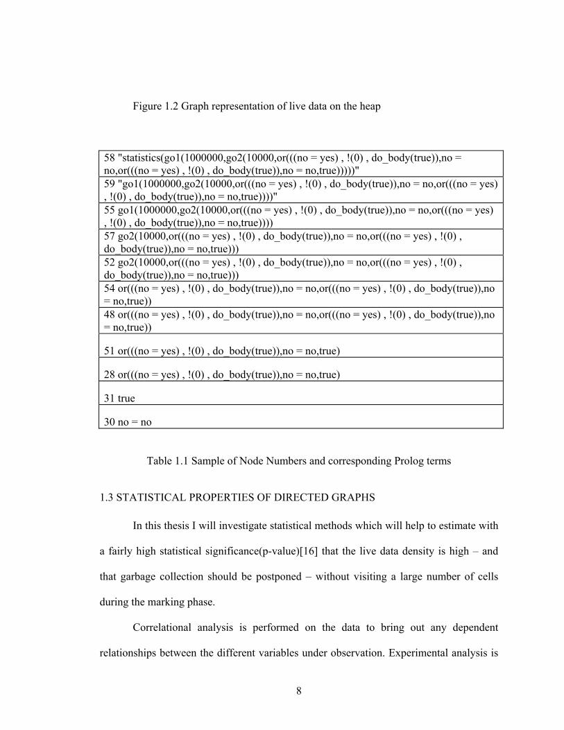
Figure 1.2 Graph representation of live data on the heap

58 "statistics(go1(1000000,go2(10000,or(((no = yes) , !(0) , do_body(true)),no = no,or(((no = yes) , !(0) , do_body(true)),no = no,true)))))" 59 "go1(1000000,go2(10000,or(((no = yes) , !(0) , do_body(true)),no = no,or(((no = yes) , !(0) , do_body(true)),no = no,true))))" 55 go1(1000000,go2(10000,or(((no = yes) , !(0) , do_body(true)),no = no,or(((no = yes) , !(0) , do_body(true)),no = no,true)))) 57 go2(10000,or(((no = yes) , !(0) , do_body(true)),no = no,or(((no = yes) , !(0) , do_body(true)),no = no,true))) 52 go2(10000,or(((no = yes) , !(0) , do_body(true)),no = no,or(((no = yes) , !(0) , do_body(true)),no = no,true))) 54 or(((no = yes) , !(0) , do_body(true)),no = no,or(((no = yes) , !(0) , do_body(true)),no = no,true)) 48 or(((no = yes) , !(0) , do_body(true)),no = no,or(((no = yes) , !(0) , do_body(true)),no = no,true))

51 or(((no = yes) , !(0) , do_body(true)),no = no,true)


31 true

30 no = no

Table 1.1 Sample of Node Numbers and corresponding Prolog terms

1.3 STATISTICAL PROPERTIES OF DIRECTED GRAPHS

In this thesis I will investigate statistical methods which will help to estimate with

a fairly high statistical significance(p-value)[16] that the live data density is high – and

that garbage collection should be postponed – without visiting a large number of cells

during the marking phase.

Correlational analysis is performed on the data to bring out any dependent

relationships between the different variables under observation. Experimental analysis is

8

done on the data by modifying a variable and checking how it influences the behavior of

the other variables in the data set. Experimental analysis can be effectively used to study

the causal relationship between variables.

Cluster analysis is used in the analysis of random graphs. It is used to establish a

classification system based on the output generated by the programs. The groups are

assigned accordingly to reflect the total number of nodes marked at a given step, given

the number of marked nodes at that step. This allocation will aid in the prediction of the

number of live nodes at a given step given the percentage of nodes sampled and the

number of marked nodes this percentage yields.

The underlying theory can be explained with the Central Limit Theorem[2],

which states that given a distribution with a meanµ and variance , the sampling

distribution of mean approaches a normal distribution with a mean

2σ

µ and variance

N2σ as the size of the sample N increases. It is observed that the data collected from the

programs with multiple runs for statistical analysis has a mean and has a definitive

standard deviation from the mean for each level of the directed graph.

9

CHAPTER 2

PROBLEM DESCRIPTION

Let DG be a directed graph describing the data on the heap, NDG be the set of

nodes in the graph DG, n be the cardinality of NDG and EDG be the set of edges of DG.

Given a subset R of NDG called the roots let CR be the connected component of DG

generated by following all the paths starting from R.

The memory reference inspired problem can be formulated as follows: determine

the probability that CR contains not more than k nodes of G, where k< n. Clearly, I would

like to solve this problem with a high probability yes/no answer –using a limited

sampling in G – with a computational effort that is significantly smaller than O(n). The

implementation of the heap and the partial marking algorithm is discussed in this chapter.

2.1 DYNAMIC MEMEORY MANAGEMENT IN RUNTIME SYSTEMS

On heap overflow (usually detected by catching an exception) the runtime system has

two choices – call the garbage collector or expand the heap as a part of memory

management algorithm. If the live data is sparse- garbage collection is a good idea,

despite of being a relatively costly process. If the live data is dense(and amount of

memory recovered is likely to be small) – doubling the heap size and avoiding the

garbage collection until the ratio of live data/ heap size becomes small enough, can

provide significant time savings.

10

For memory management techniques to be effective heap expansion and shrinking

operations should be efficient. Dynamic arrays are used in the implementation of heap in

Jinni runtime system[1], because they provide amortized O(1) complexity data structure.

If the heap overflow exception is caught, partial marking algorithm is invoked and based

on the predicted values, either heap expansion or garbage collection is done. If the

algorithm predicts that there is considerable amount of live data is on the heap, the heap

is doubled. Otherwise the heap is completely marked and the sweep phase in the garbage

collection algorithm recycles all the unmarked memory.

Jinni runtime system garbage collection procedures are a combination of mark

and sweep and copying collection algorithms. The program heap is divided into upper

heap and lower heap. Expansion or shrinking of the heap takes place with a factor of 2

i.e. the heap doubles if it runs out of memory or shrinks by half if it has more than 50% of

free space. After marking the heap and before the sliding phase is initiated, the algorithm

checks for viability of relocating the objects to the upper heap. The upper heap should

have enough space to accommodate the marked objects in the lower heap. If it fails, then

the heap is expanded, otherwise the algorithm copies each marked cell to the upper heap

and forward the links from old memory cells (vars and nonvars) to copied new cells but,

variables in new cells still point to old addresses. Before sliding the heap, all the memory

pointers are updated to point to the new locations of upper heap. All the choice points and

registers of the stack are relocated to the new memory cells.

After the updating the registers, the memory in the trial pointer cells is made to

point to an unbound variable at address 0. The heap slides from the upper heap to lower

11

heap and the relocation table in the lower heap is overwritten and the new reference value

of the heap top is updated. By implementing the mark and sweep algorithm with copying

and sliding, memory can be dynamically managed with arrays efficiently.

2.2 STATISTICAL DETECTION OF GARBAGE COLLECTION OPPORTUNITY

Memory graphs are generated starting from the root nodes (program variables)

and are extended as the nodes reference out to other memory locations. The marking

algorithm initiates the marking phase from the root set R. It randomly picks a node from

the root set and marks it. In the second step it looks for the references (edges in our

directed graph model) going out of the marked root set node. It picks an edge randomly

form the edge set , and will only proceed further if the probability factor generated

for the edge is less than the probability factor pi assigned at the beginning of the iteration.

Once it succeeds, the algorithm marks the edge as visited( ) and marks the node

referenced and the depth information is updated. This method of marking the heap is

repeated till all the edges are considered and the marking algorithm reaches the leaves of

the graph. The data for our statistical model is generated based on the results of the

marking algorithm. The parameters that are considered for this study are number of nodes

marked at each depth , the probability factor , the number of edges in the directed

graph , and total number of nodes on the heap . For each iteration the

probability factor is incremented by 0.1.

DGE

visitedE

dN ip

DGE TotalN

∑ += GarbagedTotal NNN

12

There are two variations of marking algorithm; one is in which the previously

marked information for lower probability factors is accounted. For example, if the

number of nodes marked for a probability factor 0.3 is 18, then for the probability factor

for 0.4(say) include all the nodes marked in the lower probability factor

iterations(0.1,0.2,0.3) and the new nodes added in the current iteration. In the second

variation of the algorithm, previously marked information is completely erased for each

iteration and the graph is traversed from the root set with varying probability factors.

One of the important parameters in the directed graph of memory graph is its

depth information. Depth of nodes in memory graphs is calculated by following the

references from the root set. Let d be the depth of the node k in a particular path traversal

of the graph, then is the depth of the node referenced by k. This process is repeated

till the leaves of the graph are reached. Depth information of nodes in the graphs is

recorded. This method of marking depth might lead to different depths for different path

traversals. In order to overcome the problem of different depth information for the same

node, all the depths calculated from different path traversals are stored in a vector. This

has an added advantage of finding the indegree[15] for each of the nodes, which is a

useful parameter for calculating the connectivity in the graph. If a node is encountered

with already marked depth, the second depth is assigned assuming that the node is a leaf,

so that no information is lost.

1+d

Having different depths to a node create another problem in further traversal from

the node, because node k might have depth of d1 and d2. To resolve this ambiguity the

node referenced by k is allocated a depth of { } 1,min 21 +dd .

13

The data is generated and tabulated for cluster analysis. The tabulated output of

the data generated by gc.pl is shown in the table. The partial marking algorithm’s pseudo

code is described in the appendix A. The data collected from the marking of heap is used

to evaluate the dependency of probability factor in the detection of the garbage collection

opportunity.

To establish the groups, I started by generating a random samples from a set of

programs with multiple runs. Gc.pl is used to establish the groups and the clusters are

analyzed by boyer.pl(Appendix C) and tak.pl(Appendix D) programs.

One of the obvious ways to decide about the opportunity for garbage collection –

is to stop the garbage collection algorithm after the marking phase, provided that the

majority of the cells have been marked. However, this has a paradoxical consequence that

the algorithm stops after the O(heapsize) cost has already been paid –assuming that most

cells are marked- a computational effort we would like to avoid in the first place!

Given the probabilistic nature of this estimation process, the partial marking

memory management algorithm will eventually perform the garbage collection

unconditionally after a number of failed estimates – but the mechanism for delaying it

works as an important computation time saving mechanism – as our empirical evaluation

will show.

14

CHAPTER 3

EMPIRICAL EVALUATION

The memory reference graph properties(nodes, depths and edges information) are

stored and trial runs are made with varying probability factor pi and the data is analyzed

by clustering. Let Nd be the number of nodes marked at depth d with the probability pi of

ph ( )ii pNG , where dN . the random gra iN

where Ntotallive is the total number of live nodes on the heap. Two sets of

experim

3.1 EXPERIMENT 1:

In this experiment, data is collected by partially marking the live nodes on the heap.

Starting from the probability factor of 0.1, th

2

1

22221

11211

n

n

XXX and can be represented in short by the set

∑=

=max

1d

totallivei NN ⊂

∑= itotallive NN

ents are performed to evaluate the distribution of the live data on the heap.

e memory graph is traversed and the edges

and nodes are marked at different depths of the directed graph. In the next traversal of the

heap, the probability factor is incremented by 0.1 and the total process is repeated

including the knowledge of the marking from previous iterations. In this experiment the

distribution of data in the triangular array format can be represented as follows

,.....,, XXX

...

,,........., ∑=d

dii xS

15

Variables are recorded at each depth of the process. The output of the collected nodes

is displayed in table 3.2. Based on the data generated by the programs and the clustering

analysis of the sets, I propose an empirical formula

βii pxy = where y is the predicted total live nodes on the heap

xi is the number of nodes marked at the step i

pi is the probability factor

β is the constant for each of the step i

to predict the total number of live nodes at each step. Based on the observation of the

distribution of the data and projecting it to the total number of nodes at each step i,

these values are calibrated. The variation of β is between -0.05 to +0.05

approximately depending on the program. Table 3.1 describes the different values of

β for different probability factors.

pi β

<=0.1 0.71

<=0.2 0.46

<=0.3 0.28

<=0.4 0.16

<=0.5 0.09

<=0.6 0.06

<=0.7 0.03

16

<=0.8 0.02

<=0.9 0.01

Table 3.1 Values of ‘β’ for EXPERIMENT 1

Depth 10% 20% 30% 40% 50% 60% 70% 80% 90% 100%0 0 1 1 4 4 4 4 4 4 41 0 3 4 9 9 9 9 9 9 92 1 7 8 13 13 13 13 13 13 133 2 9 11 17 17 17 17 17 17 174 2 9 12 19 19 19 19 19 19 195 2 9 13 20 21 21 21 21 21 216 2 10 14 21 22 22 22 22 22 227 3 13 17 24 25 25 25 25 25 258 4 16 20 27 28 28 28 28 28 289 5 18 25 33 34 34 35 35 35 35

10 6 19 28 36 39 39 40 40 40 4011 8 22 32 42 46 47 48 48 48 4812 9 24 36 47 51 52 53 53 53 5313 9 26 41 53 57 58 59 59 59 5914 9 28 43 55 59 60 61 61 61 6115 9 29 44 56 61 62 63 63 63 63

TOTAL MARKED=60/60 65538 Number of edges: 59 Max depth: 15 GC: words collected=65478, free=65476 gc time=312ms, total GC=726, trail=0, choice=0Java Memory: total=17580032 free=3744280

Table 3.2 Output Data from gc.pl with partial marking

17

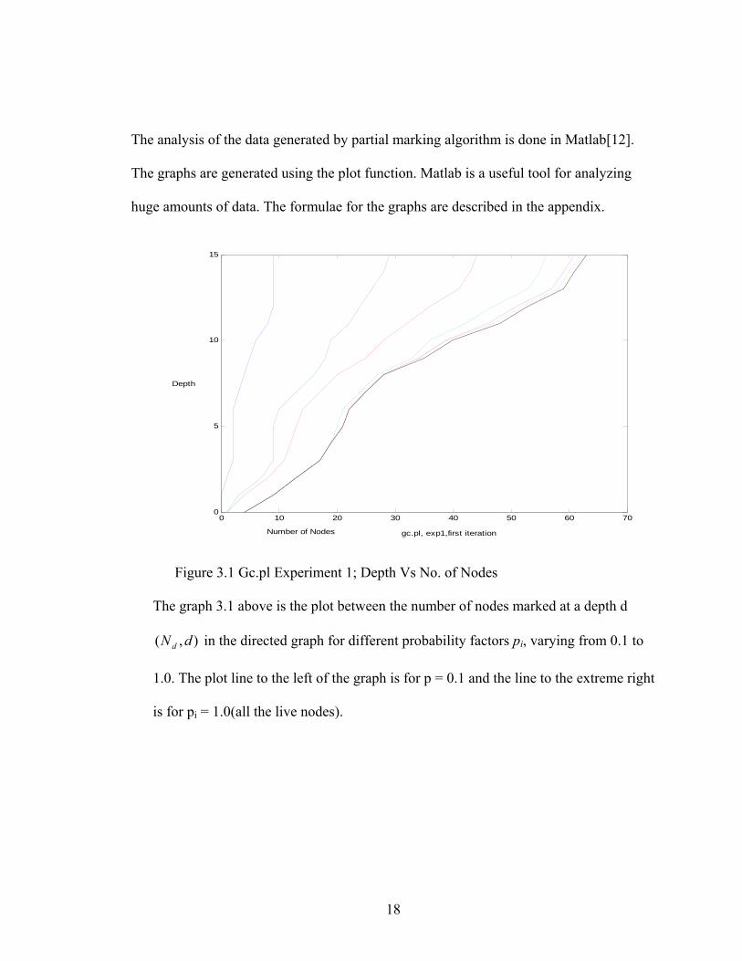
The analysis of the data generated by partial marking algorithm is done in Matlab[12].

The graphs are generated using the plot function. Matlab is a useful tool for analyzing

huge amounts of data. The formulae for the graphs are described in the appendix.

0 10 20 30 40 50 60 700

5

10

15

Number of Nodes

Depth

gc.pl, exp1,first iteration

Figure 3.1 Gc.pl Experiment 1; Depth Vs No. of Nodes

The graph 3.1 above is the plot between the number of nodes marked at a depth d

in the directed graph for different probability factors pi, varying from 0.1 to

1.0. The plot line to the left of the graph is for p = 0.1 and the line to the extreme right

is for pi = 1.0(all the live nodes).

),( dNd

18

0 10 20 30 40 50 60 700

10

20

30

40

50

60

70

Number of Nodes

Projectedto total Nodes

(gc.pl, x vs y ,exp1)

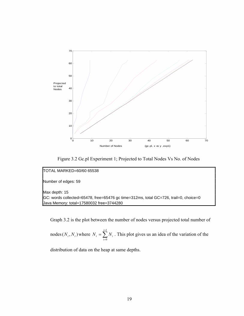
Figure 3.2 Gc.pl Experiment 1; Projected to Total Nodes Vs No. of Nodes

TOTAL MARKED=60/60 65538 Number of edges: 59 Max depth: 15 GC: words collected=65478, free=65476 gc time=312ms, total GC=726, trail=0, choice=0 Java Memory: total=17580032 free=3744280

Graph 3.2 is the plot between the number of nodes versus projected total number of

nodes where . This plot gives us an idea of the variation of the

distribution of data on the heap at same depths.

),( ti NN ∑=

=

=1

0

i

iit NN

19

0 10 20 30 40 50 60 700

10

20

30

40

50

60

70

Result after applying the empirical formula

Number of Nodes Gc.pl Exp1 First Iteration

Projectedto Total Nodes

p =0.1

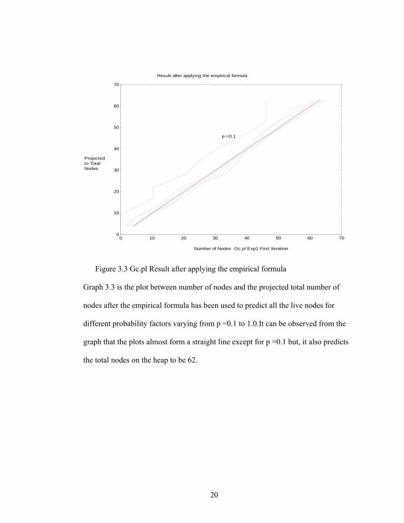
Figure 3.3 Gc.pl Result after applying the empirical formula

Graph 3.3 is the plot between number of nodes and the projected total number of

nodes after the empirical formula has been used to predict all the live nodes for

different probability factors varying from p =0.1 to 1.0.It can be observed from the

graph that the plots almost form a straight line except for p =0.1 but, it also predicts

the total nodes on the heap to be 62.

20

0 500 1000 1500 2000 2500 3000 35000

20

40

60

80

100

120

Number of Nodes

Depth

(boyer.pl, Exp1, First Iteration)

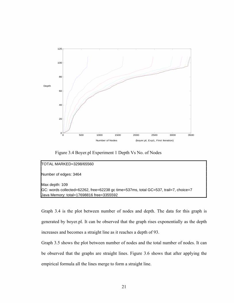
Figure 3.4 Boyer.pl Experiment 1 Depth Vs No. of Nodes

TOTAL MARKED=3298/65560 Number of edges: 3464 Max depth: 109 GC: words collected=62262, free=62238 gc time=537ms, total GC=537, trail=7, choice=7 Java Memory: total=17698816 free=3355592

Graph 3.4 is the plot between number of nodes and depth. The data for this graph is

generated by boyer.pl. It can be observed that the graph rises exponentially as the depth

increases and becomes a straight line as it reaches a depth of 93.

Graph 3.5 shows the plot between number of nodes and the total number of nodes. It can

be observed that the graphs are straight lines. Figure 3.6 shows that after applying the

empirical formula all the lines merge to form a straight line.

21

0 500 1000 1500 2000 2500 3000 35000

500

1000

1500

2000

2500

3000

3500

Number of Nodes


(boyer.pl, Exp1, First Iteration)

Figure 3.5 Boyer.pl Experiment 1 Projected to Total Nodes Vs Number of Nodes

0 500 1000 1500 2000 2500 3000 3500 40000

500

1000

1500

2000

2500

3000

3500Result after applying the empirical formula

Number of Nodes Boyer.pl, Exp1, First Iteration

Projected to Total Nodes

Figure 3.6 Boyer.pl Result after applying the empirical formula

22

0 50 100 150 200 250 300 350 400 450 5000

20

40

60

80

100

120

Number of Nodes (tak.pl, Exp1, First Iteration)

Depth

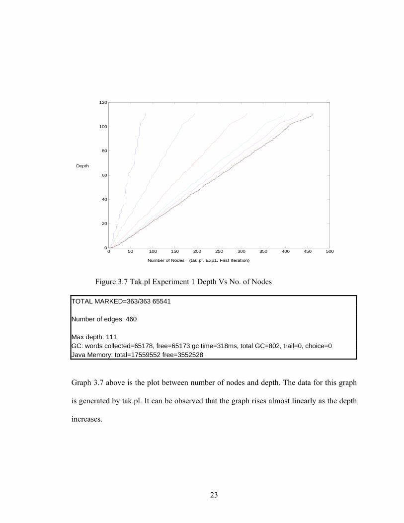
Figure 3.7 Tak.pl Experiment 1 Depth Vs No. of Nodes


Graph 3.7 above is the plot between number of nodes and depth. The data for this graph

is generated by tak.pl. It can be observed that the graph rises almost linearly as the depth

increases.

23

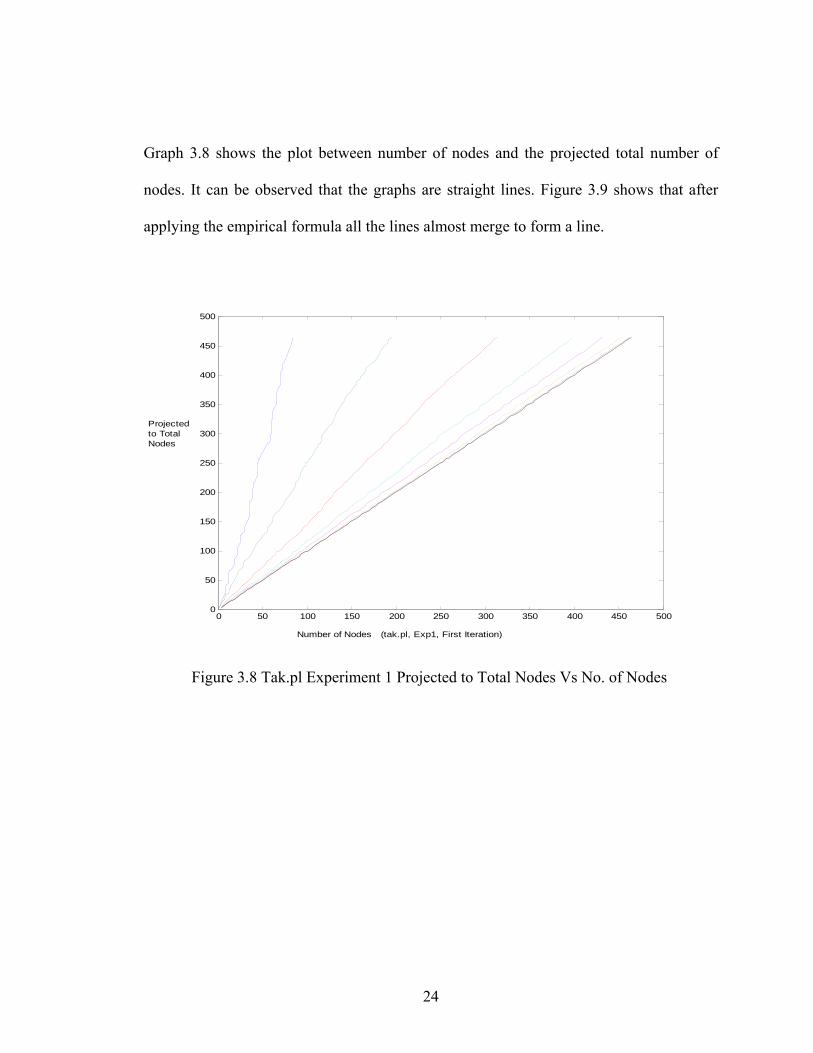
Graph 3.8 shows the plot between number of nodes and the projected total number of

nodes. It can be observed that the graphs are straight lines. Figure 3.9 shows that after

applying the empirical formula all the lines almost merge to form a line.

0 50 100 150 200 250 300 350 400 450 5000

50

100

150

200

250

300

350

400

450

500

Number of Nodes (tak.pl, Exp1, First Iteration)


Figure 3.8 Tak.pl Experiment 1 Projected to Total Nodes Vs No. of Nodes

24

0 50 100 150 200 250 300 350 400 450 5000

50

100

150

200

250

300

350

400

450

500


Number of Nodes Tak.pl Exp1 First Iteration


p =0.2

Figure 3.9 Tak.pl Result after applying the empirical formula

After analyzing all the graphs from three different programs it is observed that

distribution of nodes at different depths varies exponentially with the probability factor if

the number of nodes is significantly high as in boyer.pl (3464). The data for the graph is

chosen from a random run, out of multiple runs of the algorithm.

3.2 EXPERIMENT 2

In this experiment information is stored based on the number of nodes marked at each

of the probability factors not using the previously marked information of the nodes. In

each iteration, nodes are marked with increasing probability factor with out accounting

for the previous iterations. From the data gathered it can be observed that the constant β

converges to 0.5. The graphs in the subsequent sections are generated by different

25

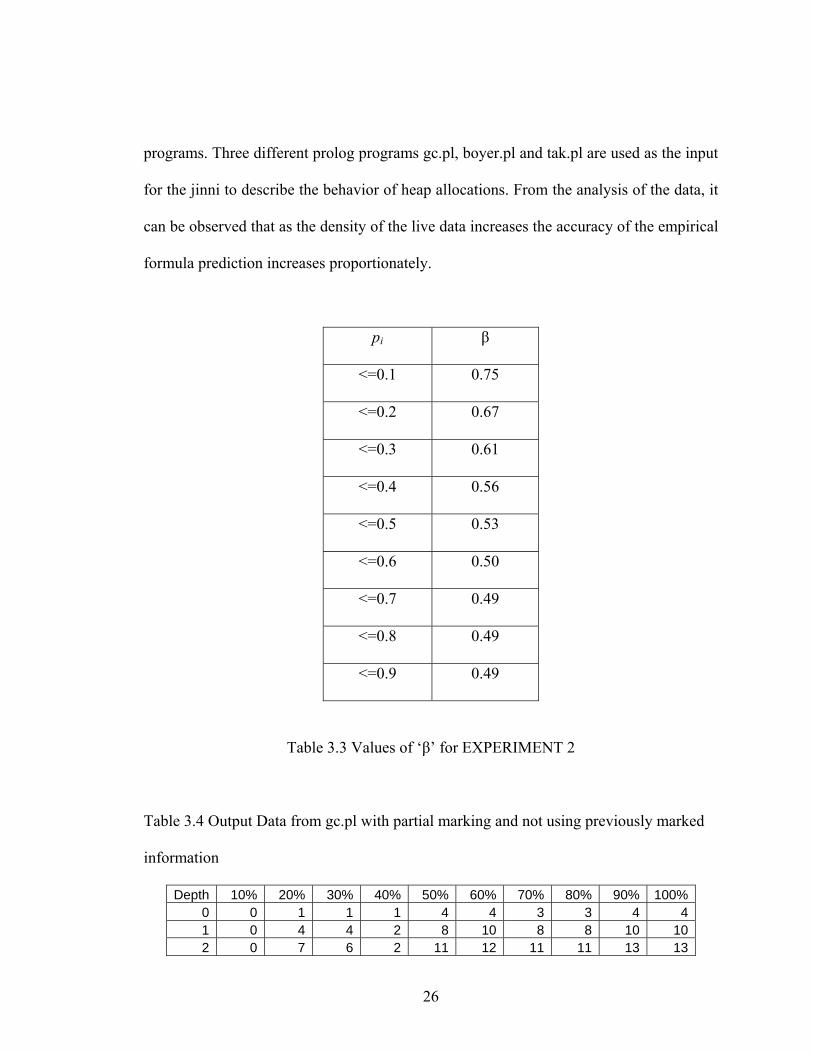
programs. Three different prolog programs gc.pl, boyer.pl and tak.pl are used as the input

for the jinni to describe the behavior of heap allocations. From the analysis of the data, it

can be observed that as the density of the live data increases the accuracy of the empirical

formula prediction increases proportionately.

pi β

<=0.1 0.75

<=0.2 0.67

<=0.3 0.61

<=0.4 0.56

<=0.5 0.53

<=0.6 0.50

<=0.7 0.49

<=0.8 0.49

<=0.9 0.49

Table 3.3 Values of ‘β’ for EXPERIMENT 2

Table 3.4 Output Data from gc.pl with partial marking and not using previously marked

information

Depth 10% 20% 30% 40% 50% 60% 70% 80% 90% 100%0 0 1 1 1 4 4 3 3 4 41 0 4 4 2 8 10 8 8 10 102 0 7 6 2 11 12 11 11 13 13

26

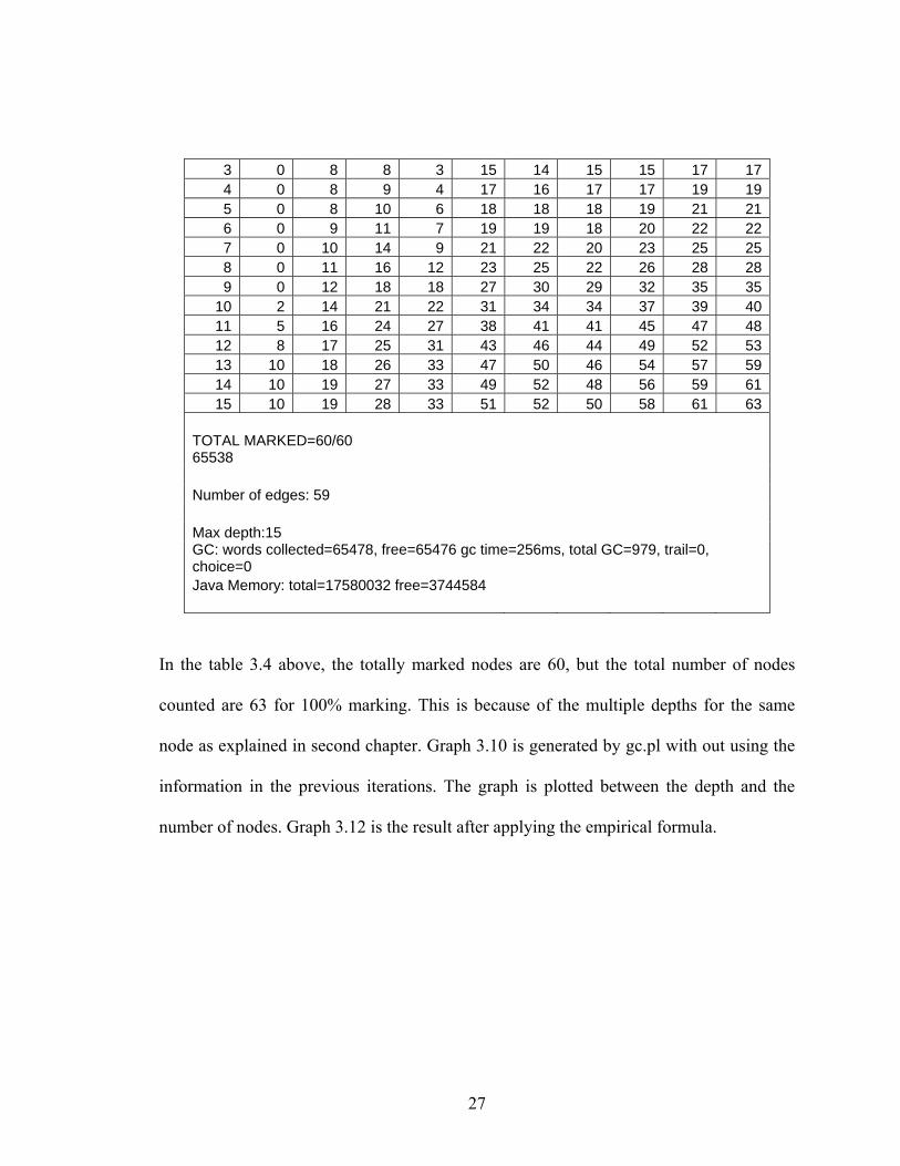
3 0 8 8 3 15 14 15 15 17 174 0 8 9 4 17 16 17 17 19 195 0 8 10 6 18 18 18 19 21 216 0 9 11 7 19 19 18 20 22 227 0 10 14 9 21 22 20 23 25 258 0 11 16 12 23 25 22 26 28 289 0 12 18 18 27 30 29 32 35 35

10 2 14 21 22 31 34 34 37 39 4011 5 16 24 27 38 41 41 45 47 4812 8 17 25 31 43 46 44 49 52 5313 10 18 26 33 47 50 46 54 57 5914 10 19 27 33 49 52 48 56 59 6115 10 19 28 33 51 52 50 58 61 63

TOTAL MARKED=60/60 65538 Number of edges: 59 Max depth:15 GC: words collected=65478, free=65476 gc time=256ms, total GC=979, trail=0, choice=0 Java Memory: total=17580032 free=3744584

In the table 3.4 above, the totally marked nodes are 60, but the total number of nodes

counted are 63 for 100% marking. This is because of the multiple depths for the same

node as explained in second chapter. Graph 3.10 is generated by gc.pl with out using the

information in the previous iterations. The graph is plotted between the depth and the

number of nodes. Graph 3.12 is the result after applying the empirical formula.

27

0 10 20 30 40 50 60 700

5

10

15

Number of Nodes (gc.pl, Exp2, Last Iteration)

Depth

Figure 3.10 Gc.pl Experiment 2 Depth Vs No. of Nodes

TOTAL MARKED=60/60 65538 Number of edges: 59 Max depth: 15 GC: words collected=65478, free=65476 gc time=313ms, total GC=2608, trail=0, choice=0Java Memory: total=17829888 free=3994584 runtime = [5118,4644] global_stack = [10843,54692] local_stack = [4,0] trail = [3,1] code = [20904,11864] symbols = [1020,0] htable = [2157,6035]

28

0 10 20 30 40 50 60 700

10

20

30

40

50

60

70

Number of Nodes (gc.pl, Exp2, Last Iteration)


Figure 3.11 Gc.pl Experiment 2 Projected to Total Nodes Vs No. of Nodes

0 20 40 60 80 100 1200

10

20

30

40

50

60

70


Number of Nodes Gc.pl Exp2 Last Iteration


p =0.1

Figure 3.12 Gc.pl Result after applying the empirical formula

29

0 2000 4000 6000 8000 10000 12000 14000 16000 180000

50

100

150

Number of Nodes (boyer.pl, Exp2, Last Iteration)

Depth

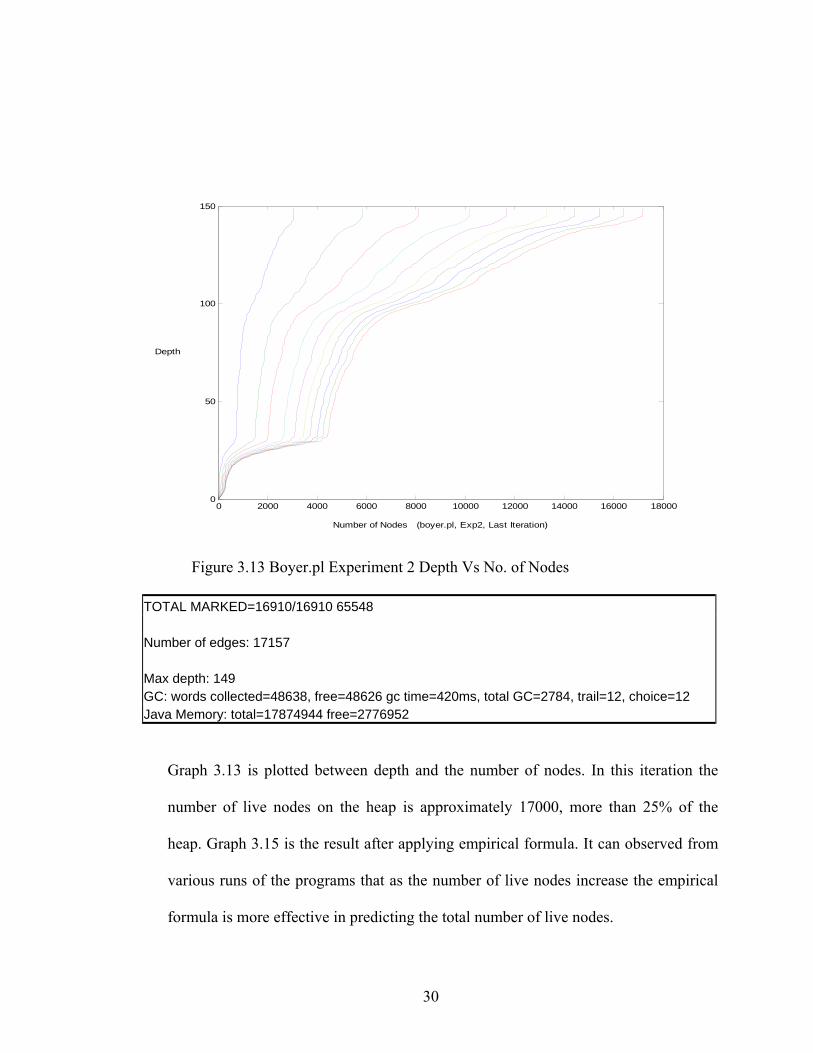
Figure 3.13 Boyer.pl Experiment 2 Depth Vs No. of Nodes


Graph 3.13 is plotted between depth and the number of nodes. In this iteration the

number of live nodes on the heap is approximately 17000, more than 25% of the

heap. Graph 3.15 is the result after applying empirical formula. It can observed from

various runs of the programs that as the number of live nodes increase the empirical

formula is more effective in predicting the total number of live nodes.

30

0 2000 4000 6000 8000 10000 12000 14000 16000 180000

2000

4000

6000

8000

10000

12000

14000

16000

18000

Number of Nodes (boyer.pl, Exp2, Last Iteration)


Figure 3.14 Boyer.pl Experiment 2 Projected to Total Nodes Vs No. of Nodes

0 2000 4000 6000 8000 10000 12000 14000 16000 180000

2000

4000

6000

8000

10000

12000

14000

16000

18000


Number of Nodes Boyer.pl Exp2 Last Iteration


Figure 3.15 Boyer.pl Result after applying the empirical formula

31

0 100 200 300 400 500 6000

20

40

60

80

100

120

140

Number of Nodes (tak.pl, Exp2, Last Iteration)

Depth

Figure 3.16 Tak.pl Experiment 2 Depth Vs No. of Nodes


Graphs 3.16, 3.17 and 3.18 are generated by the runs of tak.pl. The empirical formula

predictions are with in 10% error.

32

0 100 200 300 400 500 6000

100

200

300

400

500

600

Number of Nodes (tak.pl, Exp2, Last Iteration)

Projected to Total Nodes

Figure 3.17 Tak.pl Experiment 2 Projected to Total Nodes Vs No. of Nodes

0 100 200 300 400 500 6000

100

200

300

400

500

600


Number of Nodes Tak.pl Exp2 Last Iteration


Figure 3.18 Tak.pl Result after applying the empirical formula

33

CHAPTER 4

CONCLUSIONS AND FUTURE WORK

Statistical techniques when combined with the proposed partial marking

algorithm can be used to predict the actual size of the set of live nodes with a reasonable

accuracy. Considerable performance gain is achieved by using the predicting formula for

different programs. It is observed that the error ranges are from -0.05 to +0.05.

The scope of the future work would include studying of the degree distribution of

the nodes in the directed graph and also investigating different properties like

connectivity of the heap, existence of the giant component in a sufficiently large memory

graphs. Also, interpreting the importance of β approaching 0.5 in experiment 2 as the

probability factor reaches 1.0. Monte Carlo method [10] of approximation can be used for

effective prediction of the answer to the go/no go question with a fixed error rate. Related

work in the study of the connectivity between the heap objects is done by Martin Hirzel

et al. [9]

34

APPENDIX A

PSEUDO CODE OF THE ALGORITHM

35

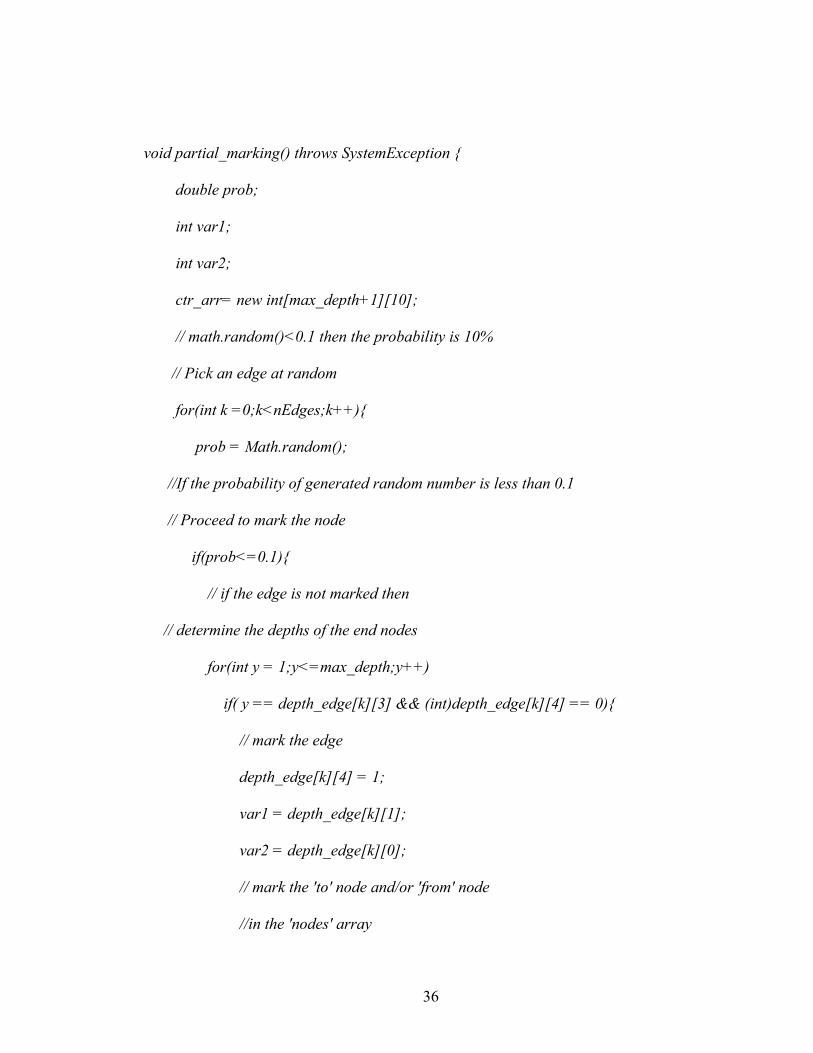
void partial_marking() throws SystemException {

double prob;

int var1;

int var2;

ctr_arr= new int[max_depth+1][10];

// math.random()<0.1 then the probability is 10%

// Pick an edge at random

for(int k =0;k<nEdges;k++){

prob = Math.random();

//If the probability of generated random number is less than 0.1

// Proceed to mark the node

if(prob<=0.1){

// if the edge is not marked then

// determine the depths of the end nodes

for(int y = 1;y<=max_depth;y++)

if( y == depth_edge[k][3] && (int)depth_edge[k][4] == 0){

// mark the edge

depth_edge[k][4] = 1;

var1 = depth_edge[k][1];

var2 = depth_edge[k][0];

// mark the 'to' node and/or 'from' node

//in the 'nodes' array

36

// increment the ctr_arr if 'to'

//and/or 'from' are unmarked

// check if 'to' node is marked

if(((int)nodes[var1][1]) == 0 ){

//If the ‘to’ node is not marked already

// Increment the counter at the respective depth of the node

++ctr_arr[y][0];

++nodes[var1][2];

// If the node has multiple depths

if(nodes[var1][2] == Depth[var1].size())

//mark the ’to’ node only after all the depths are exhausted

nodes[var1][1] = 1;

}

// check if 'from' node is marked

if(nodes[var2][1] == 0){

// If not marked increment the counter array at the depth of the node

++nodes[var2][2];

++ctr_arr[y-1][0];

// check if the node has multiple depths

if(nodes[var2][2] == Depth[var2].size())

nodes[var2][1] = 1;

37

APPENDIX B

GC.PL

38

% Benchmark gc

go:-go(100000),go1(1000000),go2(100).

go(N):-loop(N),statistics.

loop(0).

loop(N):-N>0,N1 is N-1,make_garbage(N1,_),loop(N1).

make_garbage(X,g(X)).

go1(N):-loop1(N,dummy),statistics.

loop1(0,_).

loop1(N,X):-N>0,N1 is N-1,make_garbage(X,X1),loop1(N1,X1).

go2(N) :-

mkfreelist(N,L), ctime(A), (mmc(N,L), fail ; true), ctime(B),

X is B - A, write(time(X)), nl, fail;

statistics.

mmc(N,L) :- N > 0,M is N - 1, mmc(M,L), !.

mmc(_,L) :- mkground(L).mkfreelist(N,L) :-

(N = 0 -> L = [] ;NN is N - 1, L = [_|R], mkfreelist(NN,R) ).

mkground([]).mkground([a|R]) :- mkground(R).

39

APPENDIX C

BOYER.PL

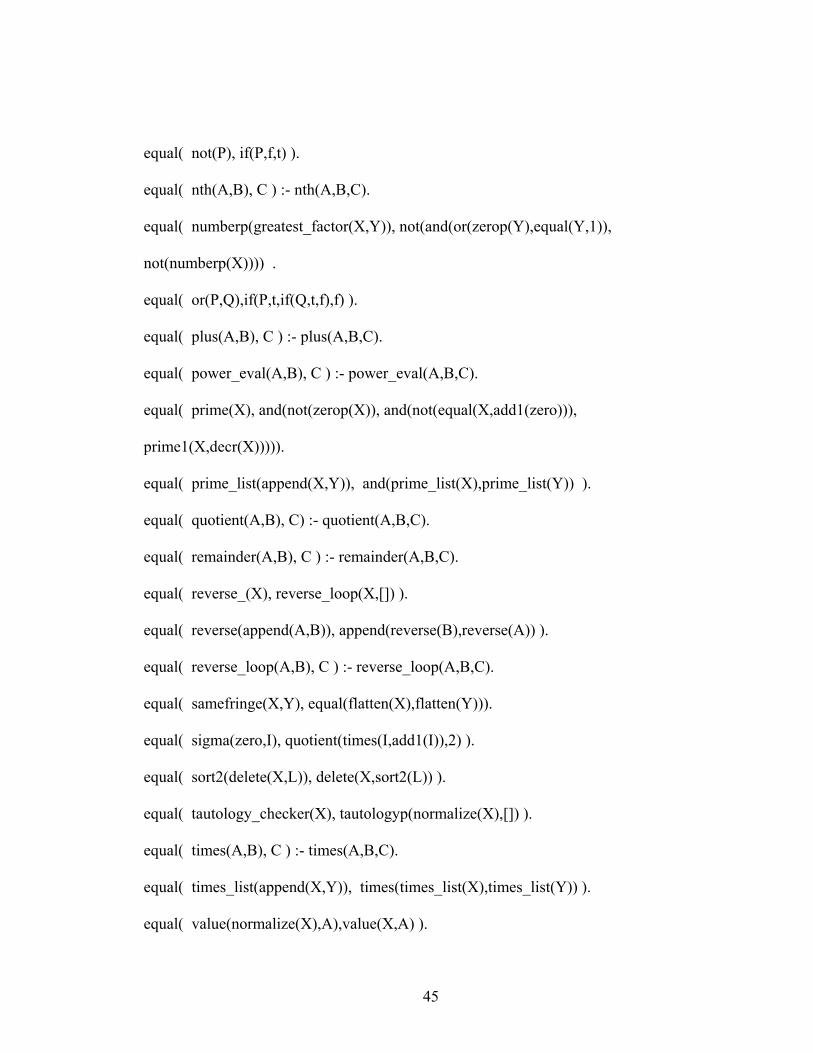
40

:-write('use -h8000 -t1000 in BinProlog'),nl.

/*

% generated: 20 November 1989

% option(s):

% boyer

% Evan Tick (from Lisp version by R. P. Gabriel)

% November 1985

% prove arithmetic theorem

*/

go:- statistics(global_stack,[H1,_]), statistics(runtime,_), run_boyer,

statistics(runtime,[_,Y]),statistics(global_stack,[H2,_]),H is H2 - H1,

write('BMARK_boyer time: '), write(time(Y)+heap(H)), nl.

run_boyer:- wff(Wff), write('rewriting...'),nl, rewrite(Wff,NewWff), write('proving...'),nl,

tautology(NewWff,[],[]).

wff(implies(and(implies(X,Y), and(implies(Y,Z), and(implies(Z,U), implies(U,W)))),

implies(X,W))) :-X = f(plus(plus(a,b),plus(c,zero))),

Y = f(times(times(a,b),plus(c,d))),

Z = f(reverse(append(append(a,b),[]))),

U = equal(plus(a,b),difference(x,y)),

W = lessp(remainder(a,b),member(a,length(b))).

41

tautology(Wff,Tlist,Flist) :-(truep(Wff,Tlist) -> true

;falsep(Wff,Flist) -> fail

;Wff = if(If,Then,Else) ->

(truep(If,Tlist) -> tautology(Then,Tlist,Flist)

;falsep(If,Flist) -> tautology(Else,Tlist,Flist)

;tautology(Then,[If|Tlist],Flist), % both must hold

tautology(Else,Tlist,[If|Flist])

)

),!.

rewrite(Atom,Atom) :-atomic(Atom),!.

rewrite(Old,New) :-functor(Old,F,N),functor(Mid,F,N), rewrite_args(N,Old,Mid),

( equal(Mid,Next), % should be ->, but is compiler smart

rewrite(Next,New) % enough to generate cut for -> ?

; New=Mid

),!.

rewrite_args(0,_,_) :- !.

rewrite_args(N,Old,Mid) :- N1 is N-1, arg(N,Old,OldArg), arg(N,Mid,MidArg),

rewrite(OldArg,MidArg), rewrite_args(N1,Old,Mid).

truep(t,_) :- !.

42

truep(Wff,Tlist) :- member_chk(Wff,Tlist).

falsep(f,_) :- !.

falsep(Wff,Flist) :- member_chk(Wff,Flist).

member_chk(X,[X|_]) :- !.

member_chk(X,[_|T]) :- member_chk(X,T).

equal( and(P,Q), if(P,if(Q,t,f),f) ).

equal( append(append(X,Y),Z), append(X,append(Y,Z)) ).

equal( assignment(X,append(A,B)), if(assignedp(X,A), assignment(X,A),

assignment(X,B))).

equal( assume_false(Var,Alist), cons(cons(Var,f),Alist) ).

equal( assume_true(Var,Alist), cons(cons(Var,t),Alist) ).

equal( boolean(X), or(equal(X,t),equal(X,f)) ).

equal( car(gopher(X)), if(listp(X), car(flatten(X)), zero) ).

equal( compile(Form), reverse(codegen(optimize(Form),[])) ).

equal( count_list(Z,sort_lp(X,Y)), plus(count_list(Z,X), count_list(Z,Y)) ).

equal( countps_(L,Pred), countps_loop(L,Pred,zero) ).

equal( difference(A,B), C ) :- difference(A,B,C).

equal( divides(X,Y), zerop(remainder(Y,X)) ).

equal( dsort(X), sort2(X) ).

equal( eqp(X,Y), equal(fix(X),fix(Y)) ).

equal( equal(A,B), C ) :- eq(A,B,C).

equal( even1(X), if(zerop(X),t,odd(decr(X))) ).

43

equal( exec(append(X,Y),Pds,Envrn), exec(Y,exec(X,Pds,Envrn),Envrn) ).

equal( exp(A,B), C ) :- exp(A,B,C).

equal( fact_(I),fact_loop(I,1)).

equal( falsify(X),falsify1(normalize(X),[])).

equal( fix(X),if(numberp(X),X,zero)).

equal( flatten(cdr(gopher(X))), if(listp(X),cdr(flatten(X)),cons(zero,[]))).

equal( gcd(A,B),C) :- gcd(A,B,C).

equal( get(J,set(I,Val,Mem)),if(eqp(J,I),Val,get(J,Mem))).

equal( greatereqp(X,Y),not(lessp(X,Y)) ).

equal( greatereqpr(X,Y),not(lessp(X,Y))).

equal( greaterp(X,Y), lessp(Y,X)).

equal( if(if(A,B,C),D,E),if(A,if(B,D,E),if(C,D,E))).

equal( iff(X,Y),and(implies(X,Y),implies(Y,X))).

equal( implies(P,Q),if(P,if(Q,t,f),t)).

equal( last(append(A,B)), if(listp(B),last(B), if(listp(A),cons(car(last(A))),B))).

equal( length(A),B) :- mylength(A,B).

equal( lesseqp(X,Y),not(lessp(Y,X))).

equal( lessp(A,B),C) :- lessp(A,B,C).

equal( listp(gopher(X)), listp(X)).

equal( mc_flatten(X,Y),append(flatten(X),Y)).

equal( meaning(A,B), C ) :- meaning(A,B,C).

equal( member_chk(A,B), C ) :- mymember(A,B,C).

44

equal( not(P), if(P,f,t) ).

equal( nth(A,B), C ) :- nth(A,B,C).

equal( numberp(greatest_factor(X,Y)), not(and(or(zerop(Y),equal(Y,1)),

not(numberp(X)))) .

equal( or(P,Q),if(P,t,if(Q,t,f),f) ).

equal( plus(A,B), C ) :- plus(A,B,C).

equal( power_eval(A,B), C ) :- power_eval(A,B,C).

equal( prime(X), and(not(zerop(X)), and(not(equal(X,add1(zero))),

prime1(X,decr(X))))).

equal( prime_list(append(X,Y)), and(prime_list(X),prime_list(Y)) ).

equal( quotient(A,B), C) :- quotient(A,B,C).

equal( remainder(A,B), C ) :- remainder(A,B,C).

equal( reverse_(X), reverse_loop(X,[]) ).

equal( reverse(append(A,B)), append(reverse(B),reverse(A)) ).

equal( reverse_loop(A,B), C ) :- reverse_loop(A,B,C).

equal( samefringe(X,Y), equal(flatten(X),flatten(Y))).

equal( sigma(zero,I), quotient(times(I,add1(I)),2) ).

equal( sort2(delete(X,L)), delete(X,sort2(L)) ).

equal( tautology_checker(X), tautologyp(normalize(X),[]) ).

equal( times(A,B), C ) :- times(A,B,C).

equal( times_list(append(X,Y)), times(times_list(X),times_list(Y)) ).

equal( value(normalize(X),A),value(X,A) ).

45

equal( zerop(X), or(equal(X,zero),not(numberp(X)))).

difference(X, X, zero) :- !.

difference(plus(X,Y), X, fix(Y)) :- !.

difference(plus(Y,X), X, fix(Y)) :- !.

difference(plus(X,Y), plus(X,Z), difference(Y,Z)) :- !.

difference(plus(B,plus(A,C)), A, plus(B,C)) :- !.

difference(add1(plus(Y,Z)), Z, add1(Y)) :- !.

difference(add1(add1(X)), 2, fix(X)).

eq(plus(A,B), zero, and(zerop(A),zerop(B))) :- !.

eq(plus(A,B), plus(A,C), equal(fix(B),fix(C))) :- !.

eq(zero, difference(X,Y),not(lessp(Y,X))) :- !.

eq(X, difference(X,Y),and(numberp(X), and(or(equal(X,zero), zerop(Y))))) :- !.

eq(times(X,Y), zero, or(zerop(X),zerop(Y))) :- !.

eq(append(A,B), append(A,C), equal(B,C)) :- !.

eq(flatten(X), cons(Y,[]), and(nlistp(X),equal(X,Y))) :- !.

eq(greatest_factor(X,Y),zero, and(or(zerop(Y),equal(Y,1)), equal(X,zero))) :- !.

eq(greatest_factor(X,_),1, equal(X,1)) :- !.

eq(Z, times(W,Z), and(numberp(Z), or(equal(Z,zero), equal(W,1)))) :- !.

eq(X, times(X,Y), or(equal(X,zero), and(numberp(X),equal(Y,1)))) :- !.

eq(times(A,B), 1, and(not(equal(A,zero)), and(not(equal(B,zero)), and(numberp(A),

46

and(numberp(B), and(equal(decr(A),zero), equal(decr(B),zero))))))) :- !.

eq(difference(X,Y), difference(Z,Y),if(lessp(X,Y), not(lessp(Y,Z)),if(lessp(Z,Y),

not(lessp(Y,X)), equal(fix(X),fix(Z))))) :- !.

eq(lessp(X,Y), Z, if(lessp(X,Y), equal(t,Z), equal(f,Z))).

exp(I, plus(J,K), times(exp(I,J),exp(I,K))) :- !.

exp(I, times(J,K), exp(exp(I,J),K)).

gcd(X, Y, gcd(Y,X)) :- !.

gcd(times(X,Z), times(Y,Z), times(Z,gcd(X,Y))).

mylength(reverse(X),length(X)).

mylength(cons(_,cons(_,cons(_,cons(_,cons(_,cons(_,X7)))))),

plus(6,length(X7))).

lessp(remainder(_,Y), Y, not(zerop(Y))) :- !.

lessp(quotient(I,J), I, and(not(zerop(I)), or(zerop(J), not(equal(J,1))))) :- !.

lessp(remainder(X,Y), X, and(not(zerop(Y)), and(not(zerop(X)), not(lessp(X,Y))))) :- !.

lessp(plus(X,Y), plus(X,Z), lessp(Y,Z)) :- !.

lessp(times(X,Z), times(Y,Z), and(not(zerop(Z)), lessp(X,Y))) :- !.

lessp(Y, plus(X,Y), not(zerop(X))) :- !.

lessp(length(delete(X,L)), length(L), member(X,L)).

47

meaning(plus_tree(append(X,Y)),A, plus(meaning(plus_tree(X),A),

meaning(plus_tree(Y),A))) :- !.

meaning(plus_tree(plus_fringe(X)),A, fix(meaning(X,A))) :- !.

meaning(plus_tree(delete(X,Y)),A, if(member(X,Y),difference(meaning(plus_tree(Y),A),

meaning(X,A)), meaning(plus_tree(Y),A))).

mymember(X,append(A,B),or(member(X,A),member(X,B))) :- !.

mymember(X,reverse(Y),member(X,Y)) :- !.

mymember(A,intersect(B,C),and(member(A,B),member(A,C))).

nth(zero,_,zero).

nth([],I,if(zerop(I),[],zero)).

nth(append(A,B),I,append(nth(A,I),nth(B,difference(I,length(A))))).

plus(plus(X,Y),Z, plus(X,plus(Y,Z))) :- !.

plus(remainder(X,Y), times(Y,quotient(X,Y)), fix(X)) :- !.

plus(X,add1(Y), if(numberp(Y), add1(plus(X,Y)), add1(X))).

power_eval(big_plus1(L,I,Base),Base,

plus(power_eval(L,Base),I)) :- !.

power_eval(power_rep(I,Base),Base, fix(I)) :- !.

48

power_eval(big_plus(X,Y,I,Base),Base, plus(I,plus(power_eval(X,Base),

power_eval(Y,Base)))) :- !.

power_eval(big_plus(power_rep(I,Base), power_rep(J,Base), zero, Base),

Base, plus(I,J)).

quotient(plus(X,plus(X,Y)),2,plus(X,quotient(Y,2))).

quotient(times(Y,X),Y,if(zerop(Y),zero,fix(X))).

remainder(_, 1,zero) :- !.

remainder(X, X,zero) :- !.

remainder(times(_,Z),Z,zero) :- !.

remainder(times(Y,_),Y,zero).

reverse_loop(X,Y, append(reverse(X),Y)) :- !.

reverse_loop(X,[], reverse(X) ).

times(X, plus(Y,Z), plus(times(X,Y),times(X,Z)) ) :- !.

times(times(X,Y),Z, times(X,times(Y,Z)) ) :- !.

times(X, difference(C,W),difference(times(C,X),times(W,X))) :- !.

times(X, add1(Y), if(numberp(Y), plus(X,times(X,Y)), fix(X)) ).

49

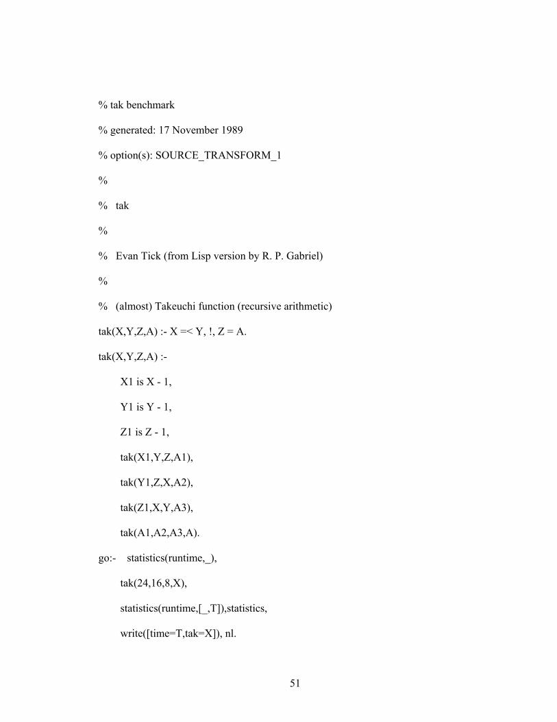
APPENDIX D

TAK.PL

50

% tak benchmark

% generated: 17 November 1989

% option(s): SOURCE_TRANSFORM_1

%

% tak

%

% Evan Tick (from Lisp version by R. P. Gabriel)

%

% (almost) Takeuchi function (recursive arithmetic)

tak(X,Y,Z,A) :- X =< Y, !, Z = A.

tak(X,Y,Z,A) :-

X1 is X - 1,

Y1 is Y - 1,

Z1 is Z - 1,

tak(X1,Y,Z,A1),

tak(Y1,Z,X,A2),

tak(Z1,X,Y,A3),

tak(A1,A2,A3,A).

go:- statistics(runtime,_),

tak(24,16,8,X),

statistics(runtime,[_,T]),statistics,

write([time=T,tak=X]), nl.

51

APPENDIX E

INPUT FILE TO PAJEK GENERATOR “INPUT.NET”

52

*Vertices 59

58 "statistics(go1(1000000,go2(10000,or(((no = yes) , !(0) , do_body(true)),no =

no,or(((no = yes) , !(0) , do_body(true)),no = no,true)))))"

59 "go1(1000000,go2(10000,or(((no = yes) , !(0) , do_body(true)),no = no,or(((no = yes)

, !(0) , do_body(true)),no = no,true))))"

55 go1(1000000,go2(10000,or(((no = yes) , !(0) , do_body(true)),no = no,or(((no = yes) ,

!(0) , do_body(true)),no = no,true))))

57 go2(10000,or(((no = yes) , !(0) , do_body(true)),no = no,or(((no = yes) , !(0) ,

do_body(true)),no = no,true)))

52 go2(10000,or(((no = yes) , !(0) , do_body(true)),no = no,or(((no = yes) , !(0) ,

do_body(true)),no = no,true)))

54 or(((no = yes) , !(0) , do_body(true)),no = no,or(((no = yes) , !(0) , do_body(true)),no

= no,true))

48 or(((no = yes) , !(0) , do_body(true)),no = no,or(((no = yes) , !(0) , do_body(true)),no

= no,true))



31 true

30 no = no

25 no = no

27 no

26 no

53

13 no

29 ((no = yes) , !(0) , do_body(true))


24 (!(0) , do_body(true))


21 do_body(true)

17 do_body(true)

18 true

20 !(0)

15 !(0)

16 0

23 no = yes

12 no = yes

14 yes

50 no = no

45 no = no

47 no

46 no

33 no




54


41 do_body(true)

37 do_body(true)

38 true

40 !(0)

35 !(0)

36 0

43 no = yes

32 no = yes

34 yes

53 10000

56 1000000

1 '$answer'(topcall(go))


6 topcall(go)

7 topcall(go)

8 go

2 ('$answer'(topcall(go)) :- topcall(go))

4 topcall(go)

9 topcall(go)

10 go


55

*Edges

3 5

9 10

4 9

2 4

2 3

7 8

6 7

5 6

1 5

32 34

32 33

43 32

35 36

40 35

37 38

41 37

39 41

39 40

44 39

42 44

42 43

56

49 42

46 33

45 47

45 46

50 45

12 14

12 13

23 12

15 16

20 15

17 18

21 17

19 21

19 20

24 19

22 24

22 23

29 22

26 13

25 27

25 26

30 25

57

28 31

28 30

28 29

51 28

48 51

48 50

48 49

54 48

52 54

52 53

57 52

55 57

55 56

59 55

58 59

58

APPENDIX F

MATLAB FORMULAE

59

Partial Marking

plot(x1/(0.1)^0.71,y,'-',y,y,'-')

plot(x2/(0.2)^0.46,y,'-',y,y,'-')

plot(x3/(0.3)^0.28,y,'-',y,y,'-')

plot(x4/(0.4)^0.16,y,'-',y,y,'-')

plot(x5/(0.5)^0.09,y,'-',y,y,'-')

plot(x6/(0.6)^0.06,y,'-',y,y,'-')

plot(x7/(0.7)^0.03,y,'-',y,y,'-')

plot(x8/(0.8)^0.02,y,'-',y,y,'-')

plot(x9/(0.9)^0.01,y,'-',y,y,'-')

i)plot(x1/(0.1)^0.71,y,'-',x2/(0.2)^0.46,y,'-',x3/(0.3)^0.28,y,'-',x4/(0.4)^0.16,y,'-'

,x5/(0.5)^0.09,y,'-',x6/(0.6)^0.06,y,'-',x7/(0.7)^0.03,y,'-',x8/(0.8)^0.02,y,'-

',x9/(0.9)^0.01,y,'-',y,y,'-')

ii) plot(x1,h,'-',x2,h,'-',x3,h,'-',x4,h,'-',x5,h,'-',x6,h,'-',x7,h,'-',x8,h,'-',x9,h,'-',y,h,'-')

ii) plot(x1,y,'-',x2,y,'-',x3,y,'-',x4,y,'-',x5,y,'-',x6,y,'-',x7,y,'-',x8,y,'-',x9,y,'-',y,y,'-')

60

With out using previous Partial

Markings

plot(x1/(0.1)^0.75,y,'-',y,y,'-')

plot(x2/(0.2)^0.67,y,'-',y,y,'-')

plot(x3/(0.3)^0.61,y,'-',y,y,'-')

plot(x4/(0.4)^0.56,y,'-',y,y,'-')

plot(x5/(0.5)^0.53,y,'-',y,y,'-')

plot(x6/(0.6)^0.50,y,'-',y,y,'-')

plot(x7/(0.7)^0.49,y,'-',y,y,'-')

plot(x8/(0.8)^0.49,y,'-',y,y,'-')

plot(x9/(0.9)^0.49,y,'-',y,y,'-')

plot(x1/(0.1)^0.75,y,'-',x2/(0.2)^0.67,y,'-',x3/(0.3)^0.61,y,'-',x4/(0.4)^0.56,y,'-'

,x5/(0.5)^0.53,y,'-',x6/(0.6)^0.50,y,'-',x7/(0.7)^0.49,y,'-',x8/(0.8)^0.49,y,'-

',x9/(0.9)^0.49,y,'-',y,y,'-')

61

REFERENCE LIST:

[1] Paul Tarau. Inference and Computation Mobility with Jinni. In K.R.Apt, V.W. Marek,

and M. Truszczynski, editors, The Logic Programming Paradigm: a 25 Year Perspective,

pages 33-48.Springer, 1999. ISBN 3-540-65463-1.

[2] Nancy Glenn. Statistical Learning Techniques for intelligent memory management,

Department of statistics, University of South Carolina

[3]Overview of different memory management techniques are available at

http://www.memorymanagement.org/articles/

[4] http://logic.csci.unt.edu/tarau/priv/pub/papers/IMPLEMENTATION_MEMORY/

[5] Douglas B. West, “Introduction to Graph Theory”, Prentice-Hall Inc, 1996. pages

409-415.

[6] Joel Spencer, Random Graphs, IMA Summer Graduate Student Program at Ohio State

University, August 23-27, 1993.

[7] William Aiello, Fan Chung, Linyan Lu, a random graph model for massive graphs,

Poceedings of the Thirtysecond Annual ACM Symposium on Theory of Computing

2000.

[8] S.R.Kumar, P.Raphavan, S.Rajagopalan and A.Tomkins, Trawling the web for

emerging cyber communities, Proceedings of the 8th world wide Web Conference,

Toronto, 1999

[9] Martin Hirzel, Johannes Henkel, Amer Diwan and Michael Hind, Understanding the

Connectivity of Heap Objects.

62

http://www.memorymanagement.org/articles/

[10] Introduction to Monte Carlo Methods, Computational science Education Project

1991, 1992, 1993, 1994, 1995

[11] V. Batagelj, A. Mrvar: Pajek - Program for Large Network Analysis. Home page

http://vlado.fmf.uni-lj.si/pub/networks/pajek/.

[12] Information about MATLAB® can be obtained at:

http://www.mathworks.com/access/helpdesk/help/techdoc/learn_matlab/learn_matlab.sht

ml

[13] B.Bollobas, Random Graphs, Academic Press, 1985

[14] Documentation of Jinni prolog can be obtained from the following link:

http://www.binnetcorp.com/download/jinnidemo/JinniUserGuide.html

[15] Hongsuda Tangmunarunkit, Ramesh Govindan, Sugih Jamin. Network Toplogy

Generators: Degree-Based vs. Structural, SIGCOMM’02, Aug 19-23, Pittsburg,

Pennsylvania.

[16] http://www.statsoftinc.com/textbook/stathome.html

63

http://vlado.fmf.uni-lj.si/pub/networks/pajek/

Intelligent Memory Management Heuristics

Documents

Transcript of Intelligent Memory Management Heuristics