Intelligent Market-Making in Artificial Financial

Markets

by

Sanmay Das

A.B. Computer Science

Harvard College, 2001

Submitted to the Department of Electrical Engineering and Computer

Sciencein partial fulfillment of the requirements for the degree of

Master of Science in Computer Science and Engineering

at the

MASSACHUSETTS INSTITUTE OF TECHNOLOGY

June 2003

c© Massachusetts Institute of Technology 2003. All rights reserved.

Author . . . . . . . . . . . . . . . . . . . . . . . . . . . . . . . . . . . . . . . . . . . . . . . . . . . . . . . . . . . . . .Department of Electrical Engineering and Computer Science

April 9, 2003

Certified by. . . . . . . . . . . . . . . . . . . . . . . . . . . . . . . . . . . . . . . . . . . . . . . . . . . . . . . . . .

Tomaso PoggioEugene McDermott Professor

Thesis Supervisor

Accepted by . . . . . . . . . . . . . . . . . . . . . . . . . . . . . . . . . . . . . . . . . . . . . . . . . . . . . . . . .Arthur C. Smith

Chairman, Department Committee on Graduate Students

2

Intelligent Market-Making in Artificial Financial Markets

by

Sanmay Das

Submitted to the Department of Electrical Engineering and Computer Scienceon April 9, 2003, in partial fulfillment of the

requirements for the degree ofMaster of Science in Computer Science and Engineering

Abstract

This thesis describes and evaluates a market-making algorithm for setting prices infinancial markets with asymmetric information, and analyzes the properties of artifi-cial markets in which the algorithm is used. The core of our algorithm is a techniquefor maintaining an online probability density estimate of the underlying value of astock. Previous theoretical work on market-making has led to price-setting equa-tions for which solutions cannot be achieved in practice, whereas empirical work onalgorithms for market-making has focused on sets of heuristics and rules that lacktheoretical justification. The algorithm presented in this thesis is theoretically justi-fied by results in finance, and at the same time flexible enough to be easily extendedby incorporating modules for dealing with considerations like portfolio risk and com-petition from other market-makers. We analyze the performance of our algorithmexperimentally in artificial markets with different parameter settings and find thatmany reasonable real-world properties emerge. For example, the spread increases inresponse to uncertainty about the true value of a stock, average spreads tend to behigher in more volatile markets, and market-makers with lower average spreads per-form better in environments with multiple competitive market-makers. In addition,the time series data generated by simple markets populated with market-makers usingour algorithm replicate properties of real-world financial time series, such as volatilityclustering and the fat-tailed nature of return distributions, without the need to specifyexplicit models for opinion propagation and herd behavior in the trading crowd.

Thesis Supervisor: Tomaso PoggioTitle: Eugene McDermott Professor

3

4

Acknowledgments

First of all, I’d like to thank Tommy for being a terrific advisor, patient when results

don’t come and excited when they do. Many others have contributed to this work.

Andrew Lo has been a valuable source of direction. Adlar Kim has been a great

partner in research, always willing to listen to ideas, no matter how half-baked. This

thesis benefited from numerous conversations with Sayan Mukherjee on learning and

Ranen Das, Nicholas Chan and Tarun Ramadorai on finance. Jishnu Das provided

help in getting past a sticking point in the density estimation technique. I’d also

like to thank everyone at CBCL, especially Adlar, Sayan, Tony, Luis, Thomas, Gadi,

Mary Pat, Emily and Casey for making lab a fun and functional place to be, and my

parents and brothers for their love and support.

This thesis describes research done at the Center for Biological & Computational

Learning, which is in the Department of Brain & Cognitive Sciences at MIT and

which is affiliated with the McGovern Institute of Brain Research and with the Ar-

tificial Intelligence Laboratory. I was partially supported by an MIT Presidential

Fellowship for 2001–2002. In addition, this research was sponsored by grants from

Merrill-Lynch, National Science Foundation (ITR/IM) Contract No. IIS-0085836 and

National Science Foundation (ITR/SYS) Contract No. IIS-0112991. Additional sup-

port was provided by the Center for e-Business (MIT), DaimlerChrysler AG, Eastman

Kodak Company, Honda R&D Co., Ltd., The Eugene McDermott Foundation, and

The Whitaker Foundation.

5

6

Contents

1 Introduction 13

1.1 Background . . . . . . . . . . . . . . . . . . . . . . . . . . . . . . . . 13

1.1.1 Market Microstructure and Market-Making . . . . . . . . . . . 14

1.1.2 Artificial Markets . . . . . . . . . . . . . . . . . . . . . . . . . 15

1.1.3 Multi-Agent Simulations and Machine Learning . . . . . . . . 17

1.2 Contributions . . . . . . . . . . . . . . . . . . . . . . . . . . . . . . . 18

1.3 Overview . . . . . . . . . . . . . . . . . . . . . . . . . . . . . . . . . . 19

2 The Market-Making Algorithm 21

2.1 Market Microstructure Background . . . . . . . . . . . . . . . . . . . 21

2.2 Detailed Market Model . . . . . . . . . . . . . . . . . . . . . . . . . . 23

2.3 The Market-Making Algorithm . . . . . . . . . . . . . . . . . . . . . 25

2.3.1 Derivation of Bid and Ask Price Equations . . . . . . . . . . . 26

2.3.2 Accounting for Noisy Informed Traders . . . . . . . . . . . . . 27

2.3.3 Approximately Solving the Equations . . . . . . . . . . . . . . 29

2.3.4 Updating the Density Estimate . . . . . . . . . . . . . . . . . 30

3 Inventory Control, Profit Motive and Transaction Prices 33

3.1 A Naive Market-Maker . . . . . . . . . . . . . . . . . . . . . . . . . . 33

3.2 Experimental Framework . . . . . . . . . . . . . . . . . . . . . . . . . 34

3.3 Inventory Control . . . . . . . . . . . . . . . . . . . . . . . . . . . . . 34

3.4 Profit Motive . . . . . . . . . . . . . . . . . . . . . . . . . . . . . . . 38

3.4.1 Increasing the Spread . . . . . . . . . . . . . . . . . . . . . . . 38

7

3.4.2 Active Learning . . . . . . . . . . . . . . . . . . . . . . . . . . 40

3.4.3 Competitive Market-Making . . . . . . . . . . . . . . . . . . . 42

3.5 The Effects of Volatility . . . . . . . . . . . . . . . . . . . . . . . . . 44

3.6 Accounting for Jumps . . . . . . . . . . . . . . . . . . . . . . . . . . 45

3.7 Time Series Properties of Transaction Prices . . . . . . . . . . . . . . 46

4 Conclusions and Future Work 51

4.1 Summary . . . . . . . . . . . . . . . . . . . . . . . . . . . . . . . . . 51

4.2 Future Directions . . . . . . . . . . . . . . . . . . . . . . . . . . . . . 53

8

List of Figures

2-1 An example limit order book . . . . . . . . . . . . . . . . . . . . . . . 22

2-2 Example of the true value over time . . . . . . . . . . . . . . . . . . . 25

2-3 The evolution of the market-maker’s probability density estimate with

noisy informed traders (above) and perfectly informed traders (below) 31

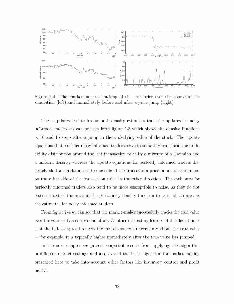
2-4 The market-maker’s tracking of the true price over the course of the

simulation (left) and immediately before and after a price jump (right) 32

3-1 Step function for inventory control and the underlying sigmoid function 35

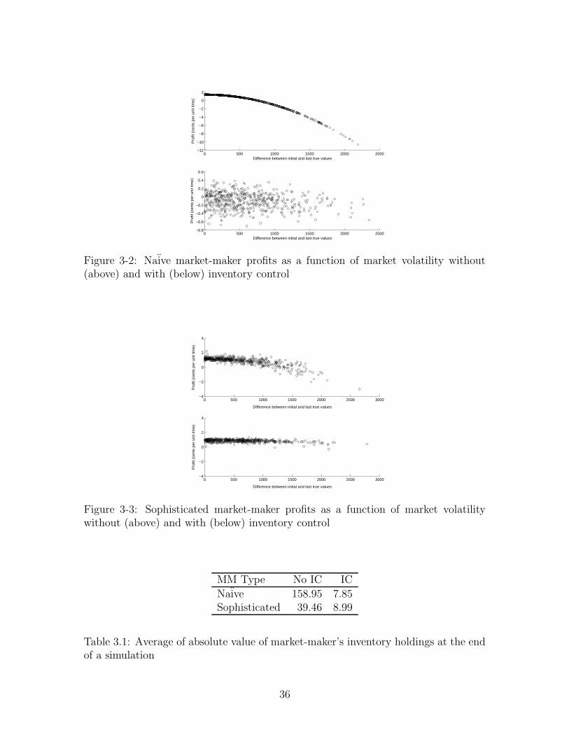
3-2 Naive market-maker profits as a function of market volatility without

(above) and with (below) inventory control . . . . . . . . . . . . . . . 36

3-3 Sophisticated market-maker profits as a function of market volatility

without (above) and with (below) inventory control . . . . . . . . . . 36

3-4 Market-maker profits as a function of increasing the spread . . . . . . 39

3-5 Market-maker profits with noisy informed traders and perfectly in-

formed traders . . . . . . . . . . . . . . . . . . . . . . . . . . . . . . . 40

3-6 Standardized log returns over time . . . . . . . . . . . . . . . . . . . 47

3-7 Leptokurtic distribution of absolute standardized log returns . . . . . 48

3-8 Autocorrelation of absolute returns . . . . . . . . . . . . . . . . . . . 49

3-9 Autocorrelation of absolute returns on a log-log scale for lags of 1-100 49

3-10 Autocorrelation of raw returns . . . . . . . . . . . . . . . . . . . . . . 50

9

10

List of Tables

3.1 Average of absolute value of market-maker’s inventory holdings at the

end of a simulation . . . . . . . . . . . . . . . . . . . . . . . . . . . . 36

3.2 Correlation between market volatility and market-maker profit for market-

makers with and without inventory control . . . . . . . . . . . . . . . 37

3.3 Average profit (in cents per time period) for market-makers with and

without inventory control . . . . . . . . . . . . . . . . . . . . . . . . 37

3.4 Average profit (in cents per time period) for market-makers with and

without randomization in the sampling strategy . . . . . . . . . . . . 41

3.5 Market-maker profits (in cents per time period) and average number

of trades in simulations lasting 50,000 time steps in monopolistic and

competitive environments . . . . . . . . . . . . . . . . . . . . . . . . 43

3.6 Market-maker average spreads (in cents) and profits (in cents per time

period) as a function of the standard deviation of the jump process . 44

3.7 Market-maker average spreads (in cents) and profits (in cents per time

period) as a function of the probability of a jump occurring at any

point in time . . . . . . . . . . . . . . . . . . . . . . . . . . . . . . . 45

3.8 Average profit (in cents per time period) and loss of expectation for

market-makers using different parameters for recentering the probabil-

ity distribution . . . . . . . . . . . . . . . . . . . . . . . . . . . . . . 46

11

12

Chapter 1

Introduction

In the last decade there has been a surge of interest within the finance community in

describing equity markets through computational agent models. At the same time,

financial markets are an important application area for the fields of agent-based mod-

eling and machine learning, since agent objectives and interactions tend to be more

clearly defined, both practically and mathematically, in these markets than in other

areas. In this thesis we consider market-making agents who play important roles in

stock markets and who need to optimize their pricing decisions under conditions of

asymmetric information while taking into account other considerations such as port-

folio risk. This setting provides a rich and dynamic testbed for ideas from machine

learning and artificial intelligence and simultaneously allows one to draw insights

about the behavior of financial markets.

1.1 Background

The important concepts presented and derived in this thesis are drawn from both

the finance and artificial intelligence literatures. The set of problems we are study-

ing with respect to the dynamics of market behavior has been studied in the market

microstructure and artificial markets communities, while the approach towards mod-

eling financial markets and market-making presented here is based on techniques

from artificial intelligence such as non-parametric probability density estimation and

13

multi-agent based simulation.

1.1.1 Market Microstructure and Market-Making

The detailed study of equity markets necessarily involves examination of the processes

and outcomes of asset exchange in markets with explicit trading rules. Price formation

in markets occurs through the process of trading. The field of market microstructure

is concerned with the specific mechanisms and rules under which trades take place in

a market and how these mechanisms impact price formation and the trading process.

O’Hara [23] and Madhavan [21] present excellent surveys of the market microstructure

literature.

Asset markets can be structured in different ways. The simplest type of market is

a standard double auction market, in which competitive buyers and sellers enter their

prices and matching prices result in the execution of trades [13]. Some exchanges

like the New York Stock Exchange (NYSE) employ market-makers for each stock in

order to ensure immediacy and liquidity. The market-maker for each stock on the

NYSE is obligated to continuously post two-sided quotes (a bid quote and an ask

quote). Each quote consists of a size and a price, and the market-maker must honor a

market buy or sell order of that size (or below) at the quoted price, so that customer

buy and sell orders can be immediately executed. The NYSE employs monopolistic

market-makers. Only one market-maker is permitted per stock, and that market-

maker is strictly regulated by the exchange to ensure market quality. Market quality

can be measured in a number of different ways. One commonly used measure is the

average size of the bid-ask spread (the difference between the bid and ask prices). An

exchange like the NASDAQ (National Association of Securities Dealers Automated

Quotation System) allows multiple market-makers for each stock with less regulation,

in the expectation that good market quality will arise from competition between the

market-makers1.

Theoretical analysis of microstructure has traditionally been an important part of

the literature. Models in theoretical finance share some important aspects that we use

1A detailed exposition of the different types of market structures is given by Schwartz [26].

14

throughout this thesis. For example, the ability to model order arrival as a stochastic

process, following Garman [14] and Glosten and Milgrom [15], is important for the

derivations of optimal pricing strategies presented here. The basic concepts of how

market-makers minimize risk through inventory control and how this process affects

prices in the market are also used in framing the market-maker’s decision problem

and deriving pricing strategies (see, for example, Amihud and Mendelson [1]).

The main problem with theoretical microstructure models is that they are typically

restricted to simple, stylized cases with rigid assumptions about trader behavior.

There are two major alternative approaches to the study of microstructure. These

are the experimental markets approach ([11, 17] inter alia) and the artificial markets

approach ([7, 10, 25] inter alia). The work presented in this thesis falls into the

artificial markets approach, and we briefly review the artificial markets literature.

1.1.2 Artificial Markets

Artificial markets are market simulations populated with artificially intelligent elec-

tronic agents that fill the roles of traders. These agents can use heuristics, rules,

and machine learning techniques to make trading decisions. Many artificial market

simulations also use an evolutionary approach, with agents entering and leaving the

market, and agent trading strategies evolving over time. Most research in artificial

markets centers on modeling financial markets from the bottom up as structures that

emerge from the interactions of individual agents.

Computational modeling of markets allows for the opportunity to push beyond the

restrictions of traditional theoretical models of markets through the use of computa-

tional power. At the same time, the artificial markets approach allows a fine-grained

level of experimental control that is not available in real markets. Thus, data obtained

from artificial market experiments can be compared to the predictions of theoretical

models and to data from real-world markets, and the level of control allows one to

examine precisely which settings and conditions lead to the deviations from theoreti-

cal predictions usually seen in the behavior of real markets. LeBaron [18] provides a

summary of some of the early work on agent-based computational finance.

15

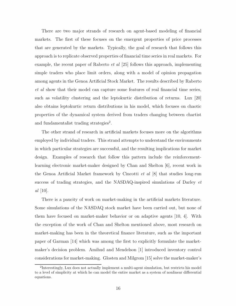
There are two major strands of research on agent-based modeling of financial

markets. The first of these focuses on the emergent properties of price processes

that are generated by the markets. Typically, the goal of research that follows this

approach is to replicate observed properties of financial time series in real markets. For

example, the recent paper of Raberto et al [25] follows this approach, implementing

simple traders who place limit orders, along with a model of opinion propagation

among agents in the Genoa Artificial Stock Market. The results described by Raberto

et al show that their model can capture some features of real financial time series,

such as volatility clustering and the leptokurtic distribution of returns. Lux [20]

also obtains leptokurtic return distributions in his model, which focuses on chaotic

properties of the dynamical system derived from traders changing between chartist

and fundamentalist trading strategies2.

The other strand of research in artificial markets focuses more on the algorithms

employed by individual traders. This strand attempts to understand the environments

in which particular strategies are successful, and the resulting implications for market

design. Examples of research that follow this pattern include the reinforcement-

learning electronic market-maker designed by Chan and Shelton [6], recent work in

the Genoa Artificial Market framework by Cincotti et al [8] that studies long-run

success of trading strategies, and the NASDAQ-inspired simulations of Darley et

al [10].

There is a paucity of work on market-making in the artificial markets literature.

Some simulations of the NASDAQ stock market have been carried out, but none of

them have focused on market-maker behavior or on adaptive agents [10, 4]. With

the exception of the work of Chan and Shelton mentioned above, most research on

market-making has been in the theoretical finance literature, such as the important

paper of Garman [14] which was among the first to explicitly formulate the market-

maker’s decision problem. Amihud and Mendelson [1] introduced inventory control

considerations for market-making. Glosten and Milgrom [15] solve the market-maker’s

2Interestingly, Lux does not actually implement a multi-agent simulation, but restricts his modelto a level of simplicity at which he can model the entire market as a system of nonlinear differentialequations.

16

decision problem under information asymmetry. This thesis extends theoretical mod-

els of market-making and implements them within the context of our artificial market.

1.1.3 Multi-Agent Simulations and Machine Learning

From the perspective of computer science, both multi-agent based simulation and

machine learning have increased their importance as subfields of artificial intelligence

over the last decade or so. As LeBaron [18] points out, financial markets are one of

the most important applications for agent-based modeling because issues of price and

information aggregation and dissemination tend to be sharper in financial settings,

where objectives of agents are usually clearer. Further, the availability of massive

amounts of real financial data allows for comparison with the results of agent-based

simulations.

In general, work on artificial markets incorporates either learning or evolution as

a means of adding dynamic structure to the markets. In settings where the availabil-

ity of information is a crucial aspect of market dynamics, adaptive agents who can

incorporate information and learn from market trends become important players. For

example, techniques from classification [22] can be used to predict price movements

for chartist agents, and explicit Bayesian learning can be used by decision-theoretic

agents to incorporate all available information into the decision-making process. Tech-

niques for tracking a moving parameter [5, 3] are useful in estimating the possibly

changing fundamental value of a stock. The price-setting process of market-making

essentially forms a control layer on top of an estimation problem, leading to tradeoffs

similar to the exploration-exploitation tradeoffs often found in reinforcement learning

contexts [28]. Competitive market-making poses its own set of problems that need to

be addressed using game-theoretic analysis and considerations of collaborative and

competitive agent behavior [12].

17

1.2 Contributions

The research described in this thesis serves as a bridge in the literature between the

purely theoretical work on optimal market-making techniques such as the paper of

Glosten and Milgrom [15], which we use for the theoretical underpinnings of this work,

and the more realistic experimental work on market-making that has been carried

out by Chan [7] and Darley et al [10]. We derive an algorithm for price setting that

is theoretically grounded in the optimal price-setting equations derived by Glosten

and Milgrom, and generalize the technique to more realistic market settings. The

algorithm has many desirable properties in the market environments in which we

have tested it, such as the ability to make profits while maintaining a low bid-ask

spread.

The market-making algorithm presented in this thesis is flexible enough to allow

it to be adapted to different settings, such as monopolistic or competitive market-

making settings, and extended with other modules. We present extensive experimen-

tal results for the market-making algorithm and extensions such as inventory control.

We analyze the effects of competition, volatility and jumps in the underlying value

on market-maker profits, the bid-ask spread and the execution of trades.

The data from simulations of markets in which market-makers use the algorithms

developed in this thesis yield interesting insights into the behavior of price processes.

We compare the time series properties of the price data generated by our simulations

to the known characteristics of such data from real markets and find that we are

able to replicate some important features of real financial time series, such as the

leptokurtic distribution of returns, without postulating explicit, complex models of

agent interaction and herd behavior3 as has previously been done in the literature [20,

25]4.

3Some explicit models of herd behavior are presented in the economics literature by Banerjee [2],Cont and Bouchaud [9] and Orlean [24] inter alia.

4It is worth noting that the true value process can induce behavior (especially following a jump)similar to that induced by herd behavior through informed traders all buying or selling simultane-ously based on superior information. However, the mechanism is a much weaker assumption thanthe assumption of explicit imitative behavior or mimetic contagion.

18

1.3 Overview

This thesis is structured as follows. Chapter 2 provides necessary background in-

formation on market microstructure, introduces the market model, and derives the

equations for price setting that the main market-making algorithm uses. It also

presents in detail the cornerstone of the market-making algorithm, a technique for

online probability density estimation that the market-maker uses to track the true

underlying value of the stock.

Chapter 3 describes the practical implementation of the algorithm by taking into

account the market-maker’s profit motive and desire to control portfolio risk. This

chapter also presents empirical analysis of the algorithm in various different market

settings, including settings with multiple competitive market-makers, and details the

important time series properties of our model. Chapter 4 summarizes the contribu-

tions of this thesis and suggests avenues for future work.

19

20

Chapter 2

The Market-Making Algorithm

2.1 Market Microstructure Background

The artificial market presented in this thesis is largely based on ideas from the the-

oretical finance literature1. Here we briefly review some of the important concepts.

A stock is assumed to have an underlying true value (or fundamental value) at all

points in time. The price at which the stock trades is not necessarily close to this

value at all times (for example, during a bubble, the stock trades at prices consid-

erably higher than its true value). There are two principal kinds of traders in the

market. Informed traders (sometimes referred to as fundamentalist traders) are those

who know (or think they know) the true value of the stock and base their decisions

on the assumption that the transaction price will revert to the true value. Informed

traders will try to buy when they think a stock is undervalued by the market price,

and will try to sell when they think a stock is overvalued by the market price. Some-

times it is useful to think of informed traders as those possessing inside information.

Uninformed traders (also referred to as noise traders) trade for reasons exogenous to

the market model. Usually they are modeled as buying or selling stock at random

(one psychological model is traders who buy or sell for liquidity reasons). Other mod-

els of traders are often mentioned in the literature, such as chartists who attempt to

predict the direction of stock price movement, but we are not concerned with such

1For a detailed introduction to the basic concepts of market microstructure see Schwartz [26].

21

Buy Orders Sell OrdersSize Price ($) Price ($) Sizex1 23.20 23.28 y1

x2 23.18 23.30 y2

x3 23.15 24.25 y3

x4 23.00

Figure 2-1: An example limit order book

models of trading in this thesis.

There are two main types of orders in stock markets. These are market orders

and limit orders. A market order specifies the size of the order in shares and whether

the order is a buy or sell order. A limit order also specifies a price at which the trader

placing the order is willing to buy or sell. Market orders are guaranteed execution

but not price. That is, in placing a market order a trader is assured that it will

get executed within a short amount of time at the best market price, but is not

guaranteed what that price will be. Limit orders, on the other hand, are guaranteed

price but not execution. That is, they will only get executed at the specified price,

but this may never happen if a matching order is not found.

A double auction market in the context of stocks can be defined as a market in

which limit orders and market orders are present and get executed against each other

at matching prices. The limit orders taken together form an order book, in which the

buy orders are arranged in decreasing order of price, while the sell orders are arranged

in increasing order of price (see figure 2-1 for an example). Orders that match are

immediately executed, so the highest buy order remaining must have a lower price

than the lowest ask order remaining. Market orders, when they arrive, are executed

against the best limit order on the opposite side. So, for example, a market buy order

would get executed against the best limit sell order currently on the book.

Double auction markets are effective when there is sufficient liquidity in the stock.

There must be enough buy and sell orders for incoming market orders to be guaranteed

immediate execution at prices that are not too far away from the prices at which

transactions executed recently. Sometimes these conditions are not met, typically

22

for stocks that do not trade in high volume (for obvious reasons) and immediately

following particularly favorable or unfavorable news (when everyone wants to be either

on the buy or sell side of the market, leading to huge imbalances).

Market-makers are traders designated by markets to maintain immediacy and liq-

uidity in transactions. Market-makers are obligated to continuously post two-sided

quotes (bid (for buying) and ask (for selling) quotes) and honor these quotes. Apart

from providing immediacy and liquidity to order execution, market-makers are also

expected to smooth the transition when the price of a stock jumps dramatically, so

that traders do not believe they received unfair executions, and to maintain a rea-

sonable bid-ask spread. Exchanges with monopolistic market-makers like the NYSE

monitor the performance of market-makers on these categories, while markets like

NASDAQ use multiple market-makers and expect good market quality to arise from

competition between market-makers.

2.2 Detailed Market Model

The market used in this thesis is a discrete time dealer market with only one stock.

The market-maker sets bid and ask prices (Pb and Pa respectively) at which it is

willing to buy or sell one unit of the stock at each time period (when necessary we

denote the bid and ask prices at time period i as P i

band P i

a). If there are multiple

market-makers, the market bid and ask prices are the maximum over each dealer’s

bid price and the minimum over each dealer’s ask price. All transactions occur with

the market-maker taking one side of the trade and a member of the trading crowd

(henceforth a “trader”) taking the other side of the trade.

The stock has a true underlying value (or fundamental value) V i at time period

i. All market makers are informed of V 0 at the beginning of a simulation, but do

not receive any direct information about V after that2. At time period i, a single

trader is selected from the trading crowd and allowed to place either a (market) buy

2That is, the only signals a market-maker receives about the true value of the stock are throughthe buy and sell orders placed by the trading crowd.

23

or (market) sell order for one unit of the stock. There are two types of traders in the

market, uninformed traders and informed traders. An uninformed trader will place

a buy or sell order for one unit at random if selected to trade. An informed trader

who is selected to trade knows V i and will place a buy order if V i > P ia, a sell order

if V i < P i

band no order if P i

b≤ V i ≤ P i

a.

In addition to perfectly informed traders, we also allow for the presence of noisy

informed traders. A noisy informed trader receives a signal of the true price W i =

V i + η(0, σW ) where η(0, σW ) represents a sample from a normal distribution with

mean 0 and variance σ2W

. The noisy informed trader believes this is the true value of

the stock, and places a buy order if W i > P ia, a sell order if W i < P i

band no order if

P i

b≤ W i ≤ P i

a.

The true underlying value of the stock evolves according to a jump process. At

time i + 1, with probability p, a jump in the true value occurs3. When a jump

occurs, the value changes according to the equation V i+1 = V i+ω(0, σ) where ω(0, σ)

represents a sample from a normal distribution with mean 0 and variance σ2. Thus,

jumps in the value can be more substantial at a given point in time than those in

a unit random walk model such as the one used by Chan and Shelton [6], but the

probability of a change in the true value in our model is usually significantly lower

than the probability of a change in the true value in unit random walk models.

This model of the evolution of the true value corresponds to the notion of the

true value evolving as a result of occasional news items. For example, jumps can be

due to information received about the company itself (like an earnings report), or

information about a particular sector of the market, or even information that affects

the market as a whole. When a jump occurs, the informed traders are placed in

an advantageous position. The periods immediately following jumps are the periods

in which informed traders can trade most profitably, because the information they

have on the true value has not been disseminated to the market yet, and the market

maker is not informed of changes in the true value and must estimate these through

orders placed by the trading crowd. The market-maker will not update prices to the

3p is typically small, of the order of 1 in 1000 in most of our simulations

24

0 1 2 3 4 5 6 7 8 9 10

x 104

996

997

998

999

1000

1001

1002

1003

1004

Time Period

Tru

e P

rice

($)

Figure 2-2: Example of the true value over time

neighborhood of the new true value for some period of time immediately following a

jump in the true value, and informed traders can exploit the information asymmetry.

2.3 The Market-Making Algorithm

The most important feature of the market-making model presented in this thesis is

that the market-maker attempts to track the true value over time by maintaining a

probability distribution over possible true values and updating the distribution when

it receives signals from the market buy or sell orders that traders place. The true

value and the market-maker’s prices together induce a probability distribution on the

orders that arrive in the market. The market-maker’s task is to maintain an online

probabilistic estimate of the true value, which is itself a moving target.

Glosten and Milgrom [15] analyze the setting of bid and ask prices so that the

market maker enforces a zero profit condition. The zero profit condition corresponds

to the Nash equilibrium in a setting with competitive market-makers (or, more gen-

erally in any competitive price-setting framework [12]). Glosten and Milgrom suggest

that the market maker should set Pb = E[V |Sell] and Pa = E[V |Buy]. Our market-

making algorithm computes these expectations using the probability density function

being estimated.

25

Various layers of complexity can be added on top of the basic algorithm. For

example, minimum and maximum conditions can be imposed on the spread, and an

inventory control mechanism could form another layer after the zero-profit condition

prices are decided. Thus, the central part of our algorithm relates to the density

estimation itself. We will describe the density estimation technique in detail before

addressing other possible factors that market-makers can take into account in deciding

how to set prices. For simplicity of presentation, we neglect noisy informed traders in

the initial derivation, and present the updated equations for taking them into account

later.

2.3.1 Derivation of Bid and Ask Price Equations

In order to estimate the expectation of the underlying value, it is necessary to compute

the conditional probability that V = x given that a particular type of order is received.

Taking market sell orders as the example:

E[V |Sell] =

∫

∞

0

x Pr(V = x|Sell) dx (2.1)

Since we want to explicitly compute these values and are willing to make approx-

imations for this reason, we discretize the X-axis into intervals, with each interval

representing one cent. Then we get:

E[V |Sell] =

Vi=Vmax∑

Vi=Vmin

Vi Pr(V = Vi|Sell)

Applying Bayes’ rule and simplifying:

E[V |Sell] =

Vi=Vmax∑

Vi=Vmin

Vi Pr(Sell|V = Vi) Pr(V = Vi)

Pr(Sell)

26

Since Pb is set by the market maker to E[V |Sell] and the a priori probabilities of

both a buy and a sell order are equal to 1/2:

Pb = 2

Vi=Vmax∑

Vi=Vmin

Vi Pr(Sell|V = Vi) Pr(V = Vi) (2.2)

Since Vmin < Pb < Vmax,

Pb = 2

Vi=Pb∑

Vi=Vmin

Vi Pr(Sell|V = Vi) Pr(V = Vi) + 2

Vi=Vmax∑

Vi=Pb+1

Vi Pr(Sell|V = Vi) Pr(V = Vi)

(2.3)

The importance of splitting up the sum in this manner is that the term Pr(Sell|V =

Vi) is constant within each sum, because of the influence of informed traders. An

uninformed trader is equally likely to sell whatever the market maker’s bid price. On

the other hand, an informed trader will never sell if V > Pb. Suppose the proportion

of informed traders in the trading crowd is α. Then Pr(Sell|V ≤ Pb) = 1

2+ 1

2α and

Pr(Sell|V > Pb) = 1

2− 1

2α. Then the above equation reduces to:

Pb = 2

(

Vi=Pb∑

Vi=Vmin

(1

2+

1

2α)Vi Pr(V = Vi) +

Vi=Vmax∑

Vi=Pb+1

(1

2−

1

2α)Vi Pr(V = Vi)

)

(2.4)

Using a precisely parallel argument, we can derive the expression for the market-

maker’s ask price:

Pa = 2

(

Vi=Pa∑

Vi=Vmin

(1

2−

1

2α)Vi Pr(V = Vi) +

Vi=Vmax∑

Vi=Pa+1

(1

2+

1

2α)Vi Pr(V = Vi)

)

(2.5)

2.3.2 Accounting for Noisy Informed Traders

An interesting feature of the probabilistic estimate of the true value is that the prob-

ability of buying or selling is the same conditional on V being smaller than or greater

than a certain amount. For example, Pr(Sell|V = Vi, Vi ≤ Pb) is a constant, inde-

pendent of V . If we assume that all informed traders receive noisy signals, with the

27

noise normally distributed with mean 0 and variance σ2W

, and, as before, α is the

proportion of informed traders in the trading crowd, then equation 2.3 still applies.

Now the probabilities Pr(Sell|V = Vi) are no longer determined solely by whether

Vi ≤ Pb or Vi > Pb. Instead, the new equations are:

Pr(Sell|V = Vi, Vi ≤ Pb) = (1 − α)1

2+ α Pr(η(0, σW ) ≤ (Pb − Vi)) (2.6)

and:

Pr(Sell|V = Vi, Vi > Pb) = (1 − α)1

2+ α Pr(η(0, σW ) ≥ (Vi − Pb)) (2.7)

The second term in the first equation reflects the probability that an informed

trader would sell if the fundamental value were less than the market-maker’s bid

price. This will occur as long as W = V + η(0, σW ) ≤ Pb. Similarly, the second term

in the second equation reflects the same probability, except with the assumption that

V > Pb.

We can compute the conditional probabilities for buy orders equivalently:

Pr(Buy|V = Vi, Vi ≤ Pa) = (1 − α)1

2+ α Pr(η(0, σW ) ≥ (Pa − Vi)) (2.8)

and:

Pr(Buy|V = Vi, Vi > Pa) = (1 − α)1

2+ α Pr(η(0, σW ) ≤ (Vi − Pa)) (2.9)

We can substitute these conditional probabilities back into both the fixed point

equations and the density update rule used by the market-maker. First of all, com-

28

bining equations 2.3, 2.6 and 2.7, we get:

Pb = 2

Vi=Pb∑

Vi=Vmin

(1

2−

1

2α + α Pr(η(0, σW ) ≤ (Pb − Vi)))Vi Pr(V = Vi) +

2

Vi=Vmax∑

Vi=Pb+1

(1

2−

1

2α + α Pr(η(0, σW ) ≥ (Vi − Pb)))Vi Pr(V = Vi) (2.10)

Similarly, for the ask price:

Pa = 2

Vi=Pa∑

Vi=Vmin

(1

2−

1

2α + α Pr(η(0, σW ) ≥ (Pa − Vi)))Vi Pr(V = Vi) +

2

Vi=Vmax∑

Vi=Pa+1

(1

2−

1

2α + α Pr(η(0, σW ) ≤ (Vi − Pa)))Vi Pr(V = Vi) (2.11)

2.3.3 Approximately Solving the Equations

A number of problems arise with the analytical solution of these discrete equations

for setting the bid and ask prices. Most importantly, we have not yet specified the

probability distribution for priors on V , and any reasonably complex solution leads

to a form that makes analytical solution infeasible. Secondly, the values of Vmin and

Vmax are undetermined. And finally, actual solution of these fixed point equations

must be approximated in discrete spaces. We solve each of these problems in turn to

construct an empirical solution to the problem and then present experimental results

in the next chapter.

We assume that the market-making agent is aware of the true value at time 0,

and from then onwards the true value infrequently receives random shocks (or jumps)

drawn from a normal distribution (the variance of which is known to the agent). Our

market-maker constructs a vector of prior probabilities on various possible values of

V as follows.

If the initial true value is V0 (when rounded to an integral value in cents), then

the agent constructs a vector going from V0 − 4σ to V0 + 4σ − 1 to contain the prior

value probabilities. The probability that V = V0 − 4σ + i is given by the ith value

29

in this vector4. The vector is initialized by setting the ith value in the vector to∫

−4σ+i+1

−4σ+iN (0, σ) dx where N is the normal density function in x with specified mean

and variance. The reason for selecting 4σ as the range is that it contains 99.9% of

the density of the normal, which we assume to be a reasonable number of entries.

The vector is also maintained in a normalized state at all times so that the entire

probability mass for V lies within it.

The fixed point equations 2.10 and 2.11 are approximately solved by using the

result from Glosten and Milgrom that Pb ≤ E[V ] ≤ Pa and then, to find the bid

price, for example, cycling from E[V] downwards until the difference between the left

and right hand sides of the equation stops decreasing. The fixed point real-valued

solution must then be closest to the integral value at which the distance between the

two sides of the equation is minimized.

2.3.4 Updating the Density Estimate

The market-maker receives probabilistic signals about the true value. With perfectly

informed traders, each signal says that with a certain probability, the true value is

lower (higher) than the bid (ask) price. With noisy informed traders, the signal

differentiates between different possible true values depending on the market-maker’s

bid and ask quotes. Each time that the market-maker receives a signal about the true

value by receiving a market buy or sell order, it updates the posterior on the value of

V by scaling the distributions based on the type of order. The Bayesian updates are

easily derived. For example, for Vi ≤ Pa and market buy orders:

Pr(V = Vi|Buy) =Pr(Buy|V = Vi) Pr(V = Vi)

Pr(Buy)

The prior probability V = Vi is known from the density estimate, the prior probability

of a buy order is 1/2, and Pr(Buy|V = Vi, Vi ≤ Pa) can be computed from equation

2.8. We can compute the posterior similarly for each of the cases.

4It is important to note that the true value can be a real number, but for all practical purposesit ends up getting truncated to the floor of that number.

30

−4 −3 −2 −1 0 1 2 3 4 0

0.02

0.04

0.06

0.08

0.1

0.12

Standard deviations away from the mean (true value = −0.56)

Prob

abilit

y

0 steps5 steps10 steps15 steps

−4 −3 −2 −1 0 1 2 3 4 0

0.01

0.02

0.03

0.04

0.05

0.06

Standard deviations away from the mean (true value = −0.84)

Prob

abilit

y

0 steps5 steps10 steps15 steps

Figure 2-3: The evolution of the market-maker’s probability density estimate withnoisy informed traders (above) and perfectly informed traders (below)

An interesting note is that in the case of perfectly informed traders, the signal only

specifies that the true value is higher or lower than some price, and not how much

higher or lower. In that case, the update equations are as follows. If a market buy

order is received, this is a signal that with probability 1

2(1−α)+α = 1

2+ 1

2α, V > Pa.

Similarly, if a market sell order is received, the signal indicates that with probability

1

2+ 1

2α, V < Pb. In the former case, all probabilities for V = Vi, Vi > Pa are multiplied

by 1

2+ 1

2α, while all the other discrete probabilities are multiplied by 1 − ( 1

2+ 1

2α).

Similarly, when a sell order is received, all probabilities for V = Vi, Vi < Pb are

multiplied by 1

2+ 1

2α, and all the remaining discrete probabilities are multiplied by

1 − (1

2+ 1

2α) before renormalizing.

31

0 0.5 1 1.5 2 2.5 3 3.5 4 4.5 5

x 104

988

990

992

994

996

998

1000

1002

Time Period

Tru

e V

alue

($)

0 0.5 1 1.5 2 2.5 3 3.5 4 4.5 5

x 104

985

990

995

1000

1005

Time Period

Exp

ecte

d V

alue

($)

1800 1810 1820 1830 1840 1850 1860 1870 1880 1890 1900

999.4

999.6

999.8

1000

1000.2

Time Period

Pric

e ($

)

1800 1810 1820 1830 1840 1850 1860 1870 1880 1890 19000

0.02

0.04

0.06

0.08

0.1

Time Period

Spr

ead

($)

True ValueBid PriceAsk Price

Figure 2-4: The market-maker’s tracking of the true price over the course of thesimulation (left) and immediately before and after a price jump (right)

These updates lead to less smooth density estimates than the updates for noisy

informed traders, as can be seen from figure 2-3 which shows the density functions

5, 10 and 15 steps after a jump in the underlying value of the stock. The update

equations that consider noisy informed traders serve to smoothly transform the prob-

ability distribution around the last transaction price by a mixture of a Gaussian and

a uniform density, whereas the update equations for perfectly informed traders dis-

cretely shift all probabilities to one side of the transaction price in one direction and

on the other side of the transaction price in the other direction. The estimates for

perfectly informed traders also tend to be more susceptible to noise, as they do not

restrict most of the mass of the probability density function to as small an area as

the estimates for noisy informed traders.

From figure 2-4 we can see that the market-maker successfully tracks the true value

over the course of an entire simulation. Another interesting feature of the algorithm is

that the bid-ask spread reflects the market-maker’s uncertainty about the true value

— for example, it is typically higher immediately after the true value has jumped.

In the next chapter we present empirical results from applying this algorithm

in different market settings and also extend the basic algorithm for market-making

presented here to take into account other factors like inventory control and profit

motive.

32

Chapter 3

Inventory Control, Profit Motive

and Transaction Prices

3.1 A Naive Market-Maker

At this stage, it is necessary to introduce a simple algorithm for market-making.

There are two main reasons to study such an algorithm. First, it helps to elucidate

the effects of some extensions to the main algorithm presented in the last chapter

(which we shall sometimes refer to as the “sophisticated” algorithm), and second,

it provides a basis for comparison. This naive market-maker “surrounds” the last

transaction price with its bid and ask quotes while maintaining a fixed spread at all

times. At the first time period, the market-maker knows the initial true value and

sets its bid and ask quotes around that price. So, for example, if the last transaction

price was Ph and the market-maker uses a fixed spread δ, it would set its bid and ask

quotes at Ph −δ

2and Ph + δ

2respectively.

Given that we do not consider transaction sizes in this thesis, the above algorithm

is actually surprisingly effective for market-making, as it adjusts its prices upwards or

downwards depending on the kinds of orders entering the market. The major problem

with the algorithm is that it is incapable of adjusting its spread to react to market

conditions or to competition from other market-makers, so, as we shall demonstrate,

it does not perform as well (relatively speaking) in competitive environments or under

33

volatile market conditions as algorithms that take market events into account more

explicitly.

3.2 Experimental Framework

Unless specified otherwise, it can be assumed that all simulations take place in a

market populated by noisy informed traders and uninformed traders. The noisy

informed traders receive a noisy signal of the true value of the stock with the noise

term being drawn from a Gaussian distribution with mean 0 and standard deviation

5 cents. The standard deviation of the jump process for the stock is 50 cents, and

the probability of a jump occurring at any time step is 0.005. The market-maker is

informed of when a jump occurs, but not of the size or direction of the jump. The

market-maker uses an inventory control function (defined below) and increases the

spread by lowering the bid price and raising the ask price by a fixed amount (this is

done to ensure profitability and is also explained below). We report average results

from 50 simulations, each lasting 50,000 time steps.

3.3 Inventory Control

Stoll analyzes dealer costs in conducting transactions and divides them into three

categories [27]. These three categories are portfolio risk, transaction costs and the

cost of asymmetric information. In the model we have presented so far, following

Glosten and Milgrom [15], we have assumed that transactions have zero execution

cost and developed a pricing mechanism that explicitly attempts to set the spread to

account for the cost of asymmetric information.

A realistic model for market-making necessitates taking portfolio risk into account

as well, and controlling inventory in setting bid and ask prices. In the absence of

consideration of trade size and failure conditions, portfolio risk should affect the

placement of the bid and ask prices, but not the size of the spread1 [1, 27, 16]. If the

1One would expect spread to increase with the trade size.

34

0 5 10 15 20 25 30 35 40 45 500

0.5

1

1.5

2

2.5

3

3.5

4

4.5

5

Absolute value of stock inventory

Abs

olut

e va

lue

of p

rice

adju

stm

ent (

cent

s)

Figure 3-1: Step function for inventory control and the underlying sigmoid function

market-maker has a long position in the stock, minimizing portfolio risk is achieved by

lowering both bid and ask prices (effectively making it harder for the market-maker

to buy stock and easier for it to sell stock), and if the market-maker has a short

position, inventory is controlled by raising both bid and ask prices.

Inventory control can be incorporated into the architecture of our market-making

algorithm by using it as an adjustment parameter applied after bid and ask prices

have been determined by equations 2.10 and 2.11. An example of the kind of function

we can use to determine the amount of the shift is a sigmoid function. The motivation

for using a sigmoid function is to allow for an initial gradual increase in the impact of

inventory control on prices, followed by a steeper increase as inventory accumulates,

while simultaneously bounding the upper limit by which inventory control can play

a factor in price setting. Of course, the upper bound and slope of the sigmoid can be

adjusted according to the qualities desired in the function.

For our simulations, we use an inventory control function that uses the floor of a

real valued sigmoid function with a ceiling of 5 cents as the integer price adjustment

(in cents). The step function for the adjustment and the underlying sigmoid are

shown in figure 3-1.

Figure 3-2 is a scatter plot that shows the effects of using the above inventory

control function for a naive market-maker using a δ value of 8 cents (note that the Y

35

0 500 1000 1500 2000 2500−12

−10

−8

−6

−4

−2

0

2

Difference between initial and last true values

Pro

fit (

cent

s pe

r un

it tim

e)

0 500 1000 1500 2000 2500−0.8

−0.6

−0.4

−0.2

0

0.2

0.4

0.6

Difference between initial and last true values

Pro

fit (

cent

s pe

r un

it tim

e)

Figure 3-2: Naive market-maker profits as a function of market volatility without(above) and with (below) inventory control

0 500 1000 1500 2000 2500 3000−4

−2

0

2

4

Difference between initial and last true values

Pro

fit (

cent

s pe

r un

it tim

e)

0 500 1000 1500 2000 2500 3000−4

−2

0

2

4

Difference between initial and last true values

Pro

fit (

cent

s pe

r un

it tim

e)

Figure 3-3: Sophisticated market-maker profits as a function of market volatilitywithout (above) and with (below) inventory control

MM Type No IC IC

Naive 158.95 7.85Sophisticated 39.46 8.99

Table 3.1: Average of absolute value of market-maker’s inventory holdings at the endof a simulation

36

MM Type No IC IC

Naive −0.9470 −0.1736Sophisticated −0.7786 −0.3452

Table 3.2: Correlation between market volatility and market-maker profit for market-makers with and without inventory control

MM Type No IC IC

Naive −0.1672 −0.1033Sophisticated 0.8372 0.8454

Table 3.3: Average profit (in cents per time period) for market-makers with andwithout inventory control

axes are on different scales for the two parts of the figure). Figure 3-3 shows the effects

for a market-maker using the sophisticated algorithm2. Table 3.1 shows the average

absolute value of inventory held by the market-maker at the end of each simulation

for the different cases. The figures use the absolute value of the difference between

last true value and initial true value as a proxy for estimating market volatility, as

this difference provides a measure of how much a large inventory could affect profit

for a particular simulation. 500 simulations were run for each experiment, and 70%

of the traders were noisy informed traders, while the rest were uninformed.

The results in figures 3-2 and 3-3 and tables 3.2 and 3.3 demonstrate that without

inventory control, market-maker profits are highly correlated with volatility, and the

inventory control module we have suggested successfully removes the dependence of

profit on volatility without reducing expected profit. The differences in profit for the

inventory control and no inventory control cases are not statistically significant for

either the naive or the sophisticated market-maker. In fact, it is somewhat surpris-

ing that average profit is not reduced by inventory control, since adding inventory

control is similar to adding additional constraints to an optimization problem. This

effect could be due to the fact that our algorithm is not in fact performing exact

2For this experiment, the market-maker was modified to increase the spread beyond the zeroprofit condition by lowering the bid price by 3 cents and increasing the ask price by 3 cents. Themotivation for this is to use a profitable market-maker, as will become clear in the next section, andto perform a fair comparison with a naive market-maker that uses a fixed spread of 8 cents.

37

optimization, and the inventory control module may help to adjust prices in the cor-

rect direction in volatile markets. Another interesting fact is that the sophisticated

market-making algorithm is less susceptible to the huge losses that the naive market-

maker incurs in very volatile market environments, even without inventory control.

This suggests that the sophisticated algorithm is adapting to different environments

more successfully than the naive algorithm.

3.4 Profit Motive

The zero-profit condition of Glosten and Milgrom is expected from game theoretic

considerations when multiple competitive dealers are making markets in the same

stock. However, since our method is an approximation scheme, the zero profit method

is unlikely to truly be zero-profit. Further, the market-maker is not always in a per-

fectly competitive scenario where it needs to restrict the spread as much as possible.

In this section, we investigate some possibilities for increasing the spread to ensure

profitability conditions for the market-making algorithm.

3.4.1 Increasing the Spread

The simplest solution to the problem of making profit is to increase the spread by

pushing the bid and ask prices apart after the zero-profit bid and ask prices have been

computed using the density estimate obtained by the market-making algorithm. The

major effect of this on the density estimation technique is that the signals the market-

maker receives and uses to update its density estimate are determined by transaction

prices, which are in turn determined by the bid and ask prices the market-maker has

set. The precise values of the bid and ask prices are quite important to the sampling

of the distribution on trades induced by the true value.

Figure 3-4 shows the profit obtained by a single monopolistic market-maker in

markets with different percentages of noisy informed traders. The numbers on the X

axis show the amount (in cents) that is subtracted from (added to) the zero-profit bid

(ask) price in order to push the spread apart (we will refer to this number as the shift

38

0 1 2 3 4 5 6 7 8 9 10−1

−0.5

0

0.5

1

1.5

Amount added to ask price and subtracted from bid price (cents)

Mar

ket−

mak

er p

rofit

per

uni

t tim

e (c

ents

)

50% inf70% inf90% inf

Figure 3-4: Market-maker profits as a function of increasing the spread

factor). It is important to note that market-makers can make reasonable profits with

low average spreads – an example is given at the end of the section on competitive

market-making.

With lower spreads, most of the market-maker’s profits come from the noise factor

of the informed traders, whereas with a higher spread, most of the market-maker’s

profits come from the trades of uninformed traders. Different percentages of in-

formed traders lead to differently shaped curves. With only 50% of the traders being

informed, the market-maker’s profit keeps increasing with the size of the spread. How-

ever, increasing the spread beyond a point is counterproductive if there are enough

noisy informed traders in the markets, because then the market-maker’s prices are

far enough away from the true value that even the noise factor cannot influence the

informed traders to make trades. With 90% of the traders being informed, a global

maximum (at least for reasonable spreads) is attained with a low spread, while with

70% of the traders being informed, a local maximum is attained with a fairly low

spread, although the larger number of uninformed traders allows for larger profits

with rather large spreads.

Another point worth mentioning is that the market-maker’s probability density

estimates tend to be more concentrated with more noisy informed traders in the

markets, because each trade provides more information. This leads to the empirical

39

0 1 2 3 4 5 6 7 8 9 10−1.5

−1

−0.5

0

0.5

1

Amount added to ask price and subtracted from bid price (cents)

Mar

ket−

mak

er p

rofit

per

uni

t tim

e (c

ents

)

70% noisy informed70% perfectly informed

Figure 3-5: Market-maker profits with noisy informed traders and perfectly informedtraders

results being closer to theoretical predictions. For example, the prices leading to zero

profit for the 70% informed and 90% informed cases fall between the 0 and 1 points

on the X axis, which is close to what one would expect from the theory, whereas with

perfectly informed traders zero profit is not obtained without using a large spread.

Figure 3-5 compares the profits obtained by the market-maker with 70% noisy

informed traders as opposed to 70% perfectly informed traders. In the latter case,

there is no advantage to be gained by having a smaller spread as there is with noisy

informed traders. However, the market-maker’s inability to make any profit even

with a high spread seems surprising. This is partly attributable to the fact that

the point at which the distribution is sampled is more important in the perfectly

informed case because the signals only inform the market-maker of the probabilities

that the true value is greater than or less than the last transaction price, instead

of smoothly morphing points around the last transaction price by a mixture of a

Gaussian distribution and a uniform distribution.

3.4.2 Active Learning

The above observation on how the smoothing effect of noisy informed traders on the

posterior distribution helps to maintain, in some senses, a “good” density estimate

40

Bid/Ask Adjustment Perfectly Informed Noisy Informed4 -0.7382 0.80754r -0.5119 0.5594

Table 3.4: Average profit (in cents per time period) for market-makers with andwithout randomization in the sampling strategy

points us in an interesting direction for the case of perfectly informed traders. We

can see from figure 3-5 that, counterintuitively, profits increase slowly with increasing

spread. Since the market-maker sets “controls” at Pb and Pa, it may not be getting

“good” samples for estimating the probability density for values in the region between

Pb and Pa, which is the most important part of the distribution, since the true value

probably lies in that range.

One way of dealing with this problem is to occasionally sample from the distri-

bution between Pb and Pa by not increasing the spread and just using the zero-profit

condition prices some percentage of the time. We tested the effectiveness of this

method in markets with informed traders constituting 50% of the trading crowd, and

the market-maker decreasing the bid price and increasing the ask price by 4 cents. In

the randomized case, the market-maker increased the spread 60% of the time, leaving

it untouched otherwise. The results from this experiment are shown in table 3.4.

“4r” represents the randomized algorithm, and we can see that it outperforms

the non-randomized version (in fact, it also outperforms versions that use higher

spreads) in markets with perfectly informed traders. The same does not hold true

for markets with noisy informed traders, where the loss incurred by not pushing the

spread up at each opportunity dominates any benefits gained from improving the

density estimate. This is because of the smoother nature of the noisy estimate, as

discussed above. There may be an interesting connection between this behavior and

the “exploration-exploitation” tradeoff as thought of in reinforcement learning [28]

— a market-maker willing to sacrifice profits temporarily in order to improve its

estimate can make more profit in the long term. The online nature of the problem

decrees that the probability of sampling more aggressively by not increasing the spread

cannot be smoothly decreased over time, but perhaps more sophisticated algorithms

41

for sampling the important areas of the distribution might help performance even

more in terms of profit in the perfectly informed case. Perhaps some of the ideas

for sampling from the distribution more effectively can be adapted to the noisy case.

This is an interesting direction for future work.

3.4.3 Competitive Market-Making

The most important aspect of competitive market-making within the framework in

which we view it is that market-makers are not guaranteed to execute trades just by

being in the market. Instead the highest bid price quoted by any market-maker and

the lowest ask price quoted by any market-maker become the effective market bid-ask

quotes, and the market-makers compete with each other for trades. A market-maker

who does not make a sufficient number of trades will lose out to a market-maker who

makes substantially more trades even if the latter makes less profit per trade.

This effect is particularly obvious in the first experiment shown in table 3.5. In this

experiment, two market-makers who both use the market-making algorithm presented

in this thesis compete with each other, with the difference that one uses a shift factor

of 2 and the other a shift factor of 3 for increasing the spread after the zero-profit

bid and ask prices have been determined. If neither were using an inventory control

mechanism, the market-maker using a shift factor of 3 would in fact make no trades,

because the market-maker using a shift factor of 2 would always have the inside

quotes for both the bid and the ask. The addition of inventory control allows the

market-maker using a shift factor of 3 to make some trades, but this market-maker

makes considerably less profit than the one using a shift factor of 2. In a monopolistic

environment the market-maker using a shift factor of 3 outperforms the market-maker

using a shift factor of 2 and the difference in magnitude of executed trades is not as

large.

It is interesting to compare two different strategies for market-making in competi-

tive and monopolistic environments. The naive market-making algorithm outperforms

the sophisticated algorithm in a monopolistic framework with 70% of the traders be-

ing perfectly informed and the rest uninformed. However, it is outperformed by the

42

70% noisy informed tradersCompetitive Monopolistic

MM Type Profit # Trades Profit # TradesSoph (shift = 2) 0.6039 38830 0.6216 39464Soph (shift = 3) 0.0157 594 0.8655 34873

70% noisy informed tradersCompetitive Monopolistic

MM Type Profit # Trades Profit # TradesNaive (spread = 8) -0.8020 17506 -0.0840 35176Soph (shift = 3) 0.7687 20341 0.8655 34873

70% perfectly informed tradersCompetitive Monopolistic

MM Type Profit # Trades Profit # TradesNaive (spread = 8) -0.9628 12138 -0.5881 23271Soph (shift = 3) -0.6379 16331 -0.8422 27581

Table 3.5: Market-maker profits (in cents per time period) and average number oftrades in simulations lasting 50,000 time steps in monopolistic and competitive envi-ronments

sophisticated algorithm in the same environment when they are in direct competition

with each other. Although both are incurring losses, the sophisticated algorithm is

making more trades than the naive algorithm under competition, so the improved per-

formance is not a function of simply not making trades. This is the third experiment

reported in table 3.5. The second experiment in table 3.5 shows the performance

of the two algorithms with 70% of the trading crowd consisting of noisy informed

traders and the remaining 30% consisting of uninformed traders. Again, the presence

of competition severely degrades the naive market-maker’s performance without sig-

nificantly hurting the sophisticated market-maker. This suggests that our algorithm

for market-making is robust with respect to competition.

For a market with 70% of the trading crowd consisting of noisy informed traders

and the remaining 30% consisting of uninformed traders, our algorithm, using inven-

tory control and a shift factor of 1, achieves an average profit of 0.0074±0.0369 cents

per time period with an average spread of 2.2934 ± 0.0013 cents. These parameter

43

σ Shift Spread Profit100 1 2.7366 -0.7141100 2 5.0601 -0.141050 1 2.2934 0.007450 2 4.4466 0.6411

Table 3.6: Market-maker average spreads (in cents) and profits (in cents per timeperiod) as a function of the standard deviation of the jump process

settings in this environment yield a market-maker that is close to a Nash equilibrium

player, and it is exceedingly unlikely that any algorithm would be able to outperform

this one in direct competition in such an environment given the low spread. It would

be interesting to compare the performance of other sophisticated market-making al-

gorithms to this one in competitive scenarios. Another interesting avenue to explore

is the possibility of adaptively changing the shift factor depending on the level of com-

petition in the market. Clearly, in a monopolistic setting, a market-maker is better

off using a high shift factor, whereas in a competitive setting it is likely to be more

successful using a smaller one. An algorithm for changing the shift factor based on

the history of other market-makers’ quotes would be a useful addition.

3.5 The Effects of Volatility

Volatility of the underlying true value process is affected by two parameters. One is

the standard deviation of the jump process, which affects the variability in the amount

of each jump. The other is the probability with which a jump occurs. Table 3.6 shows

the result of changing the standard deviation σ of the jump process and table 3.7

shows the result of changing the probability p of a jump occurring at any point in

time. As expected, the spread increases with increased volatility, and profit decreases.

A higher average spread needs to be maintained to get the same profit in more volatile

markets.

44

p Shift Spread Profit0.005 1 2.2934 0.00740.005 2 4.4466 0.64110.0001 1 2.0086 0.82690.0001 2 4.0154 1.4988

Table 3.7: Market-maker average spreads (in cents) and profits (in cents per timeperiod) as a function of the probability of a jump occurring at any point in time

3.6 Accounting for Jumps

The great advantage of our algorithm for density estimation and price setting is

that it quickly restricts most of the probability mass to a relatively small region of

values/prices, which allows the market-maker to quote a small spread and still break

even or make profit. The other side of this equation is that once the probability mass

is concentrated in one area, the probability density function on other points in the

space becomes vanishingly small. In some cases, it is not possible to seamlessly update

the estimate through the same process if a price jump occurs. Another problem is

that a sequence of jumps could lead to the value leaving the [−4σ, 4σ] window used

by the density estimation technique3.

If the market-maker is in some way explicitly informed of when a price jump has

occurred (perhaps the market-maker gets a signal whenever news arrives or may have

arrived, like right before an earnings report is released), although not of the size

or direction of the jump, the problem can be solved by recentering the distribution

around the current expected value and reinitializing in the same way in which the prior

distribution on the value is initially set up. In the “unknown jump” case the problem

is more complicated. We tested certain simple rules relating to order imbalance

which utilize the fact that the cost of not recentering when a jump has occurred

is significantly higher than the cost of recentering if a jump has not occurred. An

example of such a rule is to recenter when there have been k more buy orders than sell

orders (or vice versa) in the last n time steps. Table 3.8 shows the results obtained

3For cases with perfectly informed traders the first of these problems is typically not critical, butsince the probabilities away from the expected value still represent a significant probability mass,estimates can become degraded if the expected value is sufficiently skewed away from the mean.

45

n k Profit Loss of expectationKnown 0.8259 4.226110 5 0.2327 5.548410 6 0.3069 5.154410 7 0.2678 5.32545 3 -0.4892 6.8620

Table 3.8: Average profit (in cents per time period) and loss of expectation for market-makers using different parameters for recentering the probability distribution

using different n and k values, where the loss of the expectation is defined as the

average of the absolute value of the difference between the true value and the market-

maker’s expectation of the true value at each point in time. Clearly there is a tradeoff

between recentering too often and not recentering often enough. Although there is

a loss to be incurred by waiting for too long after a price jump to recenter, it can

be even worse to recenter too aggressively (such as the n = 5, k = 3 case). An

interesting avenue for future work, especially if trade sizes are incorporated into the

model, is to devise a classifier that is good at predicting when a price jump has

occurred. Perhaps there are particular types of trades that commonly occur following

price jumps, especially when limit orders and differing trade sizes are permitted.

Sequences of such trades may form patterns that predict the occurrence of jumps in

the underlying value.

3.7 Time Series Properties of Transaction Prices

Liu et al present a detailed analysis of the time series properties of returns in a

real equity market (they focus on the S&P 500 and component stocks) [19]. Their

major findings are that return distributions are leptokurtic and fat-tailed, volatility

clustering occurs (that is, big price changes are more likely to be followed by big price

changes and small price changes are more likely to be followed by small price changes)4

and that the autocorrelation of absolute values of returns decays according to a power

4Liu et al are certainly not the first to discover these properties of financial time series. However,they summarize much of the work in an appropriate fashion and provide detailed references, andthey present novel results on the power law distribution of volatility correlation.

46

0 200 400 600 800 1000 1200 1400 1600 1800 2000−8

−6

−4

−2

0

2

4

6

8

Time step

Sta

ndar

dize

d lo

g re

turn

Figure 3-6: Standardized log returns over time

law, and is persistent over large time scales, as opposed to the autocorrelation of raw

returns, which disappears rapidly.

Raberto et al are able to replicate the fat tailed nature of the distribution of returns

and the clustered volatility observed in real markets [25]. However, the Genoa Arti-

ficial Stock Market explicitly models opinion propagation and herd behavior among

trading agents in a way that we do not5. Nevertheless, our model is also able to repli-

cate the important stylized facts of real financial time series, including the leptokurtic

distribution of returns, clustered volatility and persistence of the autocorrelation of

absolute returns.

A return over a particular time period is defined as the ratio of the prices at which

two transactions occur which are separated by that period in time. In our model, a

one step return is the ratio of the prices at which two successive transactions occur.

We record all transaction prices and assume that the intervals between transactions

are the same. All experiments in this section are in a market with 70% noisy informed

traders, 30% uninformed traders, and a market-maker using a shift factor of 1 (which

results in the market-maker’s profit being close to zero). We work with log returns in

this model, where the log return is log Pn+1−log Pn. Figure 3-6 shows the standardized

log returns over time. Standardized log returns are log returns detrended by the mean

5A jump in the true value will lead informed traders in our model to make the same decisions onwhether to buy or sell, but not because of imitative behavior among the agents themselves.

47

10−1

100

101

10−4

10−3

10−2

10−1

100

|Ret|

P >

(|R

et|)

Return distributionN(0,1)

Figure 3-7: Leptokurtic distribution of absolute standardized log returns

and rescaled by the standard deviation. The clustering of volatility and the sharp

tails are evident from figure 3-6. Figure 3-7 demonstrates the leptokurtic nature of

the distribution of returns. The fat tail is evident from the right half of the graph,

where the area being covered by the distribution of returns “pokes out” from the area

covered by a normal distribution. The kurtosis for this experiment was 28.7237.

The other important features of real financial time series that our market also

shows are the long-range persistence of the autocorrelation of absolute returns and

the clustering of volatility (figure 3-8 and figure 3-6 respectively). Interestingly, the

decay of autocorrelation appears to be linear, which is in contrast with the power law

decay observed by Liu et al. If we look more closely, the decay is linear on a log-log

scale for the first 25 lags (indicative of a power law decay) (figure 3-9). The long range

persistence of autocorrelation is an important feature of real financial markets [19],

but in comparison, Raberto et al fail to observe persistence of autocorrelation beyond

80 lags in the Genoa market, and they do not see decay consistent with a power law

at any scale. Real markets, the Genoa market and our artificial market all show quick

decay of the autocorrelation of raw returns (figure 3-10).

48

0 1 2 3 4 5 6 7 8 9

x 104

0

0.05

0.1

0.15

0.2

0.25

Lag

Aut

ocor

rela

tion

Noise level

Figure 3-8: Autocorrelation of absolute returns

100

101

102

10−1

100

Lag

Aut

ocor

rela

tion

Figure 3-9: Autocorrelation of absolute returns on a log-log scale for lags of 1-100

49

0 5 10 15−0.2

0

0.2

0.4

0.6

0.8

1

Lag

Aut

ocor

rela

tion

Figure 3-10: Autocorrelation of raw returns

50

Chapter 4

Conclusions and Future Work

4.1 Summary

The major contribution of this thesis is the presentation of an algorithm for market-

making under conditions of asymmetric information in markets with informed and

uninformed traders. Glosten and Milgrom derive the basic concept of setting bid and

ask prices to be the conditional expectations of the true value given that a sell or buy

order is received, but do not extend the concept beyond toy problems [15]. On the

other side of the spectrum, Chan and Shelton develop a reinforcement learning algo-

rithm for market-making that is fairly complex and attempts to deal with multiple

objectives like profit and inventory control simultaneously, but needs many train-

ing episodes and has a hard time approaching profitability, even in markets simpler

than the ones we study here [6]. The price setting equations of our market-making

algorithm are theoretically grounded in the work of Glosten and Milgrom, and the

density estimation technique is essentially explicit Bayesian learning. Modules for

inventory control and for increasing profit by increasing the spread can be added to

the algorithm after solution of the expected value equations for price-setting.

Our market-making algorithm displays many qualities that one would expect from

any reasonable market-maker. It increases the spread when it is more uncertain about

the true value (for example, following a jump in the underlying value) and tends to

maintain a higher spread in more volatile markets. Our market-maker also allows us

51

to gain insights into the structure of simple markets. For example, in markets with

large numbers of noisy informed traders, increasing the spread is counterproductive

beyond a point even in the absence of competition because it no longer allows the

market-maker to make profits from the errant estimates of the noisy informed traders.

In competitive dealer markets, as one would expect, market-makers who execute more

trades tend to benefit even if they make less profit per trade, because their quotes

are on the inside more often.

Simple artificial markets populated by the kinds of trading crowds and market-

makers we describe are capable of replicating some of the important time series phe-

nomena of real financial markets. For example, the leptokurtic distribution of returns

and the persistence of the autocorrelation of absolute returns along with the rapid

decay of the autocorrelation of raw returns are important phenomena in financial time

series [19]. These phenomena are replicated to some extent in the artificial markets

described by Lux [20] and Raberto et al [25] among others, but only with explicit

models of opinion propagation and evolutionary behavior in the trading crowd. The

fact that our model does not need to postulate such behavior, instead relying on

the simple interaction between informed and uninformed traders, may point to an

important underlying regularity of such time series phenomena.

In terms of learning, this thesis describes a nonparametric density estimation al-

gorithm that is very successful in the application domain. The importance of smooth-

ness of the density function for good performance is demonstrated by the far superior

performance of the algorithm with noisy informed traders (it is worth noting that

the gains are not primarily from the noise itself, but are mostly due to the improved

estimation – using the perfectly informed estimates with noisy informed traders does

not lead to performance as good as that achieved using the noisy estimates). The

importance of maintaining a good estimate rather than just increasing the spread is

apparent from the success of the “active learning” algorithm that aggressively samples

from the distribution in the perfectly informed case.

52

4.2 Future Directions

Deriving a model for market-making is just a starting point for much exciting research

in agent-based modeling of financial markets. The research directions we believe to

be particularly interesting in this regard are focused on the learning aspects and on

creating richer market models.

We have briefly touched on how active learning can be used to improve the density

estimate and hence the performance of the market-making algorithm. However, the

method we present is naive and has not been studied in depth. It would be worthwhile

to investigate how to sample the distribution to achieve the best estimate possible

while still maintaining a high enough spread to achieve profit. This is particularly

interesting in the competitive framework where an agent cannot compensate for loss

at one time by raising the spread exorbitantly at another.

Perhaps the most interesting issues will arise in the context of multi-agent learning.

One point of departure is to consider the shift factor and have competitive market-

makers using the same basic algorithm try to learn the optimal shift factor to use

when competing against each other. It is conceivable that this could give rise to

cooperative (or collusive) behavior without the need for explicit communication.

The method of dealing with changes in the underlying value presented in chapter

3 is simplistic. Perhaps it is possible to learn a classifier either online or offline

that predicts when a jump has occurred (or when the probability of a jump having

occurred is high enough to warrant the cost of recentering the distribution). Lastly in

terms of learning, our model makes many assumptions about the market-maker being

aware of certain parameters like the percentage of informed traders and the standard

deviations of the jump process and the noise terms. What if the market-maker had

to estimate these instead of knowing them up-front1?

There are also some fascinating directions for future work in terms of the market

structure and model. Among these is more detailed examination of the time series

1In preliminary experiments, the profitability and low spread seem fairly robust to the market-maker using a wrong estimate of the number of informed traders, or of the variance of the noisefactor.

53

properties of returns and an analysis of why they differ from real markets in the

characteristics in which they do differ. We are also interested in calibrating the

artificial market parameters to real markets. For example, the probability of a jump

or the standard deviation of the jump could be usefully linked to occurrences in

real markets. This would give more meaning to the precise values derived from the

experimental results, like market-maker bid-ask spreads. Finally, it is important to

investigate richer, more complex market-models. The first step in this direction is to

incorporate consideration of different trade sizes. Following this, we would also like

to explore markets with different types of traders, including traders who are capable

of placing limit orders.

54

Bibliography

[1] Y. Amihud and H. Mendelson. Dealership Market: Market-Making with Inven-

tory. Journal of Financial Economics, 8:31–53, 1980.

[2] Abhijit V. Banerjee. A Simple Model of Herd Behavior. The Quarterly Journal

of Economics, 107(3):797–817, 1992.

[3] M. Bowling and M.M. Veloso. Multiagent Learning Using a Variable Learning

Rate. Artificial Intelligence, 2002. In press.

[4] M. Brown and V. Darley. The Future of Trading: Biology-based Market Modeling

at Nasdaq. Perspectives in Business Innovation, 4, 1999.

[5] N. Cesa-Bianchi and G. Lugosi. Worst-Case Bounds for the Logarithmic Loss of

Predictors. Machine Learning, 43:247–264, 2001.

[6] N. T. Chan and C. R. Shelton. An Electronic Market Maker. Technical Report

200-005, MIT Artificial Intelligence Laboratory, 2001.

[7] T. Chan. Artificial Markets and Intelligent Agents. PhD thesis, Massachusetts

Institute of Technology, 2001.

[8] S. Cincotti, S.M. Focardi, M. Marchesi, and M. Raberto. Who Wins? Study of

Long-Run Trader Survival in an Artificial Stock Market. Physica A, 2002. In

press.

[9] Rama Cont and Jean-Philipe Bouchaud. Herd Behavior and Aggregate Fluctu-

ations in Financial Markets. Macroeconomic Dynamics, 4:170–196, 2000.

55

[10] V. Darley, A. Outkin, T. Plate, and F. Gao. Sixteenths or Pennies? Observations

from a Simulation of the Nasdaq Stock Market. In IEEE/IAFE/INFORMS

Conference on Computational Intelligence for Financial Engineering, 2000.

[11] D. Davis and C. Holt. Experimental Economics. Princeton University Press,

Princeton, NJ, 1993.

[12] D.Fudenberg and J.Tirole. Game Theory. MIT Press, Cambridge, MA, 1991.

[13] D. Friedman and J. Rust. The Double Auction Market Institutions, Theories,

and Evidence. Technical report, Santa Fe Institute Studies in the Sciences of

Complexity, 1991.

[14] M. Garman. Market Microstructure. Journal of Financial Economics, 3:257–275,

1976.

[15] L.R. Glosten and P.R. Milgrom. Bid, Ask and Transaction Prices in a Spe-

cialist Market with Heterogeneously Informed Traders. Journal of Financial

Economics, 14:71–100, 1985.

[16] S.J. Grossman and M.H. Miller. Liquidity and Market Structure. Journal of

Finance, 43:617–633, 1988.

[17] J. Kagel and A. Roth, editors. Handbook of Experimental Economics. Princeton

University Press, Princeton, NJ, 1995.

[18] B. LeBaron. Agent-based Computational Finance: Suggested Readings and

Early Research. Journal of Economic Dynamics and Control, 24:679–702, 2000.

[19] Y. Liu, P. Gopikrishnan, P. Cizeau, M. Meyer, C. Peng, and H.E. Stanley. Sta-

tistical Properties of the Volatility of Price Fluctuations. Physical Review E,

60(2):1390–1400, 1999.

[20] T. Lux. The Socio-Economic Dynamics of Speculative Markets: Interacting

Agents, Chaos, and the Fat Tails of Return Distributions. Journal of Economic

Behavior and Organization, 33:143–165, 1998.

56

[21] A. Madhavan. Market Microstructure: A Survey. Journal of Financial Markets,

pages 205–258, 2000.

[22] Tom M. Mitchell. Machine Learning. WCB/McGraw-Hill, New York, NY, 1997.

[23] M. O’Hara. Market Microstructure Theory. Blackwell, Malden, MA, 1995.

[24] Andre Orlean. Bayesian Interactions and Collective Dynamics of Opinion: Herd

Behavior and Mimetic Contagion. Journal of Economic Behavior and Organiza-

tion, 28:257–274, 1995.

[25] M. Raberto, S. Cincotti, S.M. Focardi, and M. Marchesi. Agent-based Simulation

of a Financial Market. Physica A, 299:319–327, 2001.

[26] Robert A. Schwartz. Reshaping the Equity Markets: A Guide for the 1990s.

Harper Business, New York, NY, 1991.

[27] H. Stoll. The Supply of Dealer Services in Securities Markets. Journal of Finance,

33:1133–1151, 1978.

[28] R.S. Sutton and A.G. Barto. Reinforcement Learning: An Introduction. MIT

Press, Cambridge, MA, 1998.

57