Intelligent layer 2 switching by CE-ants - COnnecting ... Layer 2 Switching by CE ants 1....
93
March 2007 Bjarne Emil Helvik, ITEM Otto Wittner, ITEM Master of Science in Communication Technology Submission date: Supervisor: Co-supervisor: Norwegian University of Science and Technology Department of Telematics Intelligent layer 2 switching by CE-ants Oriol Antolí
Transcript of Intelligent layer 2 switching by CE-ants - COnnecting ... Layer 2 Switching by CE ants 1....

March 2007Bjarne Emil Helvik, ITEMOtto Wittner, ITEM
Master of Science in Communication TechnologySubmission date:Supervisor:Co-supervisor:
Norwegian University of Science and TechnologyDepartment of Telematics
Intelligent layer 2 switching by CE-ants
Oriol Antolí


Problem Description
The objective of this project assignment is to investigate if the CE-ant path finding systemdeveloped at the department may be applicable as an alternative ethernet layer 2 switchingprotocol. Standard protocols in todays ethernet switches must be studied as well as the CE-antsystem foundations. Pros and con of the approaches should be investigated.
My objective is compare “Ethernet Layer 2 switching” and “Layer 2 Switching by CE-ants”. To dothis, I will study both systems and I will compare them qualitative (theoretical issues) andquantitative (I will try to simulate both systems in order to view their behavior in severalsituations).
After compare two systems, I will evaluate the possibility to use CE-ants method as a substitute ofEthernet Layer two switching, to discover if the advantages of CE-ants method are significant anddisadvantages are insignificant to the Layer 2 Switching typical use.
Assignment given: 12. September 2006Supervisor: Bjarne Emil Helvik, ITEM

Intelligent Layer 2 Switching by CE ants
Dedication
Als meus pares, Alfons i Montse,
sense ells mai hauria arribat fins aquí
Intelligent Layer 2 Switching by CE ants
Abstract
Living in Information Society, we always want to improve the networks to get more reliability, more
bit rate, less “ping”. CE ant Layer 2 systems appear in order to change the concept of usual
centralized networks, where the control is centralized and paths are decided before to start the
transmission (with the consequent impossibility of balance the load).
Layer 2 networks provide fast forwarding of packets from one link to another, without checking IP
direction and avoiding to use some error corrections (like in Layer 3 networks), so they do not spend
time in too much things, this is the reason because we use Layer 2 networks.
The main aim for this work has been to study CE ant systems in Layer 2 networks and ameliorate
the behaviours that can be improved by simulations of previous theoretical study. After 4 proposals
studied, two of them have been discarded and other two have been confirmed as improvements.
These improvements let us to use two different cost functions (for different environments of the
network) in order to decide the optimal path.
Keywords: Layer 2 network, swarm intelligence, CE ants, network management strategies, NS2,
Path cost function, backtracking, load balancing.
Intelligent Layer 2 Switching by CE ants
Acronyms
IP Internet Protocol
MAC Media Access Control
OSI Open Systems Interconnection
CSMA/CD Carrier Sense Multiple Access Collision Detect
CE Cross Entropy
NS2 Network Simulator 2
CAM ContentAddressable Memory
STP Spanning Tree Protocol
RSTP Rapid Spanning Tree Protocol
LAN Local Area Network
BPDU Bridge Protocol Data Units.
VLAN Virtual Local Area Network
SI Swarm intelligence
BGP Border Gateway Protocol
OSPF Open Shortest Path First
p.d.f. Probability Density Function
RTT Round Trip Time
TPB Two Pheromone type Behaviour
Intelligent Layer 2 Switching by CE ants
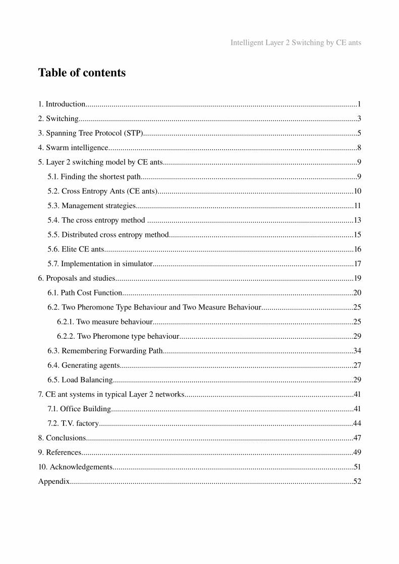
Table of contents
1. Introduction.......................................................................................................................................1
2. Switching..........................................................................................................................................3
3. Spanning Tree Protocol (STP)..........................................................................................................5
4. Swarm intelligence...........................................................................................................................8
5. Layer 2 switching model by CE ants................................................................................................9
5.1. Finding the shortest path...........................................................................................................9
5.2. Cross Entropy Ants (CE ants).................................................................................................10
5.3. Management strategies............................................................................................................11
5.4. The cross entropy method ......................................................................................................13
5.5. Distributed cross entropy method...........................................................................................15
5.6. Elite CE ants............................................................................................................................16
5.7. Implementation in simulator....................................................................................................17
6. Proposals and studies......................................................................................................................19
6.1. Path Cost Function..................................................................................................................20
6.2. Two Pheromone Type Behaviour and Two Measure Behaviour.............................................25
6.2.1. Two measure behaviour...................................................................................................25
6.2.2. Two Pheromone type behaviour......................................................................................29
6.3. Remembering Forwarding Path..............................................................................................34
6.4. Generating agents....................................................................................................................27
6.5. Load Balancing.......................................................................................................................29
7. CE ant systems in typical Layer 2 networks....................................................................................41
7.1. Office Building........................................................................................................................41
7.2. T.V. factory..............................................................................................................................44
8. Conclusions.....................................................................................................................................47
9. References.......................................................................................................................................49
10. Acknowledgements.......................................................................................................................51
Appendix............................................................................................................................................52
Intelligent Layer 2 Switching by CE ants
1. Introduction
Nowadays, there are millions of computers in the world. The computer's “boom” was in 90's, when
public computer networks started to be accessible to most of the people. Networks are bigger and
bigger every day since they started and they have needed devices (hardware and software) to help
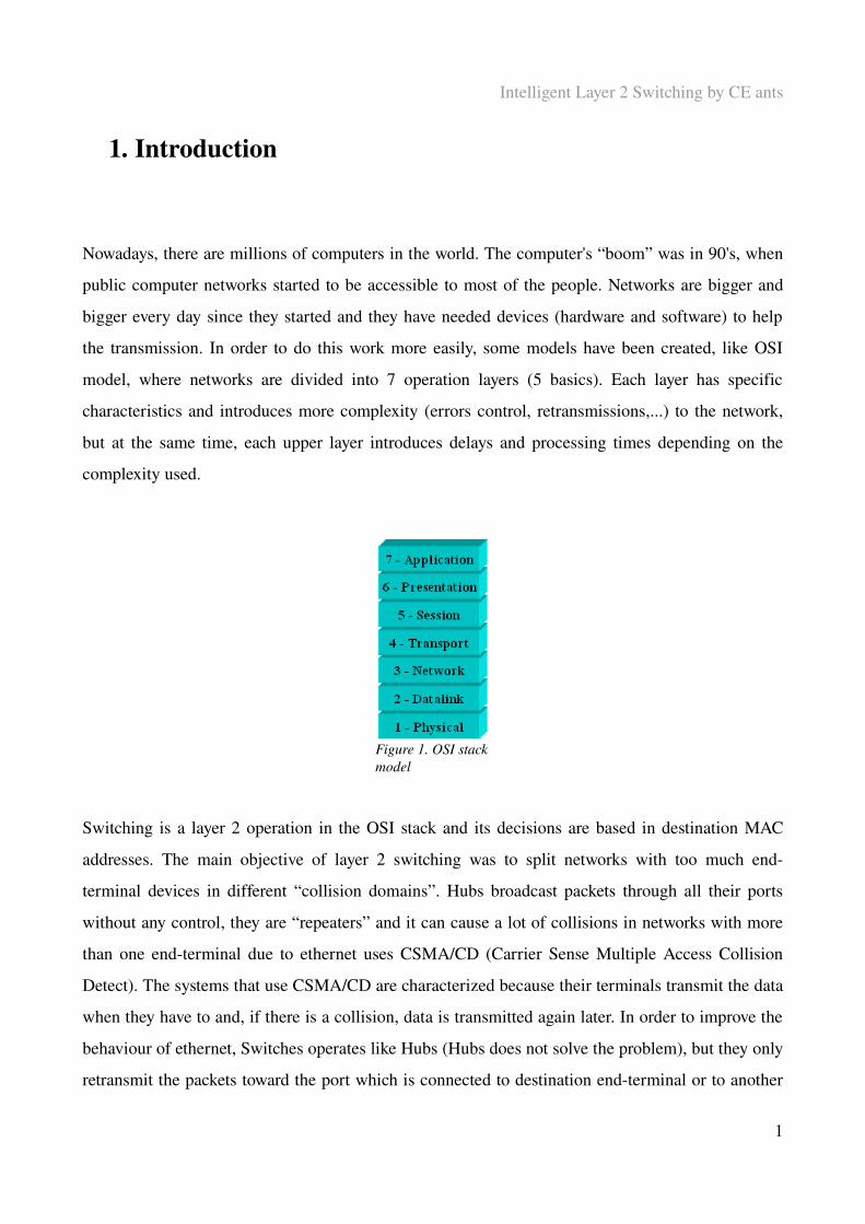
the transmission. In order to do this work more easily, some models have been created, like OSI
model, where networks are divided into 7 operation layers (5 basics). Each layer has specific
characteristics and introduces more complexity (errors control, retransmissions,...) to the network,
but at the same time, each upper layer introduces delays and processing times depending on the
complexity used.
Figure 1. OSI stack model
Switching is a layer 2 operation in the OSI stack and its decisions are based in destination MAC
addresses. The main objective of layer 2 switching was to split networks with too much end
terminal devices in different “collision domains”. Hubs broadcast packets through all their ports
without any control, they are “repeaters” and it can cause a lot of collisions in networks with more
than one endterminal due to ethernet uses CSMA/CD (Carrier Sense Multiple Access Collision
Detect). The systems that use CSMA/CD are characterized because their terminals transmit the data
when they have to and, if there is a collision, data is transmitted again later. In order to improve the
behaviour of ethernet, Switches operates like Hubs (Hubs does not solve the problem), but they only
retransmit the packets toward the port which is connected to destination endterminal or to another
1
Intelligent Layer 2 Switching by CE ants
network device that belongs to the path towards destination (Switch operation is explained in
section 2).
Several techniques have been developed in order to find network paths from source to destination,
but most of them have centralized control and they are not adaptive. Applying swarm intelligence to
find paths in the network we improve these issues and add possibility of multipath to the network,
something that is very advantageous for networks with redundant paths.
In this thesis we have studied the layer 2 switching by CE ants, which means to study the use of
swarm intelligence in layer 2 networks. The objectives are to study CE ant systems, to propose
improvements to make better its implementation in real networks, to compare different proposals, to
decide which are the best options and to check the proposals in typical layer two networks. Some
basic issues of functioning of the network, like cost function, how to balance the load, where to take
decisions and others from CE ants networks, organization of pheromones and where to store the
path in order to do backtracking after calculate the value of the pheromone are studied.
In order to find reliable results, the methodology followed has been divided in three parts. The first
one is a theoretical study proposing solutions to the problems and comparing which advantages and
disadvantages can each option have. For us to know if the proposals work in critical situations in
networks, the second part has been to do simulations and comparing the different proposals with the
results of simulations (they are done with NS2 simulator, modifications over extension by Otto
Wittner, what has spend most time in the making of this thesis), some typical layer 2 networks has
been studied in this part of the work. Finally, the conclusions come from a mix between both
methods (theoretical study and simulation study), reflecting upon the results and deciding which is
the best solution.
2
Intelligent Layer 2 Switching by CE ants
2. Switching
In the introduction the basis of the Layer 2 (and basis of switching) has been explained, and in this
section it is illustrated how the switches (switch devices), whose behaviour belong to Layer 2 in the
OSI stack, work in order to view the behaviour of network units. Therefore, switching is the name
of the behaviour of the networks with switches (or bridges).
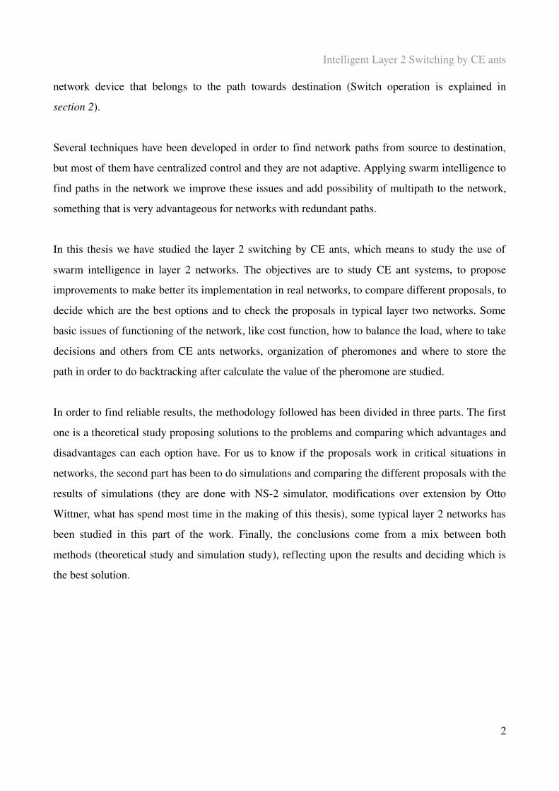
A Switch is a device that can connect different types of packet switched network segments
(Ethernet, Token Ring, Fibre Channel or others) together to form heterogeneous network operating
at OSI layer 2. They are devices that have MAC addresses for each port and are connected to other
devices with MAC addresses, which with these, the switches decide where to send the packets
(frames).
Figure 2. Switch connected to a network and end terminals
Switch operation:
As frame (layer 2 packet) comes into the switch, the incoming port is identified, and port ID is
stored in the switch's MAC addresses table with the originating MAC address. This table often uses
a contentaddressable memory, so it is sometimes called the “CAM table”. Then, the switch
transmits selectively the frame through specific ports decided by comparing the frame's destination
MAC address and previous entries in the MAC addresses table. If destination MAC address is
unknown (it is not in MAC addresses table), the switch transmits the frame out of all ports of the
3
Intelligent Layer 2 Switching by CE ants
connected interfaces except incoming port. If the destination MAC address is known, the frame is
forwarded only to the port related with this destination MAC address in the MAC addresses table. If
the destination MAC address is the same that incoming port, the frame is filtered out and not
forwarded.
Forwarding methods:
There are four forwarding methods that switches can use:
– Cut through: The switch only reads up to the frame's MAC address before starting to forward.
There is no error checking in this method.
– Store and forward: the switch buffers and, typically, performs a checksum on each frame before
forwarding it.
– Fragment free: The switch check first 64 bytes of the frame, where addressing information is
stored. There is no data error checking.
– Adaptive switching: Automatically switching between the other three forwarding methods.
4
Intelligent Layer 2 Switching by CE ants
3. Spanning Tree Protocol (STP)
This thesis talks about special ways to find paths, hence we introduce knowledge about actual
standardized way to find them. The Spanning Tree Protocol (STP) is a method to define different
paths on a network in order to improve some of its issues. It is defined by IEEE in 802.1d1998
Standard (nowadays, the standard working is 802.1d2004, where STP was suppressed and Rapid
STP, RSTP, was included, but both follow the same basis, although there are several proposals in the
“network investigation world” to find optimal paths.)
The Spanning Tree Protocol (STP) disables, with its algorithm, redundant paths in a network to
avoid loops, and enables them when a fault, such as a broken link or node, in the network means
that loops are needed to keep traffic flowing.
LANs and switches can be connected in an arbitrary topology resulting in more than one path
between two switches. If there are loops in the network, frames transmitted onto the network would
circulate around the loop indefinitely, decreasing the performance of the LAN. On the other hand,
multiple paths through the network provide the opportunity for redundancy and backup in network
faults. The Spanning Tree is created through the exchange of Bridge Protocol Data Units (BPDUs)
between the switches in the LAN when they start up, or when a change in the configuration of the
network is detected.
There are many algorithms to “construct” Spanning Trees, they differ in optimization, speed and
load for the construction and special advantages, but all of them ensures that the LAN contains no
loops and that all nodes (or LANs if the spanning tree is been constructed for an extended LAN) are
connected by:
5
Intelligent Layer 2 Switching by CE ants
– Detecting the presence of loops and automatically computing a logical loopfree portion of the
topology, called Spanning Tree.
– Automatically recovering from a switch failure that would split LAN by reconfiguring the
spanning tree to use redundant paths, if available.
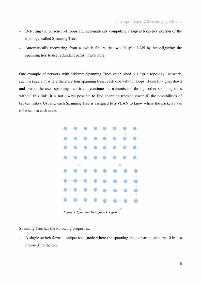
One example of network with different Spanning Trees established is a “grid topology” network,
such in Figure 3, where there are four spanning trees, each one without loops. If one link goes down
and breaks the used spanning tree, it can continue the transmission through other spanning trees
without this link (it is not always possible to find spanning trees to cover all the possibilities of
broken links). Usually, each Spanning Tree is assigned to a VLAN to know where the packets have
to be sent in each node.
Figure 3. Spanning Trees for a 4x4 grid
Spanning Tree has the following properties:
– A single switch forms a unique root (node where the spanning tree construction starts, 0 in last
Figure 3) to the tree.
6
Intelligent Layer 2 Switching by CE ants
– Each switch or LAN in the tree, except the root switch, has a unique parent, known as the
designated switch.
– Each port connecting a switch to a LAN has an associated cost. The root path cost is the sum of
the costs for each segment between the switch and the root switch.
The algorithms uses the following process to establish the spanning tree:
1. A unique root switch is elected by the switches in LAN
2. A designated switch is elected for each LAN in the extended LAN by the switches in the
LAN.
3. The logical spanning tree is computed with an algorithm and redundant paths are removed.
The maintenance of spanning trees is done by replacing a failed path with a redundant backup path,
detecting and removing loops by declaring ports as redundant and removing them from the logical
spanning tree, and maintaining timers that control the ageing of the forwarding database entries.
Spanning Tree Protocol has some advantages and disadvantages, and what we look for with CE ant
systems is how to improve the finding path system and take advantage from disadvantages of STP.
We want a system that find paths without loops and automatically recovers from failures, which are
the advantages of STP, and solve the disadvantages of it, that are to have load dependence,
adaptability to the network changes and support for multipath switching.
7

Intelligent Layer 2 Switching by CE ants
4. Swarm intelligence
Swarm intelligence (SI) is an artificial intelligence technique based around the study of collective
behaviour in decentralized, selforganized systems. Swarm intelligence is a metaphor to solve
distributed problems like animals in nature. Swarm is a group of autonomous animals that are
distributed, but each one is involved in group work without centralized control. Each individual can
communicate with the group through any signal (i.e. pheromones to decide the path to get the food
in ants colonies). In our model, each individual animal will be an agent that will have this
behaviour.
The main characteristics of swarm intelligence systems are:
– Autonomy, human supervision is not needed.
– Adaptability, system changes are detected and the agents can decide new paths in case of
environment changes. The simile in networks would be adding or disconnecting nodes or
failures in the network links.
– Fast propagation of changes through the system.
– Scalability, the population can be increased or reduced.
– There is no central control, so most of the failures in the system can be solved by itself.
– The agents work in parallel, and this means that there are a lot of searching path “threads” at
the same time.
8
Intelligent Layer 2 Switching by CE ants
5. Layer 2 switching model by CE ants
This section is based on a mix of two papers with references [2] and [3], written by Bjarne E.
Helvik, Otto Wittner and Poul Heegaard.
5.1. Finding the sh ortest path
The main issue of all routing systems for networks is to
transmit the data between a given source and destination
by the optimal path (optimal path may mean different
things depending on the design of the network; the path
is optimal in terms of cost, and cost can be defined such
Q2S, delay, free bandwidth, transmission time...) Some
examples are BGP and OSPF in Internet.
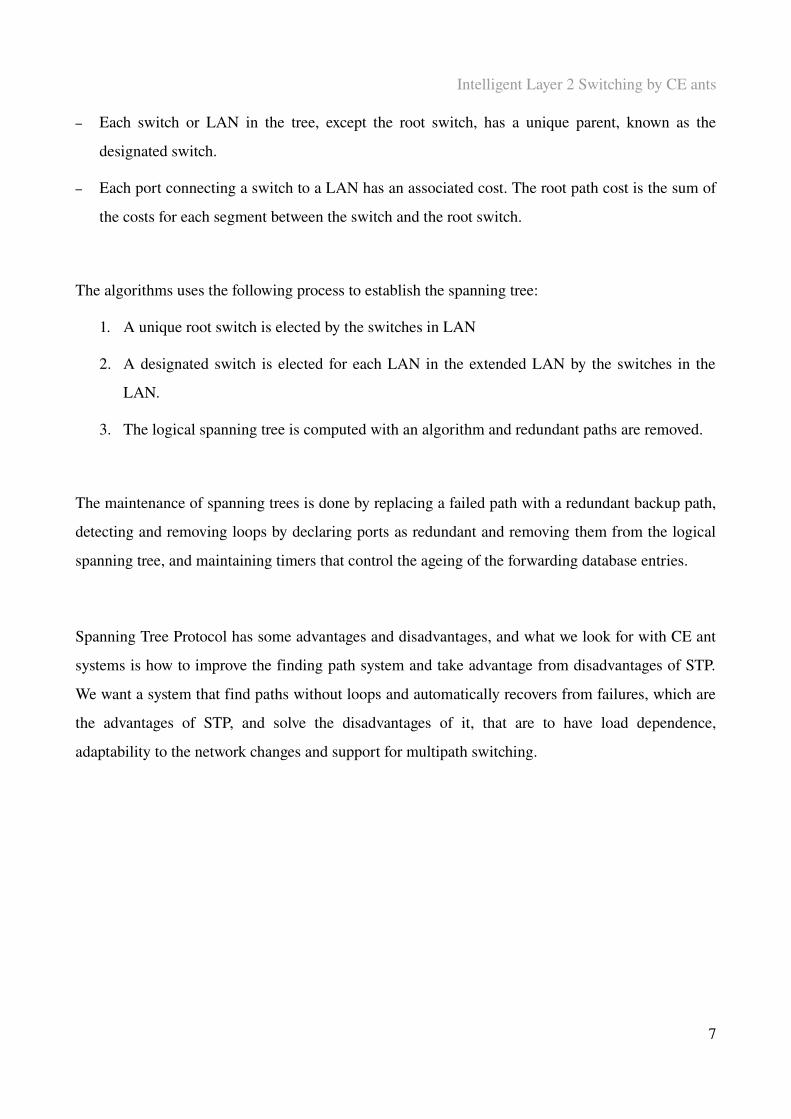
Swarm intelligence systems based on ants finding food
behaviour are able to find a solution close to the optimal
path between a source and destination. Figure 4 shows
how an ant colony changes the path (reroute) when an
obstacle appears. Number 1 in this figure shows the
system “running”, where ants are travelling through the
shortest path, and if an obstacle appears, ants cannot
follow the pheromones (2 in figure) and explore new
paths, in this case two different options, both sides of
the obstacle (number 3) that have the same probability
that the ants go through them. Due to the fact that the
upper path is shorter, ants walking on it will leave more
and stronger pheromones and the next ants will follow
the path with more pheromones (number 4). Number 5
9
Figure 4. Ant colony behaviour when an obstacle is found
Nest Food
Nest Food
Nest Food
Nest Food
Nest Food1
3
24
1)
2)
3)
4)
5)
Pheromone Ant
Intelligent Layer 2 Switching by CE ants
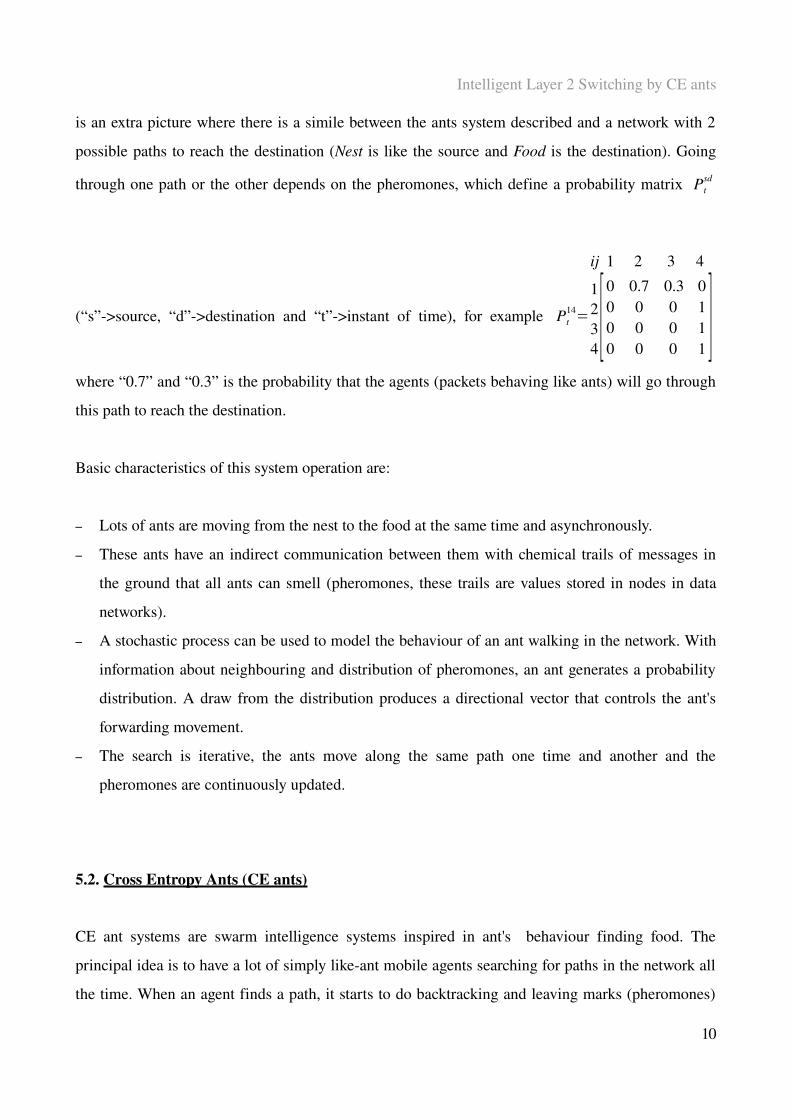
is an extra picture where there is a simile between the ants system described and a network with 2
possible paths to reach the destination (Nest is like the source and Food is the destination). Going
through one path or the other depends on the pheromones, which define a probability matrix Ptsd
(“s”>source, “d”>destination and “t”>instant of time), for example
ij 1 2 3 4
Pt14=
1234[0 0.7 0.3 00 0 0 10 0 0 10 0 0 1
]where “0.7” and “0.3” is the probability that the agents (packets behaving like ants) will go through
this path to reach the destination.
Basic characteristics of this system operation are:
– Lots of ants are moving from the nest to the food at the same time and asynchronously.
– These ants have an indirect communication between them with chemical trails of messages in
the ground that all ants can smell (pheromones, these trails are values stored in nodes in data
networks).
– A stochastic process can be used to model the behaviour of an ant walking in the network. With
information about neighbouring and distribution of pheromones, an ant generates a probability
distribution. A draw from the distribution produces a directional vector that controls the ant's
forwarding movement.
– The search is iterative, the ants move along the same path one time and another and the
pheromones are continuously updated.
5.2. Cross Entropy Ants (CE ants)
CE ant systems are swarm intelligence systems inspired in ant's behaviour finding food. The
principal idea is to have a lot of simply likeant mobile agents searching for paths in the network all
the time. When an agent finds a path, it starts to do backtracking and leaving marks (pheromones)
10

Intelligent Layer 2 Switching by CE ants
like trails left by real ants as it has been expressed before. Due to the quality of the path found, the
pheromones will have more or less strength. Pheromones are stored in network nodes, actually,
nodes hold distributions of pheromones pointing toward their neighbour nodes. When a new agent,
searching destination, arrives to the node, it selects the next node to visit stochastically based on the
pheromone distribution seen in the visited node. Using such ant trail marking, together with the
evaporation of the pheromone, the overall process converges quickly toward having the majority of
the agents following a single trail that tends to be a nearly optimal path. The behaviour of Cross
Entropy ants is, in addition to a copy of the behaviour of real ants, founded in Rubinstein's stochastic
optimization method.
The path management strategy implemented depends on how the quality of the path is determined,
that is how to calculate the cost (cost is the lack of quality). Traffic streams between pairs of nodes
in the network are indexed by m. A path for this stream found by the t’th agent is denoted tm . A
link connecting two adjacent nodes i, j has a link cost Lij . The link cost may depend on the traffic
stream to be carried and when the cost is observed. If this is the case the cost observed by the t’th
ant is denoted L t ,ijm . The cost function, L , of a path is the sum of the link costs, i.e.
Eq. 1
5.3. Management strategies
Management strategy should be reflected in the path cost function of each individual ant to
determine the cost due to wanted behaviour. Two of most important strategies are presented:
– Primary/Backup:
The objective of this strategy is to provide guarantees for maintenance of the service in a single
link failure. This is done finding pairs of disjoint paths, primary and backup. For this reason,
ants searching primary paths should detest ants searching backup paths. The capacity of the
11
L tm=∑
ij∈tm
L t , ijm
Intelligent Layer 2 Switching by CE ants
primary paths will be used in fault free operation, and ants finding primary paths should detest
each other because using a common link could cause overload. On backup paths, the capacity
will be allocated and shared with other backup paths. Backup paths having primary paths with
common links should avoid using common links in the backup path in order to avoid overload in
backup common link if there is a failure in primary common link. All these requests must be
reflected in path cost function, giving high penalties to the paths that do not fulfil them.
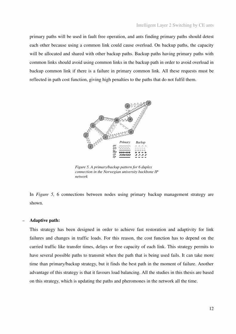
Figure 5. A primary/backup pattern for 6 duplex connection in the Norwegian university backbone IP network
In Figure 5, 6 connections between nodes using primary backup management strategy are
shown.
– Adaptive path:
This strategy has been designed in order to achieve fast restoration and adaptivity for link
failures and changes in traffic loads. For this reason, the cost function has to depend on the
carried traffic like transfer times, delays or free capacity of each link. This strategy permits to
have several possible paths to transmit when the path that is being used fails. It can take more
time than primary/backup strategy, but it finds the best path in the moment of failure. Another
advantage of this strategy is that it favours load balancing. All the studies in this thesis are based
on this strategy, which is updating the paths and pheromones in the network all the time.
12
Intelligent Layer 2 Switching by CE ants
5.4. The cross entropy method
The Cross Entropy method is used to find the optimal solution to discrete combinatorial problems
that are solved based on a KullbackLeibler cross entropy, importance sampling, Markov chain and
the Boltzmann distribution. Next, the method is outlined.
This method, presented by Rubinstein, is based on a random search for an optimal path, even though
there is a very low probability for a path to be optimal (there are a big number of possible paths in a
network, this number increases with the size of the network). Hence, the probability of observing
the optimal path is increased by applying importancesamplinglike technique. In our context, this
approach may be regarded as a centralised search for a single best path in a network. In this section,
the cross entropy (CE) method is summarized with the above “ant terminology” with the
modification that t is now interpreted as a batch of N ants rather than a single ant (it is shown in step
2 of the iteration steps in next paragraph).
The total allocation of pheromones in a network is represented by probability matrix Pt where an
element Pt,ij reflects the normalized intensity of pheromones pointing from node i toward node j. An
ant's stochastic search for a simple path resembles a Markov Chain selection process based on Pt.
By importance sampling in multiple iterations Rubinstein alters the transition matrix (Pt >Pt+1) and
increases, as mentioned, certain probabilities such that agents eventually find nearly optimal paths
with high probabilities. Cross entropy is applied to ensure efficient alternation of the matrix. To
speed up the process even more, a performance function weights the path qualities such that high
quality paths have greater influence on the alternation of the matrix, (in step 2). Rubinstein's CE
algorithm has 4 steps. The indexes m and r are omitted since a single path and single kind of agent
are considered:
1. At the first iteration t = 0, select a start transition matrix Pt=0 (for example, uniformly
distributed)
2. Generate N paths from Pt. Calculate the minimum parameter t , denoted temperature, to
fulfil average path performance constraints, i.e.
13
Intelligent Layer 2 Switching by CE ants
Eq. 2
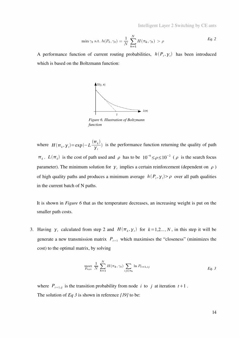
A performance function of current routing probabilities, h Pt ,t has been introduced
which is based on the Boltzmann function:
Figure 6. Illustration of Boltzmann function
where H k ,t=exp −Lk
t is the performance function returning the quality of path
k . L k is the cost of path used and has to be 10−6≤≤10−2 ( is the search focus
parameter). The minimum solution for t implies a certain reinforcement (dependent on )
of high quality paths and produces a minimum average h Pt ,t over all path qualities
in the current batch of N paths.
It is shown in Figure 6 that as the temperature decreases, an increasing weight is put on the
smaller path costs.
3. Having t calculated from step 2 and H k ,t for k=1,2... , N , in this step it will be
generate a new transmission matrix Pt1 which maximises the “closeness” (minimizes the
cost) to the optimal matrix, by solving
Eq. 3
where Pt1, ij is the transition probability from node i to j at iteration t1 .
The solution of Eq 3 is shown in reference [19] to be:
14
Intelligent Layer 2 Switching by CE ants
Eq. 4
where I X =1 if X=true and I X =0 if X= false . Eq 4 become a minimised cross
entropy between Pt and Pt1 , and ensures an optimal shift in probabilities with respect to
t and the performance function.
4. Steps 2 and 3 have to be repeated until H ,≈H ,t1 where is the best path
found.
5.5. Distributed cross entropy method
What today is known as CE ants is a distributed and asynchronous version of Rubinstein's CE
algorithm, developed in reference [20]. By a few approximations, Eq 4 and Eq 2 may be replaced
by autoregressive counterparts based on
Eq. 5
and
Eq. 6
where
Eq. 7
and where ∈⟨0,1⟩ (typically close to 1) controls the history of paths remembered by the system
(i.e. replaces N in step 2). All development of the autoregression is shown in reference [20]. Step
2 and 3 in the algorithm can now be performed immediately after a single new path t is found (t
15
min t s.t. h t ' t
Intelligent Layer 2 Switching by CE ants
again represents the t'th ant), and a new probability matrix Pt1 can be generated. Hence CE ants
may be understood as an algorithm where search ants evaluate a path found (and calculate t by Eq
6) right after they reach their destination node, and then immediately return to their source node
backtracking along the path. During backtracking, pheromones are placed by updating the relevant
probabilities in the transition matrix, i.e. applying H t ,t through Eq 5.
The autoregressive schemas applied in CE ant system are compact, this means that the system
becomes both computationally efficient, requires limited amounts of memory and is simple to
implement.
5.6. Elite CE ants
The concept of elitism in CE ant systems is introduced in reference [18]. The new system, called
elite CE ants, performs significantly better in terms of the number on path traversals required to
converge toward a near optimal path. The kind of distribution an ant makes depends on the cost of
the path it has traversed relative to the cost of the paths found by other ants. All ants contribute in
updating the temperature t as in Eq 6. However, a limited set of ants, denoted the elite set, updates
a different temperature t∗ . Only ants belonging to the elite set backtrack their paths and update
pheromones applying H k ,t∗ in Eq 5, and hence, reducing the total number of backtracking
traversals and pheromone updates.
The criterion for determining if an ant is in the elite set is based on the fact that the best solutions in
CE ants method relates to through e−L t / t , as is shown in step 2 of “The cross entropy
method” section. The elite set criteria is a rearrangement of this relationship. An ant is considered
an elite ant if the cost of the path found by the ant satisfies
Eq. 8
where t is the temperature updated by all ants. Hence, when removing parts of the search space
which enables elite ants to find their paths, for example by a link failure in the best path found, the
16
L t −t ln
Intelligent Layer 2 Switching by CE ants
temperature t will increase and allow ants with higher path costs to perform pheromone updates.
Hence dynamic network conditions are handled. Note also that elite criteria does not introduce any
additional parameters. It is selftuning.
5.7. Implementation in simulator
An extension of NS2 (Network Simulator) for CE ant system has been developed by Otto Wittner in
Telematics department of NTNU university. It has been used for simulations about all theoretic
proposals and studies previously done. Everything that will be explained next, is about swarm
extension without the modifications made to simulate the variants defined in this thesis (they will be
explained later and code can be found in Appendix), so basic knowledge about NS2 simulator are
supposed.
The extension of the simulator is programmed in C++, this language is an object oriented
programming language, this means that there are many classes and that the code is divided in them.
However, in Swarm extension there is one main class called swarmrtm where the biggest part of the
behaviour of the system is defined, how an agent moves in the system and what it does in each node.
Next, the actions in the simulations for an agent will be described, which is very similar to explain
how a CE ants system works.
It is important to know beforehand that three types of packets (agents/ants) are defined. Datapacket
ants are the packets that carry the data that has to be transmitted from source node to destination
node. These agents follow the pheromone system in order to go towards destination through the
optimal path, but they do not modify the gamma of the transmission and do not backtrack (they do
not update the pheromones). Normal ants are the agents that have the behaviour explained in
previous sections. They are little packets that look for optimal paths using CE method. They modify
the gamma when they are at destination and, if they are elite ants, they modify elite gamma and
update pheromones in path nodes when they do the backtracking. Finally, Explorer ants travel in the
network with random (uniform p.d.f) decisions in each node when it has to decide the next. Like
17
Intelligent Layer 2 Switching by CE ants
Normal ants, Explorer ants modify the gamma and they can belong to the elite set. Usually, they
find worst paths than Normal and Datapacket ants, but their use is to observe the network constantly
and if, for example, a new path is added and it is better than the path used by Normal and
Datapacket ants, Explorer ants will find it (more or less quickly depending on the size of the
network and the rate of Explorer ants; as bigger the network and as lower the rate, less probabilities
for a single agent to find that path). When a simulation starts, during the initialization time (set in
TCL script) all the agents have Explorer ants behaviour in order to check all possible paths to decide
which is the optimal one, if this is not done there is a high chance to forget several paths to check,
and maybe they are better (in terms of cost) and unused. Usually, the rate of this packets is much
lower than Normal ants.
When an agent arrives to a node, it checks if the node is a destination node. If the agent (not
Explorer ant, Explorer ants decide their path randomly) is not at destination, it reads which is the
neighbourhood and, for unvisited neighbours, the agent looks at the pheromone vector (where the
pheromone value for each neighbour is stored to reach the destination). If there is no unvisited
neighbours, then the simulator allows to revisit any network (or go home node if home node is
neighbour). With this, the simulator covers all the cases (if there is no pheromones, the decision is
probabilistic with uniform p.d.f.) and an agent can decide which is the next link to go. Two other
things done in each node are to store the node id in the packet, in order to remember the path, and to
calculate the cost of the following link storing it in a field in the agent packet. In the destination
node, agents are differentiated between Datapacket ants and other ants. Datapacket ants are
eliminated (transport of data following pheromones has already been simulated) and Normal and
Explorer ants prepare the backtracking, which means to modify the gamma, to check if the ant is
elite ant or not, and to modify the elite gamma. The ants that do not belong to the elite set are
deleted after modifying the gamma (the behaviour has already been simulated). Elite ants are going
to do the backtracking. Backtracking is to “rewalk” the path from the source to destination but in
reverse direction and updating the pheromone levels for all the nodes where the ant goes and
deleting the node id of the nodes already visited from the agent packet. When the ant returns to the
home node, the packet is deleted (the behaviour has already been simulated).
This is an overview of how the simulator works. Remember that, in Appendix, the modifications to
simulate specific behaviours of this thesis are explained and the code is shown.
18

Intelligent Layer 2 Switching by CE ants
6. Proposals and studies
CE ant systems have been developed theoretically and mathematically and have been simulated in
different systems. What is presented in this section are 4 discussions about proposals of changes to
improve the CE ant systems when they are implemented in a real Layer 2 network and 1 study about
how load balancing works in the system. All these ideas are discussed theoretically first and
simulated later in order to evaluate if it is an improvement or simply a way to discard.
In order to check how the proposals works, a network has been designed with simplicity in order to
be able to easily predict what will happen. This asymmetrical network has few, but sufficient, paths
to make possible its study. These requests are collected in the next network.
network 1. Sample little network that permits the easiness of know when, where and how the things happen
19
Intelligent Layer 2 Switching by CE ants
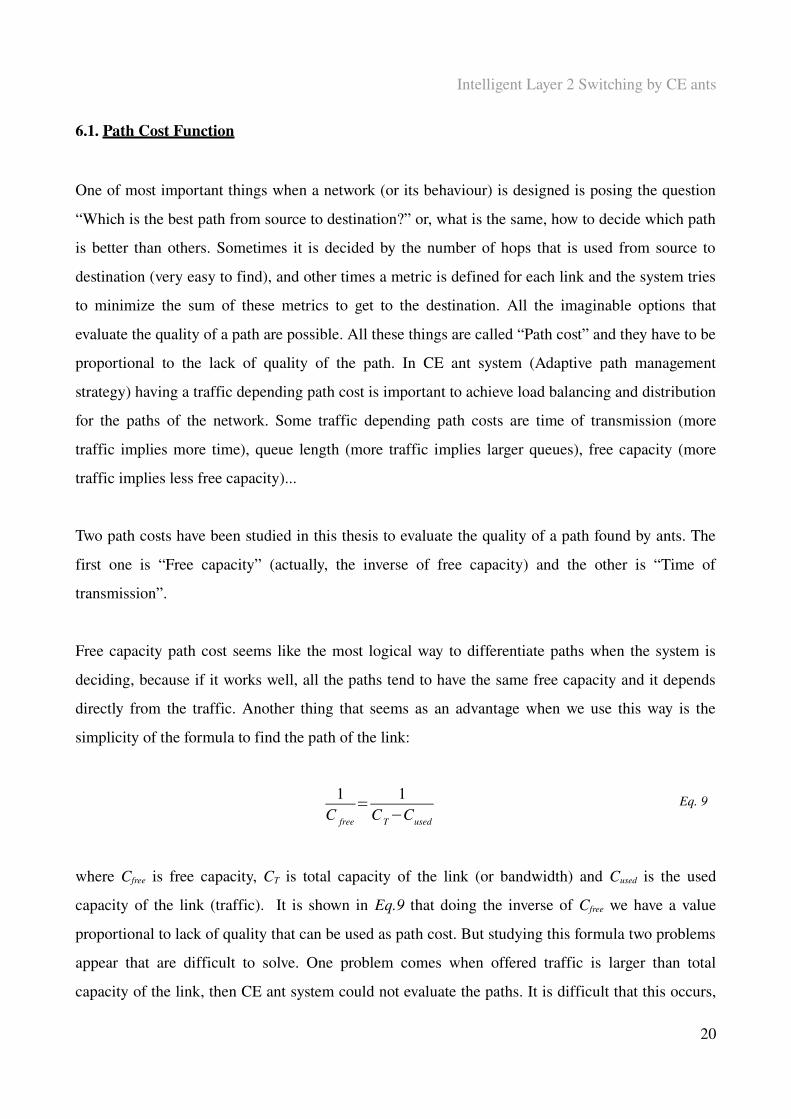
6.1. Path Cost Function
One of most important things when a network (or its behaviour) is designed is posing the question
“Which is the best path from source to destination?” or, what is the same, how to decide which path
is better than others. Sometimes it is decided by the number of hops that is used from source to
destination (very easy to find), and other times a metric is defined for each link and the system tries
to minimize the sum of these metrics to get to the destination. All the imaginable options that
evaluate the quality of a path are possible. All these things are called “Path cost” and they have to be
proportional to the lack of quality of the path. In CE ant system (Adaptive path management
strategy) having a traffic depending path cost is important to achieve load balancing and distribution
for the paths of the network. Some traffic depending path costs are time of transmission (more
traffic implies more time), queue length (more traffic implies larger queues), free capacity (more
traffic implies less free capacity)...
Two path costs have been studied in this thesis to evaluate the quality of a path found by ants. The
first one is “Free capacity” (actually, the inverse of free capacity) and the other is “Time of
transmission”.
Free capacity path cost seems like the most logical way to differentiate paths when the system is
deciding, because if it works well, all the paths tend to have the same free capacity and it depends
directly from the traffic. Another thing that seems as an advantage when we use this way is the
simplicity of the formula to find the path of the link:
Eq. 9
where Cfree is free capacity, CT is total capacity of the link (or bandwidth) and Cused is the used
capacity of the link (traffic). It is shown in Eq.9 that doing the inverse of Cfree we have a value
proportional to lack of quality that can be used as path cost. But studying this formula two problems
appear that are difficult to solve. One problem comes when offered traffic is larger than total
capacity of the link, then CE ant system could not evaluate the paths. It is difficult that this occurs,
20
1C free
=1
CT−Cused

Intelligent Layer 2 Switching by CE ants
but if it happens, the system could crash, because gamma is not prepared to control that. The other
problem is that free capacity of a path should be calculated finding bottle necks and this, as well as
difficult to implement, is useless in ant system, where it is essential that the cost of the path is the
sum of cost of each hop. The next picture shows this problem, where bottle neck of path 1 (nodes 0
135) is 3 and its cost is lower than the cost of path 2 (nodes 0245), as is shown in Eq. 10 and
Eq. 11, whose bottle neck is 5.
network 2. Network to show the problem of bottle necks using CE ant system
Eq. 10
Eq. 11
Time of transmission path cost is the other option studied in this thesis. It is related with the traffic
too, because depending on the traffic on a link, the time of transmission will be higher or lower. The
biggest advantage of this path cost, as well as it is traffic depending, is that the cost is additive, so it
fulfils the requests of CE ant system path cost.
The development to get the formula used to find path cost is:
Eq. 12
21
L 0−1−3−5=∑1
C free
=19
13
19=0,56
L 0−2−4−5=∑1
C free
=15
15
15=0,6
T W=
1−T S
Intelligent Layer 2 Switching by CE ants
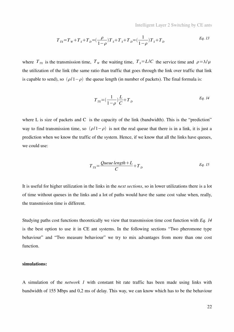
T TX=T WT ST D=
1−T ST ST D=
11−
T ST D Eq. 13
where T TX is the transmission time, T W the waiting time, T S=L /C the service time and =/
the utilization of the link (the same ratio than traffic that goes through the link over traffic that link
is capable to send), so /1− the queue length (in number of packets). The final formula is:
Eq. 14
where L is size of packets and C is the capacity of the link (bandwidth). This is the “prediction”
way to find transmission time, so /1− is not the real queue that there is in a link, it is just a
prediction when we know the traffic of the system. Hence, if we know that all the links have queues,
we could use:
Eq. 15
It is useful for higher utilization in the links in the next sections, so in lower utilizations there is a lot
of time without queues in the links and a lot of paths would have the same cost value when, really,
the transmission time is different.
Studying paths cost functions theoretically we view that transmission time cost function with Eq. 14
is the best option to use it in CE ant systems. In the following sections “Two pheromone type
behaviour” and “Two measure behaviour” we try to mix advantages from more than one cost
function.
simulations:
A simulation of the network 1 with constant bit rate traffic has been made using links with
bandwidth of 155 Mbps and 0,2 ms of delay. This way, we can know which has to be the behaviour
22
T TX=1
1−
LCT D
T TX=Queue lengthL
CT D

Intelligent Layer 2 Switching by CE ants
in each moment. At second 90 of simulation, link between nodes 2 and 5 goes down and it goes up
at second 150.
Figure 7. Transmission time cost graph from a simulation in network 1
Figure 8. Transmission time cost average from a simulation in network 1
As Figure 7 shows, the cost of agents (each point represents one agent) is concentrated around some
lines of cost, these lines are the cost of different possible paths. Most agents are concentrated in
lower cost paths (path decided as better is 0256), as it is logical due to the fact that the CE ant
system behaviour always searches the optimal path. Most of the agents in higher cost paths are
Explorer ants that do not follow pheromones. It is easy to view that between seconds 90 and 150
(while the link between nodes 2 and 5 is down) there is no points in some lines because these lines
are cost lines of paths including a link that is down and ants have to change their path to another
which is up (in this case there are more than one path with the lower cost, they are 01346, 013
56, 02356 and other paths of 4 links). The path decided is 02356 because the utilization is
very low and the load does not have to be distributed between more than one path and this path
decided is the most similar to the path chosen for transmission before the link has gone down. The
most important thing is that ants tend to go through the lowest cost path, and it can be seen in
Average cost graph (Figure 8) which happens while the link is down and the system changes the
path.
23
Intelligent Layer 2 Switching by CE ants
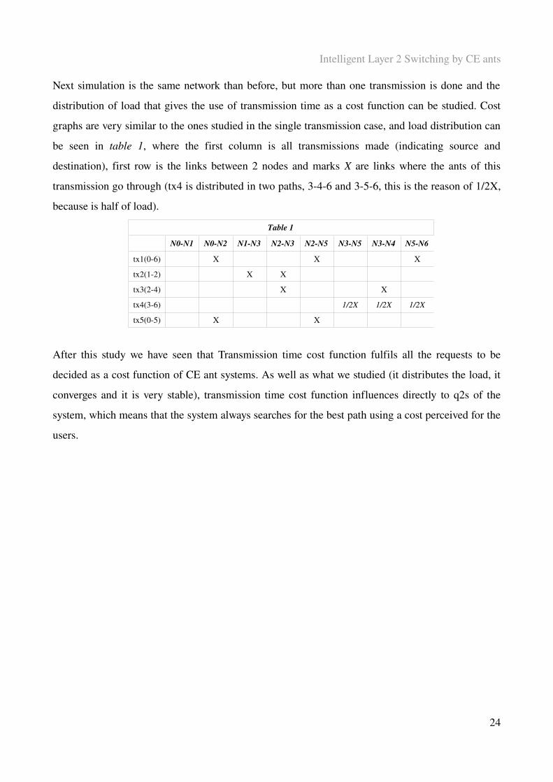
Next simulation is the same network than before, but more than one transmission is done and the
distribution of load that gives the use of transmission time as a cost function can be studied. Cost
graphs are very similar to the ones studied in the single transmission case, and load distribution can
be seen in table 1, where the first column is all transmissions made (indicating source and
destination), first row is the links between 2 nodes and marks X are links where the ants of this
transmission go through (tx4 is distributed in two paths, 346 and 356, this is the reason of 1/2X,
because is half of load).
Table 1
N0N1 N0N2 N1N3 N2N3 N2N5 N3N5 N3N4 N5N6
tx1(06) X X X
tx2(12) X X
tx3(24) X X
tx4(36) 1/2X 1/2X 1/2X
tx5(05) X X
After this study we have seen that Transmission time cost function fulfils all the requests to be
decided as a cost function of CE ant systems. As well as what we studied (it distributes the load, it
converges and it is very stable), transmission time cost function influences directly to q2s of the
system, which means that the system always searches for the best path using a cost perceived for the
users.
24

Intelligent Layer 2 Switching by CE ants
6.2. Two Pheromone Type Behaviour and Two Measure Behaviour
Most cost functions for paths have limits that, when are exceeded, produce wrong cost values or
make the function useless. We can find some examples in cost functions studied in PATH COST
section (section 6.1), where Free capacity cost function does not work in the case that the link
receives more traffic than it can transmit with its bandwidth (it is very rare, but it is possible in
specific moments), or functions for transmission time where, in the case that we use predicted
queues, the system fails in the same case that free capacity and it is far from reality (and not at real
time, it is an average) as higher is the utilization. In transmission time cost function using real
queues, when traffic is close to 0 or very low, it is difficult to differentiate paths using queue
lengths, because most times there are no queues.
In order to solve the problem described, two ideas of modifications for CE ant systems have been
developed, and they are “two pheromone type behaviour” and “two measure behaviour”. Both have
the same idea, to combine two cost functions in one system, but different ways, with different
complexity, different advantages and different disadvantages. Next, they are explained.
6.2.1. Two measure behaviour
Two measure behaviour is a behaviour designed for CE ant systems that combines different cost
functions for each link depending on a condition. In our study case, the condition is the utilization
of the link and different cost functions are the two functions defined in Cost path section for
transmission time (Eq. 14 and Eq. 15). In each node the utilization of the next link is checked, and if
it is higher than a threshold, then it uses the second cost function (using real queues in the function).
If the utilization is lower than threshold, the cost function used is the first one (expected queues in a
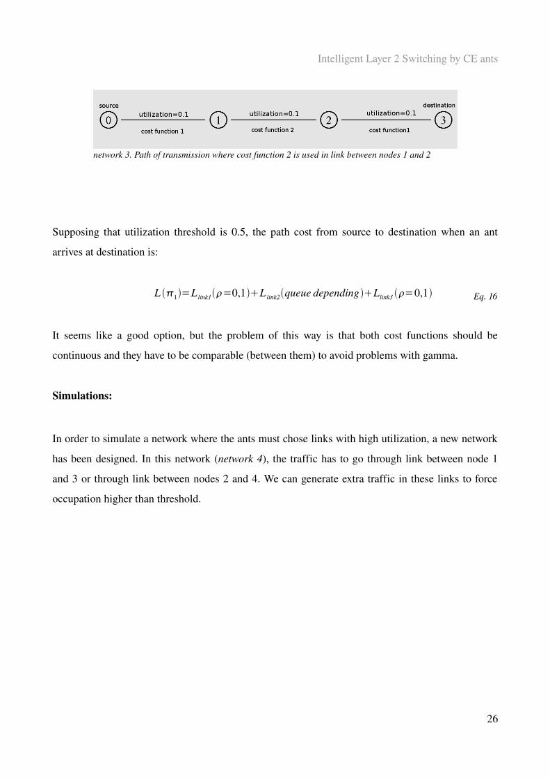
link). Network 3 shows how this proposal works.
25
Intelligent Layer 2 Switching by CE ants
Supposing that utilization threshold is 0.5, the path cost from source to destination when an ant
arrives at destination is:
L 1=L link1=0,1L link2queue depending Llink3 =0,1 Eq. 16
It seems like a good option, but the problem of this way is that both cost functions should be
continuous and they have to be comparable (between them) to avoid problems with gamma.
Simulations:
In order to simulate a network where the ants must chose links with high utilization, a new network
has been designed. In this network (network 4), the traffic has to go through link between node 1
and 3 or through link between nodes 2 and 4. We can generate extra traffic in these links to force
occupation higher than threshold.
26
network 3. Path of transmission where cost function 2 is used in link between nodes 1 and 2
Intelligent Layer 2 Switching by CE ants
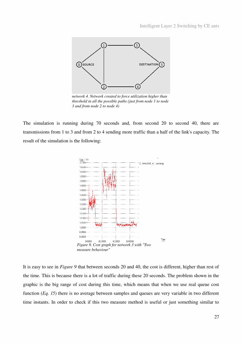
network 4. Network created to force utilization higher than threshold in all the possible paths (just from node 1 to node 3 and from node 2 to node 4)
The simulation is running during 70 seconds and, from second 20 to second 40, there are
transmissions from 1 to 3 and from 2 to 4 sending more traffic than a half of the link's capacity. The
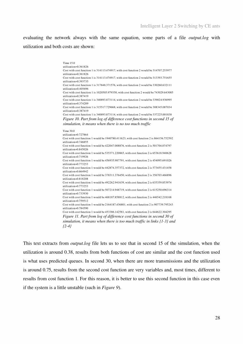
result of the simulation is the following:
Figure 9. Cost graph for network 3 with "Two measure behaviour"
It is easy to see in Figure 9 that between seconds 20 and 40, the cost is different, higher than rest of
the time. This is because there is a lot of traffic during these 20 seconds. The problem shown in the
graphic is the big range of cost during this time, which means that when we use real queue cost
function (Eq. 15) there is no average between samples and queues are very variable in two different
time instants. In order to check if this two measure method is useful or just something similar to
27
Intelligent Layer 2 Switching by CE ants
evaluating the network always with the same equation, some parts of a file output.log with
utilization and both costs are shown:
Figure 10. Part from log of difference cost functions in second 15 of simulation, it means when there is no too much traffic
Figure 11. Part from log of difference cost functions in second 30 of simulation, it means when there is too much traffic in links {13} and {24}
This text extracts from output.log file lets us to see that in second 15 of the simulation, when the
utilization is around 0.38, results from both functions of cost are similar and the cost function used
is what uses predicted queues. In second 30, when there are more transmissions and the utilization
is around 0.75, results from the second cost function are very variables and, most times, different to
results from cost function 1. For this reason, it is better to use this second function in this case even
if the system is a little unstable (such in Figure 9).
28
Time 15.0utilization=0.361826 Cost with cost function 1 is 314113.474917, with cost function 2 would be 314707.253977utilization=0.361826 Cost with cost function 1 is 314113.474917, with cost function 2 would be 313393.751655utilization=0.393735 Cost with cost function 1 is 317848.371576, with cost function 2 would be 330260.632111utilization=0.405696 Cost with cost function 1 is 1020505.979350, with cost function 2 would be 743029.643085utilization=0.387419 Cost with cost function 1 is 340893.873114, with cost function 2 would be 339024.936995utilization=0.374209 Cost with cost function 1 is 315517.729668, with cost function 2 would be 308345.087034utilization=0.387419 Cost with cost function 1 is 340893.873114, with cost function 2 would be 337225.001838
Time 30.0utilization=0.727864 Cost with cost function 1 would be 1940780.411623, with cost function 2 is 864156.752592utilization=0.746855 Cost with cost function 1 would be 422047.008876, with cost function 2 is 501704.074797utilization=0.845026 Cost with cost function 1 would be 535371.220865, with cost function 2 is 653618.940628utilization=0.719926 Cost with cost function 1 would be 456935.987791, with cost function 2 is 454095.691026utilization=0.773253 Cost with cost function 1 would be 442874.357372, with cost function 2 is 573455.431458utilization=0.664942 Cost with cost function 1 would be 378311.376450, with cost function 2 is 356703.466896utilization=0.818208 Cost with cost function 1 would be 492262.941639, with cost function 2 is 635359.853974utilization=0.773253 Cost with cost function 1 would be 507214.948719, with cost function 2 is 615250.696314utilization=0.733930 Cost with cost function 1 would be 468187.858812, with cost function 2 is 446542.218168utilization=0.759512 Cost with cost function 1 would be 2164187.436801, with cost function 2 is 907739.795243utilization=0.784590 Cost with cost function 1 would be 453386.142581, with cost function 2 is 644622.304295
Intelligent Layer 2 Switching by CE ants
6.2.2. Two Pheromone type behaviour
Two pheromone types behaviour is another proposal in the direction to solve the same problem that
two measure behaviour, the problem about the limit of some cost functions and the possibility to use
two different cost functions depending on any parameter. In our case, we have studied both
functions of transmission time cost and the threshold to change the cost function used. The idea of
this behaviour is to have two types of pheromones (it means two pheromone vectors for each node,
two gammas, ..., all duplicated). Usually, just one pheromone type that uses first cost function is
used, but if the threshold (utilization in our case) is exceeded in all possible paths (there is no paths
from source to destination without a link with more occupation than threshold) the system will
change and start to use the other pheromone type, that uses second cost function to calculate the
cost. Theoretically, initialization time where ants search for all the paths is not needed because both
pheromone type agents look for paths with little traffic. It is related with the capacity of links and
the best cost for one pheromone type agents should be the same than for other agents. Instead of
“Two measure behaviour”, in this case, to have similar values from both cost functions is not
necessary because each type of pheromones has its gamma. Next, how the system works is
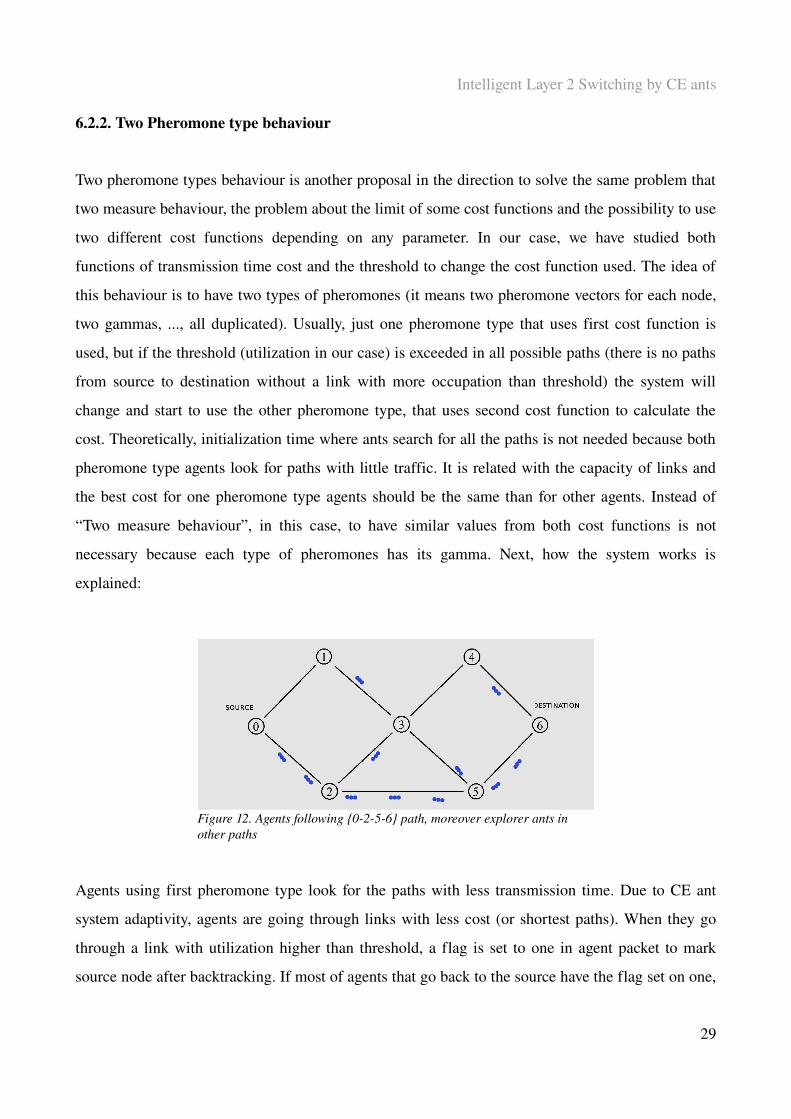
explained:
Figure 12. Agents following {0256} path, moreover explorer ants in other paths
Agents using first pheromone type look for the paths with less transmission time. Due to CE ant
system adaptivity, agents are going through links with less cost (or shortest paths). When they go
through a link with utilization higher than threshold, a flag is set to one in agent packet to mark
source node after backtracking. If most of agents that go back to the source have the flag set on one,
29
Intelligent Layer 2 Switching by CE ants
the system starts to transmit agents using the second pheromone type. One way to control agents
with flag in the source (used in simulator) is to make an average of this bit while agents are arriving
(the size average window can be decided with in Eq. 17) and set a threshold where the used type
of pheromone is changed. The result of make an average is:
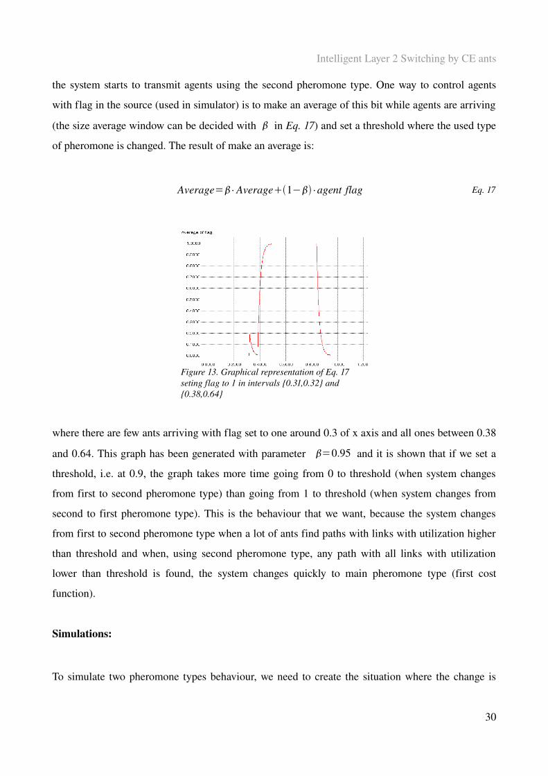
Average=∙ Average1− ∙ agent flag Eq. 17
Figure 13. Graphical representation of Eq. 17 seting flag to 1 in intervals {0.31,0.32} and {0.38,0.64}
where there are few ants arriving with flag set to one around 0.3 of x axis and all ones between 0.38
and 0.64. This graph has been generated with parameter =0.95 and it is shown that if we set a
threshold, i.e. at 0.9, the graph takes more time going from 0 to threshold (when system changes
from first to second pheromone type) than going from 1 to threshold (when system changes from
second to first pheromone type). This is the behaviour that we want, because the system changes
from first to second pheromone type when a lot of ants find paths with links with utilization higher
than threshold and when, using second pheromone type, any path with all links with utilization
lower than threshold is found, the system changes quickly to main pheromone type (first cost
function).
Simulations:
To simulate two pheromone types behaviour, we need to create the situation where the change is
30

Intelligent Layer 2 Switching by CE ants
made, hence, we have used the network 4, where it is easy to create that all paths have at least one
link with more than threshold utilization (the same traffic than Two measure behaviour section
(6.2.1), created between seconds 20 and 40). When we set the threshold of occupation to 0.5 and
threshold of the average for the flag to 0.9, we get the next graphs:
Figure 14. Cost average for a system with Two pheromone type behaviour
Figure 15. Gamma (elite ants + normal ants) for a system with Two pheromone type behaviour
where red lines are the cost and gamma for the agents that follow first pheromone type and green
lines are the cost and gamma for agents that follow second pheromone type. The first problem
observed in both pictures is the adaptivity time taken by the system to go from one pheromone type
to the other one and the unexpected peaks that appear in this moment (change of pheromone types).
Gammas are totally different from each other, something that, as explained before, permits the
system to have cost functions that have different magnitude order. Otherwise, the same problem that
appeared in the “Two measure behaviour” about big range occurs when we use the formula with real
queues (Eq. 15). This problem is easy to solve doing an average (with a small window) of queues,
but doing this average some information is lost and the system stops being updated with real time
information of the network, so we have to be careful with this average and the window that we use.
Looking in simulation output files, we have checked that the load is distributed through paths 024
5 and 0135, assigning less load to the second one, that is the path that has the link whose
bandwidth is 4 Mbps (1 Mbps less than other links in the network).
31

Intelligent Layer 2 Switching by CE ants
In Figure 16 and Figure 17 (zooms from Figure 14), we can see the transitions of cost from the first
pheromone type to the second one and from the second to the first, respectively. What is important
is the pheromone type that has to be used from the given moment, which means that for the
transition between the first and the second pheromone we will study the cost of second pheromone
type and for transition between second and first pheromone type we will study the cost of first
pheromone type. The most important thing to study is the time that it takes to change the method.
First transition time is around 2 seconds, while second transition time is around 1 second. These
times are acceptable compared with the time without using “Two pheromone type behaviour”
(Figure 18 and Figure 19) where time for first transition is around 1.5 seconds and 1 second for
second transition. However, this transition time could be reduced generating some Explorer ants of
the pheromone that does not work.
Figure 16 Moment when system changes from first to second pheromone type
Figure 17. Moment when system changes from first to second pheromone type
32
Intelligent Layer 2 Switching by CE ants
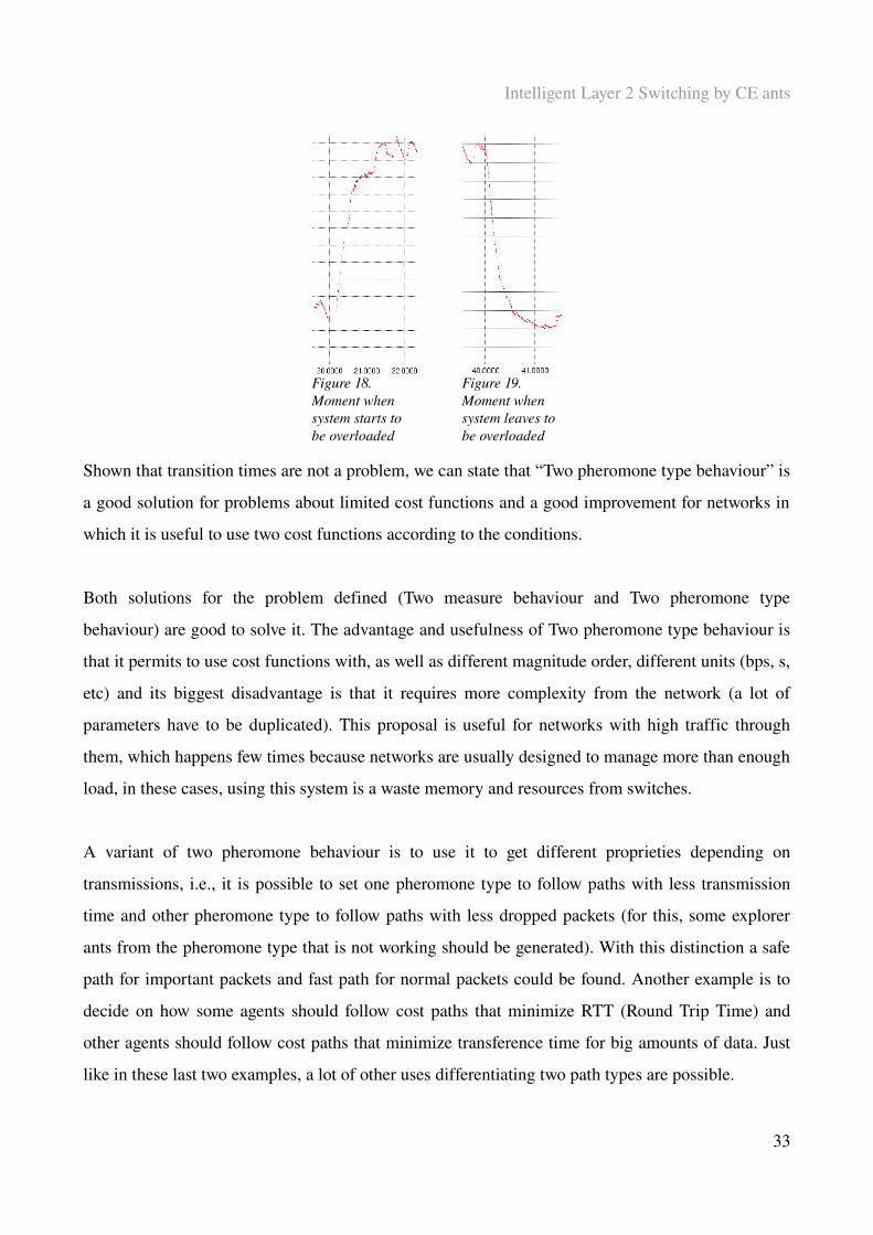
Figure 18. Moment when system starts to be overloaded
Figure 19. Moment when system leaves to be overloaded
Shown that transition times are not a problem, we can state that “Two pheromone type behaviour” is
a good solution for problems about limited cost functions and a good improvement for networks in
which it is useful to use two cost functions according to the conditions.
Both solutions for the problem defined (Two measure behaviour and Two pheromone type
behaviour) are good to solve it. The advantage and usefulness of Two pheromone type behaviour is
that it permits to use cost functions with, as well as different magnitude order, different units (bps, s,
etc) and its biggest disadvantage is that it requires more complexity from the network (a lot of
parameters have to be duplicated). This proposal is useful for networks with high traffic through
them, which happens few times because networks are usually designed to manage more than enough
load, in these cases, using this system is a waste memory and resources from switches.
A variant of two pheromone behaviour is to use it to get different proprieties depending on
transmissions, i.e., it is possible to set one pheromone type to follow paths with less transmission
time and other pheromone type to follow paths with less dropped packets (for this, some explorer
ants from the pheromone type that is not working should be generated). With this distinction a safe
path for important packets and fast path for normal packets could be found. Another example is to
decide on how some agents should follow cost paths that minimize RTT (Round Trip Time) and
other agents should follow cost paths that minimize transference time for big amounts of data. Just
like in these last two examples, a lot of other uses differentiating two path types are possible.
33
Intelligent Layer 2 Switching by CE ants
6.3. Remembering Forwarding Path
Always, when an agent goes through the network, the system has to store the path, in order to
backtrack after the agent finds the destination, and calculate, from cost value obtained along the
path, the pheromones that it will leave in each path node.
One option is to store agent (ant) IDs, agent sources and ingoing ports in tables of each node where
the agent goes through. Agent IDs and agent sources are stored because it is the only possibility to
identify each agent from each node transmitting in CE ant system, and ingoing ports (or previous
nodes) are stored to know where the agent comes from and where it must go after the actual node
during backtracking. Because agents can be dropped or lost and not all the agents do backtracking
(just elite ants), these tables should delete entries for agents that have been more time in the memory
using a timer, thing that is a problem if the network is very large, because then the entries have to be
in the memory a lot of time. The biggest advantage when using this method is that packets do not
have to be modified with any field indicating path. On the other hand, if there are a lot of
transmissions, the tables are bigger and bigger and every time that a packet gets back to the node it
should check this table.
The other option is storing the path followed in ant packet. Each time that an agent arrives to a node,
an identifier for recognition of the path in the backtracking is stored in the packet. This identifier
can be a node ID (size magnitude like MAC addresses, 6 bytes), that stores the path in the agent
packet. By this way it is possible to avoid revisit nodes for each agent and other restrictions that help
agents to find the destination faster. The identifier can also be the ingoing port to the node (Port
IDs), using this identifier, during the backtracking, the node merely has to observe in the packet
which was the ingoing port during forwarding phase and sends the packet toward this port. Using
ingoing port as identifier we lose some advantages like avoiding revisit nodes, but the size of
packets is much lower than using node IDs since most switches have 40 ports as maximum (in
simulations take 256 as maximum to use the worst case, 1 byte needed to store the port ID).
34
Intelligent Layer 2 Switching by CE ants
Simulations:
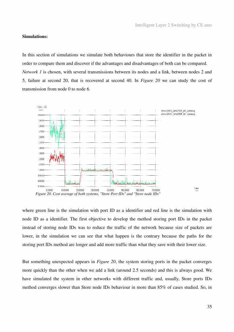
In this section of simulations we simulate both behaviours that store the identifier in the packet in
order to compare them and discover if the advantages and disadvantages of both can be compared.
Network 1 is chosen, with several transmissions between its nodes and a link, between nodes 2 and
5, failure at second 20, that is recovered at second 40. In Figure 20 we can study the cost of
transmission from node 0 to node 6.
Figure 20. Cost average of both systems, "Store Port IDs" and "Store node IDs"
where green line is the simulation with port ID as a identifier and red line is the simulation with
node ID as a identifier. The first objective to develop the method storing port IDs in the packet
instead of storing node IDs was to reduce the traffic of the network because size of packets are
lower, in the simulation we can see that what happen is the contrary because the paths for the
storing port IDs method are longer and add more traffic than what they save with their lower size.
But something unexpected appears in Figure 20, the system storing ports in the packet converges
more quickly than the other when we add a link (around 2.5 seconds) and this is always good. We
have simulated the system in other networks with different traffic and, usually, Store ports IDs
method converges slower than Store node IDs behaviour in more than 85% of cases studied. So, in
35
Intelligent Layer 2 Switching by CE ants
Figure 20, this happens because a small network is used and this specific traffic generated “lucky”
conditions that produce this “illogical” result.
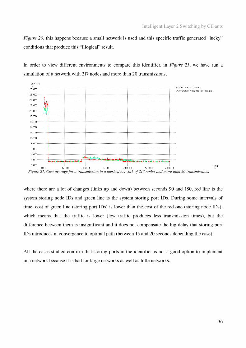
In order to view different environments to compare this identifier, in Figure 21, we have run a
simulation of a network with 217 nodes and more than 20 transmissions,
Figure 21. Cost average for a transmission in a meshed network of 217 nodes and more than 20 transmissions
where there are a lot of changes (links up and down) between seconds 90 and 180, red line is the
system storing node IDs and green line is the system storing port IDs. During some intervals of
time, cost of green line (storing port IDs) is lower than the cost of the red one (storing node IDs),
which means that the traffic is lower (low traffic produces less transmission times), but the
difference between them is insignificant and it does not compensate the big delay that storing port
IDs introduces in convergence to optimal path (between 15 and 20 seconds depending the case).
All the cases studied confirm that storing ports in the identifier is not a good option to implement
in a network because it is bad for large networks as well as little networks.
36

Intelligent Layer 2 Switching by CE ants
6.4. Generating agents
No papers and thesis, this one included, talk about basic and simple things that can affect the system
greatly, such as where to generate agent packets. In order to simulate most characteristics, we use
nodes that generate agent packets and we forget about the possibility that they can be generated in
End Stations (also conversion from cost value to pheromone value and all things told in the thesis
that was made in source and destination nodes could be made in End Stations). There are
differences, advantages and disadvantages summarized in next table:
End Stations
Advantages We can better distribute the traffic if we use CE ant systems only to find the path (i.e. primary backup). One station can be connected to more than one switch and decide which path is better. Switches need less intelligence.
Disadvantages Generates a lot of agent packets (many End Stations are connected to each node usually, so there are more End Stations than nodes in the network). End stations need to work with more intelligence (usually there are more Endstations than switches). It is useless if we have each EndStation connected to one switch because we lose the advantages.
Network Switches
Advantages It reduces the agent packets traffic through the network. It increments the scalability of the network permitting to add End stations and reuse pheromones that have already been put in the system. A EndStation can be added without the need to generate agent traffic. It is easier to simplify the network topology.
DisadvantagesIt is a problem to connect one EndStation to more than one switch. In this situation there would be two different gammas and the system would not know which is the best path from source to destination.
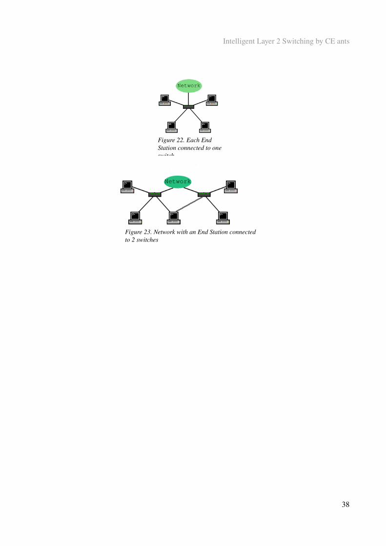
After this Advantages/disadvantages discussion, it is logical to say that using CE ant system
between nodes provides more and better performance in most cases (all cases except when an End
Station is connected to two nodes like in Figure 23, which is very rare in a network).
37
Intelligent Layer 2 Switching by CE ants
Figure 22. Each End Station connected to one switch
Figure 23. Network with an End Station connected to 2 switches
38

Intelligent Layer 2 Switching by CE ants
6.5. Load Balancing
This section is not a proposal or discussion, like last sections, about the system. Instead, this section
is a study of a propriety that can be achieved with CE ant systems (Adaptive management), load
balancing. In other sections (i.e. Path cost section, 6.1) it has been shown that load is distributed in
the network in order to have minimal cost value for all paths. The system is a feedback system, so it
changes depending on previous states:
Figure 24. Scheme for a feedback system
Feedback systems (like Figure 24) change their behaviour depending on their entries and the state of
the system just before these entries. This is the behaviour of CE ant systems, when information is
entered to the system (cost value), it gives an output updating pheromones in the network, output
that is also used to do that new entrance packets (ant packets) arrives to destination through optimal
path.
Load balancing has always been an objective because it minimizes (since network is designed for
more traffic than maximum transmitted) the probability of overload and tries that all paths have the
same cost, or minimum difference between cost of the paths.
As we defined in section Switching by CE ants (section 5) we got for each node, a probability
matrix to decide the next node. Remember Ptsd and Figure 4. With this matrix, the system decides
which ratio of traffic is sent to each node. If two possible paths of the network have the same cost,
the probability matrix will show 0.5 and 0.5 in the positions of these links. If one of them is better
than the other, the system will modify the probabilities until similar proportion between them and
costs is achieved.
39
System
Intelligent Layer 2 Switching by CE ants
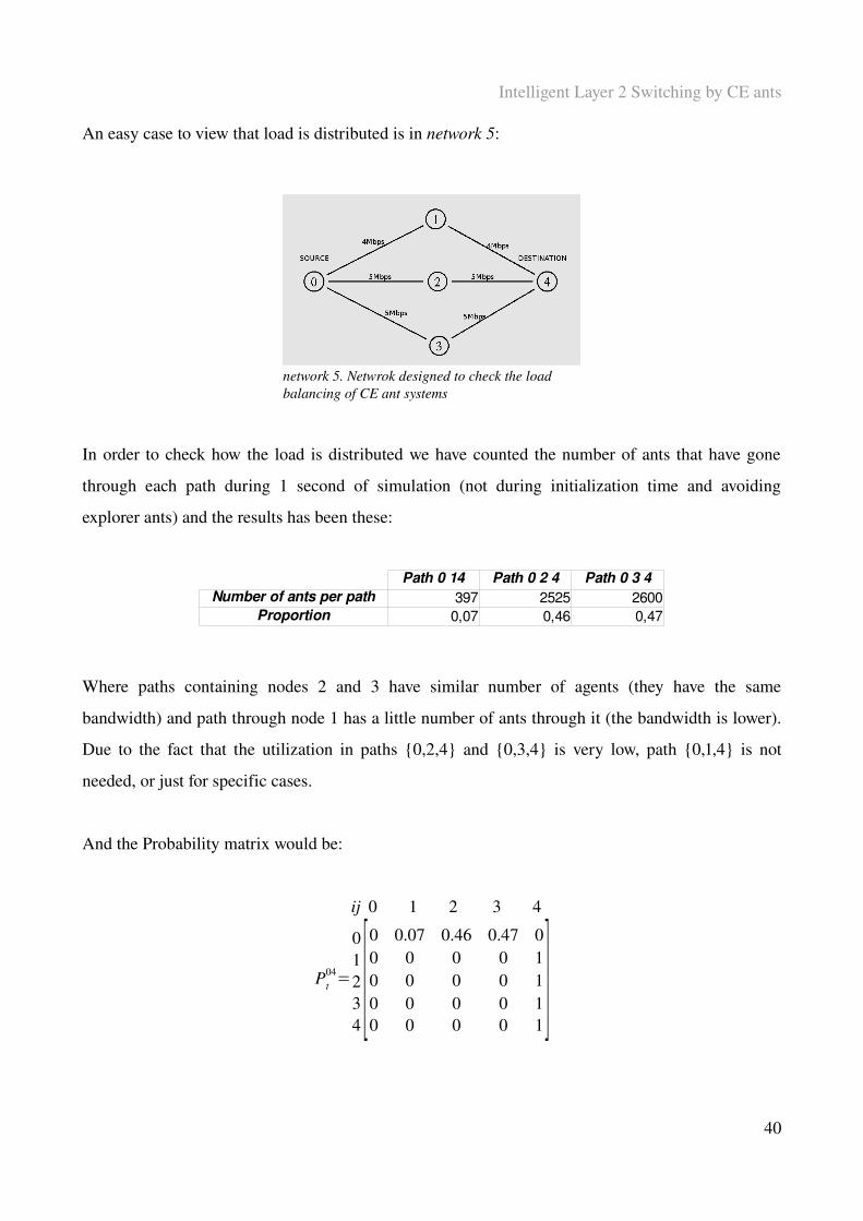
An easy case to view that load is distributed is in network 5:
network 5. Netwrok designed to check the load balancing of CE ant systems
In order to check how the load is distributed we have counted the number of ants that have gone
through each path during 1 second of simulation (not during initialization time and avoiding
explorer ants) and the results has been these:
Path 0 14 Path 0 2 4 Path 0 3 4Number of ants per path 397 2525 2600
Proportion 0,07 0,46 0,47
Where paths containing nodes 2 and 3 have similar number of agents (they have the same
bandwidth) and path through node 1 has a little number of ants through it (the bandwidth is lower).
Due to the fact that the utilization in paths {0,2,4} and {0,3,4} is very low, path {0,1,4} is not
needed, or just for specific cases.
And the Probability matrix would be:
ij 0 1 2 3 4
Pt04=
01234[0 0.07 0.46 0.47 00 0 0 0 10 0 0 0 10 0 0 0 10 0 0 0 1
]40
Intelligent Layer 2 Switching by CE ants
7. CE ant systems in typical Layer 2 networks
In section 6 we have studied different proposals in networks designed specially to view how they
work and check if they are useful in critical situations. In this section we will study typical Layer 2
networks, like an office building and TV factory. It is difficult to study very big networks, so, in
some cases, they have been simplified.
Trondheim's wireless network was a candidate to be studied in this section. We got the topology but
it was a tree topology, so there is just one path from source to destination and CE ant system is
useless. The network was designed a few months ago and it is planned to add redundant paths in the
next months, but the redundant paths added produce a very simple network, similar to cases studied
in proposals and studies section (section 6), so its study has been discarded.
7.1. Office Building
An office building is a place where it is typical to use Layer 2 networks for the internal network and
one router (gateway, Layer 3) to put the traffic to internet.
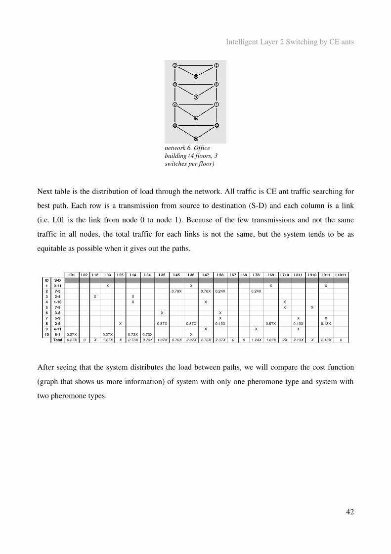
We consider a building of 4 floors (to make the study easier), where 60 people work in each one,
and 3 stairways (network wires go through upstairs holes). In each floor there are three layer 2
switches that are connected between them and have 20 computers connected per switch. Network 6
is which has this topology.
41
Intelligent Layer 2 Switching by CE ants
network 6. Office building (4 floors, 3 switches per floor)
Next table is the distribution of load through the network. All traffic is CE ant traffic searching for
best path. Each row is a transmission from source to destination (SD) and each column is a link
(i.e. L01 is the link from node 0 to node 1). Because of the few transmissions and not the same
traffic in all nodes, the total traffic for each links is not the same, but the system tends to be as
equitable as possible when it gives out the paths.
L01 L02 L12 L03 L25 L14 L34 L35 L45 L36 L47 L58 L67 L68 L78 L69 L710 L811 L910 L911 L1011ID SD1 011 X X X X2 75 0.76X 0.76X 0.24X 0.24X3 24 X X4 110 X X X5 79 X X6 38 X X7 59 X X X8 29 X 0.87X 0.87X 0.13X 0.87X 0.13X 0.13X9 411 X X X
10 61 0.27X 0.27X 0.73X 0.73X XTotal 0.27X 0 X 1.27X X 2.73X 0.73X 1.87X 0.76X 2.87X 2.76X 2.37X 0 0 1.24X 1.87X 2X 2.13X X 2.13X 0
After seeing that the system distributes the load between paths, we will compare the cost function
(graph that shows us more information) of system with only one pheromone type and system with
two pheromone types.
42
Intelligent Layer 2 Switching by CE ants
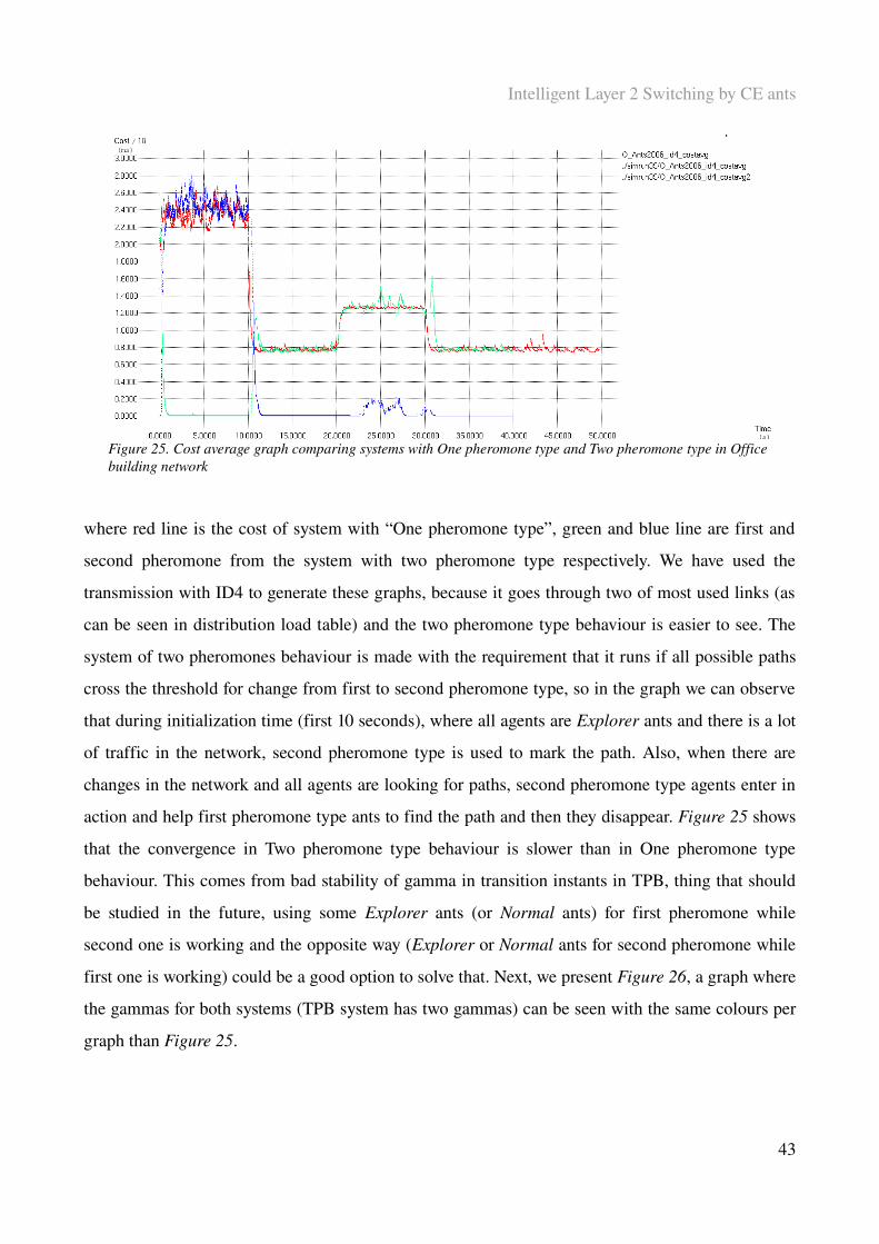
Figure 25. Cost average graph comparing systems with One pheromone type and Two pheromone type in Office building network
where red line is the cost of system with “One pheromone type”, green and blue line are first and
second pheromone from the system with two pheromone type respectively. We have used the
transmission with ID4 to generate these graphs, because it goes through two of most used links (as
can be seen in distribution load table) and the two pheromone type behaviour is easier to see. The
system of two pheromones behaviour is made with the requirement that it runs if all possible paths
cross the threshold for change from first to second pheromone type, so in the graph we can observe
that during initialization time (first 10 seconds), where all agents are Explorer ants and there is a lot
of traffic in the network, second pheromone type is used to mark the path. Also, when there are
changes in the network and all agents are looking for paths, second pheromone type agents enter in
action and help first pheromone type ants to find the path and then they disappear. Figure 25 shows
that the convergence in Two pheromone type behaviour is slower than in One pheromone type
behaviour. This comes from bad stability of gamma in transition instants in TPB, thing that should
be studied in the future, using some Explorer ants (or Normal ants) for first pheromone while
second one is working and the opposite way (Explorer or Normal ants for second pheromone while
first one is working) could be a good option to solve that. Next, we present Figure 26, a graph where
the gammas for both systems (TPB system has two gammas) can be seen with the same colours per
graph than Figure 25.
43
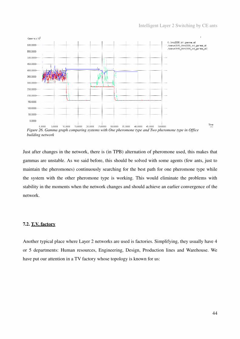
Intelligent Layer 2 Switching by CE ants
Figure 26. Gamma graph comparing systems with One pheromone type and Two pheromone type in Office building network
Just after changes in the network, there is (in TPB) alternation of pheromone used, this makes that
gammas are unstable. As we said before, this should be solved with some agents (few ants, just to
maintain the pheromones) continuously searching for the best path for one pheromone type while
the system with the other pheromone type is working. This would eliminate the problems with
stability in the moments when the network changes and should achieve an earlier convergence of the
network.
7.2. T.V. factory
Another typical place where Layer 2 networks are used is factories. Simplifying, they usually have 4
or 5 departments: Human resources, Engineering, Design, Production lines and Warehouse. We
have put our attention in a TV factory whose topology is known for us:
44
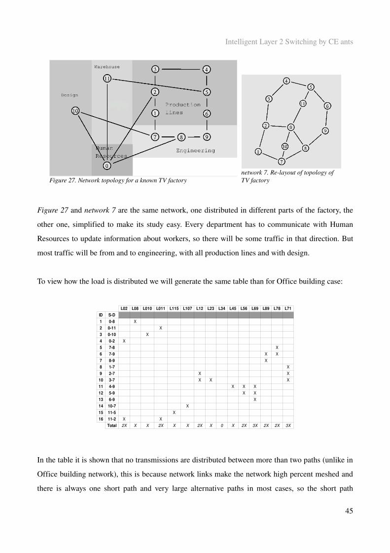
Intelligent Layer 2 Switching by CE ants
Figure 27. Network topology for a known TV factory network 7. Relayout of topology of TV factory
Figure 27 and network 7 are the same network, one distributed in different parts of the factory, the
other one, simplified to make its study easy. Every department has to communicate with Human
Resources to update information about workers, so there will be some traffic in that direction. But
most traffic will be from and to engineering, with all production lines and with design.
To view how the load is distributed we will generate the same table than for Office building case:
L02 L08 L010 L011 L115 L107 L12 L23 L34 L45 L56 L69 L89 L78 L71ID SD1 08 X2 011 X3 010 X4 02 X5 78 X6 79 X X7 89 X8 17 X9 27 X X
10 37 X X X11 49 X X X12 59 X X13 69 X14 107 X15 115 X16 112 X X
Total 2X X X 2X X X 2X X 0 X 2X 3X 2X 2X 3X
In the table it is shown that no transmissions are distributed between more than two paths (unlike in
Office building network), this is because network links make the network high percent meshed and
there is always one short path and very large alternative paths in most cases, so the short path
45
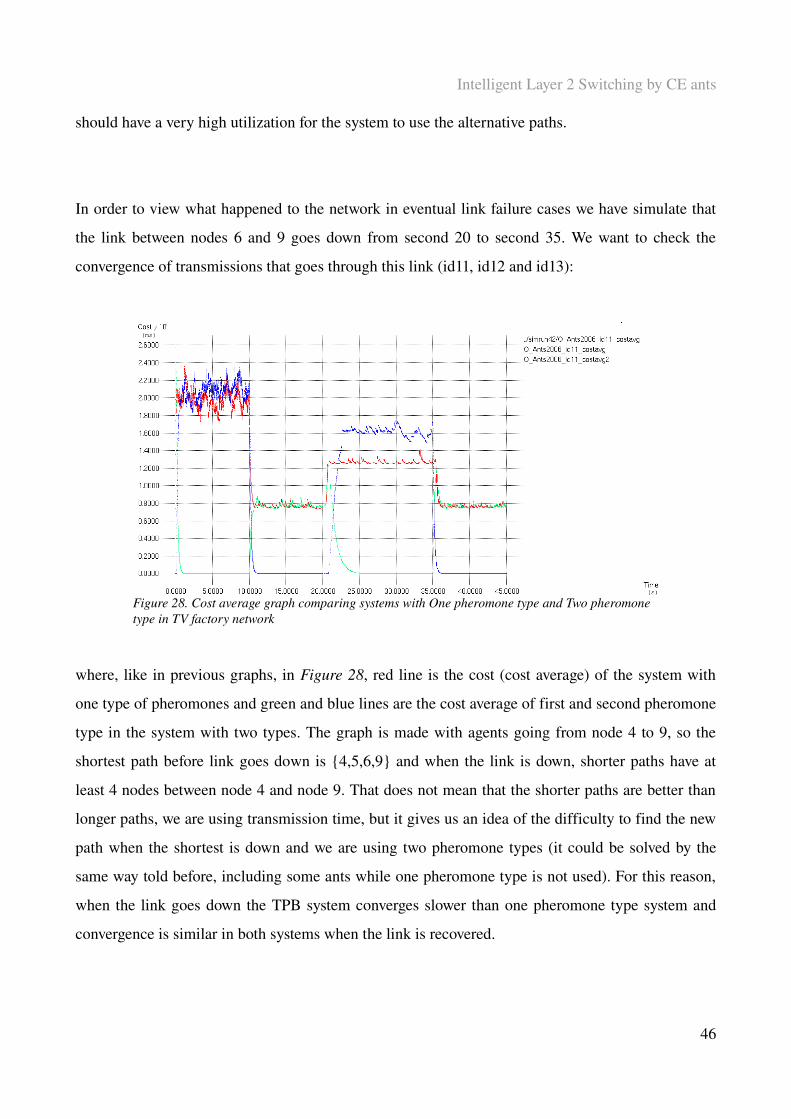
Intelligent Layer 2 Switching by CE ants
should have a very high utilization for the system to use the alternative paths.
In order to view what happened to the network in eventual link failure cases we have simulate that
the link between nodes 6 and 9 goes down from second 20 to second 35. We want to check the
convergence of transmissions that goes through this link (id11, id12 and id13):
Figure 28. Cost average graph comparing systems with One pheromone type and Two pheromone type in TV factory network
where, like in previous graphs, in Figure 28, red line is the cost (cost average) of the system with
one type of pheromones and green and blue lines are the cost average of first and second pheromone
type in the system with two types. The graph is made with agents going from node 4 to 9, so the
shortest path before link goes down is {4,5,6,9} and when the link is down, shorter paths have at
least 4 nodes between node 4 and node 9. That does not mean that the shorter paths are better than
longer paths, we are using transmission time, but it gives us an idea of the difficulty to find the new
path when the shortest is down and we are using two pheromone types (it could be solved by the
same way told before, including some ants while one pheromone type is not used). For this reason,
when the link goes down the TPB system converges slower than one pheromone type system and
convergence is similar in both systems when the link is recovered.
46

Intelligent Layer 2 Switching by CE ants
8. Conclusions
All possible conclusions to be found from the work of this thesis have been discussed in the
subsections of Proposals and Studies (section 6). Hence, conclusions is a summary of all
discussions previously done.
After learning about CE ant systems behaviour, we have proposed 5 ideas to be studied. They are:
– Use of transmission time path cost.
– Use of Two measure behaviour.
– Use of Two pheromone type behaviour.
– Store Port IDs in packets instead of Store node IDs.
– Agent generation in End Stations instead of in Network nodes.
Some of these proposals have been discarded after theoretical study, like where to generate the
agents, we have seen that it introduces disadvantages in face of just one advantage for a very special
case. And other proposals have been discarded after simulations, like in the case of Store port IDs,
which produces the opposite effect desired, and Two measure behaviour, that introduces some
improvements to the system, but worse improvements than Two pheromone type behaviour.
Both transmission time cost and Two pheromone type behaviour have obtained good results in all
our theoretical and simulation tests.
Transmission time cost function fulfils all the requests needed for a CE ant system path cost
function. As well as what we studied (it distributes the load, it converges and it is very stable),
transmission time cost function influence directly to q2s of the system, which means that the system
always searches for the best path using a cost value perceived for the system users.
47
Intelligent Layer 2 Switching by CE ants
Two pheromone type behaviour is also an improvement to the system when we need to use different
cost functions for different environments. In our case, this method improves the system using two
different cost functions depending on the utilization of the links of the path. This behaviour achieves
that for very high utilizations of links we can use a reliable and ontime function and for very low
utilizations, we can use an approximate cost value more useful for our system. The only problem of
TPB systems is the transition moments between the use of two types of pheromones, where, during
little time, there is instability that produces transition times larger than expected.
In the future, the way to improve the TPB should be studied, specifically the problem of transition
times. Our first ideas have been given in this thesis, like generating some ants (Explorer or Normal)
following and updating the pheromone that is not working in the system. Another solution could be
to generate an amount of Explorer ants when a change in the system is detected. Or maybe other
better solutions could be found, but that is the way to follow.
This thesis gives some basic principles and demonstrate that a lot of ideas can be proposed and
studied in the future of CE ant systems, where some of them will be improvements and others just
demonstrations to discard ways of study, but without them, the systems would not be improved.
In the following years, more practical things have to be studied and decided, such as how to design
devices, how to distribute the packets, and other important aspects of the network performance
48

Intelligent Layer 2 Switching by CE ants
9. References
[1] Otto Wittner. Emergent Behavior Based Implements for Distributed Network Management,
2003.
[2] Bjarne E. Helvik and Otto Wittner. Network Resilience by Emergent Behaviour from Simple
Autonomous Agents. NTNU, Trondheim, Norway.
[3] Poul E. Heegaard, Bjarne E. Helvik and Otto Wittner. Selfmanagement of Virtual Paths in
Dynamic Networks. Telenor & NTNU, Norway.
[4] David Allan, Nigel Brag, Alan McGuire, Andy Reid. Ethernet as Carrier Transport
Infrastructure. February 2006, IEEE Communication Magazine.
[5] J. Farkas, C. Antal, G. Toth, L. Westberg. Distributed Resilient Architecture for Ethernet
Networks. October 2005, IEEE Communication Magazine.
[6] Gianni Di Caro, Frederick Ducatelle and Luca Maria Gambardella. AntHocNet: an Ant
Based Hybrid Routing Algorithm for Mobile Ad Hoc Networks. IDSIA, MannoLuggano,
Switzerland.
[7] Otto Wittner, Bjarne E. Helvik and Victor Nicola. Internet Failure Protection using
Hamiltonian pCycles found by Antlike Agents. NTNU, Trondheim, Norway. And University
of Twente, Netherlands.
[8] Poul E. Heegaard and Otto J. Wittner. Selftuned Refresh Rate in a Swarm Intelligence Path
Management System. Telenor and NTNU, Norway.
[9] Poul E. Heegaard, Otto Wittner, Victor F. Nicola and Bjarne Helvik. Distributed
Asynchronous Algorithm for CrossEntropyBased Combinatorial Optimization. Telenor and
NTNU, Norway. And University of Twente, Netherlands.
[10] PieterTjerk de Boer, Dirk P. Kroese, Shie Mannor and Reuven Y. Rubinstein. A Tutorial on
the Cross Entropy Method.
[11] IEEE. IEEE 802.3 – 2005 standard (Ethernet standard).
[12] Mark Fleischer. Foundations of Swarm Intelligence: From Principles to Practice. University
of Maryland, 2003.
49

Intelligent Layer 2 Switching by CE ants
[13] Robert M. Metcalfe and David R. Boggs. Ethernet: Distributed Packet Switching for Local
Computer Networks. Xerox Palo Alto Research Center.
[14] Ethernet Switching Information. http://www.kmj.com/kmjinfo/smenu.html
[15] Sundar Iyer, Amr Awadallah and Nick McKeown. Analysis of a packet switch with
memories running slower than the linerate. Stanford University.
[16] Kennedy Clark and Kevin Hamilton. Cisco LAN Switching.
[17] http://www.utdallas.edu/~jcobb/4390/Spring07/Slides/Switching/switching.pdf. Packet
Switching. The university of Texas at Dallas.
[18] P. E. Heegaard, O. Wittner, V. F. Nicola, and B. E. Helvik, “Distributed asynchronous
algorithm for crossentropybased combinatorial optimization,” in Rare Event Simulation &
Combinatorial Optimization, (Budapest, Hungary), September 78 2004.
[19] R. Y. Rubinstein, “The CrossEntropy Method for Combinatorial and Continuous
Optimization,” Methodology and Computing in Applied Probability, pp. 127–190, 1999.
[20] B. E. Helvik and O. Wittner, “Using the Cross Entropy Method to Guide/Govern Mobile
Agent’s Path Finding in Networks” in Proceedings of 3rd International Workshop on Mobile
Agents for Telecommunication Applications, Springer Verlag, August 1416 2001.
50

Intelligent Layer 2 Switching by CE ants
10. Acknowledgements
I would like to thank my supervisor Bjarne E. Helvik for welcoming and helping me whenever I
have needed it. Moreover, to Otto Wittner for his support understanding NS2 simulator and
friendship during my stay at NTNU. Ideas and advices from both have been decisive to improve this
thesis. Thanks also to Thomas Jelle, for his supply of Trondheim's wireless topology network.
I would also like to thank to my girlfriend, Alba, for her encouragement and patience that have been
crucial for me. I do not forget my brother, Marc, who has made me happy in most heavy moments
during my studies.
Last but not least I would like to thank, for their moral support, to my friends here (Feli, Fonsi,
Rosalia, Luis, Edu, Robert, Gerard, Pablo, Raul, Alejandro, Laura, Berto, Cristina and others),
international students that I have met these 7 last months in Trondheim. I will always remember you.
Thank you for your friendship and make this experience unforgettable. Specially thanks to Gerard
Ferre, who has spend a lot of time correcting the English writing of this thesis.
51
Intelligent Layer 2 Switching by CE ants
Appendix
As we told in section where CE ant system extension for NS2 designed by Otto Wittner, the
programming language is C++ and the code written in C++ is divided by classes. Next, we present
the code of modified files marking which are the modifications made. These files will be supplied
in a CD attached to the thesis. We strongly recommend to study the code from source files, due to
printed is more difficult to understand.
The files that we have modified are (paths from “ns2.30”):
– ~/queue/queue.cc
– ~/queue/queue.h
– ~/link/delay.cc
– ~/link/delay.h
– ~/swarm/common/swarmrtmodule.cc
– ~/swarm/common/swarmrtmodule.h
– ~/swarm/O_Ants2006/O_Ants2006_trace.cc
– ~/swarm/O_Ants2006/O_Ants2006_trace.h
– ~/swarm/O_Ants2006/O_Ants2006_swarmrtm.cc
– ~/swarm/O_Ants2006/O_Ants2006_swarmrtm.h
where O_Ants2006 system is a variant of Ants2006 system designed before.
52
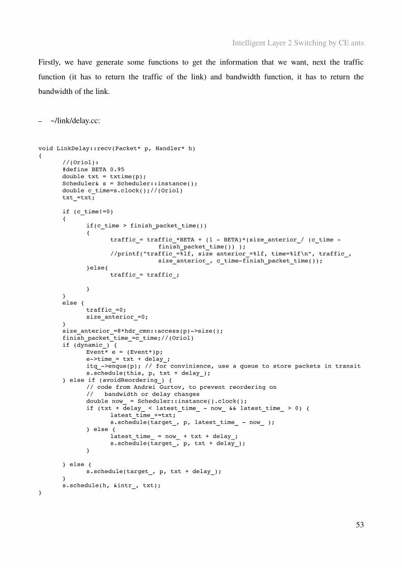
Intelligent Layer 2 Switching by CE ants
Firstly, we have generate some functions to get the information that we want, next the traffic
function (it has to return the traffic of the link) and bandwidth function, it has to return the
bandwidth of the link.
– ~/link/delay.cc:
void LinkDelay::recv(Packet* p, Handler* h){
//(Oriol):#define BETA 0.95double txt = txtime(p);Scheduler& s = Scheduler::instance();double c_time=s.clock();//(Oriol)txt_=txt;
if (c_time!=0) {
if(c_time > finish_packet_time()){
traffic_= traffic_*BETA + (1 BETA)*(size_anterior_/ (c_time finish_packet_time()) );
//printf("traffic_=%lf, size anterior_=%lf, time=%lf\n", traffic_, size_anterior_, c_timefinish_packet_time());
}else{traffic_= traffic_;
}}else {
traffic_=0;size_anterior_=0;
}size_anterior_=8*hdr_cmn::access(p)>size();finish_packet_time_=c_time;//(Oriol)if (dynamic_) {
Event* e = (Event*)p;e>time_= txt + delay_;itq_>enque(p); // for convinience, use a queue to store packets in transits.schedule(this, p, txt + delay_);
} else if (avoidReordering_) {// code from Andrei Gurtov, to prevent reordering on// bandwidth or delay changes
double now_ = Scheduler::instance().clock(); if (txt + delay_ < latest_time_ now_ && latest_time_ > 0) { latest_time_+=txt; s.schedule(target_, p, latest_time_ now_ ); } else { latest_time_ = now_ + txt + delay_; s.schedule(target_, p, txt + delay_); }
} else {s.schedule(target_, p, txt + delay_);
}s.schedule(h, &intr_, txt);
}
53

Intelligent Layer 2 Switching by CE ants
54
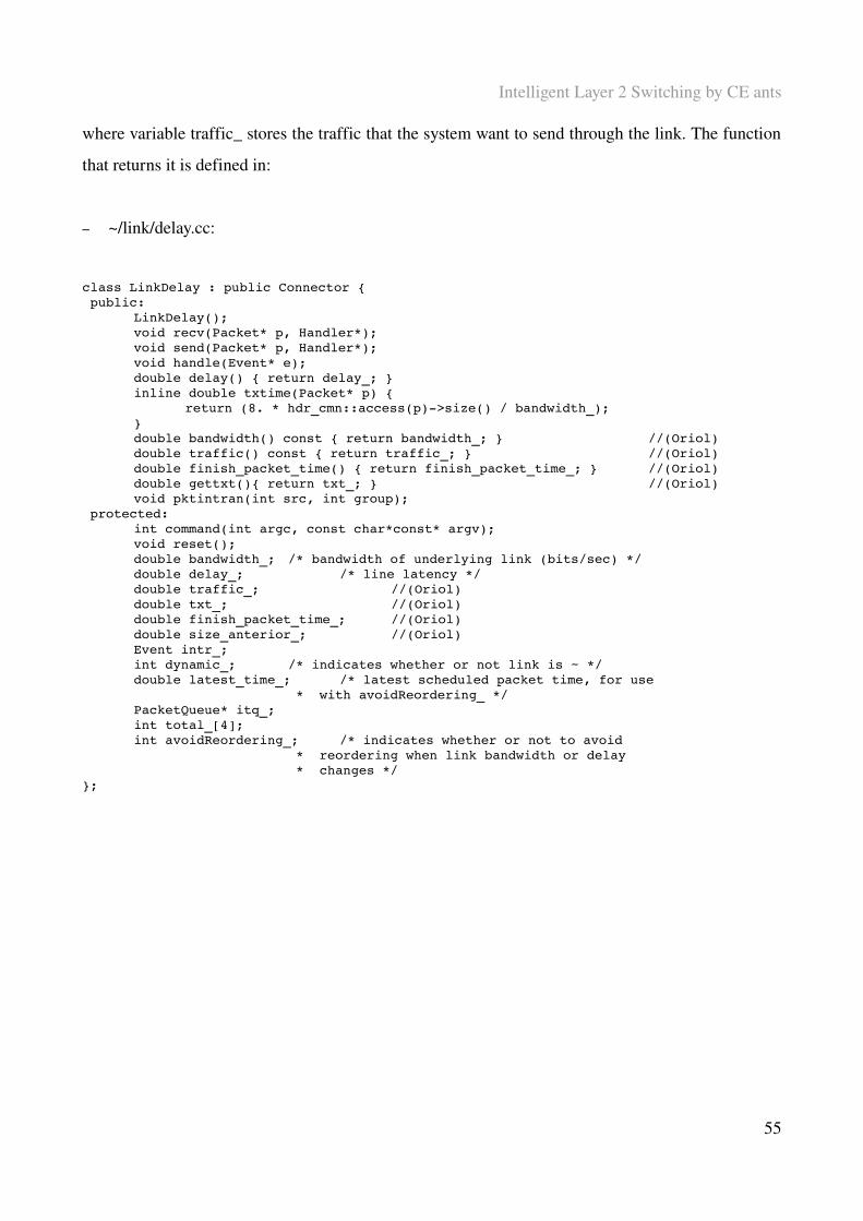
Intelligent Layer 2 Switching by CE ants
where variable traffic_ stores the traffic that the system want to send through the link. The function
that returns it is defined in:
– ~/link/delay.cc:
class LinkDelay : public Connector { public:
LinkDelay();void recv(Packet* p, Handler*);void send(Packet* p, Handler*);void handle(Event* e);double delay() { return delay_; }inline double txtime(Packet* p) {
return (8. * hdr_cmn::access(p)>size() / bandwidth_);}double bandwidth() const { return bandwidth_; } //(Oriol)double traffic() const { return traffic_; } //(Oriol)double finish_packet_time() { return finish_packet_time_; } //(Oriol)double gettxt(){ return txt_; } //(Oriol)void pktintran(int src, int group);
protected:int command(int argc, const char*const* argv);void reset();double bandwidth_; /* bandwidth of underlying link (bits/sec) */double delay_; /* line latency */double traffic_; //(Oriol)double txt_; //(Oriol)double finish_packet_time_; //(Oriol)double size_anterior_; //(Oriol)Event intr_;int dynamic_; /* indicates whether or not link is ~ */double latest_time_; /* latest scheduled packet time, for use
* with avoidReordering_ */PacketQueue* itq_;int total_[4];int avoidReordering_; /* indicates whether or not to avoid
* reordering when link bandwidth or delay * changes */
};
55
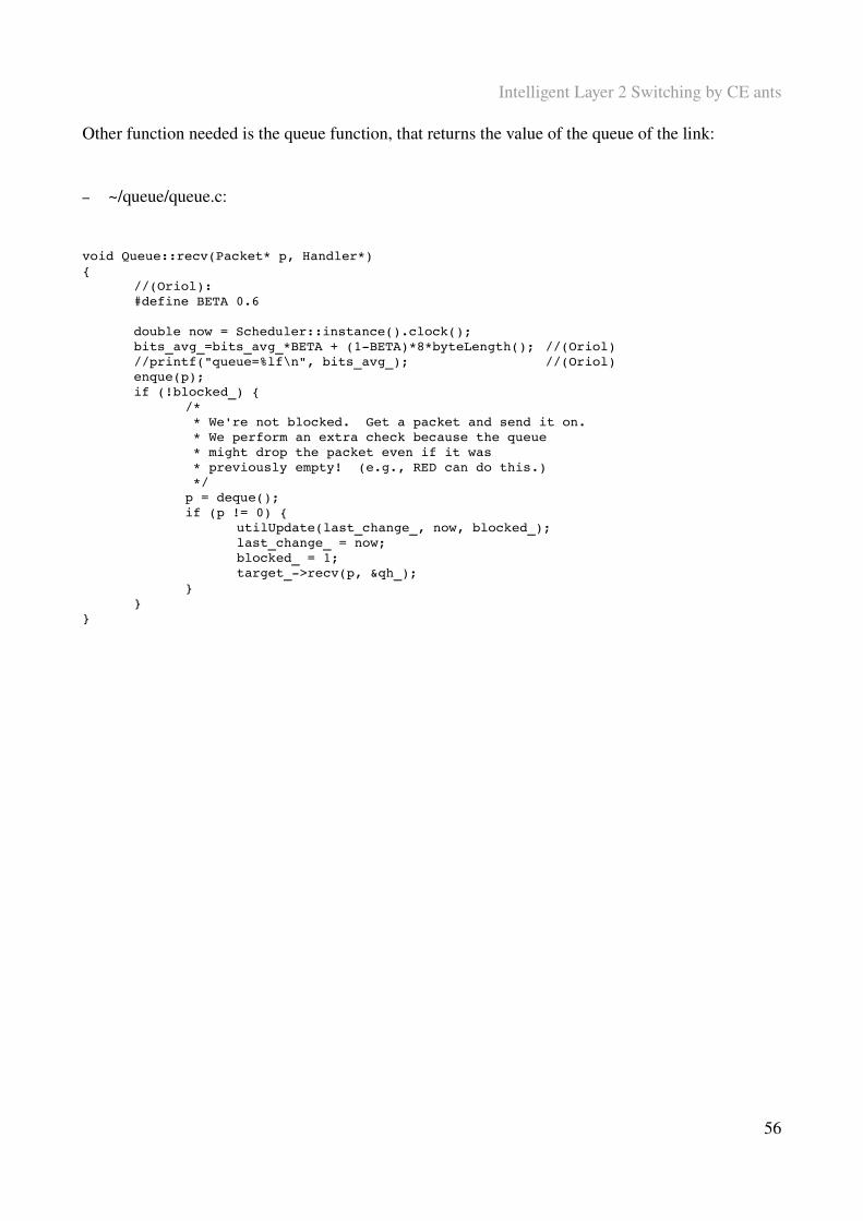
Intelligent Layer 2 Switching by CE ants
Other function needed is the queue function, that returns the value of the queue of the link:
– ~/queue/queue.c:
void Queue::recv(Packet* p, Handler*){
//(Oriol):#define BETA 0.6
double now = Scheduler::instance().clock();bits_avg_=bits_avg_*BETA + (1BETA)*8*byteLength(); //(Oriol)//printf("queue=%lf\n", bits_avg_); //(Oriol)enque(p);if (!blocked_) {
/* * We're not blocked. Get a packet and send it on. * We perform an extra check because the queue * might drop the packet even if it was * previously empty! (e.g., RED can do this.) */p = deque();if (p != 0) {
utilUpdate(last_change_, now, blocked_);last_change_ = now;blocked_ = 1;target_>recv(p, &qh_);
}}
}
56
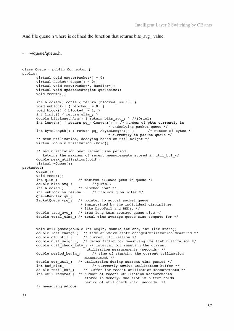
Intelligent Layer 2 Switching by CE ants
And file queue.h where is defined the function that returns bits_avg_ value:
– ~/queue/queue.h:
class Queue : public Connector {public:
virtual void enque(Packet*) = 0;virtual Packet* deque() = 0;virtual void recv(Packet*, Handler*);virtual void updateStats(int queuesize); void resume();
int blocked() const { return (blocked_ == 1); }void unblock() { blocked_ = 0; }void block() { blocked_ = 1; }int limit() { return qlim_; }double bitsLengthAvg() { return bits_avg_; } //(Oriol)int length() { return pq_>length(); } /* number of pkts currently in
* underlying packet queue */int byteLength() { return pq_>byteLength(); } /* number of bytes *
* currently in packet queue *//* mean utilization, decaying based on util_weight */virtual double utilization (void);
/* max utilization over recent time period. Returns the maximum of recent measurements stored in util_buf_*/double peak_utilization(void);virtual ~Queue();
protected:Queue();void reset();int qlim_; /* maximum allowed pkts in queue */double bits_avg_; //(Oriol)int blocked_; /* blocked now? */int unblock_on_resume_; /* unblock q on idle? */QueueHandler qh_;PacketQueue *pq_; /* pointer to actual packet queue
* (maintained by the individual disciplines * like DropTail and RED). */
double true_ave_; /* true longterm average queue size */double total_time_; /* total time average queue size compute for */
void utilUpdate(double int_begin, double int_end, int link_state);double last_change_; /* time at which state changed/utilization measured */double old_util_; /* current utilization */ double util_weight_; /* decay factor for measuring the link utilization */double util_check_intv_; /* interval for reseting the current
utilization measurements (seconds) */double period_begin_; /* time of starting the current utilization
measurement */double cur_util_; /* utilization during current time period */int buf_slot_; /* Currently active utilization buffer */double *util_buf_; /* Buffer for recent utilization measurements */int util_records_; /* Number of recent utilization measurements
stored in memory. One slot in buffer holds period of util_check_intv_ seconds. */
// measuring #drops
};
57

Intelligent Layer 2 Switching by CE ants
58
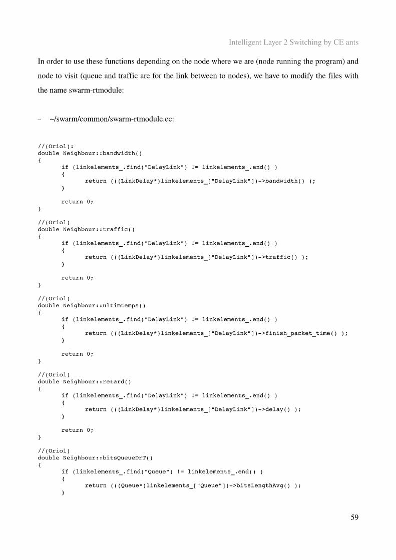
Intelligent Layer 2 Switching by CE ants
In order to use these functions depending on the node where we are (node running the program) and
node to visit (queue and traffic are for the link between to nodes), we have to modify the files with
the name swarmrtmodule:
– ~/swarm/common/swarmrtmodule.cc:
//(Oriol):double Neighbour::bandwidth() {
if (linkelements_.find("DelayLink") != linkelements_.end() ) {
return (((LinkDelay*)linkelements_["DelayLink"])>bandwidth() );}
return 0;}
//(Oriol)double Neighbour::traffic() {
if (linkelements_.find("DelayLink") != linkelements_.end() ) {
return (((LinkDelay*)linkelements_["DelayLink"])>traffic() );}
return 0;}
//(Oriol)double Neighbour::ultimtemps() {
if (linkelements_.find("DelayLink") != linkelements_.end() ) {
return (((LinkDelay*)linkelements_["DelayLink"])>finish_packet_time() );}
return 0;}
//(Oriol)double Neighbour::retard() {
if (linkelements_.find("DelayLink") != linkelements_.end() ) {
return (((LinkDelay*)linkelements_["DelayLink"])>delay() );}
return 0;}
//(Oriol)double Neighbour::bitsQueueDrT() {
if (linkelements_.find("Queue") != linkelements_.end() ) {
return (((Queue*)linkelements_["Queue"])>bitsLengthAvg() );}
59
Intelligent Layer 2 Switching by CE ants
return 0;}
60
Intelligent Layer 2 Switching by CE ants
And the file “.h” to define what has been programmed in “.cc” file:
– ~/swarm/common/swarmrtmodule.h:
class Neighbour {// Handles info related to a link connecting a neighbour node
public:Neighbour(nsaddr_t, NsObject *);~Neighbour();
// Return true if neighbour is one hop away.bool oneHopAway() { return (! linkelements_.empty() ); }; nsaddr_t addr() { return addr_; };NsObject* entry() { return entry_; };
double traffic(); //(Oriol)double retard(); //(Oriol)double ultimtemps(); //(Oriol)double bitsQueueDrT(); //(Oriol)
double bandwidth(); // Return the Bandwidth of the link (Oriol)bool linkdown(); // Return true if link to neighbour is down or does not exist
// Return link properties// double getBandwidth(); //int getQueuelength(); //double getProbagationdelay();//double getSecuritylevel();
protected:
static const char* known_linkelementclass_[]; // Lookup table with recognised link element classes
nsaddr_t addr_; // Address of this neighbourNsObject* entry_; // Entry point for this neighbour
// list<lelement> linkelements_; // Sequence of link elements leading to neighbour
map<const char*, Connector*, ltstr> linkelements_; // Sequence of link elements leading to neighbour
};
61

Intelligent Layer 2 Switching by CE ants
The most important file, where the biggest part of the behaviour has been designated, is
O_Ants2006_swarmrtm.cc. We show next the file preceded of “.h” file in order to do easier the
understanding.
– ~/swarm/O_Ants2006/O_Ants2006_swarmrtm.h:
#ifndef ns_O_Ants2006_swarmrtm_h#define ns_O_Ants2006_swarmrtm_h
#include <list>#include <set>#include "delay.h"#include "swarmrtmodule.h"#include "O_Ants2006_trace.h"#include "CEants.h"
#define SERVICE_TIME 0.001 // Simulated swarm agent processing time
// Ant behaviour types#define O_Ants2006_normal 0#define O_Ants2006_explorer 1#define O_Ants2006_datapacket 2
class O_Ants2006_data : public AppData {// Packet data holding state of swarm agent
public:O_Ants2006_data(int behaviour, int pheroid, int max_ttl,
double beta, double rho, double D, double alfa, double current_rate) : AppData(SWARM_DATA) {
// Init.state_ = SWS_IDLE;behaviour_ = behaviour;pheroid_ = pheroid;max_ttl_ = max_ttl;
alfa_ = alfa;current_rate_ = current_rate;
tabulist_ = new list<pair<nsaddr_t, NsObject*> >();
birthtime_ = 0;
gamma_ = 0;gamma2_ = 0; //(Oriol)beta_ = beta;rho_ = rho;D_ = D;L_path_ = 0;L_path2_ = 0; //(Oriol)
}
O_Ants2006_data(O_Ants2006_data& d) : AppData(d) {// Make this a copy of "d"state_ = d.state_;behaviour_ = d.behaviour_;pheroid_ = d.pheroid_;max_ttl_ = d.max_ttl_;
62
Intelligent Layer 2 Switching by CE ants
alfa_ = d.alfa_;current_rate_ = d.current_rate_;
tabulist_ = new list<pair<nsaddr_t, NsObject*> >(d.tabulist());//tabulist_ = new list<pair<nsaddr_t, NsObject*> >();
birthtime_ = d.birthtime_;
gamma_ = d.gamma_;gamma2_ = d.gamma2_; //(Oriol)beta_ = d.beta_;rho_ = d.rho_;D_ = d.D_;L_path_ = d.L_path_;L_path2_= d.L_path2_; //(Oriol)
}
virtual ~O_Ants2006_data() {delete tabulist_;//delete tabuentrylist_;
}
// Access methodsinline int& state() {return state_; };inline int& behaviour() {return behaviour_;};inline int& pheroid() {return pheroid_; };inline int& max_ttl() {return max_ttl_; };inline int& go_second() {return go_second_; }; //(Oriol)inline int& go_first() {return go_first_; }; //(Oriol)inline int& from1st() {return from1st_; }; //(Oriol)inline list<pair<nsaddr_t, NsObject*> >& tabulist() {return *tabulist_; };// inline list<NsObject*>& tabuentrylist() {return *tabuentrylist_; };//inline NsObject*& last_node() {return last_node_;};inline float& birthtime() {return birthtime_; };inline double& gamma() {return gamma_;};inline double& gamma2() {return gamma2_;}; //(Oriol)inline double& beta() {return beta_;};inline double& rho() {return rho_;};inline double& D() {return D_;};inline double& L_path() {return L_path_;};inline double& L_path2() { return L_path2_;}; //(Oriol)inline double& alfa() {return alfa_;};inline double& current_rate() {return current_rate_;};
virtual int size() const { return 1; //sizeof(state_) + // sizeof(pheroid_) +
// tabulist_>size() * sizeof(nsaddr_t); }}
virtual AppData* copy() { return new O_Ants2006_data(*this); }
protected:// Swarm agent state infoint state_; // State of agentint behaviour_; // Behaviour typeint pheroid_; // Swarm agent species idint max_ttl_; // Initial value for ttl fieldint go_second_; // (Oriol) Flag that says if continue with first or
second pheromone (0 and 1)int go_first_; // (Oriol)int from1st_; // (Oriol)
double alfa_; // Weight for geometric rate averagingdouble current_rate_; // Agent generation rate when this agent was created
63
Intelligent Layer 2 Switching by CE ants
list<pair<nsaddr_t, NsObject*> >* tabulist_; // List of already visited nodes
// list<NsObject*>* tabuentrylist_; // List of entries towards already visited nodes
//NsObject* last_node_; // Pointer to entry of last node
float birthtime_; // Time of "birth"
double gamma_; // "Temperature"double gamma2_; // "Temperature" (Oriol)double beta_; // "Evaporation factor"double rho_; // Search focusdouble D_; // Applied for rho reductiondouble L_path_; // Path costdouble L_path2_; // Path cost 2 (Oriol)
};
class O_Ants2006_SwarmRtM : public SwarmRtModule {// Swarm system routing module // implementing O_Ants2006_ii_impl_rate ant
public:O_Ants2006_SwarmRtM();
virtual const char* module_name() const { return "O_Ants2006"; }virtual void expire(Event *); // Timeout handlervirtual int command(int argc, char const *const *argv);
float get_cost(); //(Oriol) Return cost recoded by current swarm agent
float get_cost2(); // (Oriol)Return cost recoded by current swarm agent
float get_gamma(); // Return gamma (temperature) recoded by current swarm agent (elite)
float get_gamma2(); // (Oriol) Return gamma (temperature) recoded by current swarm agent (elite) 2
float get_gamma_all(); // Return gamma (temperature) for all agentsfloat get_gamma_all2(); // (Oriol) Return gamma (temperature) for all
agents 2list<pair<nsaddr_t,NsObject*> >& get_path(); // Return path traversed by
current swarm agentfloat get_delay(); // Return delay experienced by current swarm
agentfloat get_elitelimit(); // Return limit for elite set membershipfloat get_elitelimit2(); // (Oriol) Return limit for elite set
membership 2float get_rho(); // Return rho applied
inline double& ind_queues() {return ind_queues_;}; //(Oriol)int get_pheroid(); // Return pheromone idint get_behaviour(); // Return behaviour flag (0 = normal, 1 =
explorer)map<nsaddr_t, double>& get_phero(); // Return map of pheromone values for
current agentmap<nsaddr_t, double>& get_phero2(); //(Oriol) Return map of pheromone values for
current agentdouble get_backtrack_rate(); // Return estimated rate of backtracking
agents
protected:void recalc_gamma(GammaAutoreg&, double, double, double); // Calculate new
temperature (gamma)void rho_reduction(double); // Adjust rho if no new best path has been
64
Intelligent Layer 2 Switching by CE ants
found by the last D agents
O_Ants2006_data* swarmagent_; // Pointer to current visiting swarm agent data structure
double ultim_temps_;float cost_actual_; //(Oriol) Actual costfloat cost_actual2_; //(Oriol) Actual cost2PheroTable pherotable_; // Table of pheromones towards neighbour
nodesPheroTable pherotable2_; // (Oriol) Table of pheromones towards
neighbour nodesdouble ind_queues_; //(Oriol) flag to know if agent has to be
sent with go_second set on.bool trace_phero_; // Flag for enabling trace of pheromone
valuebool trace_phero2_; // (Oriol) Flag for enabling trace of
pheromone valueset<int> trace_pheros_ ; // Set of phero ids to be tracedset<int> trace_pheros2_ ; // (Oriol) Set of phero ids to be tracedmap<nsaddr_t,double> phero_list_; // Map of neighbournodeaddress and
pherolevelsmap<nsaddr_t,double> phero_list2_; // (Oriol) Map of neighbournodeaddress
and pherolevels
// (Maps below are indexed by pheroid)map<int,GammaAutoreg> gammaautoreg_; // Temperature autoregression
parameters map<int,GammaAutoreg> gammaautoreg_elite_; // Temperature autoregression
parameters for elite O_Ants2006_ii_impl_rates
map<int,double> best_cost_; // Best cost found so farmap<int,double> period_since_new_best_; // Time period since a new best
cost was foundmap<int,double> rho_reduction_factor_; // Factor applied to tighten rhomap<int,GammaAutoreg> gammaautoreg2_; // (Oriol) Temperature
autoregression parameters map<int,GammaAutoreg> gammaautoreg_elite2_; // (Oriol) Temperature
autoregression parameters for elite O_Ants2006_ii_impl_rates
map<int,double> best_cost2_; // (Oriol) Best cost found so farmap<int,double> period_since_new_best2_; // (Oriol) Time period since a new
best cost was found
double backtrack_rate_estimate_; // Estimate of rate of backtracking ants
double last_backtrack_time_; // Arrival time of latest backtracking ant
list<double> backtrack_interarrival_time_samples_; // Window of interarrival time samples
double backtrack_interarrival_sum_; // Sum of samples in window
double forward_rate_estimate_; // Etimates of rate of incoming forward ants
double last_forward_time_; // Arrival time of latest forward antPacket* last_forward_agentpacket_; // Copy of last forward agent packetlist<double> forward_interarrival_time_samples_; // Window of interarrival time
samplesdouble forward_interarrival_sum_; // Sum of samples in window
bool local_boost_; // Flag indicating if local boosting/generation of agents should happend on link failures
65
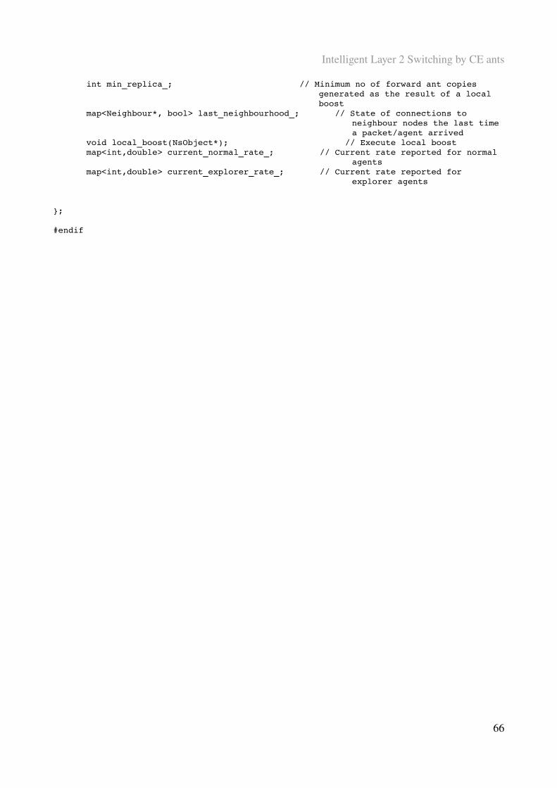
Intelligent Layer 2 Switching by CE ants
int min_replica_; // Minimum no of forward ant copies generated as the result of a local boost
map<Neighbour*, bool> last_neighbourhood_; // State of connections to neighbour nodes the last time a packet/agent arrived
void local_boost(NsObject*); // Execute local boostmap<int,double> current_normal_rate_; // Current rate reported for normal
agentsmap<int,double> current_explorer_rate_; // Current rate reported for
explorer agents
};
#endif
66
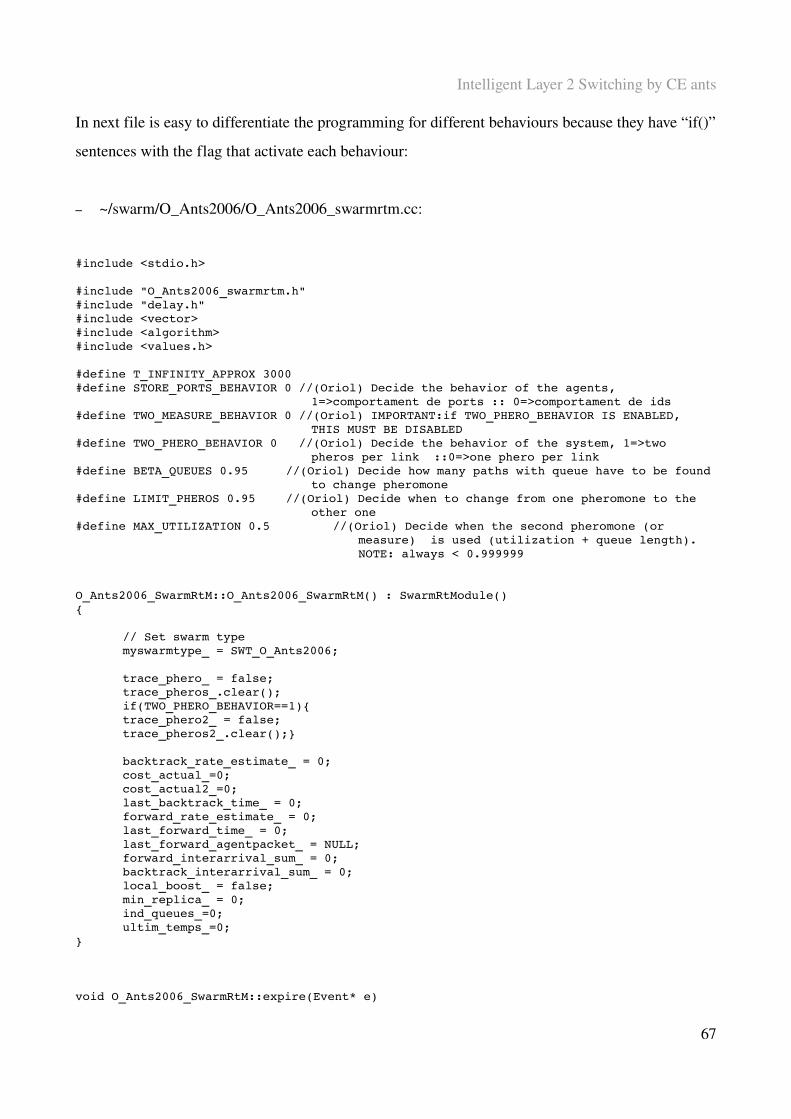
Intelligent Layer 2 Switching by CE ants
In next file is easy to differentiate the programming for different behaviours because they have “if()”
sentences with the flag that activate each behaviour:
– ~/swarm/O_Ants2006/O_Ants2006_swarmrtm.cc:
#include <stdio.h>
#include "O_Ants2006_swarmrtm.h"#include "delay.h"#include <vector>#include <algorithm>#include <values.h>
#define T_INFINITY_APPROX 3000#define STORE_PORTS_BEHAVIOR 0 //(Oriol) Decide the behavior of the agents,
1=>comportament de ports :: 0=>comportament de ids#define TWO_MEASURE_BEHAVIOR 0 //(Oriol) IMPORTANT:if TWO_PHERO_BEHAVIOR IS ENABLED,
THIS MUST BE DISABLED#define TWO_PHERO_BEHAVIOR 0 //(Oriol) Decide the behavior of the system, 1=>two
pheros per link ::0=>one phero per link#define BETA_QUEUES 0.95 //(Oriol) Decide how many paths with queue have to be found
to change pheromone#define LIMIT_PHEROS 0.95 //(Oriol) Decide when to change from one pheromone to the
other one#define MAX_UTILIZATION 0.5 //(Oriol) Decide when the second pheromone (or
measure) is used (utilization + queue length). NOTE: always < 0.999999
O_Ants2006_SwarmRtM::O_Ants2006_SwarmRtM() : SwarmRtModule(){
// Set swarm typemyswarmtype_ = SWT_O_Ants2006;
trace_phero_ = false;trace_pheros_.clear();if(TWO_PHERO_BEHAVIOR==1){trace_phero2_ = false;trace_pheros2_.clear();}
backtrack_rate_estimate_ = 0;cost_actual_=0;cost_actual2_=0;last_backtrack_time_ = 0;forward_rate_estimate_ = 0;last_forward_time_ = 0;last_forward_agentpacket_ = NULL;forward_interarrival_sum_ = 0;backtrack_interarrival_sum_ = 0;local_boost_ = false;min_replica_ = 0;ind_queues_=0;ultim_temps_=0;
}
void O_Ants2006_SwarmRtM::expire(Event* e)
67
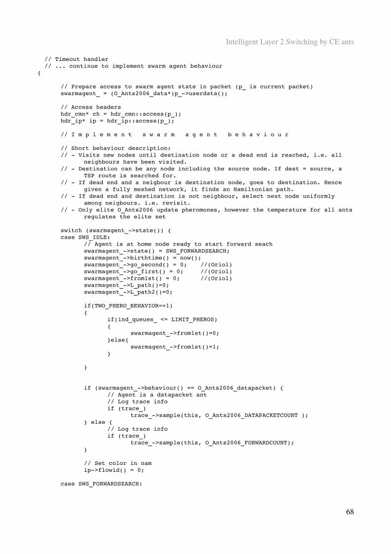
Intelligent Layer 2 Switching by CE ants
// Timeout handler // ... continue to implement swarm agent behaviour{
// Prepare access to swarm agent state in packet (p_ is current packet)swarmagent_ = (O_Ants2006_data*)p_>userdata();
// Access headershdr_cmn* ch = hdr_cmn::access(p_);hdr_ip* ip = hdr_ip::access(p_);
// I m p l e m e n t s w a r m a g e n t b e h a v i o u r
// Short behaviour description:// Visits new nodes until destination node or a dead end is reached, i.e. all
neighbours have been visited.// Destination can be any node including the source node. If dest = source, a
TSP route is searched for.// If dead end and a neigbour is destination node, goes to destination. Hence
given a fully meshed network, it finds an Hamiltonian path.// If dead end and destination is not neighbour, select next node uniformly
among neigbours. i.e. revisit.// Only elite O_Ants2006 update pheromones, however the temperature for all ants
regulates the elite set
switch (swarmagent_>state()) {case SWS_IDLE:
// Agent is at home node ready to start forward seachswarmagent_>state() = SWS_FORWARDSEARCH;swarmagent_>birthtime() = now();swarmagent_>go_second() = 0; //(Oriol)swarmagent_>go_first() = 0; //(Oriol)swarmagent_>from1st() = 0; //(Oriol)swarmagent_>L_path()=0;swarmagent_>L_path2()=0;
if(TWO_PHERO_BEHAVIOR==1){
if(ind_queues_ <= LIMIT_PHEROS){
swarmagent_>from1st()=0;}else{
swarmagent_>from1st()=1;}
}
if (swarmagent_>behaviour() == O_Ants2006_datapacket) {// Agent is a datapacket ant// Log trace infoif (trace_)
trace_>sample(this, O_Ants2006_DATAPACKETCOUNT );} else {
// Log trace infoif (trace_)
trace_>sample(this, O_Ants2006_FORWARDCOUNT);}
// Set color in namip>flowid() = 0;
case SWS_FORWARDSEARCH:
68
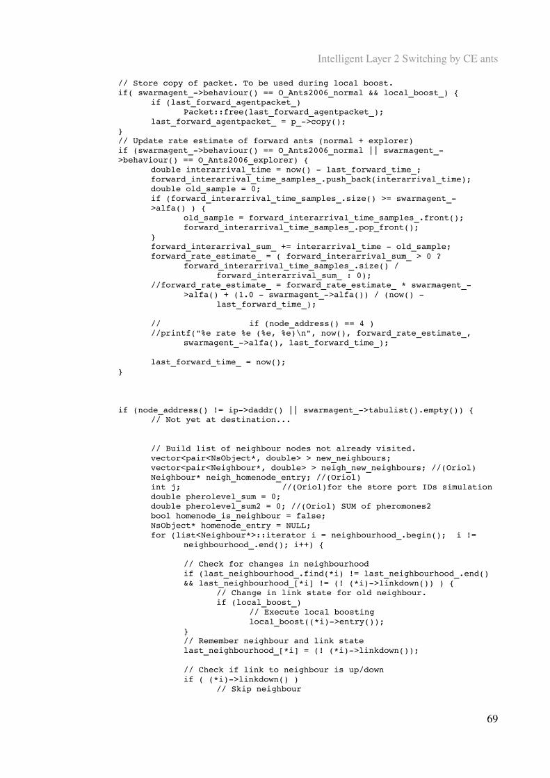
Intelligent Layer 2 Switching by CE ants
// Store copy of packet. To be used during local boost.if( swarmagent_>behaviour() == O_Ants2006_normal && local_boost_) {
if (last_forward_agentpacket_) Packet::free(last_forward_agentpacket_);
last_forward_agentpacket_ = p_>copy();}// Update rate estimate of forward ants (normal + explorer)if (swarmagent_>behaviour() == O_Ants2006_normal || swarmagent_>behaviour() == O_Ants2006_explorer) {
double interarrival_time = now() last_forward_time_;forward_interarrival_time_samples_.push_back(interarrival_time);double old_sample = 0;if (forward_interarrival_time_samples_.size() >= swarmagent_>alfa() ) {
old_sample = forward_interarrival_time_samples_.front();forward_interarrival_time_samples_.pop_front();
}forward_interarrival_sum_ += interarrival_time old_sample;forward_rate_estimate_ = ( forward_interarrival_sum_ > 0 ?
forward_interarrival_time_samples_.size() / forward_interarrival_sum_ : 0);
//forward_rate_estimate_ = forward_rate_estimate_ * swarmagent_>alfa() + (1.0 swarmagent_>alfa()) / (now()
last_forward_time_);
// if (node_address() == 4 )//printf("%e rate %e (%e, %e)\n", now(), forward_rate_estimate_,
swarmagent_>alfa(), last_forward_time_);
last_forward_time_ = now();}
if (node_address() != ip>daddr() || swarmagent_>tabulist().empty()) {// Not yet at destination...
// Build list of neighbour nodes not already visited.vector<pair<NsObject*, double> > new_neighbours;vector<pair<Neighbour*, double> > neigh_new_neighbours; //(Oriol)Neighbour* neigh_homenode_entry; //(Oriol)int j; //(Oriol)for the store port IDs simulationdouble pherolevel_sum = 0;double pherolevel_sum2 = 0; //(Oriol) SUM of pheromones2bool homenode_is_neighbour = false;NsObject* homenode_entry = NULL;for (list<Neighbour*>::iterator i = neighbourhood_.begin(); i !=
neighbourhood_.end(); i++) {
// Check for changes in neighbourhoodif (last_neighbourhood_.find(*i) != last_neighbourhood_.end() && last_neighbourhood_[*i] != (! (*i)>linkdown()) ) {
// Change in link state for old neighbour.if (local_boost_)
// Execute local boostinglocal_boost((*i)>entry());
}// Remember neighbour and link statelast_neighbourhood_[*i] = (! (*i)>linkdown());
// Check if link to neighbour is up/downif ( (*i)>linkdown() )
// Skip neighbour
69

Intelligent Layer 2 Switching by CE ants
continue;
// Check if neighbour has been visitedbool neighbour_visited = false;//(Oriol) Initial behavior, storing IDs in the agentif(STORE_PORTS_BEHAVIOR==0){
for (list<pair<nsaddr_t, NsObject*> >::iterator j = swarmagent_>tabulist().begin();
j != swarmagent_>tabulist().end(); j++) {if ( (*i)>addr() == j>first ) {
neighbour_visited = true; break;}
}}if(STORE_PORTS_BEHAVIOR==1)//behavior storing Ports in agent{
for (list<pair<nsaddr_t, NsObject*> >::iterator j = swarmagent_>tabulist().begin();
j != swarmagent_>tabulist().end(); j++) { list<pair<nsaddr_t, NsObject*> >::iterator prova=j;
prova++;if ( ((*i)>addr() == j>first) && ((prova)==swarmagent_>tabulist().end())) {
neighbour_visited = true; break;}
}
}
if (! neighbour_visited) {// Unvisited (new) neighbour found
if (TWO_PHERO_BEHAVIOR==0) //(Oriol) use of 1 pheromone behaviour
{// Find pheromone level (if any) towards neigbourPheroTableKey pk((*i)>entry(), swarmagent_>pheroid());PheroTable::iterator p = pherotable_.find(pk);pherolevel_sum += (p != pherotable_.end() ? (p>second).pherolevel() : 0);
// Store link entry towards neigbour and accumulated phero level towards neigbour
new_neighbours.push_back(pair<NsObject*, double>((*i)>entry(), pherolevel_sum));neigh_new_neighbours.push_back(pair<Neighbour*, double>(*i, 0));//
}
if (TWO_PHERO_BEHAVIOR==1)//use of 2 pheromones behavior
{// Find pheromone level (if any) towards neigbourif(swarmagent_>from1st()==0)//flag that means
which behavior have a particular agent, 0=> first pheromone :: 1=> second pheromone
70
Intelligent Layer 2 Switching by CE ants
{
PheroTableKey pk((*i)>entry(), swarmagent_>pheroid());PheroTable::iterator p = pherotable_.find(pk);pherolevel_sum += (p != pherotable_.end() ? (p>second).pherolevel() : 0);
// Store link entry towards neigbour and accumulated phero level towards neigbournew_neighbours.push_back(pair<NsObject*, double>((*i)>entry(), pherolevel_sum));
neigh_new_neighbours.push_back(pair<Neighbour*, double>(*i, 0));//(Oriol)
}else{
PheroTableKey pk((*i)>entry(), swarmagent_>pheroid());PheroTable::iterator p = pherotable2_.find(pk);pherolevel_sum2 += (p != pherotable2_.end() ? (p>second).pherolevel() : 0);
// Store link entry towards neigbour and accumulated phero level towards neigbournew_neighbours.push_back(pair<NsObject*, double>((*i)>entry(), pherolevel_sum2));
neigh_new_neighbours.push_back(pair<Neighbour*, double>(*i, 0));//(Oriol)
}}
}// Check if home node is neighbourif ( ! homenode_is_neighbour && (*i)>addr() == ip>daddr()) {
homenode_is_neighbour = true;homenode_entry = (*i)>entry();neigh_homenode_entry = *i;//(Oriol)
}}
// for the agents always can revisit all nodes in store ports behaviorif (STORE_PORTS_BEHAVIOR==0){
if (new_neighbours.empty()) {// All neighbours have been visitedif(homenode_is_neighbour) {
// Return to homenodenew_neighbours.push_back(pair<NsObject*, double>(homenode_entry, 1));neigh_new_neighbours.push_back(pair<Neighbour*, double>(neigh_homenode_entry, 0));pherolevel_sum = 1;if (TWO_PHERO_BEHAVIOR==1) pherolevel_sum2=1;
} else {// Allow revisit to any neighbourfor (list<Neighbour*>::iterator i = neighbourhood_.begin(); i !=
71

Intelligent Layer 2 Switching by CE ants
neighbourhood_.end(); i++) {new_neighbours.push_back(pair<NsObject*, double>((*i)>entry(), 0));
neigh_new_neighbours.push_back(pair<Neighbour*, double>(*i, 0));//(Oriol)}
}}
} if (STORE_PORTS_BEHAVIOR==1)//(Oriol){
if (new_neighbours.empty()) {for (list<Neighbour*>::iterator i = neighbourhood_.begin(); i != neighbourhood_.end(); i++) {
new_neighbours.push_back(pair<NsObject*, double>((*i)>entry(), 0));neigh_new_neighbours.push_back(pair<Neighbour*, double>(*i, 0));//(Oriol)
}}
}
// Select which neighbour to visit next by applying pheromone distribution
NsObject* nextnode = NULL;Neighbour* neigh_nextnode = NULL; //to save the next node in
neighbour formatif (TWO_PHERO_BEHAVIOR==0) {
if (pherolevel_sum == 0 || swarmagent_>behaviour() == O_Ants2006_explorer ) {
// No pheromones found or explorer behaviour set. Make a uniform distribution.
long n = randomgen_.rand_int(1, new_neighbours.size());nextnode = new_neighbours[n1].first;neigh_nextnode= neigh_new_neighbours[n1].first;//(Oriol)
} else {// Apply "roulett wheel" method base on pheromone
distribution to select next nodedouble u = randomgen_.uniform_double();j=0;//(Oriol)for (vector<pair<NsObject*, double> >::iterator i = new_neighbours.begin(); i != new_neighbours.end(); i++) {
//printf("<%e %d>, ", i>second, ((entry2neighbour_.find(i>first))>second)>addr());
if ( u <= (i>second / pherolevel_sum)) {// Select node to be nextnextnode = i>first;neigh_nextnode= neigh_new_neighbours[j].first;
break;}j++;
}}
}else{if ((pherolevel_sum == 0 && swarmagent_>from1st()==0) ||
72
Intelligent Layer 2 Switching by CE ants
(pherolevel_sum2 == 0 && swarmagent_>from1st()==1) || swarmagent_>behaviour() == O_Ants2006_explorer ) {
// No pheromones found or explorer behaviour set. Make a uniform distribution.
long n = randomgen_.rand_int(1, new_neighbours.size());nextnode = new_neighbours[n1].first;neigh_nextnode= neigh_new_neighbours[n1].first;//(Oriol)
} else {// Apply "roulett wheel" method base on pheromone
distribution to select next nodedouble u = randomgen_.uniform_double();j=0;for (vector<pair<NsObject*, double> >::iterator i = new_neighbours.begin(); i != new_neighbours.end(); i++) {
//printf("<%e %d>, ", i>second, ((entry2neighbour_.find(i>first))>second)>addr());if(swarmagent_>from1st()==0){
if ( u <= (i>second / pherolevel_sum)) {// Select node to be nextnextnode = i>first;
neigh_nextnode=neigh_new_neighbours[j].first;break;
}}else{
if ( u <= (i>second / pherolevel_sum2)) {// Select node to be nextnextnode = i>first;neigh_nextnode= neigh_new_neighbours[j].first;break;
}}j++;
}//printf("\n");
}}
//Update packetsize//ch>size() = swarmagent_>size() + sizeof(hdr_cmn) +
sizeof(hdr_swarm);//ch>size() *= 10; // Scale up a little to make packet visible in
nam//ch>size() = 1;if(swarmagent_>behaviour()!=O_Ants2006_datapacket){
if (STORE_PORTS_BEHAVIOR==0) ch>size() = ch>size() + 8*6; //(Oriol) Each node stored is 6 bytes MAC adress
else ch>size() = ch>size() + 8; // (Oriol) Maximum switches supposed of 256 ports
}else{ch>size()=1520;
}// Record current visit and entry to next node
swarmagent_>tabulist().push_back(pair<nsaddr_t, NsObject*>(node_address(), nextnode));
if (trace_phero_ && (trace_pheros_.empty() or
73

Intelligent Layer 2 Switching by CE ants
trace_pheros_.find(swarmagent_>pheroid()) != trace_pheros_.end() ) ) // Sample pheromone valuestrace_>sample(this, O_Ants2006_PHEROMONES );
//(Oriol) Touch to trace second pheromone (this and all the features)
if (TWO_PHERO_BEHAVIOR==1) //(Oriol){
if (trace_phero2_ && (trace_pheros2_.empty() or trace_pheros2_.find(swarmagent_>pheroid()) != trace_pheros2_.end() ) )
// Sample pheromone valuestrace_>sample(this, O_Ants2006_PHEROMONES2 );
}
//Here, the cost function has to be defined (Oriol)
//(Oriol) cost functions of Tdelay double utilization;
utilization= neigh_nextnode>traffic() / neigh_nextnode>bandwidth();printf("utilization=%lf \n", utilization);if(((swarmagent_>from1st()==0) && TWO_PHERO_BEHAVIOR==1) || TWO_PHERO_BEHAVIOR==0){
if(TWO_MEASURE_BEHAVIOR==0){
swarmagent_>L_path() = swarmagent_>L_path() + 100000000*1000*((ch>size()/neigh_nextnode>bandwidth())*(1/(1utilization)) + neigh_nextnode>retard());if (swarmagent_>L_path() ==0) swarmagent_>L_path()=0.000001;if (utilization > MAX_UTILIZATION && TWO_PHERO_BEHAVIOR==1) {
swarmagent_>go_second()=1;swarmagent_>go_first()=1;
}
}else{if(utilization<MAX_UTILIZATION){
//This cost is the transfer time exactly, but using a mean of utilization
swarmagent_>L_path() = swarmagent_>L_path() + 100000000*1000*((ch>size()/neigh_nextnode>bandwidth())*(1/(1utilization)) + neigh_nextnode>retard());
if (swarmagent_>L_path() ==0) swarmagent_>L_path()=0.000001;printf("Cost with cost function 1 is %lf, with cost function 2 would be %lf\n", 100000000*1000*((ch>size()/neigh_nextnode>bandwidth())*(1/(1utilization)) + neigh_nextnode>retard()), 100000000*1000*((ch>size()+neigh_nextnode>bitsQueueDrT())/neigh_nextnode
74

Intelligent Layer 2 Switching by CE ants
>bandwidth() + neigh_nextnode>retard()));}else{
//This is the real transfer time for a linkprintf("Cost with cost function 1 would be %lf, with cost function 2 is %lf\n", 100000000*1000*((ch>size()/neigh_nextnode>bandwidth())*(1/(1utilization)) + neigh_nextnode>retard()), 100000000*1000*((ch>size()+neigh_nextnode>bitsQueueDrT())/neigh_nextnode>bandwidth() + neigh_nextnode>retard()));//printf("llarg cua=%lf\n",neigh_nextnode>bitsQueueDrT());swarmagent_>L_path()=swarmagent_>L_path() + 100000000*1000*((ch>size() + neigh_nextnode>bitsQueueDrT())/neigh_nextnode>bandwidth() + neigh_nextnode>retard()); if (swarmagent_>L_path() ==0) swarmagent_>L_path()=0.000001;
}}
}else{
swarmagent_>L_path2() = swarmagent_>L_path2() + 100000000*1000*((ch>size() + neigh_nextnode>bitsQueueDrT())/neigh_nextnode>bandwidth() + neigh_nextnode>retard());if (swarmagent_>L_path2() ==0) swarmagent_>L_path2()=0.000001;if(utilization > MAX_UTILIZATION) {
swarmagent_>go_first()=1;swarmagent_>go_second()=1;
}}
// Move to next node (i.e. send agent state to next node)nextnode>recv(p_,h_);// Trigger local boost if appropriate//local_boost();
break;
} else {// Agent is at destination, prepare for backtracking
// Record current visit swarmagent_>tabulist().push_back(pair<nsaddr_t, NsObject*>(node_address(), NULL));
if (swarmagent_>behaviour() == O_Ants2006_datapacket) {// Agent is a datapacket ant, is simulation a datapacket// Log trace infoif (trace_){
trace_>sample(this, O_Ants2006_PATH | O_Ants2006_DATAPACKETRECEIVED | O_Ants2006_DATAPACKETCOST);if(TWO_PHERO_BEHAVIOR==1) trace_>sample(this,
75

Intelligent Layer 2 Switching by CE ants
O_Ants2006_DATAPACKETCOST2); //(Oriol)}// Terminate agentPacket::free(p_);break;
}
if (TWO_PHERO_BEHAVIOR==0){
if (gammaautoreg_.find(swarmagent_>pheroid()) == gammaautoreg_.end()) {
// First agent with this pheroid. Init misc variablesrho_reduction_factor_[swarmagent_>pheroid()] = 1;best_cost_[swarmagent_>pheroid()] = MAXDOUBLE; period_since_new_best_[swarmagent_>pheroid()] = 0;
}}else{
if (swarmagent_>from1st()==0){
if (gammaautoreg_.find(swarmagent_>pheroid()) == gammaautoreg_.end()) {
// First agent with this pheroid. Init misc variablesrho_reduction_factor_[swarmagent_>pheroid()] =1;best_cost_[swarmagent_>pheroid()] = MAXDOUBLE; period_since_new_best_[swarmagent_>pheroid()]=0;
}}else{
if (gammaautoreg2_.find(swarmagent_>pheroid()) == gammaautoreg2_.end()) {
// First agent with this pheroid. Init misc variablesrho_reduction_factor_[swarmagent_>pheroid()] =1;best_cost2_[swarmagent_>pheroid()] = MAXDOUBLE; period_since_new_best2_[swarmagent_>pheroid()] =0;
}}
}
// Calculate cost//double L_path = now() swarmagent_>birthtime();//(Oriol) Calculate cost due to swarmagent_>L_path() that has been
recorded during all the pathdouble L_path;if(TWO_PHERO_BEHAVIOR==0 || (TWO_PHERO_BEHAVIOR==1 && (swarmagent_>from1st()==0))){
L_path=swarmagent_>L_path();}else{
L_path=swarmagent_>L_path2();}
//if(now() > 268.0 && now() < 269.0 )// printf("%f L_path: %f Bh: %d\n", now(), L_path, swarmagent_>behaviour());
// Perform rhoreduction DISABLED// rho_reduction(L_path);
swarmagent_>rho() *= rho_reduction_factor_[swarmagent_>pheroid()];
76

Intelligent Layer 2 Switching by CE ants
// Calculate new temperature (gamma) for all agents //(Oriol) if (TWO_PHERO_BEHAVIOR==0 || (TWO_PHERO_BEHAVIOR==1 && ( swarmagent_>from1st()==0))) recalc_gamma(gammaautoreg_[swarmagent_>pheroid()], swarmagent_>L_path(), swarmagent_>beta(), swarmagent_>rho());
//(Oriol)if (TWO_PHERO_BEHAVIOR==1 && swarmagent_>from1st()==1) recalc_gamma(gammaautoreg2_[swarmagent_>pheroid()], swarmagent_>L_path2(), swarmagent_>beta(), swarmagent_>rho());
// Log trace infoif (trace_){
if (TWO_PHERO_BEHAVIOR==0) trace_>sample(this, O_Ants2006_GAMMA_ALL | O_Ants2006_ELITELIMIT | O_Ants2006_PATH | O_Ants2006_COST_ALL | O_Ants2006_ARRIVEDCOUNT);if (TWO_PHERO_BEHAVIOR==1) trace_>sample(this, O_Ants2006_GAMMA_ALL | O_Ants2006_ELITELIMIT | O_Ants2006_PATH | O_Ants2006_COST_ALL | O_Ants2006_ARRIVEDCOUNT | O_Ants2006_GAMMA_ALL2 | O_Ants2006_COST_ALL2);
}
// Check if path found is in "elite set"(Oriol)if(TWO_PHERO_BEHAVIOR==0 || TWO_PHERO_BEHAVIOR==1 && ( swarmagent_>from1st()==0)){
if ( swarmagent_>behaviour() == O_Ants2006_normal && swarmagent_>L_path() >= ( log(swarmagent_>rho()) * gammaautoreg_[swarmagent_>pheroid()].gamma())) {// Path not in elite set// Terminate agentPacket::free(p_);break;
}}else{
if ( swarmagent_>behaviour() == O_Ants2006_normal &&swarmagent_>L_path2() >= ( log(swarmagent_>rho()) * gammaautoreg2_[swarmagent_>pheroid()].gamma())) {// Path not in elite set// Terminate agentPacket::free(p_);break;
}}
// Calculate new temperatur (gamma) for elite agents (Oriol)if (TWO_PHERO_BEHAVIOR==0 || (TWO_PHERO_BEHAVIOR==1 && (swarmagent_>from1st()==0))){
recalc_gamma(gammaautoreg_elite_[swarmagent_>pheroid()], L_path, swarmagent_>beta(), swarmagent_>rho());// Store gamma and path cost as agent stateswarmagent_>gamma() = gammaautoreg_elite_[swarmagent_>pheroid()].gamma();//swarmagent_>L_path() = L_path;swarmagent_>gamma2() = gammaautoreg_elite2_[swarmagent_>pheroid()].gamma();
}if (TWO_PHERO_BEHAVIOR==1 && swarmagent_>from1st()==1){
recalc_gamma(gammaautoreg_elite2_[swarmagent_>pheroid()],
77
Intelligent Layer 2 Switching by CE ants
L_path, swarmagent_>beta(), swarmagent_>rho());// Store gamma and path cost as agent stateswarmagent_>gamma() = gammaautoreg_elite_[swarmagent_>pheroid()].gamma();swarmagent_>gamma2() = gammaautoreg_elite2_[swarmagent_>pheroid()].gamma();//swarmagent_>L_path2() = L_path;
}
// Set color in namip>flowid() = 1;// Reset ttlip>ttl() = swarmagent_>max_ttl();
// Log trace infoif (trace_){
if (TWO_PHERO_BEHAVIOR==0) trace_>sample(this, O_Ants2006_COST | O_Ants2006_GAMMA_ELITE | O_Ants2006_GAMMA_DIFF | O_Ants2006_GAMMA_REL | O_Ants2006_RHO | O_Ants2006_BACKTRACKCOUNT);
if (TWO_PHERO_BEHAVIOR==1) trace_>sample(this, O_Ants2006_COST | O_Ants2006_GAMMA_ELITE | O_Ants2006_GAMMA_DIFF | O_Ants2006_GAMMA_REL | O_Ants2006_RHO | O_Ants2006_BACKTRACKCOUNT | O_Ants2006_COST2 | O_Ants2006_GAMMA_ELITE2 | O_Ants2006_GAMMA_DIFF2 | O_Ants2006_GAMMA_REL2);
}//printf("Abans de passar backtracking a state");swarmagent_>state() = SWS_BACKTRACKING;// (... continous into next case ...)
}
case SWS_BACKTRACKING: {
// Get entry to previously visited node.NsObject* previous_node = swarmagent_>tabulist().back().second;
//printf("DEBUG bt %f %ld %d<", now(), (long)swarmagent_, node_address());//printf("Comenca el backtracking");if(previous_node) {
//printf ("%d ", ((entry2neighbour_.find(swarmagent_>tabulist().back().second))>second)>addr() );
// Update pheromones (Oriol)double L_on_gamma;if (TWO_PHERO_BEHAVIOR==0 || (TWO_PHERO_BEHAVIOR==1 && (swarmagent_>from1st()==0))){
if(swarmagent_>gamma()!=0) L_on_gamma = swarmagent_>L_path() / swarmagent_>gamma();else L_on_gamma = swarmagent_>L_path() / 0.000001;
}else{if(swarmagent_>gamma2()!=0) L_on_gamma = swarmagent_>L_path2() / swarmagent_>gamma2();else L_on_gamma = swarmagent_>L_path2() / 0.000001;
}double H = exp( L_on_gamma );for (list<Neighbour*>::iterator i = neighbourhood_.begin(); i != neighbourhood_.end(); i++) {
78
Intelligent Layer 2 Switching by CE ants
// Check if neighbour is node visited last timebool neigbour_is_last = ((*i)>entry() == previous_node);
// Update pheromones (Oriol)PheroAutoreg& p = pherotable_[PheroTableKey((*i)>entry(), swarmagent_>pheroid())];if (TWO_PHERO_BEHAVIOR==0 || (TWO_PHERO_BEHAVIOR==1 && (swarmagent_>from1st()==0))){
p = pherotable_[PheroTableKey((*i)>entry(), swarmagent_>pheroid())];p.pherolevel() = (neigbour_is_last? H : 0) +
p.A() + ( p.C() * p.B() == 0 || swarmagent_>gamma() > (2 * p.C() / p.B()) ?
p.B() / swarmagent_>gamma() + p.C() / (swarmagent_>gamma() * swarmagent_>gamma()) :
p.B() * p.B() / (4 * p.C() ) );}else{
p = pherotable2_[PheroTableKey((*i)>entry(), swarmagent_>pheroid())];
p.pherolevel() = (neigbour_is_last? H : 0) +p.A() + ( p.C() * p.B() == 0 || swarmagent_ >gamma2() > (2 * p.C() / p.B()) ?
p.B() / swarmagent_>gamma2() + p.C() / (swarmagent_>gamma2() * swarmagent_
>gamma2()) : p.B() * p.B() / (4 * p.C() ) );
}
// Check for "underflow"if (p.pherolevel() < 0) {
// Reset all phero parametersp.pherolevel() = 0;p.A() = 0;p.B() = 0;p.C() = 0;
} else {// Update pheromone autoreg parametersp.A() = swarmagent_>beta() * (p.A() + (neigbour_is_last ? H*(1+L_on_gamma * (1+L_on_gamma/2)) : 0) );if (TWO_PHERO_BEHAVIOR==0 || (TWO_PHERO_BEHAVIOR==1 && (swarmagent_>from1st()==0))){
p.B() = swarmagent_>beta() * (p.B() + (neigbour_is_last ? H*(swarmagent_>L_path() + swarmagent_>L_path() * swarmagent_>L_path() / swarmagent_>gamma() ) : 0) );p.C() = swarmagent_>beta() * (p.C() + (neigbour_is_last ? H*(swarmagent_>L_path() * swarmagent_>L_path() / 2 ) : 0) );
}else{p.B() = swarmagent_>beta() * (p.B() + (neigbour_is_last ? H*(swarmagent_>L_path2() + swarmagent_>L_path2() *
swarmagent_>L_path2() / swarmagent_>gamma2() ) : 0) );p.C() = swarmagent_>beta() * (p.C() +
79
Intelligent Layer 2 Switching by CE ants
(neigbour_is_last ? H*(swarmagent_>L_path2() * swarmagent_>L_path2() / 2 ) : 0) );
}
}}
}
// printf("\n");
// Update rate estimate of backtracking (elite) antsdouble interarrival_time = now() last_backtrack_time_;backtrack_interarrival_time_samples_.push_back(interarrival_time);double old_sample = 0;if (backtrack_interarrival_time_samples_.size() >= swarmagent_>alfa() ) {
old_sample = backtrack_interarrival_time_samples_.front();backtrack_interarrival_time_samples_.pop_front();
}backtrack_interarrival_sum_ += interarrival_time old_sample;backtrack_rate_estimate_ = (backtrack_interarrival_sum_ > 0 ? backtrack_interarrival_time_samples_.size() / backtrack_interarrival_sum_ : 0);//backtrack_rate_estimate_ = backtrack_rate_estimate_ * swarmagent_>alfa() + (1.0 swarmagent_>alfa()) / (now() last_backtrack_time_);last_backtrack_time_ = now();
// Remove current node from tabulistswarmagent_>tabulist().pop_back();if (swarmagent_>tabulist().empty()) {
// Backtracking completed//(Oriol) This is to check if there are a lot of paths with queueif(TWO_PHERO_BEHAVIOR==1){
if (swarmagent_>go_first()==0) swarmagent_>go_second()=0; //in order to change from queues to not queues
if( swarmagent_>go_second()==1){
ind_queues_=BETA_QUEUES*ind_queues_ + (1BETA_QUEUES)*1;}else{
ind_queues_=BETA_QUEUES*ind_queues_;}
}
// Terminate agentPacket::free(p_);break;
}
// Move to next nodeNeighbour* next_node = (addr2neighbour_.find( swarmagent_>tabulist().back().first ) )>second;if (next_node )
(next_node>entry())>recv(p_, h_);else
// Link between nodes in tabulist no longer existPacket::free(p_);
break;}default:
printf("O_Ants2006_SwarmRtM::runSwarmAgent: Invalide swarm agent state %d\n", swarmagent_>state());
80
Intelligent Layer 2 Switching by CE ants
Packet::free(p_);break;
}
// Process next queued packet (if any)poll_queue();
}
void O_Ants2006_SwarmRtM::rho_reduction(double L_path)// Adjust rho if when convergence is considered too slow
{if(! swarmagent_)
//Do nothingreturn;
/*if (swarmagent_>behaviour() == O_Ants2006_normal &&
gammaautoreg_.gamma() gammaautoreg_elite_.gamma() > swarmagent_>gammadiff_limit()) {// Difference between gamma for all agents and elite agents is exceeding
limit*/if (best_cost_[swarmagent_>pheroid()] > L_path) {
// New best costbest_cost_[swarmagent_>pheroid()] = L_path;period_since_new_best_[swarmagent_>pheroid()] = 0;
} elseperiod_since_new_best_[swarmagent_>pheroid()] += 1;
if (period_since_new_best_[swarmagent_>pheroid()] > swarmagent_>D() ) {// Adjust rho reduction factorrho_reduction_factor_[swarmagent_>pheroid()] *= 0.95;period_since_new_best_[swarmagent_>pheroid()] = 0;
// printf("%f Adjusting rho for %d: %le\n ", now(), swarmagent_>pheroid(), rho_reduction_factor_[swarmagent_>pheroid()]); fflush(NULL);
}
}
void O_Ants2006_SwarmRtM::recalc_gamma(GammaAutoreg& gammaauto, double L_path, double beta, double rho)
// Calculate new temperatur (gamma) and update autoreg parameters for gamma{
if (gammaauto.A() == 0 &&gammaauto.B() == 0 &&gammaauto.gamma() == 0 &&gammaauto.t() == 0)// Init. gammagammaauto.gamma() = L_path / log(rho);
double beta2t = 0;// A large t is approxed with t=infinity.if (gammaauto.t() < T_INFINITY_APPROX) {
gammaauto.t() += 1; beta2t = pow(beta, gammaauto.t());
}double L_on_gamma;if(gammaauto.gamma()!=0) L_on_gamma = L_path / gammaauto.gamma();else L_on_gamma = L_path / 0.000001;double H = exp( L_on_gamma );
double new_gamma = (gammaauto.B() + L_path * H) /
81
Intelligent Layer 2 Switching by CE ants
(gammaauto.A() + H * (1+ L_on_gamma) rho * ((1 beta2t)/(1 beta)));
// Check for "underflow"if (new_gamma > 0 )
gammaauto.gamma() = new_gamma;else
printf("O_Ants2006_SwarmRtM::recalc_gamma: Gamma less than 0 (%lf).\n", new_gamma);
// Update autoreg parameters for gammaif(gammaauto.gamma()!=0) L_on_gamma = L_path / gammaauto.gamma();else L_on_gamma = L_path / 0.000001;H = exp( L_on_gamma );
gammaauto.A() = beta * (gammaauto.A() + H * (1 + L_on_gamma));gammaauto.B() = beta * (gammaauto.B() + L_path * H);
}
float O_Ants2006_SwarmRtM::get_cost()// Return cost recoded by current swarm agent
{
return swarmagent_>L_path();
}
float O_Ants2006_SwarmRtM::get_cost2()// Return cost recoded by current swarm agent
{return swarmagent_>L_path2();
}
float O_Ants2006_SwarmRtM::get_gamma()// Return gamma (temperature) recoded by current swarm agent// This gamma is controlled by elite ants
{return swarmagent_>gamma();
}
float O_Ants2006_SwarmRtM::get_gamma2()// Return gamma (temperature) recoded by current swarm agent// This gamma is controlled by elite ants
{return swarmagent_>gamma2();
}
float O_Ants2006_SwarmRtM::get_gamma_all()// Return gamma (temperature) updated by all ants
{return gammaautoreg_[swarmagent_>pheroid()].gamma();
}
float O_Ants2006_SwarmRtM::get_gamma_all2()// Return gamma (temperature) updated by all ants
{return gammaautoreg2_[swarmagent_>pheroid()].gamma();
}
list<pair<nsaddr_t,NsObject*> >& O_Ants2006_SwarmRtM::get_path()
82
Intelligent Layer 2 Switching by CE ants
// Return path traversed by current swarm agent{
return swarmagent_>tabulist();}
float O_Ants2006_SwarmRtM::get_delay()// Return delay experienced by current swarm agent
{return 0;
}
float O_Ants2006_SwarmRtM::get_elitelimit()// Return limit for being in elite set
{return ( log(swarmagent_>rho()) * gammaautoreg_[swarmagent_
>pheroid()].gamma());}
float O_Ants2006_SwarmRtM::get_elitelimit2()// Return limit for being in elite set
{return ( log(swarmagent_>rho()) * gammaautoreg2_[swarmagent_
>pheroid()].gamma());}
float O_Ants2006_SwarmRtM::get_rho()// Return rho applied
{return swarmagent_>rho();
}
int O_Ants2006_SwarmRtM::get_pheroid()// Return pheromone id
{return swarmagent_>pheroid();
}
int O_Ants2006_SwarmRtM::get_behaviour()// Return behaviour flag (0 = normal, 1 = explorer){
return swarmagent_>behaviour();}
map<nsaddr_t, double>& O_Ants2006_SwarmRtM::get_phero() // Return current pheromone value for current agent
{phero_list_.clear();
for (list<Neighbour*>::iterator i = neighbourhood_.begin(); i != neighbourhood_.end(); i++) {// Find pheromone level (if any) for current agent towards neigbourPheroTableKey pk((*i)>entry(), swarmagent_>pheroid());PheroTable::iterator p = pherotable_.find(pk);phero_list_[((entry2neighbour_.find((*i)>entry()))>second)>addr()] =
(p != pherotable_.end() ? (p>second).pherolevel() : 0);}
return phero_list_;}
map<nsaddr_t, double>& O_Ants2006_SwarmRtM::get_phero2() //(Oriol)// Return current pheromone value for current agent
{phero_list2_.clear();
83
Intelligent Layer 2 Switching by CE ants
for (list<Neighbour*>::iterator i = neighbourhood_.begin(); i != neighbourhood_.end(); i++) {
// Find pheromone level (if any) for current agent towards neigbourPheroTableKey pk((*i)>entry(), swarmagent_>pheroid());PheroTable::iterator p = pherotable2_.find(pk);phero_list2_[((entry2neighbour_.find((*i)>entry()))>second)>addr()] = (p != pherotable2_.end() ? (p>second).pherolevel() : 0);
}
return phero_list_;}
double O_Ants2006_SwarmRtM::get_backtrack_rate()// Return estimated rate of backtracking agents
{return backtrack_rate_estimate_;
}
void O_Ants2006_SwarmRtM::local_boost(NsObject* failed_link_entry)// Execute local boost if required, i.e. generate a set of additional forward agents{
// Prepare prob. dist. (pdf) based on "pheromones"vector<pair<NsObject*, double> > neighbours;double pherolevel_sum = 0;for (list<Neighbour*>::iterator i = neighbourhood_.begin(); i != neighbourhood_.end(); i++) {
// Check if link to neighbour is up/downif ( (*i)>linkdown() )
// Skip neighbourcontinue;
// Find pheromone level (if any) towards neigbourPheroTableKey pk((*i)>entry(), swarmagent_>pheroid());PheroTable::iterator p = pherotable_.find(pk);double phero_level=(p != pherotable_.end() ? (p>second).pherolevel() : 0);pherolevel_sum += phero_level;
// Store link entry towards neigbour and accumulated phero level towards neigbour
neighbours.push_back(pair<NsObject*, double>((*i)>entry(), phero_level));}
// Get pheromone level on failed link tooPheroTableKey pk(failed_link_entry, swarmagent_>pheroid());PheroTable::iterator p = pherotable_.find(pk);double phero_level_failed_link = (p != pherotable_.end() ? (p>second).pherolevel() : 0);
// Calculate size of boost (equ. 9 in paper, and rate weighted by pheromonlevel on failed link)
double current_rate = ((O_Ants2006_data*)last_forward_agentpacket_>userdata())>current_rate();double rate_weight = phero_level_failed_link / (pherolevel_sum + phero_level_failed_link);double boost_size = min_replica_ *
( 1 + (neighbourhood_.size() 1 ) * (forward_rate_estimate_ * rate_weight / current_rate));
printf("%f local boost at %d:\n\tForward rate estimate %f\n\tCurrent rate %f\n\tRate weight %f\n\tBoost size %f\n\tBoost distr.: ", now(), node_address(), forward_rate_estimate_, current_rate,
84
Intelligent Layer 2 Switching by CE ants
rate_weight, boost_size);
for (vector<pair<NsObject*, double> >::iterator i = neighbours.begin(); i != neighbours.end(); i++) {
// Generate a boost of agents relative to pheromone level towards neighbourint num_agents = (int)( boost_size * (i>second / pherolevel_sum) );
// Generate boosts of agents. Apply uniform distribution.//int num_agents = (int)(boost_size / neighbours.size() );
num_agents = (num_agents > 0 ? num_agents : 1 ); // Round up
printf("%d >%d, ", num_agents, ((entry2neighbour_.find(i>first))>second)>addr());
for (int j=0; j < num_agents; j++) {
// Prepare copy of last forward agent sentPacket* p = last_forward_agentpacket_>copy();
// Send packet(i>first)>recv(p,h_);
}}printf("\n"); fflush(NULL);
}
85