i

Intelligent Distribution Voltage Control in The Presence of

Intermittent Embedded Photo-Voltaic Generation

 

A thesis submitted in fulfilment of the requirements for the degree of

Doctor of Philosophy

Kai Cheung Peter Wong B.Sc.(Eng.), CPEng, FIEAust, SMIEEE, MIET

College of Engineering and Science

Victoria University

PO Box 14428

Melbourne

Victoria, Australia, 8001

March 2017

ii

To my beloved family,

Thank you for your support and encouragement during the course of the PhD study.

Without your support, this thesis will not be possible.

iii

Table of Contents Declaration of Originality ............................................................................................................ i

Acknowledgments ................................................................................................................... …ii

List of Figures ............. …………………………………………………………………………iii

List of Tables …………………………………………………………………………………vii

List of Nomenclature ............... …………………………………………………………………ix

List of Publications ............ …………………………………………………………………...xiii

Abstract…………………………………………………………………….………...... ............ xi

Chapter 1 -  Introduction ......................................................................................................... 1 

  Overview ....................................................................................................................... 1 

  Key Objectives .............................................................................................................. 4 

  Design and Methodology .............................................................................................. 5 

  Literature Review .................................................................................................. 5 

  Methodology ......................................................................................................... 6 

  Research Significance ................................................................................................... 7 

  Original Contribution .................................................................................................... 7 

  Thesis Organisation ....................................................................................................... 8 

  Summary ....................................................................................................................... 9 

Chapter 2 -  Literature Review .............................................................................................. 10 

  Overview ..................................................................................................................... 10 

  Quality of Supply in the Low Voltage Networks ........................................................ 10 

  Impact of Grid Connected PV Systems ....................................................................... 11 

  Voltage Quality Data from Smart Meters ................................................................... 12 

  Network Modelling Techniques .................................................................................. 13 

  Methods to Increase the Hosting Capacity of LV Networks for PV Generators ........ 15 

  Key Issues Identified ................................................................................................... 17 

  Summary ..................................................................................................................... 18 

Chapter 3 -  Exploratory Analysis of Smart Meter Voltage Quality Data ........................ 19 

  Overview ..................................................................................................................... 19 

  Smart Meter Rollout Program ..................................................................................... 19 

  Forms of Smart Meter Voltage Quality Data .............................................................. 20 

  Exploratory Analysis of Smart Meter Voltage Quality Data ...................................... 21 

  Data Set ............................................................................................................... 21 

  Analysis of Undervoltage Events ........................................................................ 22 

  Analysis of Overvoltage Events .......................................................................... 26 

iv

  Relationship Between Overvoltage and Embedded Photovoltaic Generation .... 30 

  Relationship Between Voltage Non-compliance and Customer Complaints ...... 32 

  Linking Voltage Quality Events to Supply Substations .............................................. 32 

  Undervoltage Sites .............................................................................................. 33 

  Overvoltage Sites ................................................................................................ 35 

  Sites Experiencing both Overvoltage and Undervoltage ..................................... 37 

  A Big Data Problem .................................................................................................... 38 

  Summary ..................................................................................................................... 38 

Chapter 4 -  A PV Generator Model Suitable for Practical Utility Applications ............. 41 

  Overview ..................................................................................................................... 41 

  Survey of Existing PV Generator Models ................................................................... 42 

  Solar Cell Modelling [26, 27, 62-67] .................................................................. 42 

  Inverter Modelling [67-70] .................................................................................. 47 

  Solar Irradiance Modelling [67, 71, 72] .............................................................. 47 

  Overall PV generator model ................................................................................ 48 

  Need for a Simplified Generator Model for Residential Roof-top PV Systems . 48 

  Simplified Generator Model for Residential Roof-top PV Systems ........................... 49 

  Insight from Smart Meter Data ........................................................................... 49 

  Derivation of a Simplified PV Generator Model ................................................ 52 

  Applications of the Simplified PV Generator Model .................................................. 54 

  Solar Irradiance Data at PV Locations ................................................................ 54 

  Modelled and Actual Output of a PV System ..................................................... 57 

  Power Quality Investigations .............................................................................. 59 

  Gross and Net Load Profiles ............................................................................... 60 

  Summary ..................................................................................................................... 62 

Chapter 5 -  LV Network Model for Simulation Studies .................................................... 64 

  Overview ..................................................................................................................... 64 

  Network Asset Data .................................................................................................... 65 

  Derivation of Line Impedances ................................................................................... 66 

  The Need to Model Neutral Conductor and Earth ............................................... 66 

  Calculating LV Line Impedances Considering Neutral Conductor and Earth .... 67 

  Derivation of Loads and Generation ........................................................................... 70 

  Load Modelling ................................................................................................... 70 

  Generation Modelling ......................................................................................... 72 

  Modelling of Voltage Control Devices ....................................................................... 73 

v

  Modelling Software ..................................................................................................... 73 

  Network Scenarios Modelled ...................................................................................... 76 

  Summary ..................................................................................................................... 80 

Chapter 6 -  Analysis of Simulation Results ......................................................................... 81 

  Overview ..................................................................................................................... 81 

  Effect of MV Voltage Regulation Control .................................................................. 82 

  OLTC Flat Voltage Control ................................................................................ 82 

  Line Drop Compensation .................................................................................... 85 

  Mixed Load Types .............................................................................................. 86 

  Effect of LV Voltage Regulation Control ................................................................... 87 

  LV Model to Include Effects of Circuit unbalance, Load Unbalance and Ground

Connections ......................................................................................................... 87 

  LV PV Generation Caused Localized Voltage Rise and Voltage Unbalance ..... 88 

  Phase Voltage Unbalance, Its Effect and Applicable Standards ................................. 88 

  Optimal Solar Generator Placement to Reduce Voltage Unbalance ........................... 90 

  Smart Grid Voltage Control Technologies .................................................................. 93 

  Smart Grid Distribution Transformer fitted with On-load Tap Changer (OLTC)

and Automatic Voltage Control Scheme ............................................................. 93 

  Smart PV Inverters .............................................................................................. 95 

  Connect Battery Storage to PV Generator ........................................................ 101 

  Future Scenario of Higher PV Penetration ................................................................ 104 

  Summary ................................................................................................................... 108 

Chapter 7 -  Conclusions and Future Research ................................................................. 109 

  Overview ................................................................................................................... 109 

  Conclusions ............................................................................................................... 109 

  Future Work and Recommendation .......................................................................... 115 

  Concluding Remarks ................................................................................................. 116 

Appendices – OpenDSS & MatLab Codes ............................................................................ 118 

  OpenDSS codes for network model .......................................................................... 118 

  MATLAB Codes for Phase Voltage Analysis .......................................................... 121 

  MATLAB Codes for Voltage Unbalance Analysis ................................................... 128 

References 135 

i

Declaration of Originality

I, Kai Cheung Peter Wong, declare that the PhD thesis entitled “Intelligent Distribution

Voltage Control in The Presence of Intermittent Embedded Photo-Voltaic Generation” is

no more than 100,000 words in length including quotes and exclusive of tables, figures,

appendices, bibliography, references and footnotes. This thesis contains no material that

has been submitted previously, in whole or in part, for the award of any other academic

degree or diploma. Except where otherwise indicated, this thesis is my own work.

Signature Date

Kai Cheung Peter Wong 15 March 2017

ii

Acknowledgment

Someone once said that a Doctoral research was a lonely journey. In the pursuit of

extending the boundary of human understanding, a PhD candidate often finds himself or

herself in places where no one has ever been before. I am fortunate to have pick a research

topic that is in the front of minds of many engineers practising in the electricity supply

industry. Discussions with these engineers during my course of employment and in

industry conferences have all contributed to ideas presented in this thesis. To these “un-

named” engineers I offer my gratitude.

I would like to thank Professor Akhtar Kalam of Victoria University for persuading me

to take up the research and offering me sound advice along the way. Dr Robert Barr,

principal of Electric Power Consulting, agreed to be my industry supervisor and his

practical insight has been invaluable. My employer, Jemena, has been very supportive of

my academic research and has contributed relevant industry data. To my cohort of PhD

students at Victoria University, their comradeship and practical help has been

outstanding.

No success, however, will come without the emotional support of my family. I would like

to thank my wife Ada who has gracefully accepted my many working weekends and

working holidays so progress can be made in my PhD research while I am employed full-

time. My son Geoffrey has offered practical help around the house when I am desk-bound

and his sense of humour has brightened up many stressful situations. To Engineers

Australia who awarded me the John Madsen Medal for the best paper published in the

Australian Journal of Electrical & Electronics Engineering (2015) – it’s like a shot of

adrenalin in the arm close to the finishing line!

Last but not least, the human minds have been created with the capacity to pursue

knowledge and understanding about the natural laws that govern the behaviour of things

on earth. To this Creator I offer my deepest gratitude.

iii

List of Figures

Fig. 1.1. A residential roof-top PV installation ............................................................................. 2 

Fig. 1.2. Augmentation expenditure of JEN .................................................................................. 2 

Fig. 1.3. Typical load curves for three classes of customers during summer peak ....................... 3 

Fig. 2.1. Long-term national power quality survey result for steady state voltages of LV sites

(2013-14) ........................................................................................................................ 11 

Fig. 2.2. Typical voltage regulation schemes in Australia .......................................................... 16 

Fig. 3.1. Advanced Metering Infrastructure installed by Jemena Electricity Networks ............. 20 

Fig. 3.2. Example of event list for overvoltage events ................................................................ 20 

Fig. 3.3. Parameters associated with a voltage quality event ...................................................... 21 

Fig. 3.4. Number of active undervoltage sites during the 6-day period ...................................... 23 

Fig. 3.5. Number of undervoltage events versus maximum daily ambient temperature ............. 24 

Fig. 3.6. Number of undervoltage events versus start times ....................................................... 25 

Fig. 3.7. Number of undervoltage events versus duration (minutes) .......................................... 25 

Fig. 3.8. Minimum voltage of undervoltage events .................................................................... 26 

Fig. 3.9. Number of active overvoltage sites during the 6-day period ........................................ 27 

Fig. 3.10. Percentage of sites giving overvoltage events versus maximum daily ambient

temperature ..................................................................................................................... 28 

Fig. 3.11. Number of overvoltage events versus start times ....................................................... 29 

Fig. 3.12. Number of overvoltage events versus duration (minutes) .......................................... 29 

Fig. 3.13. Maximum voltage of overvoltage events .................................................................... 30 

Fig. 3.14. Growth of residential PV systems in JEN ................................................................... 31 

Fig. 3.15. Analysis of customer voltage complaints ................................................................... 32 

Fig. 3.16. Linking OV sites to upstream supply substations ....................................................... 33 

iv

Fig. 4.1. Equivalent circuit of a PV cell (5-parameter model) .................................................... 42 

Fig. 4.2. Simplified 4-parameter model of a PV cell .................................................................. 43 

Fig. 4.3. Example of data required to set up a PV output model in a commonly used engineering

software package ............................................................................................................ 46 

Fig. 4.4. I-V and P-V characteristics of a PV array at different irradiance levels ....................... 46 

Fig. 4.5. Energy demand data of a customer with a 1kW PV system ......................................... 49 

Fig. 4.6. Consumption data for a customer ................................................................................. 50 

Fig. 4.7. PV generation data for a customer ................................................................................ 50 

Fig. 4.8. Maximum power output of a number of PV sites over the course of one year ............. 51 

Fig. 4.9. Map of Jemena Electricity Networks ............................................................................ 54 

Fig. 4.10. Daily correlation coefficients for the 1kW PV customer site ..................................... 55 

Fig. 4.11. Components of solar irradiance on a day where strong correlation is found between

solar irradiance and PV generation ................................................................................ 56 

Fig. 4.12. Components of solar irradiance on a day where weak correlation is found between solar

irradiance and PV generation ......................................................................................... 56 

Fig. 4.13. Actual and estimated output of a 1kW PV system on a relatively cloudy day ........... 58 

Fig. 4.14. Actual and estimated output of a 1kW PV system on a relatively clear sky day ........ 59 

Fig. 4.15. Model voltage output of a 5 kW PV system in a power quality investigation ............ 60 

Fig. 4.16. Estimated and measured load profile for the 1kW PV site ......................................... 62 

Fig. 5.1. LV Distribution Circuits from Cypress Stillia Distribution Substation ........................ 66 

Fig. 5.2. Details of LV Distribution Circuit #4 ........................................................................... 66 

Fig. 5.3. Concepts of conductor images used in Carson’s equations .......................................... 68 

Fig. 5.4. Weekly loadshapes used in the simulation based on SCADA and smart meter

measurements ................................................................................................................. 71 

v

Fig. 5.5. Loadshapes used in the simulation for 15 February 2015 based on SCADA and smart

meter measurements ....................................................................................................... 72 

Fig. 5.6 Output of solar generator PV1 between 15 to 21 February 2015 .................................. 72 

Fig. 5.7. Example OpenSS codes for converting a 4-wre LV line construction into impedance

matrix ............................................................................................................................. 74 

Fig. 5.8. Output of OpenDSS codes for a 4-wire LV line ........................................................... 74 

Fig. 5.9. Single-line presentation of network model ................................................................... 76 

Fig. 5.10. SCADA readings of loads on SHM Zone Substation and SHM14 feeder .................. 77 

Fig. 5.11. Commercial and industrial loadshapes for the period 15 to 21 Feb 2015 ................... 78 

Fig. 6.1. Red phase voltage on 433V side of distribution substation showing the effect of various

MV voltage control schemes (Scenarios 1, 2, 4, 5 & 6) ................................................. 84 

Fig. 6.2. Voltages at the end of LV distribution circuit #4 .......................................................... 84 

Fig. 6.3. The use of Line Drop Compensation has improved the voltage at the 433V side of the

distribution substation (Bus9) ........................................................................................ 85 

Fig. 6.4. The use of Line Drop Compensation has improved the voltage at the end of LV circuit

#4 (Bus17) ...................................................................................................................... 85 

Fig. 6.5. Red phase voltage on 433V side of distribution substation showing the effect of different

load profiles on SHM 22kV bus ..................................................................................... 86 

Fig. 6.6. Voltages at the end of LV distribution circuit #4, with MV and LV network modelled as

3-wire balanced network ................................................................................................ 87 

Fig. 6.7. Voltages at the end of LV distribution circuit #4 .......................................................... 88 

Fig. 6.8. Modelled results with PV1 and PV2 both connected to red phase ............................... 92 

Fig. 6.9. Modelled results with PV1 connected to white phase and PV2 connected to blue phase

........................................................................................................................................ 93 

Fig. 6.10. Voltages at 415V bus (Bus9) with OLTC distribution transformer ............................ 94 

vi

Fig. 6.11. Voltages at end of distribution circuit #4 (Bus17) with OLTC distribution transformer

........................................................................................................................................ 94 

Fig. 6.12. Voltage unbalance on various load buses with OLTC distribution transformer ......... 94 

Fig. 6.13. Volt-Watt characteristics of smart inverter used in the simulation ............................. 96 

Fig. 6.14. Effect of Smart Inverter Volt-Watt control on phase voltages ................................... 97 

Fig. 6.15. Effect of Smart Inverter Volt-Watt control on voltage unbalance .............................. 97 

Fig. 6.16. Volt-Var characteristics of smart inverter used in the simulation ............................... 98 

Fig. 6.17. Effect of Smart Inverter Volt-Var control on phase voltages ..................................... 99 

Fig. 6.18. Effect of larger inverter rating on Smart Inverter Volt-Var control .......................... 100 

Fig. 6.19. Effect of larger inverter rating on voltage unbalance ................................................ 100 

Fig. 6.20. Charging & discharging characteristics of the 4.4kW/25kWh battery. .................... 102 

Fig. 6.21. Battery energy and charging status during the simulation. ....................................... 103 

Fig. 6.22. Voltages at Bus20 without storage battery ............................................................... 104 

Fig. 6.23. Voltages at Bus20 with storage battery ..................................................................... 104 

Fig. 6.24. Voltage unbalance on the load buses with storage battery ....................................... 104 

Fig. 6.25. Voltages at the various load buses with four PV ...................................................... 105 

Fig. 6.26. Voltages at the various load buses with four PV and after phase optimisation ........ 106 

Fig. 6.27. Voltages at the various load buses with four PV and after phase optimisation and

application of LDC ....................................................................................................... 107 

vii

List of Tables

Table 3.1 Undervoltage events .................................................................................................... 23 

Table 3.2 Analysis of the 6,131 undervoltage sites ..................................................................... 23 

Table 3.3 Overvoltage events ...................................................................................................... 27 

Table 3.4 Analysis of the 6,131 overvoltage sites ....................................................................... 27 

Table 3.5 Proportion of overvoltage events generated by sites with PV installation .................. 31 

Table 3.6 20 distribution substations with the highest percentage of undervoltage sites in the 6-

day period ....................................................................................................................... 34 

Table 3.7 Ten worst zone substations which supply distribution substations with undervoltage

events ............................................................................................................................. 35 

Table 3.8 20 distribution substations with the highest percentage of overvoltage sites in the 6-

day period ....................................................................................................................... 36 

Table 3.9 Ten worst zone substations which supply distribution substations with overvoltage

events ............................................................................................................................. 37 

Table 3.10 Seven worst distribution substations whose customers have experienced both

overvoltage and undervoltage events in the 6-day period .............................................. 37 

Table 4.1 Summary of correlation coefficients .......................................................................... 55 

Table 5.1 Network Characteristics (provided by Jemena Electricity Networks) ...................... 65 

Table 5.2 Derivation of base loads and load shapes ................................................................. 71 

Table 5.3 Voltage Control Devices .......................................................................................... 73 

Table 5.4 Impedance Matrix for 4-wire 19/3.25AAC LV Overhead Line ............................... 75 

Table 5.5 Network Scenarios for MV Voltage Control ........................................................... 79 

Table 5.6 Network Scenarios for LV Voltage Control ............................................................ 79 

Table 6.1 Voltage Control Settings .......................................................................................... 83 

viii

Table 6.2 Network Voltage Unbalance Factor for Different Combinations of Phase Connection

of Generators PV1 and PV2 ........................................................................................... 92 

Table 6.3 Network Voltage Unbalance Factor for Different Combinations of Phase Connection

of Generators PV1 and PV2, with PV3 and PV4 connected to Customer 6 (W-phase) and

Customer 2 (B-phase) .................................................................................................. 106 

ix

List of Nomenclature

AC Alternating Current

ADMD After Diversity Maximum Demand

AMI Advanced Metering Infrastructure

BOM Bureau of Meteorology

COM Component Object Model

DC Direct Current

DSTATCOM Distribution Static Compensator

GIS Geographical Information System

HANA High Performance Analytical Appliance, an in-memory processing database

in the SAP suite of products

IEC International Electrotechnical Commission

JEN Jemena Electricity Networks

kVA Kilo-Volt-Ampere, a measure of energy

kW Kilo-Watt, a measure of active power

kWh Kilo-Watt hour, a measure of active energy

LDC Line Drop Compensation

LV Low Voltage

MATLAB Matrix Laboratory, a multi-paradigm numerical computing environment and

fourth-generation programming language

MEN Multiple Earthed Neutral

MPPT Maximum Power Point Tracking

MV Medium Voltage

MVA Mega-Volt-Ampere, a measure of energy

MWh Mega-Watt hour, a measure of active energy

NOCT Nominal Operating Cell Temperature

OLTC On-Load Tap Changer

OpenDSS Open Distribution System Simulator

x

OV Overvoltage

PDF Probability Density Function

POA Plane-of-array

POC Point of Connection

PQ Loads Loads expressed in active power (P) and reactive power (Q)

PV Photo-Voltaic

SAP Systems, Applications and Products, a software for enterprise resource

planning and data management

SCADA Supervisory Control and Data Acquisition

STC Standard Test Conditions

TMY Typical Meteorological Year

UV Undervoltage

VRR Voltage Regulating Relay

xi

List of Publications

1. P.K.C. Wong, R.A. Barr and A. Kalam, “Analysis of Voltage Quality Data from

Smart Meters”, Australasian Universities Power Engineering Conference, 2012

2. R.A. Barr, P. Wong and A. Baitch, “New Concepts for Steady State Voltage

Standards”, IEEE International Conference on Harmonics & Quality of Power, 2012

3. P.K.C. Wong, R.A. Barr and A. Kalam, “Using smart meter data to improve quality

of voltage delivery in public electricity distribution networks”, Saudi Arabia Smart

Grid Conference, 2012

4. Peter K.C. Wong, Akhtar Kalam and Robert Barr, “A Big Data Challenge – Turning

Smart Meter Voltage Quality Data into Actionable Information”, 22nd International

Conference on Electricity Distribution (CIRED), 2013

5. Peter K.C. Wong, Robert A. Barr, Akhtar Kalam, “Voltage Rise Impacts and

Generation Modeling of Residential Roof-top Photo-Voltaic Systems”, IEEE

International Conference on Harmonics & Quality of Power, 2014

6. Peter K.C. Wong, Akhtar Kalam and Robert Barr, “Generation Modeling of

Residential Roof-top Photo-Voltaic Systems”, 23rd International Conference on

Electricity Distribution (CIRED), 2015

7. Peter K.C. Wong, Robert A. Barr & Akhtar Kalam, “Generation modelling of

residential rooftop photovoltaic systems and its applications in practical electricity

distribution networks”, Australian Journal of Electrical and Electronics Engineering,

12:4, 332-341. The paper was awarded the John Madsen Medal for the best paper

published in AJEEE in 2015.

8. Peter K.C. Wong, Akhtar Kalam and Robert Barr, “Modelling and Analysis of

Practical Options to Improve the Hosting Capacity of Low Voltage Networks for

Embedded Photo-Voltaic Generation”, accepted for publication in the IET (Institution

of Engineering & Technology) Journal of Renewable Power Generation. Doi:

10.1049/iet-rpg.2016.0770.

9. Peter K.C. Wong, Akhtar Kalam, Robert A. Barr, “Increase the hosting capacity of

four-wire low-voltage supply network for embedded solar generators by optimising

generator and load placement on the three supply phases”, 24th International

Conference & Exhibition on Electricity Distribution (CIRED), 2017

xii

Abstract

Dwindling fossil fuel resources and the concern for greenhouse gas emissions resulting

from the burning of fossil fuels have led to significant development of renewable energy

in many countries. While renewable energy takes many forms, solar and wind resources

are being harvested in commercial scale in many parts of the world. Government

incentives such as Renewable Energy Certificates and Feed-in Tariffs have contributed

to the rapid uptake.

Australia, per capita of population, has topped the world in the penetration of residential

roof-top solar generation systems. With electricity consumers of only 10 million, there

are almost 1.5 million grid connected residential solar installations approaching

5,000MW of installed capacity in June 2016, and the number continues to grow. These

residential PV generations are embedded in the Low Voltage (LV) networks that were

traditionally designed to take one-way flow of electricity only. As the number of

embedded solar generators increases, customers begin to experience voltage quality

problems.

Public electricity supply networks are required to deliver voltages within narrow ranges.

This ensures that the supply voltages are compatible with the design parameters of

consumer electrical equipment. Supply voltage non-compliance has high societal costs as

it impacts on the efficiency, performance and life expectancy of electrical equipment.

Except for large commercial or industrial customers, however, direct monitoring of the

quality of voltage delivered is not possible due to the relatively high cost of providing

measurement at each customer’s point of supply. Electricity distribution utilities

generally adopt a reactive approach of responding to customer voltage complaints. This

approach could be appropriate if it is expected that supply voltages are within declared

range for most customers and most of the time. This is because customers generally only

complain of high or low voltage when they can observe something abnormal. Hidden

costs such as lower equipment efficiency and shortened equipment life are not obvious to

most customers.

The rollout of residential smart meters with voltage monitoring function has brought

about challenges and opportunities for electricity distribution utilities. For the first time,

utilities receive information about the energy consumption and voltage at the point of

supply for every residential customer. Utilities are no longer ignorant of the voltages they

xiii

supply to customers hence there is an obligation to fix voltage non-compliance. At the

same time smart meters improve the utility’s visibility of the Low Voltage network and

opens up the opportunity to monitor the impact of embedded generators on supply quality.

To make sense of the vast quantity of LV network voltage quality data requires utilities

to implement “Big Data” analytic tools. With the results of this analysis, corrective action

can be taken where necessary. This is a new horizon for many utilities, with new roles

such as “data scientist” and “data analytics engineer” appearing in utility’s organisation

charts. The research for this thesis has benefited from smart meter voltage quality data

provided by Jemena Electricity Networks (JEN), an electricity distribution company in

the state of Victoria, Australia. Analysis of voltage quality data has confirmed that, firstly,

voltage quality data are a form of “Big Data” as defined by Gartner, having characteristics

of three “V” – Volume, Velocity and Variety – and secondly, LV supply voltages are on

the high side most of the time (though low supply voltages also occur at times of peak

demand), and thirdly, there is indication that higher proportion of LV customers with grid

connected solar installations have experienced overvoltages. The last point does not come

as a surprise as PV generator will raise the voltage at the point of supply in order to inject

excess generation into the supply grid.

But how many Photo-Voltaic (PV) generators can a distribution circuit accommodate

before voltage rise or other voltage quality parameters exceed the regulatory limits? To

answer this question a distribution engineer requires an accurate LV network model so

the effect of PV attributes such as generation output, relative location, interaction with

other PV systems and loads can be simulated. Accurate LV network models have

traditionally been lacking due to the lack of data and real-time monitoring by utilities.

Mass rollout of smart meters to residential customers makes it possible to accurately

identify the phase and circuit connection, as well as consumption, of every LV customer,

allowing an accurate LV network model to be established.

Integral to the network model is PV generation output prediction. Models of PV

generators have been developed by various researchers. While these complex models

provide accurate output prediction, they require extensive data collection which is

possible in a laboratory setting but impractical for PV systems installed in customer

premises. This research has developed a model that treats the PV installation as a system,

not individual components, and requires only panel DC rating at standard test conditions

xiv

(STC). Input environmental parameter requirements are simplified to global solar

irradiance and ambient temperature only thus making the model very efficient to use.

The PV output model developed is then incorporated in a 4-wire LV network model set

up in the Open Distribution System SimulatorTM (OpenDSS). Other parameters for the

network model are obtained from utilities’ Geographical Information System (GIS), with

time series load data from the Supervisory Control and Data Acquisition (SCADA)

system and smart meter system, and environmental data from a nearby weather station.

Traditional utility voltage control schemes, namely voltage regulation applied to on-load

tap changing transformers at primary (MV) substations and MV switched shunt capacitor

installations, are modelled. MATLAB® is used to drive load flow simulations from which

voltage and current profiles on various parts of the distribution network are analysed.

It is concluded that modification to existing voltage regulation schemes will be required

to lower the nominal voltage delivered to customers, in accordance with

recommendations made in AS 61000.3.100, a relatively new Australian Standard on

steady-state voltage limits in public electricity systems. In addition, an effective method

of dealing with voltage rise is required to minimise voltage unbalance between supply

phases in the LV supply network. This can be achieved by minimising the Network

Voltage Unbalance Factor (defined in the thesis) through judicious placement of PV

generation to the appropriate supply phases. These practical, cost effective approaches

will go a long way in improving the hosting capacity of LV network for PV generation.

Lastly, the effect of smart grid technologies such as on-load tap changing LV distribution

transformers, smart PV inverters and battery storage on hosting capacity are demonstrated

using network simulation.

Index Terms: Rooftop photovoltaic systems, renewable energy resources, steady-state

voltage, voltage standards, voltage quality, smart meter, solar output model, Low Voltage

network modelling, voltage control, phase imbalance, PV hosting capacity, smart grid

technologies.

1

Chapter 1 - Introduction

Overview

Concern for greenhouse gas emission and the resultant focus on de-carbonisation has

resulted in significant changes to the electricity supply industry. Renewable energy

resources, such as wind and solar, are being harvested in commercial scale in many parts

of the world. Due to the requirement of large land area for deployment, wind and solar

farms are generally located in sparsely populated areas where significant investment in

electricity infrastructure is required to transmit the renewable energy to the load centres.

The intermittent nature of wind and solar also challenges power system operation when

these renewable generations displace traditional base load power stations run on fossil

fuels. In the urban landscape, wind turbines are rarely found but rooftop PV systems have

found wide acceptance especially in countries where favourable government policies such

as feed-in tariffs exist. In Australia the penetration of residential rooftop PV systems is

among the highest in the world. With electricity consumers of only 10 million, there are

almost 1.5 million grid connected residential PV installations approaching 5,000MW of

installed capacity (June 2016), and the number continues to grow. A residential rooftop

PV installation is shown in Figure 1.1.

2

These residential PV generations are embedded in the LV networks. LV networks are

traditionally designed with a ‘fit and forget’ approach and receive relatively little

additional investment once they are built. Advancement in remote monitoring is seldom

applied to LV networks hence they lack observability [1]. An example of historic and

forecast augmentation expenditure for JEN is shown in Figure 1.2. It can be seen that

minimal investment goes into LV augmentation once the circuits are built.

Historically, lack of vigour in LV data capture means that LV circuit data (conductor size,

number of phases, line geometry) are not accurate and customer information such as

supply phase is either missing or cannot be relied upon.

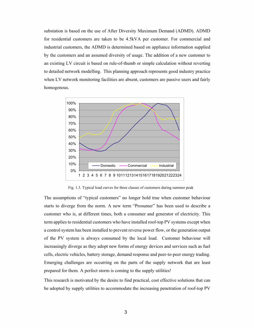
In this environment, planning of LV networks incorporates significant assumptions of

customer homogeneity. JEN estimates customer load consumption during the summer

peak using three daily load curves shown in Figure 1.3: residential, commercial and

industrial. Aggregation of customer loads to upstream supply circuit and distribution

Fig. 1.2. Augmentation expenditure of JEN

Fig. 1.1. A residential roof-top PV installation

3

substation is based on the use of After Diversity Maximum Demand (ADMD). ADMD

for residential customers are taken to be 4.5kVA per customer. For commercial and

industrial customers, the ADMD is determined based on appliance information supplied

by the customers and an assumed diversity of usage. The addition of a new customer to

an existing LV circuit is based on rule-of-thumb or simple calculation without reverting

to detailed network modelling. This planning approach represents good industry practice

when LV network monitoring facilities are absent, customers are passive users and fairly

homogenous.

The assumptions of “typical customers” no longer hold true when customer behaviour

starts to diverge from the norm. A new term “Prosumer” has been used to describe a

customer who is, at different times, both a consumer and generator of electricity. This

term applies to residential customers who have installed roof-top PV systems except when

a control system has been installed to prevent reverse power flow, or the generation output

of the PV system is always consumed by the local load. Customer behaviour will

increasingly diverge as they adopt new forms of energy devices and services such as fuel

cells, electric vehicles, battery storage, demand response and peer-to-peer energy trading.

Emerging challenges are occurring on the parts of the supply network that are least

prepared for them. A perfect storm is coming to the supply utilities!

This research is motivated by the desire to find practical, cost effective solutions that can

be adopted by supply utilities to accommodate the increasing penetration of roof-top PV

Fig. 1.3. Typical load curves for three classes of customers during summer peak

0%

10%

20%

30%

40%

50%

60%

70%

80%

90%

100%

1 2 3 4 5 6 7 8 9 101112131415161718192021222324

Domestic Commercial Industrial

4

systems, and in this way preserve or even increase the value of the supply network to the

modern-day customers.

Key Objectives

The key objectives of this research are synopsised as follows:

Perform exploratory analysis of voltage quality data collected by smart meters and

develop, on a macro level, insight about steady-state voltage delivery to

customers;

Determine, based on anecdotal evidence and smart meter voltage quality data

analysis, how grid connected residential PV systems contribute to voltage quality

issues;

Develop a Low Voltage network model which can be used to simulate the effect

of PV on steady-state voltage levels. The model shall be accurate enough for

network planning purposes and incorporate data sets that can be reasonably

collected by supply authorities:

o Simplified PV output model based on panel DC rating, inverter AC rating,

panel orientation and environmental parameters collected by public

weather stations;

o 4-wire LV network design comprising single-phase loads connected

between phase and neutral conductors as well as three-phase loads within

a Multiple Earthed Neutral (MEN) system;

o Time series load and generation data collected by smart meters and

Supervisory Control and Data Acquisition (SCADA) system;

o Conventional utility voltage control systems consisting of voltage

regulating schemes acting on transformers with on-load tap changers,

substation switched shunt capacitor banks and line switched shunt

capacitor banks.

o Smart grid voltage control systems consisting of on-load tap changing

distribution transformer, smart PV inverter and battery storage system.

Perform time series load flow simulation studies to obtain LV network voltage

profiles for different network configurations and voltage control system scenarios,

for different PV penetration levels.

5

Make recommendations to supply authorities on changes to their network

planning policies and adoption of smart network technologies in order to increase

the capacity of their LV distribution networks to accommodate the increasing

penetration of PV generation systems.

Design and Methodology

Literature Review

Interest in the behaviour of grid connected PV systems has intensified in recent years due

to the continual decline in system costs making the systems more affordable and the

number of installations has increased considerably. A body of knowledge has been

developed on models that can accurately represent the various components of the PV

systems and how the components interact to produce energy on an annual basis. Models

with higher time resolution have also been developed to model the transient impact on

the supply grid. These models generally require design parameters that can reasonably be

collected for large systems connected to the Medium Voltage or High Voltage grids but

will require significant simplification for small PV systems installed by residential

customers.

The PV models developed have been used in system studies to determine the upper limit

of PV penetration before serious issues arise. Due to the different assumptions of network

characteristics and generally idealised installation conditions, these limits cannot be

readily used by electricity supply companies.

While big data analytics techniques have been applied to many service industries such as

finance and banking, smart meter data analytics is a relatively new research area as mass

rollout of smart meters to residential customers started to occur only around mid 2000s.

This area of research is primarily driven by supply utilities as they have access to the

meter data and are keen to unlock the value of the data to improve planning and

operational performance of their supply networks.

Supply utility voltage control techniques have remained fundamentally the same since

electrification of societies occurred over 100 years ago. This is evidenced by the lack of

research papers published on the topic. With the advance of small generators embedded

in the distribution network, there is renewed research interest on improving utility voltage

control to manage the impact of these small embedded generators. Some large-scale smart

grid demonstration projects in the U.S. and Europe have specifically include the trial of

6

various advanced voltage control schemes to alleviate the impact of embedded generation

on supply voltage quality.

The literature review focuses on scientific research papers on PV characteristics, technical

journals and industry conferences where relevant results of industry research are

disseminated.

Methodology

Smart meter voltage quality data (supplemented by energy consumption data where

required) of approximately 100,000 residential customers over a 1-week period are

collected for exploratory data analysis. The majority of these customers have a net

metering scheme where the energy meter records the net consumption/generation over

each 30-minute integration time interval. The exploratory data analysis yields macro-

level insight on the existing voltage quality delivered to utility customers including

customers who have installed grid connected PV generation systems.

Literature review is conducted to identify the appropriate PV generation output model

that can be used in system studies. Simplification of the PV output model is attempted to

reduce the number of model parameters in order to improve the practicality of the model

for use in distribution system studies.

Accuracy of the simplified PV output model is tested on a number of PV customers who

have gross metering schemes where the generation output and load consumption are

metered separately.

To test the effect of various voltage control schemes on managing voltage issues caused

by embedded PV generation, parameters of an actual LV distribution circuit are

determined and then set up in a network model. This approach is preferred by supply

utilities over the use of “typical” circuits and is becoming increasingly feasible with the

mass rollout of smart meters. The circuit model is set up in OpenDSSTM where load flow

simulations are run. MATLAB© interfaces with OpenDSSTM and is used to vary the PV

penetration level and voltage control schemes, and to analyse the load flow results.

Based on the modelled results, recommendations are made for supply authorities on

changes to their network planning policies and adoption of smart network technologies

that will increase the capacity of their LV distribution networks to accommodate the

increasing penetration of PV generation systems.

7

Research Significance

The installation of grid connected renewable generation systems, in particular PV

systems, is an unstoppable trend worldwide. For the small grid connected PV systems,

government regulators and customers are demanding a streamlined connection process

which generally translates into automatic connection policy for systems under a certain

kVA limit. Even small systems can cause localised voltage issues and when in aggregate,

can affect the upstream supply network. Voltage quality non-compliance has high societal

costs as this affects the performance, energy efficiency and longevity of customer

electrical equipment. As LV networks are generally not observable to utility engineers,

utility engineers tend to apply conservative limits to enforce their responsibility for

voltage quality. This limits the amount of small PV generators that can be automatically

connected to the supply network. When the limit is reached, utilities will need to assess

each proposed connection on a case-by-case basis, generally via background

measurement and modelling. The lack of an appropriate PV generation model and an

accurate LV model again hinders the effectiveness and efficiency of this assessment

process.

This research, enabled by the availability of smart meter data, provides recommendations

on the establishment of accurate network models and improvements to existing

operational practices (voltage control schemes and phase connection of PV generation)

so as to increase the capacity of the LV network to host embedded PV generation, before

resorting to significant investment in network augmentation and smart grid technologies.

Original Contribution

Electricity supply utilities worldwide are transforming themselves from an infrastructure

provider (“poles and wires” business) to an enabler of various energy services. This

transformation is driven by customer preference and is crucial to the future survival of

the supply utilities. Pivotal in this transformation process is the development of a

customer focused culture.

This research is motivated by the desire to find practical, cost effective solutions that can

be adopted by supply utilities to accommodate the increasing penetration of customer

roof-top PV systems, and in this way preserve or even increase the value of the supply

network to the modern-day customers. Industry research has been mostly focused on the

development of smart grid technologies as mitigating measures, which generally require

8

significant additional grid investment. While transforming the supply grid performance

by investing in smart grid technologies is unavoidable, customers are already financially

burdened by the transition to a renewable energy future caused by initiatives such as feed-

in tariffs 1 . A prioritised approach of improving existing operational practices and

implementation of smart grid technologies will help to spread the additional investment

cost over a longer time horizon, improve customer service and reduce the risk of customer

defection (leaving the grid).

The research takes an insider view of the supply utility organisation (enabled by this

researcher’s many years of experience working for supply utilities), provides insight of

network planning and voltage control criteria, identifies the challenges caused by grid

connected PV systems, and recommends practical approaches that can be taken to

increase the hosting capacity of the supply network. This end-to-end supply utility focus

is original, and provides significant value to a supply utility on the path of transformation

to a customer-focused energy service provider of the future.

The research is enabled by the availability of residential smart meter data. The mass

rollout of smart meters to residential customers is a recent development and is still on-

going in many parts of the world. Insight on smart meter data developed in the research,

while specific to the network being studied, will be a useful reference for other

distribution networks and demonstrate the value of smart meter data to network service

providers.

Thesis Organisation

This thesis comprises of seven chapters and is organised as follows:

Chapter 1: covers a brief introduction of the key objectives, motivations and

methodologies of the research, while providing insight into the research

significance in the discipline of electrical engineering.

Chapter 2: presents a comprehensive literature review of smart meter data

analytics, impact assessment of grid connected renewable generation systems, PV

generation modelling and options for mitigating the impact of grid connected

renewable generation systems.

1 Feed-in tariffs increase the cost of each unit of electricity, resulting in higher electricity prices to customers who have no access to the feed-in tariffs i.e. those who have not installed a PV system

9

Chapter 3: describes the insight developed by performing exploratory analysis of

smart meter voltage quality data. It highlights the usefulness and limitations of

existing smart meter data and makes recommendations on how the data can be

improved to increase its usefulness.

Chapter 4: develops a PV generation model and demonstrates its use in practical

electricity distribution network applications.

Chapter 5: describes the development of a network model for a real distribution

circuit that has eight residential customers, two of which have grid connected roof-

top PV systems.

Chapter 6: analyses the results of load flow studies performed on the network

model under different network scenarios and voltage control strategies, and

provides recommendations to supply utilities.

Chapter 7: summarises the work in chapters 1-6 and provides recommendations

for future research studies.

Summary

This chapter has introduced the drivers which lead to the significant development of roof-

top residential PV systems. The challenge to supply utilities arising from the development

is outlined and the strategic objectives for supply utilities to allow connection of these

embedded generation system are described. Attention is brought to the motivation and

scope of this research, and the main contributions listed. Finally, the thesis structure and

main contents of each chapter are briefly outlined.

10

Chapter 2 - Literature Review

Overview

This chapter presents a comprehensive review of the research in voltage quality impact

caused by embedded generation, in particular, residential roof-top PV installations

connected to the LV networks and the potential mitigating measures that can be applied.

Section 2.2 provides some background to the quality of supply in the existing LV

networks. Section 2.3 examines the impact of grid connected PV systems. Section 2.4

reviews the use of smart meter data to improve the visibility of the LV networks. Section

2.5 reviews network modelling techniques that are used to quantify the impact of PV

systems on LV network performance. Section 2.6 addresses methods which have been

used to improve the hosting capacity of LV networks for PV generators. Finally, based

on the literature survey, Section 2.7 summarises the key issues identified.

Quality of Supply in the Low Voltage Networks

There is renewed interest in the quality of supply in the LV networks due to increasing

connection of residential PV systems and other emerging customer technologies (such as

electric vehicles and energy storage systems). While standards for quality of supply in

LV networks have been established (e.g. AS/NZS 61000.3. series), due to the high cost

of providing permanent power quality monitoring at every customer connection point

compliance measurement is generally carried out on customer complaints or as one-off

statistical programs. Since year 2000, the Power Quality Centre of the University of

Wollongong, Australia, has been conducting an annual long-term national power quality

survey involving many electricity distribution companies [2]. The survey focuses on the

power quality data of steady-state voltage, unbalance, harmonics and sags/swells. It is

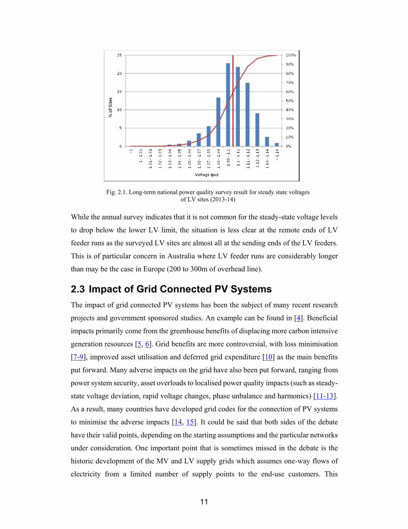
noteworthy that the annual survey has consistently found some 25% to 30% of LV sites

record 95th percentile steady-state voltage levels which are above the upper LV limit

(230V + 10%), predominately during the light load periods (Figure 2.1). High voltage

phenomena during low load periods have also been reported in other countries e.g. the

U.K. [3].

11

While the annual survey indicates that it is not common for the steady-state voltage levels

to drop below the lower LV limit, the situation is less clear at the remote ends of LV

feeder runs as the surveyed LV sites are almost all at the sending ends of the LV feeders.

This is of particular concern in Australia where LV feeder runs are considerably longer

than may be the case in Europe (200 to 300m of overhead line).

Impact of Grid Connected PV Systems

The impact of grid connected PV systems has been the subject of many recent research

projects and government sponsored studies. An example can be found in [4]. Beneficial

impacts primarily come from the greenhouse benefits of displacing more carbon intensive

generation resources [5, 6]. Grid benefits are more controversial, with loss minimisation

[7-9], improved asset utilisation and deferred grid expenditure [10] as the main benefits

put forward. Many adverse impacts on the grid have also been put forward, ranging from

power system security, asset overloads to localised power quality impacts (such as steady-

state voltage deviation, rapid voltage changes, phase unbalance and harmonics) [11-13].

As a result, many countries have developed grid codes for the connection of PV systems

to minimise the adverse impacts [14, 15]. It could be said that both sides of the debate

have their valid points, depending on the starting assumptions and the particular networks

under consideration. One important point that is sometimes missed in the debate is the

historic development of the MV and LV supply grids which assumes one-way flows of

electricity from a limited number of supply points to the end-use customers. This

Fig. 2.1. Long-term national power quality survey result for steady state voltages of LV sites (2013-14)

12

assumption is embedded in network planning philosophies, network design criteria,

control settings as well as equipment deployed. This situation is particularly acute in the

LV networks where the lack of investment means the networks lack observability and

incomplete data capture and record keeping means rules of thumbs are used extensively.

A complete re-think and re-design of the grid is required to accommodate the increasing

level of embedded PV generation.

Voltage Quality Data from Smart Meters

A recent development which comes to the aid of utility engineers is the deployment of

smart meters to residential customers. Smart meters have two important functions:

Electricity tariff function to capture the demand and energy usage of customers. The

electricity tariff function is enhanced by the ability to record usage over pre-defined

time intervals (such as every 15 or 30 minutes) allowing customers to be charged

based on time-of-use tariffs aligning to the real-time cost for the production and

transmission of electricity [16].

Network monitoring functionality to capture network parameters such as voltages,

currents, power factor and supply status.

Equipped with two-way communication capability, smart meters allow customers to

make informed decisions on when and how they consume electricity based on real-time

price signals. They also allow utilities to monitor the quality of supply they are delivering

to their customers at their points of connection, allowing proactive management of

compliance.

Smart meter rollout programs to residential and small commercial/industrial customers

have been reported in a number of countries. In Europe, smart meter rollout programs

have been mandated in fourteen countries [17]. In the state of Victoria, Australia,

government mandated a distributor-led rollout of smart meters to 2.8 million customers

consuming less than 160MWh per annum. The program, known as Advanced Metering

Infrastructure (AMI) program, started in late 2009 and was practically completed by

middle of 2014.

A number of research articles have reported the use of smart meter data to aid in the

management of supply network and the grid connected PV systems. One of the challenges

brought about by smart meters is the sheer volume of data being collected and the time

varying nature of the data. Big data analytics is increasingly applied to derive useful

13

information from the voluminous smart meter data. In [18] data clustering technique is

used to derive a set of MV customer load profile. In [19] data clustering technique is used

on half-hourly smart meter data to better understand how residential customers use

their energy and their effect on the LV networks. In [20] a novel sublinear algorithm uses

a small portion of the smart meter load data to characterize the electricity usage

distributions of different set of users and allows utilities to offer differentiated user

services based on usage patterns.

Ideas on the use of power quality information captured by AMI and smart meters to

optimise the operational efficiencies of LV networks are reported in [21]. Implementation

of innovative initiatives have been reported in a number of simulations and trials. [22]

reports the use of voltages and currents for the calculation of line impedance between

supply nodes. [23, 24] propose methodologies to determine the consumer phase

connection using voltage information from customer smart meters. [25] uses smart meter

instantaneous power measurements to derive phase unbalance on the LV distribution

circuit and proposes the use of static transfer switches to dynamically switch houses from

the initial connected phase to another, to reduce voltage unbalance. With smart meter

recording voltage quality data such as voltage, current and power factor at the customer

connection points, visibility of the LV networks has dramatically improved and this paves

the way for better management of grid connected PV systems.

Network Modelling Techniques

A number of studies have attempted to quantify the upper limits of PV penetration before

serious network issues arise. In 2007, the US Department of Energy’s Renewable System

Integration project conducted a literature search and utility engineer survey [11]. The

literature survey reveals that a range of limits have been reported for PV penetration on a

feeder or system level, between 5% and 40%, depending on the characteristics of the

network and the parameters that are found to be limiting. Technical parameters include

fast ramp rate requirement of central generators, reverse power swings on cloud

transients, excessive load tap changer operations, overvoltage at light load conditions and

undervoltage on sudden loss of PV generation. Economic parameters include increased

distribution system losses, increased tie-line flows and increased frequency regulation

costs. Unacceptable flicker emission caused by cloud transients have also been reported

14

[26]. Combination of theoretical modelling techniques and experimental results has been

used to derive the PV impacts and to infer the penetration limits.

A number of key components are required for an accurate network model incorporating

PV systems:

PV generation model - Current research on PV models tends to focus on establishing

the electrical representations of the various components that make up a PV installation

e.g. solar panels, inverter, associated wirings, etc., and determine PV output based on

how these components interact with external factors such as solar irradiance, ambient

temperature and wind speed, while taking into account panel orientation, solar cell

efficiency and electrical losses [27-29]. These complex models provide accurate

output prediction but required extensive data collection effort.

Circuit impedance – in Australia the MV network (typically 11kV or 22kV) is

generally 3-phase 3-wire (R, W, B) construction with 3-phase distribution transformer

(MV/LV) connected in delta on the MV side and star on the LV side. Single-phase

distribution transformers are also used in the rural areas. The MV therefore needs to

be modelled as a three-phase 3-conductor unbalanced network. The LV network

emulating from the MV/LV distribution transformer is generally 3-phase 4-wire (R,

W, B and N), un-transposed, with customers connected between phase and neutral. A

Multiple Earthed Neutral (MEN) system is implemented where the neutral conductor

is earthed at customer points of connection as well as at the LV star point of the supply

distribution transformer. The LV needs to model both the neutral conductor and the

earth connection as the loads are inherently unbalanced (due to 1-phase customer

connections) so currents will flow in both the neutral conductor and earth, leading to

voltages appearing on the neutral conductor [30-32]. Carson’s equations can be used

to derive the self and mutual impedances of overhead and underground conductors

taking into account the return path of current through ground and phase asymmetry

(un-transposed phase conductors) [33].

Customer phase connectivity – it is important that phase connection of single-phase

LV customers is accurately modelled, as the load/generation balance on each phase

plays a significant role on the voltage profile of the LV distribution circuit [34].

Customer load profile – as discussed above, detailed modelling of loads and

generation on each phase is required to accurately determine the voltage profile on

the LV distribution circuit.

15

To master the vast amount of network and customer data requires efficient network

analysis techniques. [35] describes an advanced analysis tool for the assessment of

clustered rooftop solar PV impacts. From the large volume of real-time network data

collected from monitoring systems or smart meters, the tool is able to intelligently decide

which part of the data would be effective for analysis of solar PV impacts, using data

mining techniques to discover hidden patterns and Symbolic Aggregate Approximation

(SAX) to reduce the dimensionality of the database. With both loads and PV generations

both stochastic in nature, probabilistic load flows are proposed such as Monte Carlo based

techniques [36] and analytical method that combines the cumulant method with the

Cornish–Fisher expansion [37]. Finally, to reduce the effort of carrying out assessment

on a large number of LV networks diverse in characteristics, [38] proposes the

development of representative LV feeders from a large number of LV networks using

clustering algorithms.

Methods to Increase the Hosting Capacity of LV Networks for PV Generators

For small grid connected residential PV systems, adverse impacts on the grid are

primarily caused by steady-state voltage change and phase voltage unbalance. Many

research papers have looked at overcoming localised voltage rise caused by embedded

generators. The methods fall into three main categories:

Improve existing voltage regulation schemes – Many electric utilities rely on voltage

regulation schemes on the MV network to deliver the appropriate supply voltage to

their LV customers. Figure 2.2 shows the typical voltage regulation schemes found in

the electricity supply system in Australia.

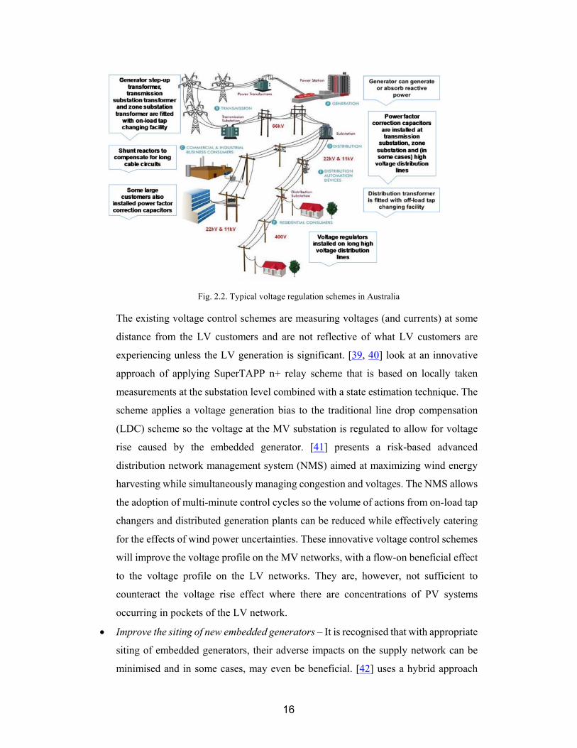
16

The existing voltage control schemes are measuring voltages (and currents) at some

distance from the LV customers and are not reflective of what LV customers are

experiencing unless the LV generation is significant. [39, 40] look at an innovative

approach of applying SuperTAPP n+ relay scheme that is based on locally taken

measurements at the substation level combined with a state estimation technique. The

scheme applies a voltage generation bias to the traditional line drop compensation

(LDC) scheme so the voltage at the MV substation is regulated to allow for voltage

rise caused by the embedded generator. [41] presents a risk-based advanced

distribution network management system (NMS) aimed at maximizing wind energy

harvesting while simultaneously managing congestion and voltages. The NMS allows

the adoption of multi-minute control cycles so the volume of actions from on-load tap

changers and distributed generation plants can be reduced while effectively catering

for the effects of wind power uncertainties. These innovative voltage control schemes

will improve the voltage profile on the MV networks, with a flow-on beneficial effect

to the voltage profile on the LV networks. They are, however, not sufficient to

counteract the voltage rise effect where there are concentrations of PV systems

occurring in pockets of the LV network.

Improve the siting of new embedded generators – It is recognised that with appropriate

siting of embedded generators, their adverse impacts on the supply network can be

minimised and in some cases, may even be beneficial. [42] uses a hybrid approach

Fig. 2.2. Typical voltage regulation schemes in Australia

17

combining Generic Algorithms and Optimal Power Flow to determine locations

where embedded generator connections will minimise capacity augmentation cost and

network losses, based on regulatory incentives in U.K.. However, the methodology is

only applicable to embedded generators connected at MV or above, and the

assessments are made assuming the traditional worst case scenario of maximum

embedded generator output at minimum load. A refined approach using Monte Carlo

simulation to acquire solar radiations, ambient temperatures, load demands and

substation voltages in Optimal Power Flow is presented in [43]. For small PV systems

connected to the LV network, siting of the generators can be improved by switching

from one connected phase to another using static transfer switches as proposed in

[25].

Apply smart grid technologies – This is the area where significant research activity is

occurring. Research directions can be grouped into a number of categories:

o Component approach: Minimise voltage rise and voltage unbalance caused by

excessive PV generation using smart control schemes in the grid connected

PV inverters (active power and/or reactive power control [44-48]), by

installing single-phase switchable LV capacitors [49, 50], by absorbing excess

generation (storage battery [51], other household loads such as water heating,

electric vehicle charging [52]), by the use of distribution on-load tap changing

transformer [53-55], by the use of electronic LV regulator [56], or a

combination of the above [57, 58].

o System approach: Minimise voltage rise by coordinated control at the system

level. [41, 59] describes a distribution Network Management System (NMS)

platform driven by an AC Optimal Power Flow (OPF) engine. The NMS aims

to manage network voltages and congestion (thermal overloads) by

coordinating the control of on-load tap changers, distributed generation

reactive power and curtailment (as last resort). [60] describes an overarching

control area solution, called the Grand Unified Scheme (GUS), which

coordinates the actions of enhanced automatic voltage control scheme,

electrical energy storage, real-time thermal rating and remote terminal units.

Key Issues Identified

Following the comprehensive literature review performed in this chapter, the following

key issues were identified:

18

While the adverse impacts of grid connected PV generators are well established, the

extent of the problem is only known with certainty for locations where actual

measurements have been carried out. Simulations using generalised network models

may provide good indications for formulating high level strategy but are found

lacking in practical applications.

We start to see voltage quality data from smart meters being considered for use in

voltage control schemes. There are, however, limited discussions on the use of smart

meter data to improve the accuracy of LV network data and how the data can be used

in setting up accurate network models for simulation studies.

There is little attention given to the existing voltage quality situation in distribution

networks. Many Australian distribution networks are delivering voltages that are

biased towards the high side so little headroom is left for voltage rise caused by

embedded PV generators. This high voltage bias needs to be fixed and mediated in

conjunction with other approaches to increase the hosting capacity of PV generators.

A lot of attention has been given to the use of smart grid technologies to mitigate the

adverse impact of PV generation but not enough attention is given to improving

existing network planning standards and operating procedures. The investment in

smart grid technologies will generally drive up network costs, at a time when

customers are already financially burdened by government initiatives of moving to a

renewable energy future.

Lastly, it is important that a prioritised approach is taken to tackle the impact of PV

generation so the most cost effective solutions are selected for implementation to suit

the particular characteristics of the distribution network under consideration.

Summary

This chapter has presented a comprehensive literature review of voltage quality issues

caused by PV generation embedded in the distribution network, in particular, the low

voltage network. The availability of smart meter data has enabled a new approach where

the impact of embedded PV generation can be visualised and modelled in network studies.

Various methods to increase the hosting capacity of LV networks for PV generators are

reviewed. Finally, key issues pertaining to current research on PV hosting capacity arising

from the literature review are highlighted.

19

Chapter 3 - Exploratory Analysis

of Smart Meter Voltage Quality

Data

This chapter is based on the following publication:

P.K.C. Wong, R.A. Barr and A. Kalam, “Using smart meter data to improve quality of

voltage delivery in public electricity distribution networks”, Saudi Arabia Smart Grid

Conference, 2012.

Overview

This chapter reports on the insight developed from exploratory analysis of smart meter

voltage quality data. Section 3.2 describes the smart meter rollout program in the state of

Victoria, Australia. Section 3.3 describes the form of the voltage quality data. Results of

exploratory analysis of undervoltage and overvoltage events captured by smart meters are

given in Section 3.4 and 3.5. Section 3.6 focuses on possible solutions to the voltage

issues by analysis that links the smart meter sites to the upstream supply substations.

Section 3.7 presents the case that smart meter data is a form of Big Data that will require

efficient data analytic tools and platforms. Finally, Section 3.8 summarises the insight

developed by performing exploratory analysis of smart meter voltage quality data,

highlights the usefulness and limitations of existing smart meter data and makes

recommendations on how the data can be improved to increase their usefulness.

Smart Meter Rollout Program

Since 2009, the five electricity distribution companies in the state of Victoria, Australia,

have been rolling out smart meters in a program mandated by the state government.

Known as the Advanced Metering Infrastructure (AMI) program, it was completed by

middle of 2014. The mandated program covered all customers consuming under

160MWh per annum, essentially all residential customers, small commercial and small

industrial enterprises. The smart meters are linked by two-way communication network

to a central back office system (Figure 3.1). Apart from 30-minute energy consumption,

the meters also monitor steady-state voltage quality.

20

Forms of Smart Meter Voltage Quality Data

The AMI communication technology utilised by JEN is a mesh radio network between

the AMI meters and the meter access points. The minimum functional specification [61]

of the smart meter program requires AMI meters to be capable of monitoring the supply

voltage and to generate overvoltage and undervoltage alarms when the set thresholds are

exceeded. The function is implemented locally in the smart meters and transmitted to the

central Network Management System as events. In essence a "report by exception"

methodology has been adopted for voltage quality events to better utilise the limited

bandwidth of the mesh radio system.

The events consist of information such as meter identification, event date, start time (for

start events), end time (for stop events), average voltage, maximum (minimum) voltage,

supply address etc. The events can be downloaded from the Network Management

System as Comma-Separated Values (CSV) files. An example of a CSV file containing

voltage events is shown in Figure 3.2 below.

Fig. 3.1. Advanced Metering Infrastructure installed by Jemena Electricity Networks

Fig. 3.2. Example of event list for overvoltage events

21

The undervoltage and overvoltage thresholds are set in accordance with the Victorian

Electricity Distribution Code [62]:

• Undervoltage set point is 216V (230V - 6%);

• Overvoltage set point is 253V (230V + 10%).

To avoid creation of excessive events when the voltage hovers around the threshold

values, a hysteresis setting of 2% (4.8V) is applied. A persistence time is also applied to

avoid reporting on momentary excursions outside limits and is set at 180 seconds. A

diagrammatic representation of the parameters associated with a voltage quality event is

shown in Figure 3.3.

The analysis of smart meter voltage quality events presents a number of challenges.

Firstly, the large volume of data requires efficient data analysis techniques. Secondly, the

events are "snapshots" of voltage delivered to customers (when the supply thresholds are

exceeded) and do not explicitly provide a time series data of voltage delivery. Thirdly, as

the smart meters are not power quality meters designed to AS/NZS61000.4.30 [63], the

events captured can only be treated as indicative and not be used for strict compliance

purpose.

Exploratory Analysis of Smart Meter Voltage Quality Data

Data Set

Overvoltage and undervoltage events reported by 100,000 smart meters, over a 6-day

period in summer 2012, were downloaded from the Network Management System as

Sta

rt E

ve

nt

En

d E

ve

nt

persistence

Event Duration

Sta

rt P

ea

k V

olta

ge

Sta

rt A

ve

rag

e V

olta

ge

persistence

En

d P

ea

k V

olta

ge

En

d A

ve

rag

e V

olta

ge

Hyste

resis

Time

Voltage

Threshold

Customer Supply Voltage

Event Time

Fig. 3.3. Parameters associated with a voltage quality event

22

CSV files. A total of 15,180 undervoltage events and 38,238 overvoltage events were

captured over the 6-day period. Other database extracts include network loading data from

Supervisory Control and Data Acquisition (SCADA) system, network topology snapshots

from Geographical Information System (GIS), residential PV installation data from GIS,

meter reference data from SAP, and ambient temperature information from the Bureau of

Meteorology. Microsoft Excel is used as the software tool to ‘slice and dice’ the data in

a number of ways to answer questions such as

How many overvoltage and undervoltage events occur in the 6-day period?

Is there any relationship between the number of voltage events and

o ambient temperature?

o electricity usage?

How many customer sites are affected?

Are the sites consistently producing overvoltage and undervoltage events over the 6-

day period?

Are there sites that produce both overvoltage and undervoltage events?

At what times of day do the voltage events occur?

How long do these voltage events last?

What are the trigger voltages for these events?

What are the extreme voltages experienced during these events?

From an electrical connectivity perspective, are these customers supplied from the

same distribution circuits, same distribution substations or same zone (primary)

substations?

Results of the exploratory data analysis are detailed in the next section.

Analysis of Undervoltage Events

Before analysis is carried out, the undervoltage event data is cleansed to remove outliers

caused by network faults such as supply interruptions and brown-outs (where voltage

goes down to abnormally low level due to the loss of one phase of the high voltage

supply), and short duration undervoltages that have marginal effect on equipment thermal

performance. After data cleansing, a total of 15,180 undervoltage events were captured

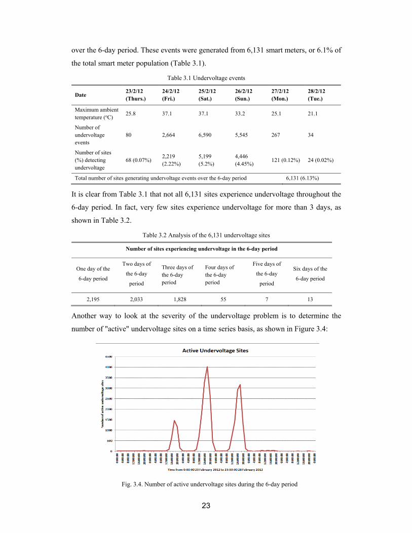
23

over the 6-day period. These events were generated from 6,131 smart meters, or 6.1% of

the total smart meter population (Table 3.1).

Table 3.1 Undervoltage events

Date 23/2/12 (Thurs.)

24/2/12 (Fri.)

25/2/12 (Sat.)

26/2/12 (Sun.)

27/2/12 (Mon.)

28/2/12 (Tue.)

Maximum ambient temperature (oC)

25.8 37.1 37.1 33.2 25.1 21.1

Number of undervoltage events

80 2,664 6,590 5,545 267 34

Number of sites (%) detecting undervoltage

68 (0.07%) 2,219 (2.22%)

5,199 (5.2%)

4,446 (4.45%)

121 (0.12%) 24 (0.02%)

Total number of sites generating undervoltage events over the 6-day period 6,131 (6.13%)

It is clear from Table 3.1 that not all 6,131 sites experience undervoltage throughout the

6-day period. In fact, very few sites experience undervoltage for more than 3 days, as

shown in Table 3.2.

Table 3.2 Analysis of the 6,131 undervoltage sites

Number of sites experiencing undervoltage in the 6-day period

One day of the

6-day period

Two days of

the 6-day

period

Three days of the 6-day period

Four days of the 6-day period

Five days of

the 6-day

period

Six days of the

6-day period

2,195 2,033 1,828 55 7 13

Another way to look at the severity of the undervoltage problem is to determine the

number of "active" undervoltage sites on a time series basis, as shown in Figure 3.4:

Fig. 3.4. Number of active undervoltage sites during the 6-day period

24

Correlation of undervoltage events with ambient temperature

It is observed that the number of undervoltage events exhibits strong correlation with

ambient temperature (Figure 3.5). Undervoltage events are virtually non-existent when

daily maximum ambient temperature is below mid 20s, but the number of events rises

rapidly when the maximum ambient temperature reaches the mid 30s. This indicates that

undervoltage events are triggered by the use of space cooling equipment during high

ambient temperature, primarily refrigerated air conditioning. The increase in loading on

the distribution equipment and circuits causes increases in voltage drop, with resultant

undervoltage experienced by customers especially near the end of low voltage

distribution circuits. The data indicates that a significant number of customers (6%) have

experienced some instances of undervoltage during the three consecutive hot days,

peaking at 5.2% of customers on 25th February.

Fig. 3.5. Number of undervoltage events versus maximum daily ambient temperature

25

Start Times of Undervoltage Events

The majority of undervoltage events commenced between noon to 8pm at night, generally

coinciding with heavy electricity usage (Figure 3.6).

Duration of Undervoltage Events

One key indicator of the severity of an undervoltage event is its duration. Figure 3.7 shows

the number of undervoltage events and their duration. It is observed that the longest

undervoltage event lasted nearly 15 hours. Most of the undervoltage events, however,

lasted between half an hour to 8 hours.

Fig. 3.7. Number of undervoltage events versus duration (minutes)

Fig. 3.6. Number of undervoltage events versus start times

26

Residual Voltage

The event records the lowest voltage during the duration of the undervoltage event. It

does not mean the voltage stays at this low level during the whole event. The lowest

voltage recorded varied from 161V to 216V. It can be seen from Figure 3.8 below that

majority of the undervoltage events are just marginally below the regulatory threshold

(230V-6% or 216V). From a detailed investigative work perspective, the events with

much lower residual voltage should be given priority.

Analysis of Overvoltage Events

It is observed that there are a lot more overvoltage events generated in a day compared

with undervoltage events. To explore the relationship between undervoltage and

overvoltage events, the same 6-day period is analysed. A total of 38,238 overvoltage

events were generated over the 6-day period. These events were generated from 12,251

smart meters, or 12.3% of the total smart meter population. While a site could experience

multiple overvoltage events in the same 24-hour period, most sites experienced only one

overvoltage event in each 24-hour period (Table 3.3).

Fig. 3.8. Minimum voltage of undervoltage events

27

Table 3.3 Overvoltage events

Date 23/2/12 (Thurs.)

24/2/12 (Fri.)

25/2/12 (Sat.)

26/2/12 (Sun.)

27/2/12 (Mon.)

28/2/12 (Tue.)

Number of overvoltage events 8,407 6,129 4,942 6,249 6,733 5,778

Number (%) of sites giving overvoltage events

6,294 (6.29%)

4,724 (4.72%)

3,957 (3.96%)

4,620 (4.62%)

4,733 (4.73%) 3,378 (3.38%)

Total number of sites giving overvoltage events over the 6-day period 12,251 (12.3%)

It is clear from Table 3.3 that the 12,251 sites only give rise to overvoltage events

occasionally during the 6-day period. In fact, very few sites give rise to overvoltage event

throughout the period, as show in Table 3.4.

Table 3.4 Analysis of the 6,131 overvoltage sites

Number of sites experiencing overvoltage in the 6-day period

One day of the 6-day period

Two days of the 6-day period

Three days of the 6-day period

Four days of the 6-day period

Five days of the 6-day period

Six days of the 6-day period

5,192 2,803 2,465 1,242 549 300

Another way to look at the severity of the overvoltage problem is to determine the number

of "active" overvoltage sites on a time series basis, as shown in Figure 3.9.

Fig. 3.9. Number of active overvoltage sites during the 6-day period

28

Figure 3.9 indicates that there are significant overvoltage problems within the electricity

network, with the number of active overvoltage sites in the range of 6,000 or more during

a normal temperature day. Even during high ambient temperature days when electricity

usage has increased, there are still a minimum of 1,000 sites experiencing overvoltage at

any time of the day.

Correlation of overvoltage events with ambient temperature

Unlike undervoltage events, it is observed that the number of overvoltage events do not

show strong correlation with ambient temperature (Figure 3.10).

This is expected as overvoltage generally occurs at light load periods when the voltage

drop across the distribution circuit is at its minimum. As Melbourne summers tend to

have high temperatures during the day and cooler temperatures at night, use of air

conditioners during the light load period (i.e. at night) is infrequent unless there are

consecutive hot days. One would therefore expect that overvoltage would still be

prevalent at light load period even during hot days.

Start times of overvoltage events

By far the most common start times for overvoltage events are 10pm to 2am (Figure 3.11).

This coincides with lower electricity usage.

Fig. 3.10. Percentage of sites giving overvoltage events versus maximum daily ambient temperature

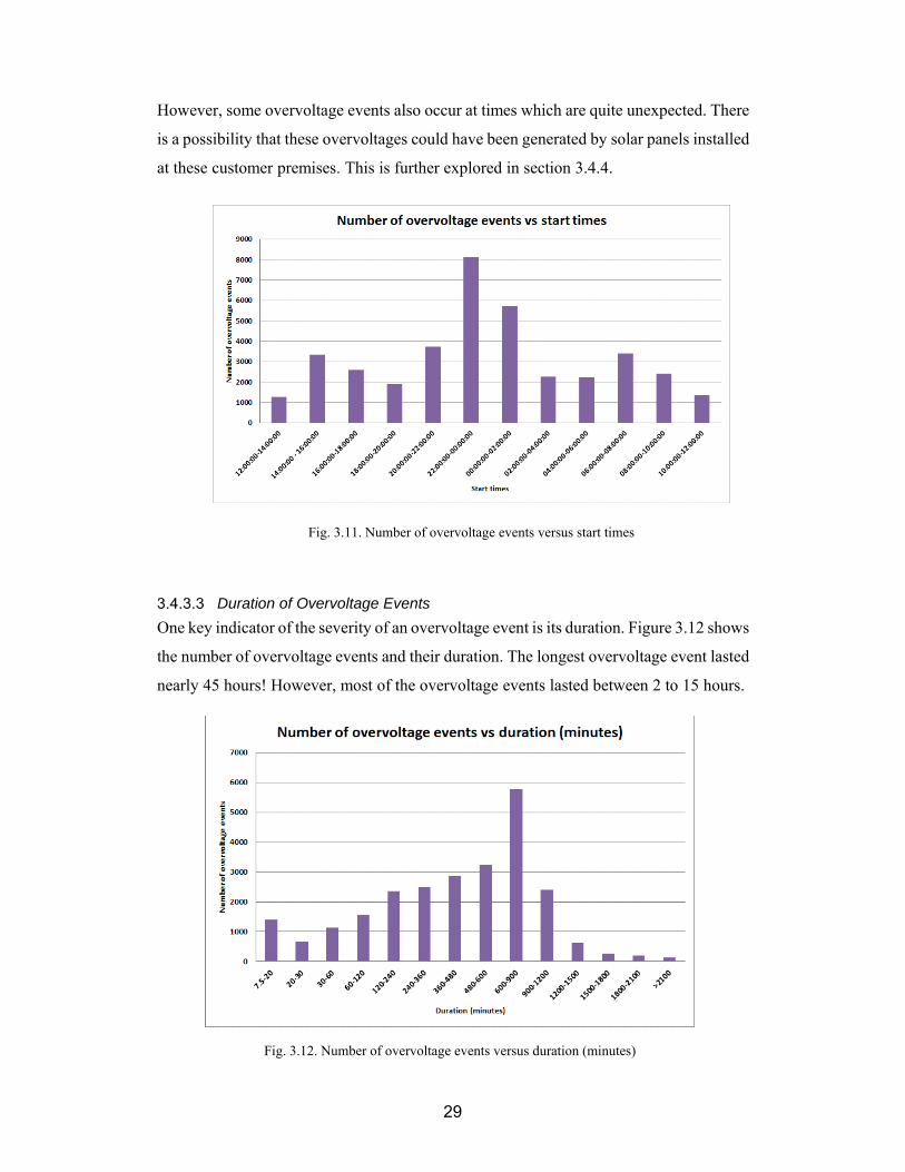
29

However, some overvoltage events also occur at times which are quite unexpected. There

is a possibility that these overvoltages could have been generated by solar panels installed

at these customer premises. This is further explored in section 3.4.4.

Duration of Overvoltage Events

One key indicator of the severity of an overvoltage event is its duration. Figure 3.12 shows

the number of overvoltage events and their duration. The longest overvoltage event lasted

nearly 45 hours! However, most of the overvoltage events lasted between 2 to 15 hours.

Fig. 3.12. Number of overvoltage events versus duration (minutes)

Fig. 3.11. Number of overvoltage events versus start times

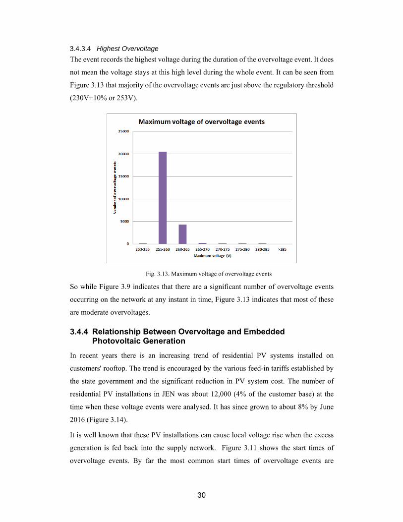
30

Highest Overvoltage

The event records the highest voltage during the duration of the overvoltage event. It does

not mean the voltage stays at this high level during the whole event. It can be seen from

Figure 3.13 that majority of the overvoltage events are just above the regulatory threshold

(230V+10% or 253V).

So while Figure 3.9 indicates that there are a significant number of overvoltage events

occurring on the network at any instant in time, Figure 3.13 indicates that most of these

are moderate overvoltages.

Relationship Between Overvoltage and Embedded Photovoltaic Generation

In recent years there is an increasing trend of residential PV systems installed on

customers' rooftop. The trend is encouraged by the various feed-in tariffs established by

the state government and the significant reduction in PV system cost. The number of

residential PV installations in JEN was about 12,000 (4% of the customer base) at the

time when these voltage events were analysed. It has since grown to about 8% by June

2016 (Figure 3.14).

It is well known that these PV installations can cause local voltage rise when the excess

generation is fed back into the supply network. Figure 3.11 shows the start times of

overvoltage events. By far the most common start times of overvoltage events are

Fig. 3.13. Maximum voltage of overvoltage events

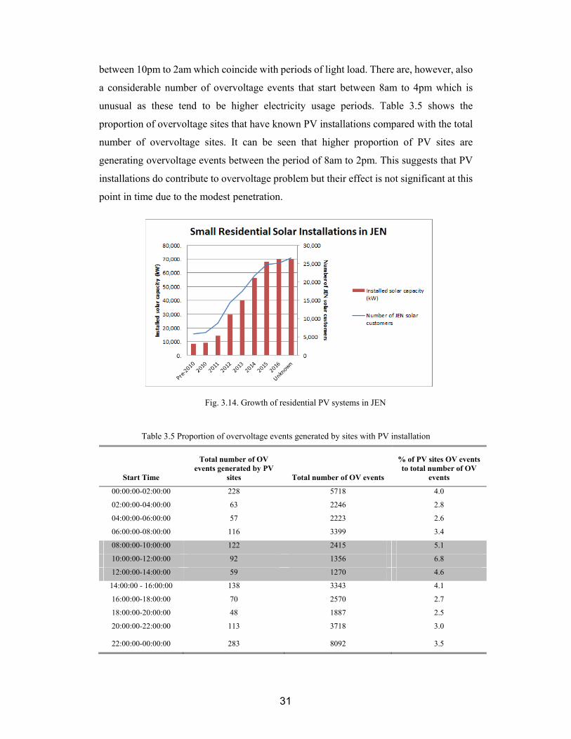
31

between 10pm to 2am which coincide with periods of light load. There are, however, also

a considerable number of overvoltage events that start between 8am to 4pm which is

unusual as these tend to be higher electricity usage periods. Table 3.5 shows the

proportion of overvoltage sites that have known PV installations compared with the total

number of overvoltage sites. It can be seen that higher proportion of PV sites are

generating overvoltage events between the period of 8am to 2pm. This suggests that PV

installations do contribute to overvoltage problem but their effect is not significant at this

point in time due to the modest penetration.

Table 3.5 Proportion of overvoltage events generated by sites with PV installation

Start Time

Total number of OV events generated by PV

sites Total number of OV events

% of PV sites OV events to total number of OV

events

00:00:00-02:00:00 228 5718 4.0

02:00:00-04:00:00 63 2246 2.8

04:00:00-06:00:00 57 2223 2.6

06:00:00-08:00:00 116 3399 3.4

08:00:00-10:00:00 122 2415 5.1

10:00:00-12:00:00 92 1356 6.8

12:00:00-14:00:00 59 1270 4.6

14:00:00 - 16:00:00 138 3343 4.1

16:00:00-18:00:00 70 2570 2.7

18:00:00-20:00:00 48 1887 2.5

20:00:00-22:00:00 113 3718 3.0

22:00:00-00:00:00 283 8092 3.5

Fig. 3.14. Growth of residential PV systems in JEN

32

Relationship Between Voltage Non-compliance and Customer Complaints

Before the era of smart meters, utilities could not continually monitor the quality of the

voltage they deliver to customers due to the high monitoring costs. Most utilities relied

on customer complaints as a trigger to undertake more detailed measurements. For JEN

there were about 120 cases of confirmed voltage complaints in year 2011 attributed to a

number of causes as shown in Figure 3.15. This number of voltage complaints is just not

comparable with what has been revealed by smart meters (15,180 undervoltage and

38,238 overvoltage events in a 6-day period). This indicates that the effect of

undervoltages and overvoltages is generally not apparent to most customers as their

appliances often continue to work under these conditions. The life and performance of

these appliances, however, are affected and this represents the ‘hidden’ cost of voltage

quality non-compliance.

Linking Voltage Quality Events to Supply Substations

For the purpose of voltage regulation, distribution substations are fitted with off-load

transformer tap changing facility. Zone substations are generally fitted with transformer

on-load tap changer controlled by voltage regulating relays. In JEN some zone substations

are regulated at a flat supply voltage while some others have Line Drop Compensation

(LDC) applied.

Fig. 3.15. Analysis of customer voltage complaints

3%

11%

37%

3%

21%

25%

2011 Voltage Complaints

Faults

Flickering Volts

High Volts

Internal

Low Volts

Overload

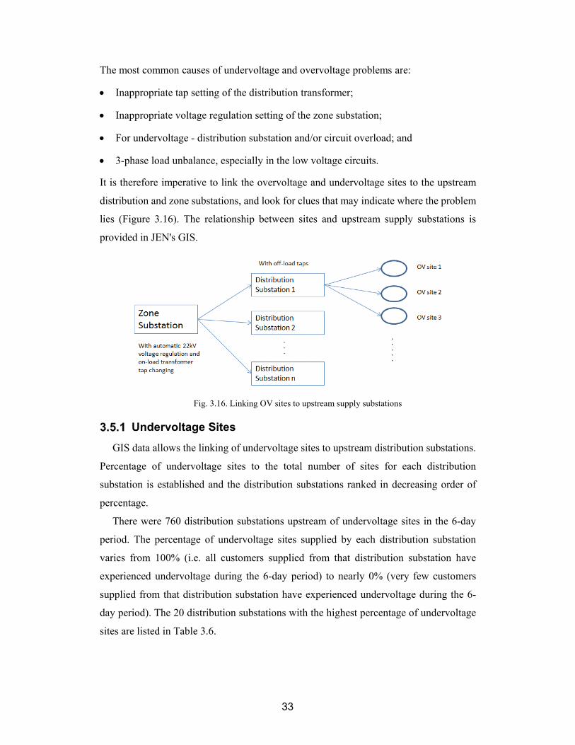
33

The most common causes of undervoltage and overvoltage problems are:

Inappropriate tap setting of the distribution transformer;

Inappropriate voltage regulation setting of the zone substation;

For undervoltage - distribution substation and/or circuit overload; and

3-phase load unbalance, especially in the low voltage circuits.

It is therefore imperative to link the overvoltage and undervoltage sites to the upstream

distribution and zone substations, and look for clues that may indicate where the problem

lies (Figure 3.16). The relationship between sites and upstream supply substations is

provided in JEN's GIS.

Undervoltage Sites

GIS data allows the linking of undervoltage sites to upstream distribution substations.

Percentage of undervoltage sites to the total number of sites for each distribution

substation is established and the distribution substations ranked in decreasing order of

percentage.

There were 760 distribution substations upstream of undervoltage sites in the 6-day

period. The percentage of undervoltage sites supplied by each distribution substation

varies from 100% (i.e. all customers supplied from that distribution substation have

experienced undervoltage during the 6-day period) to nearly 0% (very few customers

supplied from that distribution substation have experienced undervoltage during the 6-

day period). The 20 distribution substations with the highest percentage of undervoltage

sites are listed in Table 3.6.

Fig. 3.16. Linking OV sites to upstream supply substations

34

Table 3.6 20 distribution substations with the highest percentage of undervoltage sites in the 6-day period

Distribution substation Undervoltage sites Total number of sites % of sites with UV events

ST GEORGES 102-MURRAY 62 100 62.0%

STUDLEY-BANKSIA 26 65 40.0%

VALLEY-AUGUSTINE 59 170 34.7%

SEXTON-HALSEY 97 288 33.7%

GOURLAY-SUGAR GUM 21 64 32.8%

LAURIE-PURINUAN 51 165 30.9%

YALLAMBIE-JANICE 36 120 30.0%

BLACK-MC MAHON 31 111 27.9%

PASCOE VALE-SHANKLAND 43 157 27.4%

HART-BOWES 77 282 27.3%

DUFFY-BARRY 64 240 26.7%

FULLARTON-WALTERS 20 78 25.6%

CUDGEWA-BORVA 33 129 25.6%

WARANGA-BLAIR 46 180 25.6%

VICTORY-FOSTERS 51 203 25.1%

MOUSHALL-NOLAN 50 205 24.4%

GRAHAM 138-SYLVIA 48 201 23.9%

BLIBURG-SUNSET 33 141 23.4%

MULBERRY-GONA 45 209 21.5%

GREEN-SPARKFORD 41 193 21.2%

Before taking the decision to change the taps on these distribution transformers, it is

important to check if these distribution substations are affected by inappropriate voltage

regulation settings at the upstream zone substation. One method to establish this

relationship for each zone substation is to determine the percentage of downstream

distribution substations that have experienced undervoltage events. The result for the ten

worst zone substation is tabulated in Table 3.7.

35

Table 3.7 Ten worst zone substations which supply distribution substations with undervoltage events

Zone Sub

Number of distribution substations with undervoltage events

Total number of distribution substations

% of distribution substations with undervoltage events

TT 72 137 52.6%

HB 45 105 42.9%

PV 59 159 37.1%

ES 42 136 30.9%

CS 63 216 29.2%

NH 73 255 28.6%

NT 41 145 28.3%

BY 34 129 26.4%

NS 26 108 24.1%

CN 70 299 23.4%

Overvoltage Sites

GIS data allows the linking of overvoltage sites to upstream distribution substations.

Percentage of overvoltage sites to the total number of sites for each distribution substation

is established and the distribution substations ranked in decreasing order of percentage.

There were 922 distribution substations upstream of overvoltage sites in the 6-day period.

The percentage of overvoltage sites supplied by each distribution substation varies from

100% (i.e. all customers supplied from that distribution substation have experienced

overvoltage during the 6-day period) to nearly 0% (very few customers supplied from

that distribution substation have experienced overvoltage during the 6-day period). The

20 distribution substations with the highest percentage of overvoltage sites are listed in

Table 3.8.

36

Table 3.8 20 distribution substations with the highest percentage of overvoltage sites in the 6-day period

Distribution substation Overvoltage sites Total Number of Sites % of sites with OV events

BARRINGTON LA-P6A 1 1 100.0%

WOOD-NORTHLAND 46 53 86.8%

LOVAT-LONGFORD 41 50 82.0%

BARRY-PASCOE VALE 22 27 81.5%

GRAHAM-ULRICH 123 152 80.9%

AUGUSTA-HUME 23 29 79.3%

STAWELL-CLUNES 54 73 74.0%

TATE-LIVINGSTONE 93 127 73.2%

PAVLEKA-ALLENBY 101 138 73.2%

BLAKE-SESTON 77 113 68.1%

DARLING-WHITE 127 189 67.2%

IRONBARK-RUTHERFORD 88 131 67.2%

WATTLEVALLEY-GOLDEN 80 121 66.1%

LONDON-CUTHBERT 103 156 66.0%

BUSHFIELD-LONGFORD 17 26 65.4%

HUME-PARAMOUNT CO 20 31 64.5%

MOROBE-ALAMEIN 28 44 63.6%

THORPDALE-KYABRAM 40 63 63.5%

CHURCHILL-COONAMAR 40 64 62.5%

JOHNSON-BENAUD 82 135 60.7%

Before taking the decision to change the taps on these distribution transformers, it is

important to check if these distribution substations are affected by inappropriate voltage

regulation settings at the upstream zone substation. One method to establish this

relationship for each zone substation is to determine the percentage of downstream

distribution substations that have experienced overvoltage events. The result for the ten

worst zone substations is tabulated in Table 3.9.

37

Table 3.9 Ten worst zone substations which supply distribution substations with overvoltage events

Zone Sub

Number of distribution substations with overvoltage events

Total number of distribution substations

% of distribution substations with overvoltage events

FF 38 70 54.3%

PV 66 159 41.5%

NS 37 108 34.3%

ES 46 136 33.8%

YTS 34 124 27.4%

P 13 48 27.1%

CN 80 299 26.8%

NH 67 255 26.3%

TT 28 137 20.4%

BD 99 489 20.2%

Sites Experiencing both Overvoltage and Undervoltage

During the 6-day period, 12,251 sites and 6,131 sites experienced overvoltage and

undervoltage events respectively.

There were 88 sites that have experienced both undervoltages and overvoltages. These

sites present a unique problem in that the voltage issues cannot be fixed simply by raising

or lowering the voltage regulation. There are only 4 sites with PV installation in this group

so it appears PV does not contribute to the overvoltage issue.

These 88 sites are linked to 31 distribution substations. The seven worst distribution

substations are shown in Table 3.10.

Table 3.10 Seven worst distribution substations whose customers have experienced both overvoltage and undervoltage events in the 6-day period

Distribution substation Number of sites with both overvoltage and undervoltage

MCCOLL-MALPAS 11

SEPARATION-FULHAM 10

ARTHUR-SEPARATION 9

BLOOMFIELD-ROSAMOND 8

DARLING-WHITE 7

DELAWARE-MENDIP 5

MITCHELL-GILLIES 4

38

Of these 7 distribution substations, Arthur-Separation and Mitchell-Gillies are already

earmarked for capacity upgrade due to confirmed substation overload.

A Big Data Problem

Gartner, a leading information technology research and advisory company, defines "big

data" as having characteristics that can be denoted by three "Vs": Volume, Velocity and

Variety. Voltage quality data is a form of "big data" as it possesses the following

characteristics:

Volume – Voltage quality events generated from smart meters are voluminous. In the

6-day period, there are 15,180 undervoltage and 38,238 overvoltage events.

Velocity - Velocity refers to the speed of data generation and disappearance. A total

of 6,131 customer sites have experienced undervoltage in the 6-day period. However,

not all 6,131 sites experienced undervoltage throughout the six days. Similarly,

12,251 customer sites experienced overvoltage in the 6-day period but few sites gave

rise to overvoltage events throughout the period. In other words, under and

overvoltage conditions are transient in nature and do not form an easily recognisable

pattern.

Variety - Variety refers to the number of disparate databases containing data that must

be processed for enhanced insight and decision making. To allow corrective action to

be taken, the smart meter voltage quality data must be analysed in conjunction with

network connectivity data (stored in spatial database such as GIS), network asset data

(in GIS and/or SAP) and real-time voltage data (in SCADA).

The exploratory data analysis conducted in 3.4 and 3.5 is valuable as it allows insight to

be gained on the specification for the ultimate data analytic tools, the ancillary data

requirement as well as the types of queries to be run on the data sets. Efficient data

analytic tools including in-memory processing databases are required to handle the big

data generated by smart meters.

Summary

The exploratory data analysis reveals the following useful insights:

Strong correlation of undervoltage events with ambient temperature – undervoltage

events are virtually non-existent at ambient temperature below mid 20s, and rising

39

rapidly when ambient temperature reaches the mid 30s. Overvoltage events, on the

other hand, do not show strong correlation with ambient temperature.

The majority of overvoltage events are caused by the existing voltage regulation being

set marginally too high. This existing practice is likely to limit the amount of

embedded generation (such as PV) that can be connected to the supply network. Care

needs to be exercised, however, to ensure that dropping the voltage regulation setting

will not lead to worsening of the undervoltage situation on hot days.

The appropriateness of conventional Line Drop Compensation voltage regulation

schemes. These schemes may need to be reviewed.

Definitive patterns of start times can be observed for undervoltage events. Coupled

with the insight gained from ambient temperature relationship, adaptive voltage

control schemes based on ambient temperature and time of day could be explored to

improve on the undervoltage situation.

Residential photovoltaic installations, modest in its penetration at the time of analysis

(about 4%), is already observed to have a discernible impact on overvoltage

occurrence. The effect will become more significant as the penetration of PV

increases further.

Priority for voltage non-compliance investigation and rectification can be set based

on the level of voltage deviation and time duration as revealed by the smart meter

voltage events.

Clusters of voltage events around particular distribution substations may indicate

inappropriate off-load transformer tap setting.

Clusters of distribution substations around particular zone substations may indicate

inappropriate on-load tap change voltage regulating relay settings.

Customers who experience both overvoltage and undervoltage events may indicate

an upstream asset overload condition.

The exploratory data analysis also exposes the limitation of the existing voltage quality

data from JEN:

Due to the use of hysteresis, an event does not end until the voltage has restored back

to well within the allowable range. The event duration, obtained by the difference

between the start and stop times, is likely to be longer than duration of the voltage

non-compliance.

40

The lack of accurate phase information of customer connection limits the usefulness

of the data analysis.

Voltage profile along the LV distribution circuit cannot be established due to the lack

of time series data of voltage measurements.

Voltage measurements alone are not sufficient to reveal what is occurring in the

supply network that leads to the voltage non-compliance, e.g. phase current unbalance

could be the cause of overvoltages or undervoltages. Time synchronised current and

power factor measurements, at adequate time resolution, will be required to complete

the picture.

Moreover, due to the limitations posed by Microsoft Excel in the size of CSV files that it

can handle and the computational speed, only 6-day of voltage events can be analysed at

one time. Excel is clearly not suitable for big data analytics.

JEN is currently implementing an enhancement to its AMI to enable the collection of time

synchronised voltage, current and power factor measurements at 5-minute intervals. It is

also implementing an in-memory computing platform for data analytics applications

based on SAP® HANA®. A number of applications are planned with the 5-minute AMI

data, including customer connection phase identification and supply impedance

measurements.

41

Chapter 4 - A PV Generator Model

Suitable for Practical Utility

Applications

This chapter is based on the following publication:

Peter K.C. Wong, Robert A. Barr & Akhtar Kalam (2015), “Generation modelling of

residential rooftop photovoltaic systems and its applications in practical electricity

distribution networks”, Australian Journal of Electrical and Electronics Engineering,

12:4, 332-341.

Overview

Utilities have an obligation to supply voltage to customers that meet quality standards as

defined in various codes, regulations and standards. This obligation can only be met by

collaboration between utilities and customers as customer equipment connected to the

supply network can cause disruption to the power supply. This is particularly important

in this modern age where most customer electrical equipment are based on digital

electronics susceptible to electromagnetic interferences. Renewable energy resources are

increasingly connected to the grid due to their greenhouse gas reduction benefits but have

potential impacts on supply quality. In order to make sure that integrating these resources

into the power system does not jeopardize its reliability, security and quality,

comprehensive studies and simulations are needed based on appropriate and credible

component models. Developing precise, realistic and yet simple to implement models for

these new electric power sources is of vital importance to facilitate their integration into

the system.

In Chapter 3 we discussed the opportunity brought about by smart meters installed at LV

customer premises whereby power quality monitoring is now possible through the

network sensing functions implemented in these smart meters. In addition, advanced data

analytics applied to smart meter data can reveal network characteristics such as supply

impedance and customer phase connection. The additional information allows utilities to

study the impact of renewable energy resources by establishing computer models that

42

accurately simulate the electricity supply network. To understand the power quality

impact of grid connected residential roof-top PV systems, utilities require PV generator

models that are easy to apply.

Section 4.2 provides a literature survey of PV generator models and identifies the

limitations of these models for supply utility applications. Section 4.3 provides the

theoretical background to a utility PV generator model. Practical applications of the utility

PV generator model are presented in Section 4.4 and its accuracy demonstrated using

smart meter data. Section 4.5 summarises the chapter and discusses potential future

applications of the model.

Survey of Existing PV Generator Models

Solar Cell Modelling [28, 29, 64-69]

For silicon based PV systems, the majority of models developed are based on the

fundamental construct of a p-n junction solar cell. A typical equivalent circuit of a PV

cell is shown in Figure 4.1.

In this equivalent circuit, the constant current source Iph represents the photo-generated

current, Rsh the shunt resistance to account for the leakage current due to the surface stain

and crystal defects, and Rs the series resistance representing the surface diffusion

resistance of diffusion top area, the body resistance of the cell and the metal conductor

resistance. The output characteristics of the PV cell is represented by Equation 4.1.

(4.1)

The photo-generated current depends on both irradiance and temperature.

The diode currents ID1 and ID2 are given by the Shockley equation:

Fig. 4.1. Equivalent circuit of a PV cell (5-parameter model)

43

1 (4.2)

2

1 (4.3)

where q is charge of electron, 1.602e-19C; kB is Boltzmann constant, 1.38 I e-23J/K; Io1 is

the dark saturation current; Io2 is dark saturation current caused by recombination; Tc is

the junction/cell temperature.

The 2-diode equivalent circuit shown in Figure 4.1 can be simplified into the 4-parameter

model shown in Figure 4.2, by neglecting the recombination current as it is relevant only

at low voltage bias, and incorporating the effect of the shunt resistance in a nonideality

factor γ.

(4.4)

1 (4.5)

γ is an empirical nonideality factor that takes into account the effect of the shunt resistance

and normally has a value between 1 and 2; Io is the dark saturation current and is a

function of temperature.

Combining Equations 4.4 and 4.5

1 (4.6)

Generally the manufacturer’s available information is set at three points at the reference

conditions known as Standard Test Conditions (STC) of AM1.5 spectrum, solar

irradiance Gref (1000W/m2) and a cell temperature Tc,ref (298°K). These parameters are

Fig. 4.2. Simplified 4-parameter model of a PV cell

44

the voltage at open circuit Voc,ref, the current at short circuit Isc,ref and the voltage and

current at maximum power Vmp,ref and Imp,ref. The relationships for these points are: I = Isc

and V = 0 at short circuit, I = 0 and V = Voc at open circuit, I = Imp and V = Vmp at maximum

power.

, , ,,

,1

(4.7)

0 , ,,

,1

(4.8)

, , ,, ,

,1

(4.9)

The reverse saturation current I0 for any diode is a very small quantity, in the order of 10-

5 or 10-6 A. This minimizes the impact of the exponential term in Equation 4.7, so it is

safe to assume that the photo-generated current equals the short-circuit current, that is,

Isc,ref = Iph,ref.

In addition, to further simplify the estimation process, the term “−1” in Equations 4.8 and

4.9 can be neglected, as the exponential term is large compared to 1.

Equation 4.8 can be re-written as

, ,,

,

(4.10)

Rs can be determined from Equation 4.9

, , log 1 ,

,

,

,

(4.11)

The non-ideality factor γ takes a value between 1 and 2, being near one at high currents,

rising towards two at low currents. We can estimate the value of γ to be 1.3. Alternatively,

an average value of γ can also be determined by the derivative of voltage with respect to

temperature at the reference open circuit condition:

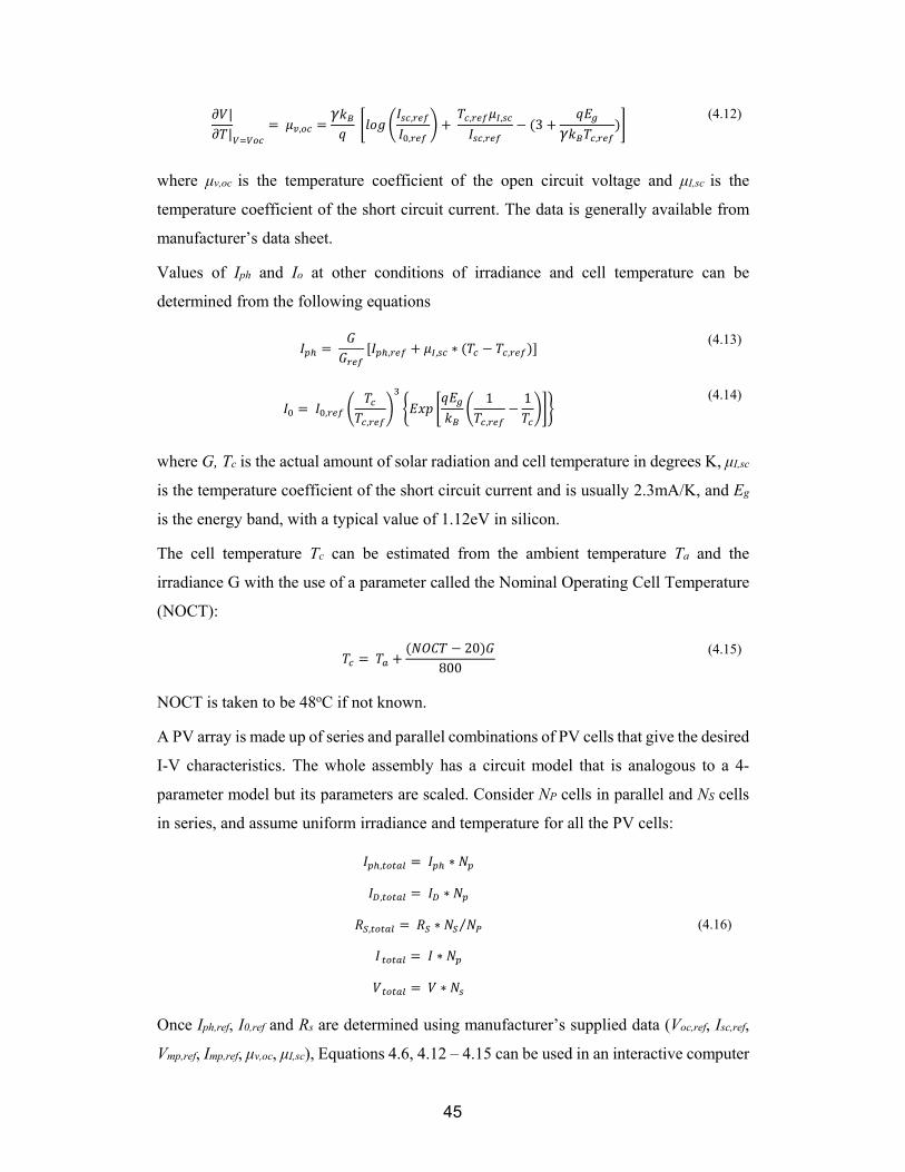
45

||

, ,

,

, ,

,3

,

(4.12)

where μv,oc is the temperature coefficient of the open circuit voltage and μI,sc is the

temperature coefficient of the short circuit current. The data is generally available from

manufacturer’s data sheet.

Values of Iph and Io at other conditions of irradiance and cell temperature can be

determined from the following equations

, , ∗ , (4.13)

,,

1

,

1

(4.14)

where G, Tc is the actual amount of solar radiation and cell temperature in degrees K, μI,sc

is the temperature coefficient of the short circuit current and is usually 2.3mA/K, and Eg

is the energy band, with a typical value of 1.12eV in silicon.

The cell temperature Tc can be estimated from the ambient temperature Ta and the

irradiance G with the use of a parameter called the Nominal Operating Cell Temperature

(NOCT):

20800

(4.15)

NOCT is taken to be 48oC if not known.

A PV array is made up of series and parallel combinations of PV cells that give the desired

I-V characteristics. The whole assembly has a circuit model that is analogous to a 4-

parameter model but its parameters are scaled. Consider NP cells in parallel and NS cells

in series, and assume uniform irradiance and temperature for all the PV cells:

, ∗

, ∗

, ∗ ⁄

∗

∗

(4.16)

Once Iph,ref, I0,ref and Rs are determined using manufacturer’s supplied data (Voc,ref, Isc,ref,

Vmp,ref, Imp,ref, μv,oc, μI,sc), Equations 4.6, 4.12 – 4.15 can be used in an interactive computer

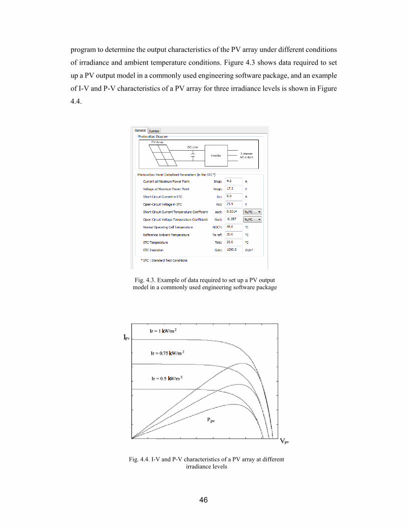
46

program to determine the output characteristics of the PV array under different conditions

of irradiance and ambient temperature conditions. Figure 4.3 shows data required to set

up a PV output model in a commonly used engineering software package, and an example

of I-V and P-V characteristics of a PV array for three irradiance levels is shown in Figure

4.4.

Fig. 4.3. Example of data required to set up a PV output model in a commonly used engineering software package

Fig. 4.4. I-V and P-V characteristics of a PV array at different irradiance levels

47

Inverter Modelling [69-72]

PV systems are connected to the grid via DC/AC inverters. Apart from performing

voltage conversion function from the DC output of the PV array to the AC voltage of the

grid and the associated grid interface functions such as power factor and anti-islanding

control, the inverters also incorporate Maximum Power Point Tracking (MPPT)

algorithm to ensure the maximum amount of power is extracted from the PV array. A

number of MPPT algorithms are in use such as open circuit voltage method, the

incremental conductance method, the ripple-based method, the parasitic capacitance

method and the perturbation and observation (P&O) technique. The MPPT algorithm

chosen will affect the conversion efficiency of the inverter and its response to transient

disturbances in the PV array output (such as those caused by passing clouds). For transient

studies the behaviour of the MPPT algorithm needs to be modelled.

Although the inverter topology structure can be complex, it has less impact on output

power calculation, which mainly depends on the relationship between its input and output

power, namely conversion efficiency. The conversion efficiency is made up of two main

components: MPPT efficiency which depends on the implementation of the MPPT

algorithm, and energy losses in the inverter. The latter is a function of input power to the

inverter:

, , (4.17)

where Ppv,n and Plosses are the inverter input power and losses normalised to the inverter

rating, with , ,

and

,.

The constants ko, k1 and k2 are specific to the inverter type being used and are generally

obtained via experimentation.

It is important to note that an undersized inverter will affect the inverter output, as the

inverter goes into power limiting mode when the input power (from the PV array output)

is higher than the rating of the inverter. An oversized inverter, on the other hand, suffers

from cost penalty and an inferior MPPT efficiency at lower PV array output due to the

difficulty in locating the maximum power point.

Solar Irradiance Modelling [69, 73, 74]

The photo-generated current (and hence output power) of the PV array is dependent on

the solar irradiance incident on the array surface – the plane-of-array (POA) solar

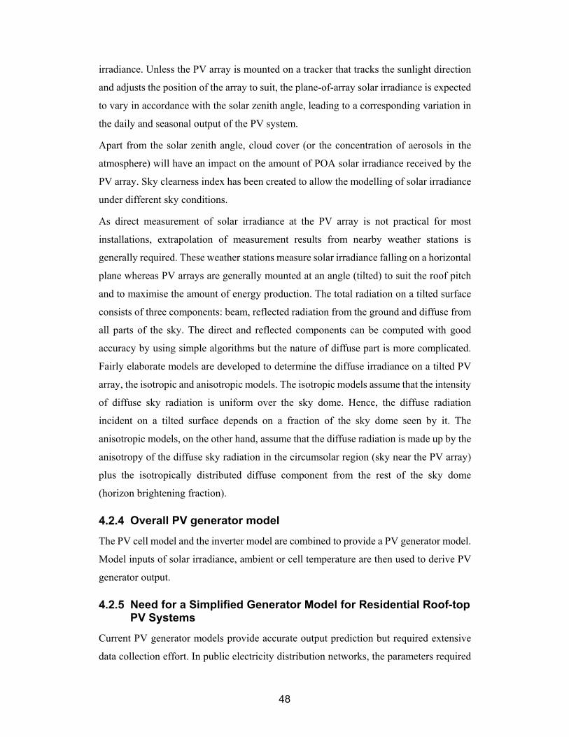
48

irradiance. Unless the PV array is mounted on a tracker that tracks the sunlight direction

and adjusts the position of the array to suit, the plane-of-array solar irradiance is expected

to vary in accordance with the solar zenith angle, leading to a corresponding variation in

the daily and seasonal output of the PV system.

Apart from the solar zenith angle, cloud cover (or the concentration of aerosols in the

atmosphere) will have an impact on the amount of POA solar irradiance received by the

PV array. Sky clearness index has been created to allow the modelling of solar irradiance

under different sky conditions.

As direct measurement of solar irradiance at the PV array is not practical for most

installations, extrapolation of measurement results from nearby weather stations is

generally required. These weather stations measure solar irradiance falling on a horizontal

plane whereas PV arrays are generally mounted at an angle (tilted) to suit the roof pitch

and to maximise the amount of energy production. The total radiation on a tilted surface

consists of three components: beam, reflected radiation from the ground and diffuse from

all parts of the sky. The direct and reflected components can be computed with good

accuracy by using simple algorithms but the nature of diffuse part is more complicated.

Fairly elaborate models are developed to determine the diffuse irradiance on a tilted PV

array, the isotropic and anisotropic models. The isotropic models assume that the intensity

of diffuse sky radiation is uniform over the sky dome. Hence, the diffuse radiation

incident on a tilted surface depends on a fraction of the sky dome seen by it. The

anisotropic models, on the other hand, assume that the diffuse radiation is made up by the

anisotropy of the diffuse sky radiation in the circumsolar region (sky near the PV array)

plus the isotropically distributed diffuse component from the rest of the sky dome

(horizon brightening fraction).

Overall PV generator model

The PV cell model and the inverter model are combined to provide a PV generator model.

Model inputs of solar irradiance, ambient or cell temperature are then used to derive PV

generator output.

Need for a Simplified Generator Model for Residential Roof-top PV Systems

Current PV generator models provide accurate output prediction but required extensive

data collection effort. In public electricity distribution networks, the parameters required

49

to determine these electrical models are not generally known as the PV panels are part of

private customer installations. A simplified, yet reasonably accurate PV generator model

is highly desirable.

Simplified Generator Model for Residential Roof-top PV Systems

Insight from Smart Meter Data

Residential PV installations in Australia are metered in two ways: gross metering where

separate channels are used to record load consumption and PV generation, and net

metering where a single channel (with separate export and import registers) is used to

record the aggregate load consumption and PV generation. An integrating time interval

of 30 minutes is commonly used. An example of a gross metering site with a 1kW PV

system is shown in Figure 4.5 where “GEN” is solar generation, “CON” is consumption

and “NET” is net consumption (derived using GEN and CON data). Negative values of

net consumption indicate net generation export from the customer premises.

A number of observations can be made from Figure 4.5:

The maximum output (averaged over 30 minutes) of the 1kW PV system is about

0.8kW on this day and this occurs between 12 to 1pm;

Where PV generation is higher than the consumption, the customer is exporting

energy back into the electricity network;

The customer has a peak usage at 4pm. As the PV is still generating at that time it is

able to contribute to peak reduction.

Fig. 4.5. Energy demand data of a customer with a 1kW PV system

‐1

‐0.5

0

0.5

1

1.5

2

2.5

3

00:00

01:00

02:00

03:00

04:00

05:00

06:00

07:00

08:00

09:00

10:00

11:00

12:00

13:00

14:00

15:00

16:00

17:00

18:00

19:00

20:00

21:00

22:00

23:00

Power (kW

)

1 Jan 2012

CONS

GEN

NET

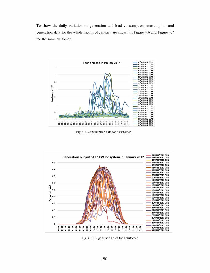
50

To show the daily variation of generation and load consumption, consumption and

generation data for the whole month of January are shown in Figure 4.6 and Figure 4.7

for the same customer.

Fig. 4.6. Consumption data for a customer

0

0.5

1

1.5

2

2.5

3

3.5

00:00

01:00

02:00

03:00

04:00

05:00

06:00

07:00

08:00

09:00

10:00

11:00

12:00

13:00

14:00

15:00

16:00

17:00

18:00

19:00

20:00

21:00

22:00

23:00

Load

 deman

d (kW

)

Load demand in January 2012 01/JAN/2012 CONS02/JAN/2012 CONS03/JAN/2012 CONS04/JAN/2012 CONS05/JAN/2012 CONS06/JAN/2012 CONS07/JAN/2012 CONS08/JAN/2012 CONS09/JAN/2012 CONS10/JAN/2012 CONS11/JAN/2012 CONS12/JAN/2012 CONS13/JAN/2012 CONS14/JAN/2012 CONS15/JAN/2012 CONS16/JAN/2012 CONS17/JAN/2012 CONS18/JAN/2012 CONS19/JAN/2012 CONS20/JAN/2012 CONS21/JAN/2012 CONS22/JAN/2012 CONS23/JAN/2012 CONS24/JAN/2012 CONS25/JAN/2012 CONS26/JAN/2012 CONS27/JAN/2012 CONS28/JAN/2012 CONS29/JAN/2012 CONS30/JAN/2012 CONS31/JAN/2012 CONS

Fig. 4.7. PV generation data for a customer

0

0.1

0.2

0.3

0.4

0.5

0.6

0.7

0.8

0.9

00:00

01:00

02:00

03:00

04:00

05:00

06:00

07:00

08:00

09:00

10:00

11:00

12:00

13:00

14:00

15:00

16:00

17:00

18:00

19:00

20:00

21:00

22:00

23:00

PV output (kW)

Generation output of a 1kW PV system in January 201201/JAN/2012 GEN02/JAN/2012 GEN03/JAN/2012 GEN04/JAN/2012 GEN05/JAN/2012 GEN06/JAN/2012 GEN07/JAN/2012 GEN08/JAN/2012 GEN09/JAN/2012 GEN10/JAN/2012 GEN11/JAN/2012 GEN12/JAN/2012 GEN13/JAN/2012 GEN14/JAN/2012 GEN15/JAN/2012 GEN16/JAN/2012 GEN17/JAN/2012 GEN18/JAN/2012 GEN19/JAN/2012 GEN20/JAN/2012 GEN21/JAN/2012 GEN22/JAN/2012 GEN23/JAN/2012 GEN24/JAN/2012 GEN25/JAN/2012 GEN26/JAN/2012 GEN27/JAN/2012 GEN28/JAN/2012 GEN29/JAN/2012 GEN30/JAN/2012 GEN31/JAN/2012 GEN

51

Energy consumption is generally recognized as a stochastic process and this is seen in

Figure 4.6 where the consumption data varies daily. Generation from the 1kW PV system

also exhibits significant variation from day to day as show in Figure 4.7. The peak output

of the PV system never reaches its nameplate rating of 1kW. This poses a challenge to

utility engineers to translate PV panel rating into capacity that can be used to support

network operation.

The variation in PV generation at the same site is due to a number of factors:

Solar irradiance falling on the PV panel surface exhibits seasonal variation due to

the changing angle of the sun’s ray.

Solar cell output exhibits a negative temperature coefficient with respect to cell

temperature. The process where sunlight is converted into electricity is therefore

less efficient on a hot day than a cold day.

Cloud cover affects the amount of solar irradiance that reaches the PV panel

surface. This is the primary factor that accounts for the randomness of solar

generation.

Figure 4.8 shows the maximum monthly generation output (kW) of a number of PV sites

over a one-year period. The outputs are averages over 30-minute intervals (not

instantaneous output). Seasonal variation of the maximum power output of the PV panels

Fig. 4.8. Maximum power output of a number of PV sites over the course of one year

0

0.5

1

1.5

2

2.5

3

3.5

4

Jan Feb Mar Apr May Jun Jul Aug Sep Oct Nov Dec

Maxim

um m

onthly PV Power Output (kW)

Maximum Monthly PV Generator Output for a Number of Gross Metering Sites

A

B

C

D

E

F

G

H

J

K

L

M

52

can be readily visualised. The lowest output occurs between June to August which

coincides with wet winter months in Victoria, Australia.

Derivation of a Simplified PV Generator Model

Cell temperature of a solar installation is not a parameter that can be easily measured. A

simplified empirical formula linking cell temperature to ambient temperature [64] is

given in Equation 4.15 and repeated here:

t t NOCT 20 ∗800

(4.18)

where Tc is the cell temperature, NOCT is the nominal operating cell temperature (taken

to be 48oC), and GPOA is the plane-of-array solar irradiance in Wm-2.

According to [75] the AC output of a PV system is given by

η (4.19)

t ∙1000

1 t 25 (4.20)

where PAC is the AC output of the PV inverter, PDC is the DC output of the PV array, η is

the dc/ac conversion efficiency (which includes the inverter MPPT and energy efficiency,

soiling and ageing of the PV array), PSTC is the PV panel dc rating specified at STC, and

CT is the temperature coefficient of PV cell (taken to be -0.5%/oC).

Combining Equations 4.18 - 4.20 gives

∙ η ∙1000

1.125 0.005 t 0.000175 (4.21)

Equation 4.21 can be used to model the AC output of a PV system using only ambient

temperature, solar irradiance and DC/AC conversion efficiency. There are a few

conditions for its use:

It is a quasi steady-state equation and cannot be used to determine the transient

response of a PV system to sudden changes in solar irradiance. The Maximum Power

Point Tracking (MPPT) algorithm incorporated in the inverter dominates the dynamic

behaviour of the PV system and has not been taken into account in the equation [71,

76]

DC/AC conversion efficiency is dependent on the amount of solar irradiance, soiling

and ageing of the PV panels, DC losses, inverter design and the amount of input power

53

relative to the inverter rating. The maximum AC output of a PV system normally

occurs at maximum solar irradiance where inverter efficiency is at its highest and a

nominal DC/AC conversion efficiency of 0.85 to 0.9 can be assumed [70]. For energy

yield calculation, [77] recommends an overall system derate factor (or efficiency) of

0.77.

Further simplification of Equation 4.21 is possible to improve its ease of use.

The plane-of-array solar radiation is made up of two components: a direct component

resulting from the sun’s direct beam, and a diffuse component resulting from scattering

of the sun's beam due to atmospheric constituents and reflection from surrounding objects

(the diffuse component is sometimes further split up into a diffuse component and a

reflected component). It can be expressed as below:

cos ϒ t1 cos α

2

(4.22)

where GDir is the direct irradiance measured in a plane normal to the sun, GDif is the diffuse

irradiance measured in the horizontal plane, α the inclination of the array from the

horizontal, and ϒ is the angle of incidence, between the direction of the sun’s ray and the

array normal, and is also known as the sun’s zenith distance.

Equation 4.22 can also be expressed using global irradiance GGlo, defined as the total solar

irradiance (both direct and diffuse) measured on the horizontal plane:

cos ϒ t (4.23)

Combining Equations 4.22 and 4.23 gives

tcos α 1

2

(4.24)

The inclination angle of the array (α) normally follows the pitch of the roof, with a typical

value of 22.5°. With GDif always smaller than GGlo (the two only become equal in a totally

overcast day where there is no direct ray from the sun), the second term in Equation 4.24

is less than 4% of the first term. We can therefore assume that GPOA is equal to GGlo.

Equation 4.21, which gives the output of a PV system, can now be further simplified using

GGlo:

η1000

1.125 0.005 t 0.000175 4.25

54

The maximum error introduced by this simplification is less than 1% when Equation 4.25

is used where the diffuse solar component is less than 20% of the global component, as

discussed in 4.4.1 below.

Applications of the Simplified PV Generator Model

Solar Irradiance Data at PV Locations

Unless local weather station has been installed, data for the solar irradiance falling on a

residential PV array is not readily available. To get around this limitation, tools developed

to determine the sizing of PV arrays and payback period generally use historic solar

statistics by establishing metrics such as Typical Meteorological Year (TMY) for a

particular region/country [77]. These solar irradiance data are useful for benchmarking

the annual energy yield of various PV systems. They are, however, not suitable for

predicting solar irradiance on shorter time horizons.

The Australian Bureau of Meteorology has a number of weather stations that measure

solar irradiance in time intervals of one second (averaged over a minute). The weather

station located at Tullamarine International Airport, in north-west of Melbourne, is in the

Fig. 4.9. Map of Jemena Electricity Networks

The area bounded by the blue contour is the electricity distribution network. The pink dots represent locations of PV systems. Location of the Tullamarine International Airport is shown by the call-out text box.

55

geographical centre of the Jemena Electricity Networks where these PV systems are

installed (Figure 4.9). The solar irradiance recorded at this weather station [78] is used as

the ‘proxy’ for the solar irradiance received by PV arrays located in any part of the

electricity distribution network.

To test the validity of this assumption, a linear correlation study is performed between

the global solar irradiance daily dataset and the generation daily dataset of a 1kW PV

system over a one-year period (2012). As the generation dataset is only available in 30-

minute aggregate values, the 1-second solar irradiance data (Wm-2) are firstly aggregated

to form 30-minue solar irradiance energy (Jm-2).

The MATLAB function corrcoef is then run for the data matrix (where each column

represents a separate quantity). A positive linear relationship between the data columns

will return a matrix of correlation coefficients with values close to 1. The correlation

coefficients are plotted in Figure 4.10 and also summarized in Table 4.1.

Table 4.1 Summary of correlation coefficients

Value of correlation coefficient Days Percentage of days in 2012

>=0.95 183 51.50%

>=0.90 257 72.40%

>=0.85 306 86.20%

Fig. 4.10. Daily correlation coefficients for the 1kW PV customer site

‐0.4

‐0.2

0

0.2

0.4

0.6

0.8

1

1.2

1st 3rd 5th 7th 9th 11th 13th 15th 17th19th 21st 23rd 25th 27th 29th 31stCorrelation coefficien

ts

Days of Month

Correlation coefficients for PV site A

Jan‐12

Feb‐12

Mar‐12

Apr‐12

May‐12

Jun‐12

Jul‐12

Aug‐12

Sep‐12

Oct‐12

Nov‐12

Dec‐12

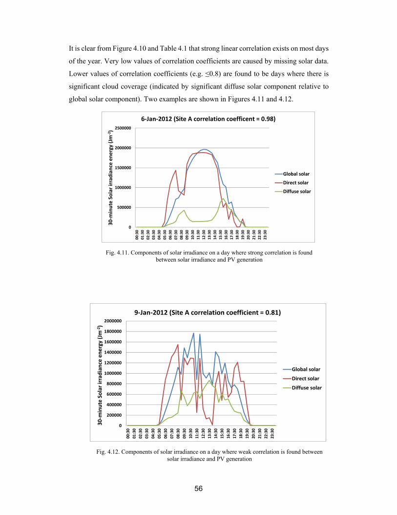
56

It is clear from Figure 4.10 and Table 4.1 that strong linear correlation exists on most days

of the year. Very low values of correlation coefficients are caused by missing solar data.

Lower values of correlation coefficients (e.g. ≤0.8) are found to be days where there is

significant cloud coverage (indicated by significant diffuse solar component relative to

global solar component). Two examples are shown in Figures 4.11 and 4.12.

Fig. 4.11. Components of solar irradiance on a day where strong correlation is found between solar irradiance and PV generation

0

500000

1000000

1500000

2000000

2500000

00:30

01:30

02:30

03:30

04:30

05:30

06:30

07:30

08:30

09:30

10:30

11:30

12:30

13:30

14:30

15:30

16:30

17:30

18:30

19:30

20:30

21:30

22:30

23:30

30‐m

inute Solar irradiance energy (Jm

‐2)

6‐Jan‐2012 (Site A correlation coefficent = 0.98)

Global solar

Direct solar

Diffuse solar

Fig. 4.12. Components of solar irradiance on a day where weak correlation is found between solar irradiance and PV generation

0

200000

400000

600000

800000

1000000

1200000

1400000

1600000

1800000

2000000

00:30

01:30

02:30

03:30

04:30

05:30

06:30

07:30

08:30

09:30

10:30

11:30

12:30

13:30

14:30

15:30

16:30

17:30

18:30

19:30

20:30

21:30

22:30

23:30

30‐m

inute Solar irradiance energy (Jm

‐2)

9‐Jan‐2012 (Site A correlation coefficient = 0.81)

Global solar

Direct solar

Diffuse solar

57

Solar irradiance on a clear-sky day is dominated by the direct solar irradiance component

and one would expect that this direct component will be experienced by PV panels

installed in relative close proximity to the weather station. On a cloudy day, however,

solar irradiance has a significant diffuse component. This diffuse component is caused by

scattering of the sun’s ray by cloud and surrounding objects, including reflection from the

ground. The diffuse component can show significant variation depending on the local site

condition and the measurements taken at Tullamarine weather station may not be

representative.

Similar observation is obtained from analysis of other PV sites. It is therefore concluded

that the aggregate (30-minute) solar irradiance data at the Tullamarine weather station is

a reasonable ‘proxy’ to model the solar irradiance received by a local PV system on a

clear sky day, when the diffuse solar irradiance contributes less than 20% to the global

solar irradiance.

As shown later in Section 4.4.3, the proposed PV output model has also been used in

predicting the one-minute output profile of PV system in a power quality investigation,

using one-minute solar and 30-minute ambient temperature data from the Tullamarine

weather station. It looks promising that the proposed approach to the solar irradiance data

will be accurate enough to simulate the steady-state output of a PV system down to 1-

minute time horizon.

Solar forecasting is under active research currently. It is possible that accurate solar

forecast data will become available soon [79] which can then be used as ‘proxy’ to

forecast the output of PV systems in day-ahead planning studies.

Modelled and Actual Output of a PV System

Equation 4.25 provides the quasi steady-state output of a PV system at any time t,

provided the global solar irradiance and ambient temperature at that instance in time are

known. While instantaneous value of the PV system output is useful for power quality

impact assessment, utility planning engineers are more interested in 'average' PV output

over a time interval, typically 30-minute, as this aligns with the thermal inertia of

equipment commonly found in electrical power networks. This can be achieved by

summating the calculated PV output, at every second, over a 30-minute interval, then

dividing the summation by the time interval (1800 seconds), as per Equation 4.26:

58

11800

∙ η0.0011800

1.125 0.005 t ∙

0.000175

4.26

For the time varying quantities on the right-hand side of Equation 4.26, global solar

irradiance GGlo is available from the Bureau of Meteorology weather station while

ambient temperature measurements are only available as 30-minute snapshots which are

considered acceptable as ambient temperature does not exhibit rapid variation. Finally for

maximum output determination, the efficiency η is taken as 0.9.

The 30-minute generation output of the 1kW PV site is determined using Equation 4.26,

and compared with the measured generation output by smart meter. The results for 2 days

in January 2012 are shown in Figures 4.13 and 4.14. On 2 January the sky was overcast

(shown by the high diffuse to global solar irradiance ratio) whereas the sky was relatively

clear on 6 January. It can be seen that Equation 4.26 gives an accurate estimate of 30-

minute generation output when cloud cover is minimal, reinforcing the observation made

in Section 4.4.1 above.

Fig. 4.13. Actual and estimated output of a 1kW PV system on a relatively cloudy day

59

It should be noted that the error of Equation 4.26 is larger at low PV output. This is due

to the fact that the PV inverter is generally less efficient at low power (corresponding to

low solar irradiance level early in the morning or late in the afternoon) [70]. This is not

considered a limitation when Equation 4.26 is used for the purpose of determining the

maximum output of a PV system.

While the accuracy of the approach cannot be determined analytically, the error of peak

power prediction in the sample of the PV systems modelled varies from -0.2% to 7.8%.

It can be concluded that the output of a PV system can be estimated reasonably accurately

by the proposed method, provided the solar irradiance data used in the calculation (and

measured at a nearby weather station) has only a small diffuse component, and that the

solar system is operating at high output level relative to its rating.

Power Quality Investigations

Jemena Electricity Networks, who contributes data to this research project, has been

experiencing increasing level of overvoltage complaints from its customers who have

installed PV systems. Complaints are generally related to the loss of revenue caused by

the inability to export surplus PV power when the PV inverters trip on overvoltage

occurrences. On receiving the complaint, the company initiates power quality

investigation by installing portable power quality meters at the supply substation and the

customer supply point, recording voltages, currents and other related quantities (such as

power factor and harmonics) over a one-week period. The results are then analysed and

remedial action taken if the supply voltages are found to be outside the regulatory limits.

Fig. 4.14. Actual and estimated output of a 1kW PV system on a relatively clear sky day

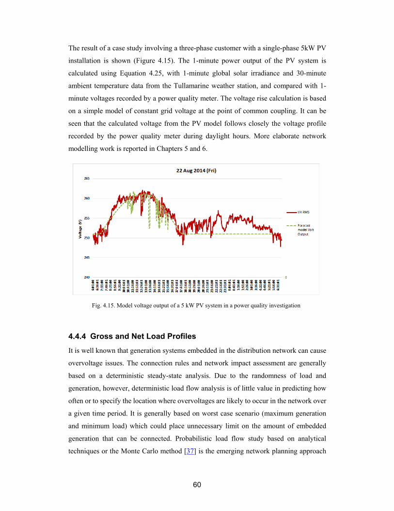
60

The result of a case study involving a three-phase customer with a single-phase 5kW PV

installation is shown (Figure 4.15). The 1-minute power output of the PV system is

calculated using Equation 4.25, with 1-minute global solar irradiance and 30-minute

ambient temperature data from the Tullamarine weather station, and compared with 1-

minute voltages recorded by a power quality meter. The voltage rise calculation is based

on a simple model of constant grid voltage at the point of common coupling. It can be

seen that the calculated voltage from the PV model follows closely the voltage profile

recorded by the power quality meter during daylight hours. More elaborate network

modelling work is reported in Chapters 5 and 6.

Gross and Net Load Profiles

It is well known that generation systems embedded in the distribution network can cause

overvoltage issues. The connection rules and network impact assessment are generally

based on a deterministic steady-state analysis. Due to the randomness of load and

generation, however, deterministic load flow analysis is of little value in predicting how

often or to specify the location where overvoltages are likely to occur in the network over

a given time period. It is generally based on worst case scenario (maximum generation

and minimum load) which could place unnecessary limit on the amount of embedded

generation that can be connected. Probabilistic load flow study based on analytical

techniques or the Monte Carlo method [37] is the emerging network planning approach

Fig. 4.15. Model voltage output of a 5 kW PV system in a power quality investigation

61

that takes into account the stochastic nature of intermittent renewable generation (such as

PV) and load.

An inherent requirement for any probabilistic load flow technique is the determination of

Probability Density Functions (PDFs) of the loads based on historic load profiles. With

the increasing penetration of PV generation in the electricity distribution network, the

historic load profiles measured at various network assets (such as distribution

transformers, distribution lines) are net profiles combining the effect of electricity usage

and PV generation. As PV generation and load consumptions are affected by different

external factors, their PDFs do not follow the same probability distribution curve. To use

probabilistic load flow technique, the net load profiles should be disaggregated into load

and generation profiles before PDFs are determined. This can be achieved by using the

PV model established in Section 4.4.2.

Let X(t) be a random variable representing 30-minute energy data measured by the smart

meter, Y(t) be the corresponding random variable of 30-minute solar generation, and Z(t)

the random variable of energy consumption within the premise. The three random

variables have the following relationship at time instant t:

4.27

As X(t) is known and Y(t) can be estimated by Equation 4.26, Z(t) can be determined.

To illustrate the concept, load and generation data from the gross metering PV site are

aggregated together to form net load profile. Generation output is then calculated using

Equation 4.26, after which the load profile is derived using Equation 4.27, and compared

with the metered load data. The results are shown in Figure 4.16. The estimation error at

low PV output can be improved by fitting a curve for the PV efficiency η at different

output power levels, rather than the use of a single (high) value.

Many PV sites in Australia have net metering applied where a single meter (with separate

export and import registers/channels) is used to record the aggregate energy flow into or

out of the point of connection. In other words, the energy recorded by the meter represents

the net consumption/generation of the site. The above approach can be used to

disaggregate the net metering data into load and generation data.

62

Summary

One of the major challenges faced by the electrical supply industry in accommodating

customer PV installations today is delivering secure, reliable and high quality power

while managing voltage rise, fluctuations and intermittency of the energy source. Meeting

the challenge requires knowledge about real-life output of the installed PV systems.

Significant work has been carried out by the international research community to develop

mathematical models of PV arrays for applications including energy forecasting,

economic payback assessment, electricity network impact assessment and transient

stability. Simplification of these models, however, is required for practical applications

in electricity distribution networks, particularly for small roof-top PV installations. This

chapter provides utility engineers a tool to efficiently determine the in-situ output of roof-

top PV systems installed on customer premises, without the need for extensive data

collection. The methodology is based on DC rating of the PV system, ambient

temperature and solar irradiance data. To overcome the challenge posed by the lack of

local measurements of solar irradiance data, covariance analysis has confirmed that data

captured in a nearby weather station can be used provided the sky is relatively clear.

While this constraint may seem to be limiting, the methodology is applicable to electricity

network studies which have the focus on extremes (such as maximum solar irradiance

and clear sky) rather than averages.

Fig. 4.16. Estimated and measured load profile for the 1kW PV site

63

As penetration of PV system increases in electricity distribution network, it would

become necessary to disaggregate load measurements captured by monitoring systems

(such as smart meters and SCADA) into solar generation and load consumption. This will

allow the appropriate drivers to be incorporated into the analysis of historic data and

future forecast. In this regard, it is important to point out that load demand in Australia is

generally driven by air conditioning use during hot summer days, many of which are

coincident with dense cloud cover. As solar output is reduced at high ambient temperature

and cloud coverage, it is important to extract generation output from load data to allow

separate forecasting methodology to be applied.

The use of the PV generator model is further explored in Chapters 5 and 6.

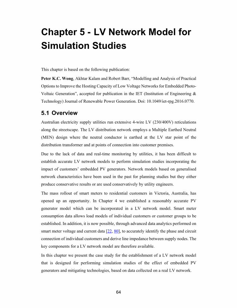
64

Chapter 5 - LV Network Model for

Simulation Studies

This chapter is based on the following publication:

Peter K.C. Wong, Akhtar Kalam and Robert Barr, “Modelling and Analysis of Practical

Options to Improve the Hosting Capacity of Low Voltage Networks for Embedded Photo-

Voltaic Generation”, accepted for publication in the IET (Institution of Engineering &

Technology) Journal of Renewable Power Generation. Doi: 10.1049/iet-rpg.2016.0770.

Overview

Australian electricity supply utilities run extensive 4-wire LV (230/400V) reticulations

along the streetscape. The LV distribution network employs a Multiple Earthed Neutral

(MEN) design where the neutral conductor is earthed at the LV star point of the

distribution transformer and at points of connection into customer premises.

Due to the lack of data and real-time monitoring by utilities, it has been difficult to

establish accurate LV network models to perform simulation studies incorporating the

impact of customers’ embedded PV generators. Network models based on generalised

network characteristics have been used in the past for planning studies but they either

produce conservative results or are used conservatively by utility engineers.

The mass rollout of smart meters to residential customers in Victoria, Australia, has

opened up an opportunity. In Chapter 4 we established a reasonably accurate PV

generator model which can be incorporated in a LV network model. Smart meter

consumption data allows load models of individual customers or customer groups to be

established. In addition, it is now possible, through advanced data analytics performed on

smart meter voltage and current data [22, 80], to accurately identify the phase and circuit

connection of individual customers and derive line impedance between supply nodes. The

key components for a LV network model are therefore available.

In this chapter we present the case study for the establishment of a LV network model

that is designed for performing simulation studies of the effect of embedded PV

generators and mitigating technologies, based on data collected on a real LV network.

65

Network Asset Data

The network model is set up from the source MV zone substation. This approach is taken

so that the voltage regulating devices on the MV network are included in the modelling

and simulation. The distribution circuit used in the case study is a 22kV/433V distribution

substation (Cypress-Stillia) supplied by 22kV feeder (SHM14) from SHM 66/22kV Zone

Substation. The circuit forms part of the electricity distribution network operated by

Jemena, an electricity distribution company in the state of Victoria, Australia.

The MV supply network and the LV distribution circuit have the characteristics shown in

Table 5.1. Figures 5.1 and 5.2 provide geographic view of the LV distribution circuits

and the details of LV distribution circuit #4.

Table 5.1 Network Characteristics (provided by Jemena Electricity Networks)

Circuit Element Characteristics

Supply source (SHM 66kV side)

3-phase fault level = 7.1kA, 1-phase fault level = 4.0kA, voltage regulated at 67kV.

SHM 66/22kV transformers 40MVA, 66/22kV, delta/star, tap winding = 66kV, tapping range = 0.95 to 1.05, tap number = 16, impedance = 10% on 40MVA.

22kV feeder SHM14 Six overhead circuit segments, with a distribution substation at the end of each circuit segment. The overhead lines are 3-wire 19/3.25AAC. Note the MV feeder characteristics has been simplified to reduce the complexity of modelling work.

Cypress-Stillia distribution substation

Connected to the end of the fifth 22kV circuit segment. Comprises of a transformer: 300kVA, 22/0.433kV, delta/star, tap winding = 22kV, tapping range = 0.925 to 1.025, tap number = 4, impedance = 4% on 300kVA.There are 38 customers supplied from this substation arranged in three LV distribution circuits.

LV Distribution Circuit #4 (coloured brown in Figure 1) ex Cypress-Stillia distribution substation

Underground cables supplying eight customers. The cable forming the LV backbone is 185mm2 Al 4/C while the branch cable is 16mm2 Cu 4/C.

Customer details on LV Distribution Circuit #4

Customer Supply Max Load PV

Cus 1 3-phase 5kVA

Cus 2 B-phase 5kVA

Cus 3 3-phase 15kVA

Cus 4 3-phase 7.8kVA

Cus 5 3-phase 7kVA 4kW

Cus 6 W-phase 5kVA

Cus 7 3-phase 9kVA 5kW

Cus 8 3-phase 9KVA

66

Derivation of Line Impedances

The Need to Model Neutral Conductor and Earth

The 22kV feeder backbone of SHM14 comprises of 3-phase, 3-wire overhead conductors,

single-point earthed on the 22kV neutral of the 66/22kV transformer. We have simplified

the backbone structure to six overhead line segments and lumped loads at each segment

node. The three LV distribution circuits of Cypress-Stillia supply 38 customers via 3-

phase, 4-wire underground cables (backbone & 3-phase customers) and 1-phase, 2-wire

underground cables for 1-phase customers. A Multiple Earthed Neutral (MEN) system is

implemented where the neutral conductors are earthed at customer points of connection

(POC) as well as at the LV star point of the supply distribution transformer. The neutral

to earth impedance is taken to be 10 ohms at the supply distribution substation and 100

ohms at the customer POC based on design standard and empirical measurements. For

LV network modelling it is more accurate to model both the neutral conductor and the

earth connections as the loads are inherently unbalanced (due to 1-phase customer

connections) so currents will flow in both the neutral conductor and earth, leading to

Fig. 5.1. LV Distribution Circuits from Cypress Stillia Distribution Substation

Fig. 5.2. Details of LV Distribution Circuit #4

67

voltages appearing on the neutral conductor. It is important to note that most load flow

software packages return phase-to-ground voltage results whereas the voltages received

by customer equipment are the voltages between phases and neutral. Care should be taken

to interpret load flow results when ground and neutral are not at the same potential [81].

In addition, neutral-point shifting will cause voltage increase to occur in one phase while

voltage decrease in the other two phases. Ignoring the neutral conductor in modelling will

therefore lead to erroneous results [82].

Calculating LV Line Impedances Considering Neutral Conductor and Earth

For line impedances, the series impedances published by the suppliers (positive, negative

and zero sequence) for the overhead lines and cables normally assume physical symmetry

between the three phase and neutral conductors. This is generally not a true representation

of the MV distribution network as 2-wire 2-phase tee-offs are common especially in rural

areas, and there is no regular transposition of the three phase conductors. Where high

accuracy is required MV networks should therefore be modelled as a 3-phase unbalanced

system. The LV distribution system consists of single-phase, two-phase, and un-

transposed three-phase lines serving loads that are mostly connected between phase and

neutral. For LV line impedance determination, it is necessary to retain the self and mutual

impedance terms of the conductors and take into account the ground return path for the

unbalanced currents. A commonly used approach to calculate line impedances are the

Carson’s equations. Carson assumes the earth is an infinite, uniform solid with a flat

uniform upper surface and a constant resistivity. The equations of self and mutual

impedances made use of conductor images; that is, every conductor at a given distance

above ground has an image conductor the same distance below ground. The concept is

illustrated in Figure 5.3.

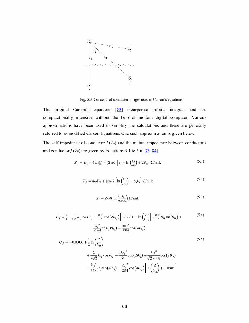
68

The original Carson’s equations [83] incorporate infinite integrals and are

computationally intensive without the help of modern digital computer. Various

approximations have been used to simplify the calculations and these are generally

referred to as modified Carson Equations. One such approximation is given below.

The self impedance of conductor i (Zii) and the mutual impedance between conductor i

and conductor j (Zij) are given by Equations 5.1 to 5.6 [33, 84].

4ωP j2ωG ln 2 Ω/mile (5.1)

4ωP j2ωG ln 2 Ω/mile (5.2)

2ωG ln Ω/mile (5.3)

√cos cos 2 0.6728 ln + sin

√ ∗

cos 3 cos 4

(5.4)

0.038612ln

2

1

3√2cos 64

cos 2√2 ∗ 45

cos 3

384sin 4

384cos 4 ln

21.0985

(5.5)

Fig. 5.3. Concepts of conductor images used in Carson’s equations

69

8.565 x 10 (5.6)

where i = j = 1, 2 …. ncond

ncond = number of conductors

Zii = self impedance of conductor i in Ω/mile

Zij = mutual impedance between conductors i and j in Ω/mile

ri = resistance of conductor i in Ω/mile

G = 0.1609347 * 10-3 Ω/mile

ω = 2πf = system angular frequency in radians per second

Ri = radius of conductor i in feet

GMRi = Geometric Mean Radius of conductor i in feet

f = system frequency in Hertz

ρ = resistivity of earth in Ω-metres

Dij = distance between conductors i and j in feet (see Figure 5.2)

Sij = distance between conductor i and image j in feet (see Figure 5.2)

θij = angle between a pair of lines drawn from conductor i to its own image and to

the image of conductor j (see Figure 5.2)

These equations can be further modified to reduce the computational effort without

sacrificing too much of accuracy [33] by reducing the number of terms in Equations 5.4

and 5.5:

8 (5.7)

0.038612ln

2

(5.8)

These modified Carson’s equations, as they come to be called, are used extensively.

Applying the modified Carson’s equations to a 4-wire LV line (a, b, c, n) will result in a

primitive impedance matrix of [4 x 4]:

70

(5.9)

(5.10)

Kron reduction can be used to reduce Zline to a 3x3 phase impedance matrix however this

is not recommended as we are interested to know the voltage on the neutral conductor.

Work examples to derive line and cable parameters from manufacturer data and physical

construction can be found in [33, 84].

The modelling software, as detailed in Section 5.6, uses the modified Carson’s equations

to derive line and cable impedance parameters and is well suited for the application

described herein.

Derivation of Loads and Generation

Load Modelling

Customer load models are set up based on SCADA and smart meter measurements over

a summer week from 15 to 21 February 2015 when the daily ambient temperature varied

from 14.5oC to 35oC. This week of data is chosen in the case study because it represents

a wide range of load consumption which the supply network needs to accommodate, and

impact of PV generation is generally at its highest during summer months. The loads are

modelled as PQ loads and are specified in base load format (kVA, constant power factor).

The base loads are modified by loadshapes to gives time series variations of load over the

course of the week. The methodology for the derivation of base loads and loadshapes is

shown in Table 5.2.

Care has been exercised to ensure the load models closely resemble actual customer loads.

Figure 5.4 shows the loadshapes used in the weekly simulation, while Figure 5.5 shows

the daily loadshapes in more details for 15 February 2015.

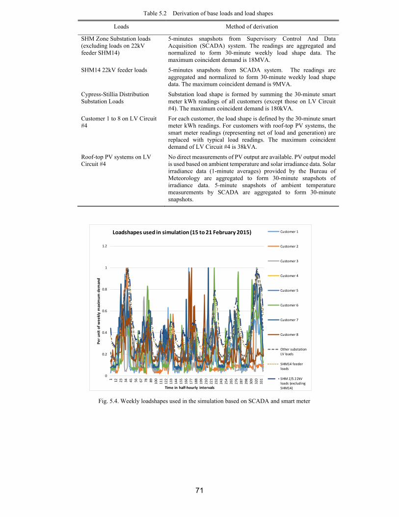
71

Table 5.2 Derivation of base loads and load shapes

Loads Method of derivation

SHM Zone Substation loads (excluding loads on 22kV feeder SHM14)

5-minutes snapshots from Supervisory Control And Data Acquisition (SCADA) system. The readings are aggregated and normalized to form 30-minute weekly load shape data. The maximum coincident demand is 18MVA.

SHM14 22kV feeder loads 5-minutes snapshots from SCADA system. The readings are aggregated and normalized to form 30-minute weekly load shape data. The maximum coincident demand is 9MVA.

Cypress-Stillia Distribution Substation Loads

Substation load shape is formed by summing the 30-minute smart meter kWh readings of all customers (except those on LV Circuit #4). The maximum coincident demand is 180kVA.

Customer 1 to 8 on LV Circuit #4

For each customer, the load shape is defined by the 30-minute smart meter kWh readings. For customers with roof-top PV systems, the smart meter readings (representing net of load and generation) are replaced with typical load readings. The maximum coincident demand of LV Circuit #4 is 38kVA.

Roof-top PV systems on LV Circuit #4

No direct measurements of PV output are available. PV output model is used based on ambient temperature and solar irradiance data. Solar irradiance data (1-minute averages) provided by the Bureau of Meteorology are aggregated to form 30-minute snapshots of irradiance data. 5-minute snapshots of ambient temperature measurements by SCADA are aggregated to form 30-minute snapshots.

Fig. 5.4. Weekly loadshapes used in the simulation based on SCADA and smart meter

0

0.2

0.4

0.6

0.8

1

1.2

1

12

23

34

45

56

67

78

89

100

111

122

133

144

155

166

177

188

199

210

221

232

243

254

265

276

287

298

309

320

331

Per unit of weekly maxim

um deman

d 

Time in half‐hourly  intervals

Loadshapes used in simulation (15 to 21 February 2015) Customer 1

Customer 2

Customer 3

Customer 4

Customer 5

Customer 6

Customer 7

Customer 8

Other substationLV loads

SHM14 feederloads

SHM Z/S 22kVloads (excludingSHM14)

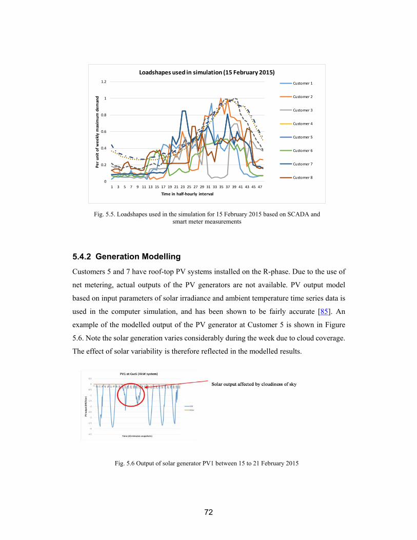
72

Generation Modelling

Customers 5 and 7 have roof-top PV systems installed on the R-phase. Due to the use of

net metering, actual outputs of the PV generators are not available. PV output model

based on input parameters of solar irradiance and ambient temperature time series data is

used in the computer simulation, and has been shown to be fairly accurate [85]. An

example of the modelled output of the PV generator at Customer 5 is shown in Figure

5.6. Note the solar generation varies considerably during the week due to cloud coverage.

The effect of solar variability is therefore reflected in the modelled results.

Fig. 5.5. Loadshapes used in the simulation for 15 February 2015 based on SCADA and smart meter measurements

0

0.2

0.4

0.6

0.8

1

1.2

1 3 5 7 9 11 13 15 17 19 21 23 25 27 29 31 33 35 37 39 41 43 45 47

Per unit of weekly maxim

um deman

d 

Time in half‐hourly  interval

Loadshapes used in simulation (15 February 2015)

Customer 1

Customer 2

Customer 3

Customer 4

Customer 5

Customer 6

Customer 7

Customer 8

Fig. 5.6 Output of solar generator PV1 between 15 to 21 February 2015

73

Modelling of Voltage Control Devices

As a distribution network, JEN takes supply from the transmission substations primarily

at 66kV. The voltages at the transmission substations are nominated by the distribution

network service provider (in this case, JEN) and maintained by the transmission network

service provider. Voltage regulation on the distribution network is achieved via a number

of voltage control devices. Table 5.3 summarises the voltage control devices included in

the network model. Some of these voltage control devices are currently utilized by JEN

while others are being considered for future.

Table 5.3 Voltage Control Devices

Device Function

On-load tap changer (OLTC) on 66/22kV transformer

Change the voltage on the 22kV side of the transformer by changing the ratio of the 66kV winding. The voltage control settings are implemented in the voltage regulating relay (VRR).

Substation capacitor banks

Adjust 22kV bus voltage by compensating for the reactive component of the customer loads. Arranged in two steps of 4MVar (3-ph) each.

Line capacitor banks Adjust 22kV line voltage by switching pole-mounted capacitors to compensate for the reactive component of the customer loads flowing through the 22kV distribution line. Single step of 900kVar (3-ph) each.

22/0.433kV distribution transformer

The transformer is fitted with off-load tap changer on the 22kV side. It is generally set on tap 1 (22.55/0.433kV) at time of commissioning.

22/0.415kV smart grid distribution transformer (future)

The transformer is fitted with on-load tap changer on the 22kV side. The transformer specification used in the simulation consists of off-load tap +/-5% with 5 taps, and on-load tap +/-5% with 5 taps.

Smart PV inverter (future)

Smart inverters fitted to PV generators to reduce their impact on network voltage while generating and/or to assist network voltage by acting as a DSTATCOM.

Storage battery (future) Storage battery can assist with voltage changes caused by PV generation, by charging from excess PV generation during the day and discharging during the evening peak load period.

Modelling Software

The network model is set up in the Open Distribution System SimulatorTM (OpenDSS),

an open-source electrical system simulation tool for utility distribution systems, made

available by the Electric Power Research Institute, Inc. (EPRI) [86]. OpenDSS includes

comprehensive library of power delivery elements such as generators, transformers, lines,

PV generators, storage batteries as well as control elements such as regulator control and

capacitor bank control. Scripting is performed using text files. The flexibility and

versatility of OpenDSS is further expanded by the use of an in-process Component Object

Model (COM) interface which allows an external program to drive the various OpenDSS

74

functions, provides external analytical capabilities as well as graphics for displaying

results. In this research, MATLAB® is used to drive OpenDSS through the COM

interface.

The network model is set up in OpenDSS based on the network characteristics of Table

5.1 and load characteristics of Table 5.2. For line impedances, OpenDSS uses two

different methods to represent line impedances: LineCode objects requires input of

impedance characteristics while LineGeometry objects uses wire data and positions of

the conductors to compute the impedance matrix using modified Carson’s equations. A

simple example of an OpenDSS program to compute the impedance matrix for a typical

4-wire LV line using 19/3.25AAC conductors is shown in Figure 5.7. The program output

is shown in Figure 5.8 and the impedance matrix is reproduced in Table 5.4 for clarity.

Fig. 5.7. Example OpenSS codes for converting a 4-wre LV line construction into impedance matrix

Fig. 5.8. Output of OpenDSS codes for a 4-wire LV line

75

Table 5.4 Impedance Matrix for 4-wire 19/3.25AAC LV Overhead Line

Phase a Phase b Phase c Neutral

0.241234 + j0.75306

0.0486496 +j0.418661

0.0486496 + j0.394817

0.0486497 +j0.467242 Phase a

0.0486496 +j0.418661 0.241234 +j0.75306

0.0486497 +j0.467242

0.0486497 +j0.457556 Phase b

0.0486496 + j0.394817

0.0486497 +j0.467242

0.241234 + j0.75306

0.0486496 + j0.418661 Phase c

0.0486497 +j0.467242

0.0486497 +j0.457556

0.0486496 + j0.418661 0.241234 +j0.75306 Neutral

The circuit in OpenDSS allows explicit modelling of the ground connections and this

feature is used in modelling the MEN LV network.

Figure 5.9 shows the single-line representation of the network model that has been set up

in OpenDSS. Monitors have been allocated to various line terminals and buses to record

power parameters during simulation studies.

76

Network Scenarios Modelled

The set of network scenarios (1 to 8) considers the effectiveness of various MV voltage

control schemes in regulating the voltage on the 433V side of the Cypress-Stillia

distribution transformer (Table 5.5). The voltage control schemes as outlined in Table 5.3

are considered except smart grid distribution transformer, smart PV inverter and storage

battery. These MV voltage control schemes are commonly deployed by distribution

Fig. 5.9. Single-line presentation of network model

77

utilities and their fine tuning generally represents a low-cost approach to increase the

hosting capacity of PV generators by the distribution networks.

The loads served by SHM 66/22kV transformer are primarily residential in nature and so

are the loads on SHM14 22kV feeder, as revealed by the SCADA readings (Figure 5.10).

It is, however, not unusual for a 66/22kV substation to serve a mixture of residential,

commercial and industrial customers. The network scenarios 7 and 8 consider assigning

different load types (Figure 5.11) to the remaining loads served by the 66/22kV substation

while keeping the SHM14 22kV feeder load as residential. These scenarios explore the

balancing act of meeting the needs of different classes of customers.

Fig. 5.10. SCADA readings of loads on SHM Zone Substation and SHM14 feeder

0.00

5.00

10.00

15.00

20.00

25.00

30.00

0.00

50.00

100.00

150.00

200.00

250.00

300.00

1

15

29

43

57

71

85

99

113

127

141

155

169

183

197

211

225

239

253

267

281

295

309

323

Amps

MVA

Half‐hourly

Loading between 15 to 21 February 2015 

SHM14 Feeder Current (A) SHM Zone Sub (MVA)

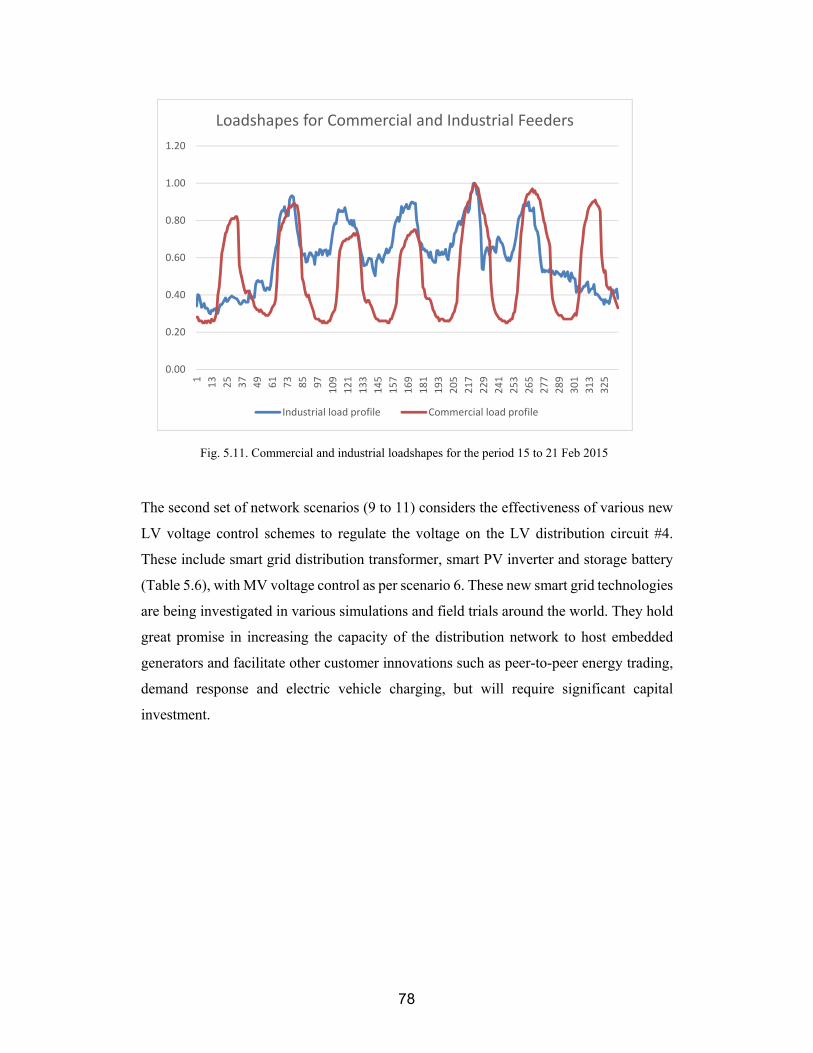
78

The second set of network scenarios (9 to 11) considers the effectiveness of various new

LV voltage control schemes to regulate the voltage on the LV distribution circuit #4.

These include smart grid distribution transformer, smart PV inverter and storage battery

(Table 5.6), with MV voltage control as per scenario 6. These new smart grid technologies

are being investigated in various simulations and field trials around the world. They hold

great promise in increasing the capacity of the distribution network to host embedded

generators and facilitate other customer innovations such as peer-to-peer energy trading,

demand response and electric vehicle charging, but will require significant capital

investment.

Fig. 5.11. Commercial and industrial loadshapes for the period 15 to 21 Feb 2015

0.00

0.20

0.40

0.60

0.80

1.00

1.20

1

13

25

37

49

61

73

85

97

109

121

133

145

157

169

181

193

205

217

229

241

253

265

277

289

301

313

325

Loadshapes for Commercial and Industrial Feeders

Industrial load profile Commercial load profile

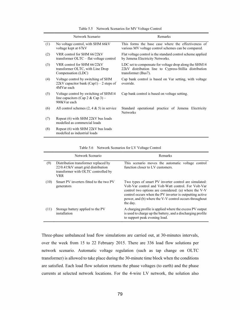
79

Table 5.5 Network Scenarios for MV Voltage Control

Network Scenario Remarks

(1) No voltage control, with SHM 66kV voltage kept at 67kV

This forms the base case where the effectiveness of various MV voltage control schemes can be compared.

(2) VRR control for SHM 66/22kV transformer OLTC – flat voltage control

Flat voltage control is the standard control scheme applied by Jemena Electricity Networks.

(3) VRR control for SHM 66/22kV transformer OLTC, with Line Drop Compensation (LDC)

LDC set to compensate for voltage drop along the SHM14 22kV distribution line to Cypress-Stillia distribution transformer (Bus7).

(4) Voltage control by switching of SHM 22kV capacitor bank (Cap1) – 2 steps of 4MVar each

Cap bank control is based on Var setting, with voltage override.

(5) Voltage control by switching of SHM14 line capacitors (Cap 2 & Cap 3) – 900kVar each

Cap bank control is based on voltage setting.

(6) All control schemes (2, 4 & 5) in service Standard operational practice of Jemena Electricity Networks

(7) Repeat (6) with SHM 22kV bus loads modelled as commercial loads

(8) Repeat (6) with SHM 22kV bus loads modelled as industrial loads

Table 5.6 Network Scenarios for LV Voltage Control

Network Scenario Remarks

(9) Distribution transformer replaced by 22/0.415kV smart grid distribution transformer with OLTC controlled by VRR

This scenario moves the automatic voltage control function closer to LV customers.

(10) Smart PV inverters fitted to the two PV generators

Two types of smart PV inverter control are simulated: Volt-Var control and Volt-Watt control. For Volt-Var control two options are considered: (a) where the V-V control occurs when the PV inverter is outputting active power, and (b) where the V-V control occurs throughout the day.

(11) Storage battery applied to the PV installation

A charging profile is applied where the excess PV output is used to charge up the battery, and a discharging profile to support peak evening load.

Three-phase unbalanced load flow simulations are carried out, at 30-minutes intervals,

over the week from 15 to 22 February 2015. There are 336 load flow solutions per

network scenario. Automatic voltage regulation (such as tap change on OLTC

transformer) is allowed to take place during the 30-minute time block when the conditions

are satisfied. Each load flow solution returns the phase voltages (to earth) and the phase

currents at selected network locations. For the 4-wire LV network, the solution also

80

contains the neutral voltage and neutral current. The solution allows the derivation of the

phase-to-neutral voltages and voltage unbalance.

Summary

The availability of smart meter data has improved the accuracy of network simulation

results by providing dataset that closely resemble the network characteristics and the

behaviour of customer electricity usage. One area that has not received sufficient attention

is the modelling of the LV distribution network comprised of four conductors (three

phases and neutral) supplying loads between phases and neutral, with multiple earthed

neutrals (MEN) and extensive LV feeder runs. This network design requires the correct

line impedances to be applied which are different from the data supplied by

manufacturers. The network design also results in voltages appearing on the supply

neutrals. This neutral-point shifting affects the voltages seen by customer equipment, and

creates voltage unbalance that may affect customer 3-phase equipment. To ensure the

validity of the simulation results, it is therefore crucial that the network model is set up

correctly in the first place.

There is no lack of choices for network simulation software packages. The simulation

software chosen for this project is Open Distribution System SimulatorTM (OpenDSS).

Apart from being fit-for-purpose, an additional bonus is OpenDSS is an open-source

electrical system simulation tool specifically designed with utility distribution systems in

mind. On-going improvement to the functions of the tool is achieved via an active on-line

community.

Finally, this chapter outlines the scenarios of voltage control that will be simulated and

presented in Chapter 6. The voltage control devices include existing deployments as well

as new smart grid technologies.

81

Chapter 6 - Analysis of Simulation

Results

This Chapter is based on the following publication:

Peter K.C. Wong, Akhtar Kalam and Robert Barr, “Modelling and Analysis of Practical

Options to Improve the Hosting Capacity of Low Voltage Networks for Embedded Photo-

Voltaic Generation”, accepted for publication in the IET (Institution of Engineering &

Technology) Journal of Renewable Power Generation. Doi: 10.1049/iet-rpg.2016.0770.

Overview

Computer simulation is an important tool for utility engineers and even more so with the

increasing complexity of the power system. With the continued increase of residential

roof-top grid connected PV generators, utility engineers are keen to understand the

tipping point, if any, of the number of PV installations before significant security,

reliability or power quality issues arise. They would also want to know the effectiveness

of various operational measures and technologies in mitigating the negative impacts of

PV generators. The answers to these questions lie within the realm of computer

simulation, as many utilities have not reached the tipping point and it is important to

predict the future issues so proactive, rather than reactive, measures are taken now to

anticipate for the future. In this regard accurate network models are a pre-requisite for

dependable computer simulation results.

In Chapter 5 we presented the case study of a LV distribution circuit and demonstrate

how to establish the various components of a network model using SCADA and smart

meter data. We put a lot of emphasis on the need to establish a 4-wire unbalance LV

network model where loads and generators are connected between phase to neutral and

the neutral is earthed at multiple points. In this chapter the simulation results for the

various network scenarios are analysed. Section 6.2 presents the simulation results of the

voltage on the MV network using existing voltage control schemes. Simulation results of

the voltage on the LV network is given in Section 6.3. Voltage unbalance arising from

mismatch between loads and generation on each phase and its effect is discussed in

Section 6.4. Section 6.5 proposes a new planning approach and the simulation results of

82

allocating PV generators to the appropriate supply phases to reduce the network voltage

unbalance factor which will, in turn, reduce both voltage rise and voltage unbalance

caused by the PV generators. Section 6.6 presents the simulation results of a number of

smart grid technologies in mitigating the voltage quality impact of PV generators. The

chapter is then summarised in Section 6.7.

Effect of MV Voltage Regulation Control

OLTC Flat Voltage Control

A number of voltage control schemes are used in the MV network. Power factor

correction capacitors (Caps 1, 2 & 3) are used to compensate for voltage drop due to

reactive component of loads whereas the OLTC of SHM 66/22kV transformer changes

the ratio of transformation to keep the 22kV voltage constant at the setting of the Voltage

Regulation Relay (VRR). The voltage control settings are shown in Table 6.1.

The simulation results for Scenario 1, 2, 4, 5 & 6 (Table 5.5) for distribution substation

Cypress-Stillia is shown in Figure 6.1. As these voltage control schemes affect all three

supply phases, for the sake of clarity we have shown only the red-phase voltage on the

433V side of distribution substation (Bus9). It can be seen that while OLTC (dotted

yellow line) has the most beneficial effect in regulating voltage to within a narrower

range, OLTC and capacitor combination (solid yellow line) results in a much ‘flattened’

voltage profile. From a voltage control perspective, this is the ideal situation as it allows

utilities to utilise the full range of allowable voltage in network planning to supply its LV

customers. This voltage control combination is adopted by the electricity distribution

company Jemena and is used in the simulations unless otherwise stated.

One notices from Figure 6.1 that the LV supply voltage in this network is biased towards

the high end of the allowable range, with the voltage hovering around 250V most of the

time and approaching the upper regulatory limit of 253V at some instants of time. This

reflects the design of the network to cater for peak load condition, a common approach in

Australian electricity distribution networks. Figure 6.2 is the voltage at the end of the LV

distribution circuit #4 (Bus17) which shows lower voltages during peak usage period

(compared with Bus9 at the beginning of the feeder run) but is still appreciably higher

than the lower regulatory limit due to the relatively short feeder run. One can also notice

that the voltage on the red phase has exceeded the upper limit occasionally. As we shall

83

see from the analysis conducted in Section 6.3, this is caused by the embedded PV

generators.

Table 6.1 Voltage Control Settings

Voltage control devices Control Settings Remarks

VRR for OLTC of 66/22kV transformer

Flat Voltage Control –

Target 22kV bus voltage at 65.3V, deadband=1.5V, ptratio=200, time delay=90 seconds

Line Drop Compensation –

Target voltage = 63.5V, deadband=1.5V, ptratio=200, CTprim=1200 R=1.16 X=1.97, time delay=90 seconds

LDC set to achieve the target voltage at the 22kV side of Cypress-Stillia distribution transformer (Bus7).

Substation capacitor bank Cap1 Var control –

ONsetting=5000kVar OFFsetting=-1000kVar Delay=900 seconds DelayOFF=300 seconds Deadtime=300 seconds

Cap1 is arranged in two steps of 4MVar each

Distribution capacitor bank Cap2

Voltage control –

PTratio=200 ONsetting=63.5V OFFsetting=67.3V Delay=300 seconds DelayOFF=300 seconds Deadtime=300 seconds

900kVar single step.

Between Cap2 and Cap3, Cap2 is given the priority to switch on first and to switch off last

Distribution capacitor bank Cap3

Voltage control –

PTratio=200 ONsetting=63.5V OFFsetting=67.3V Delay=400 seconds DelayOFF=200 seconds Deadtime=300 seconds

900kVar single step.

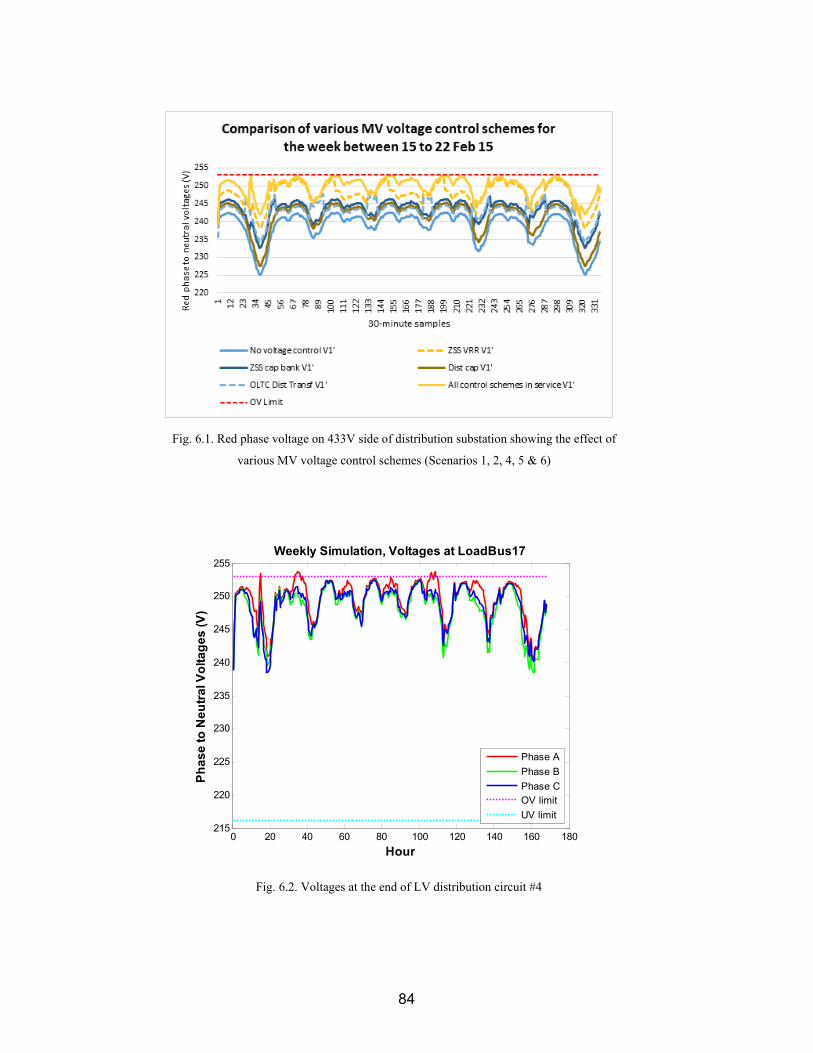
84

Fig. 6.1. Red phase voltage on 433V side of distribution substation showing the effect of

various MV voltage control schemes (Scenarios 1, 2, 4, 5 & 6)

Fig. 6.2. Voltages at the end of LV distribution circuit #4

0 20 40 60 80 100 120 140 160 180215

220

225

230

235

240

245

250

255

Hour

Ph

as

e t

o N

eu

tra

l Vo

lta

ge

s (

V)

Weekly Simulation, Voltages at LoadBus17

Phase A

Phase B

Phase COV limit

UV limit

85

Line Drop Compensation

As an alternative to setting a high base voltage to cater for peak load condition, Scenario

3 explores the use of Line Drop Compensation (LDC) to provide a dynamic voltage set

point for the SHM 66/22kV transformer OLTC control. The voltage set point is increased

in proportion to load increase to keep the delivered voltage constant at a network location,

generally the load centre of an outgoing MV feeder. In this scenario we have set the LDC

to keep the voltage at the 22kV side of Cypress-Stillia distribution substation (Bus7) at

the target value. The resultant voltage profile is shown in Figure 6.3. The voltages at the

end of LV distribution circuit (Bus17) have also improved, as can be seen in Figure 6.4.

LDC has been effective in lowering the supply voltage during light load period while

keeping the voltage at a sufficiently high level during peak load period.

A dynamic voltage regulation scheme is conceptually superior to flat voltage control as

it has the potential to optimise the voltage delivery in accordance with parameters that

affect voltage drops along the distribution circuit. In practice the application of LDC

requires careful planning when distribution feeders from the same substation are not

homogenous (from load/generation distribution and impedance characteristics

perspective). One possible approach is to supplement the LDC with local voltage control

strategies such as LV shunt capacitors and voltage regulating distribution transformers,

in accordance with the local conditions [50, 55].

Fig. 6.3. The use of Line Drop Compensation has improved the voltage at the 433V side of

the distribution substation (Bus9)

Fig. 6.4. The use of Line Drop Compensation has improved the voltage at the end of LV circuit #4 (Bus17)

0 20 40 60 80 100 120 140 160 180215

220

225

230

235

240

245

250

255

Hour

Ph

as

e t

o N

eu

tra

l Vo

lta

ge

s (

V)

Weekly Simulation, Voltages at LoadBus17

Phase A

Phase B

Phase COV limit

UV limit

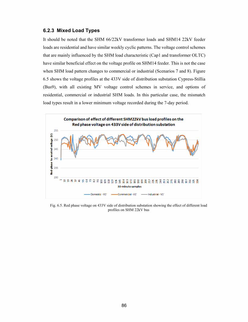
86

Mixed Load Types

It should be noted that the SHM 66/22kV transformer loads and SHM14 22kV feeder

loads are residential and have similar weekly cyclic patterns. The voltage control schemes

that are mainly influenced by the SHM load characteristic (Cap1 and transformer OLTC)

have similar beneficial effect on the voltage profile on SHM14 feeder. This is not the case

when SHM load pattern changes to commercial or industrial (Scenarios 7 and 8). Figure

6.5 shows the voltage profiles at the 433V side of distribution substation Cypress-Stillia

(Bus9), with all existing MV voltage control schemes in service, and options of

residential, commercial or industrial SHM loads. In this particular case, the mismatch

load types result in a lower minimum voltage recorded during the 7-day period.

Fig. 6.5. Red phase voltage on 433V side of distribution substation showing the effect of different load profiles on SHM 22kV bus

87

Effect of LV Voltage Regulation Control

LV Model to Include Effects of Circuit unbalance, Load Unbalance and Ground Connections

As discussed in Section 5.3, it is important to model the LV distribution network as 4-

wire (R, W, B & N) and include the Multiple Earthed Neutral (MEN) ground connections

at the customer points of connection. Figure 6.6 provides an example of the load flow

result when the network is modelled as 3-wire balanced circuit, which is very different to

that in Figure 6.2 for a 4-wire unbalanced circuit.

Fig. 6.6. Voltages at the end of LV distribution circuit #4, with MV and LV network modelled as 3-wire balanced network

0 20 40 60 80 100 120 140 160 180215

220

225

230

235

240

245

250

255

260

Hour

Ph

as

e t

o E

art

h V

olt

ag

es

(V

)

Voltages at LoadBus17 (modelled as 3-wire balanced network)

Phase A

Phase B

Phase COV limit

UV limit

88

LV PV Generation Caused Localized Voltage Rise and Voltage Unbalance

Excess generated power from a PV system will travel along the distribution network until

it is consumed by load, while raising the voltage along the way. The voltage rise is

therefore superimposed upon the network voltage. As the two PV generators in

distribution circuit #4 are all connected to the red phase, one would expect the voltage

rise effect to be more pronounced on the red phase of sparsely loaded buses. This is clearly

seen on Bus17 as shown in Figure 6.7.

As the voltage in this distribution network is already on the high side, there are occasions

during the week when the localized voltage rises have exceeded the prescribed

overvoltage limit (shown dotted in Figure 6.7). When this occurs, PV inverters can trip

on over-voltage and customer equipment may malfunction or their life span shortened.

The difference between the voltages on the three phases also gives rise to voltage

unbalance.

Phase Voltage Unbalance, Its Effect and Applicable Standards

Unbalance between the three phases in the 4-wire LV network is magnified by the

difference between loads and generations in each phase, and unbalanced phase geometry

(lack of transposition and 1/2-phase supply spurs). This results in voltage appearing on

the neutral connection (zero sequence voltage V0), and phase voltages that are different

Fig. 6.7. Voltages at the end of LV distribution circuit #4

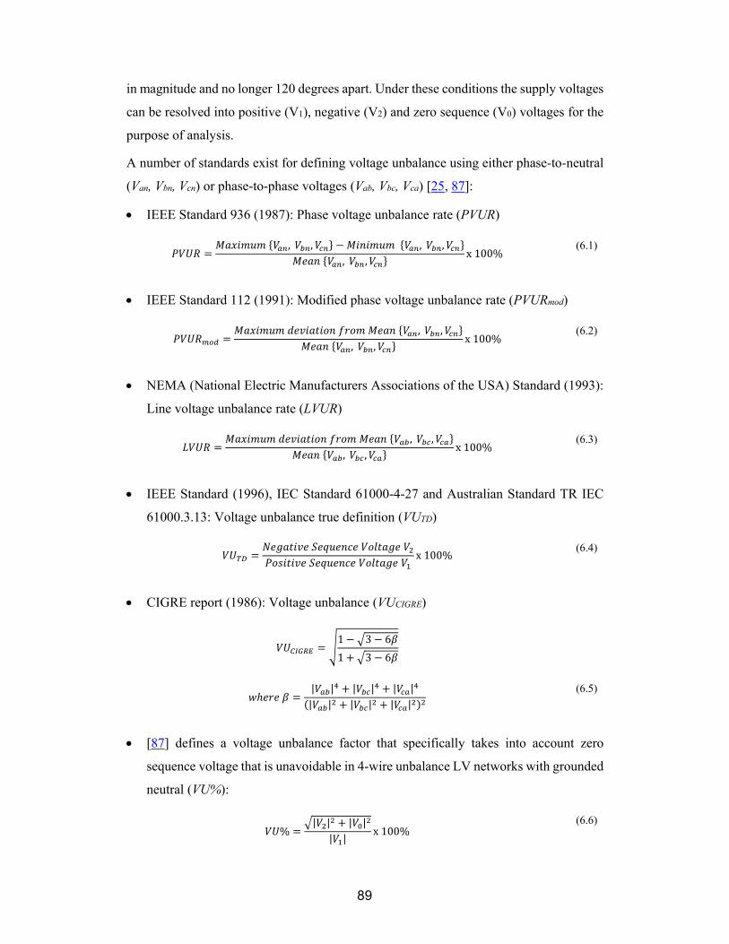
89

in magnitude and no longer 120 degrees apart. Under these conditions the supply voltages

can be resolved into positive (V1), negative (V2) and zero sequence (V0) voltages for the

purpose of analysis.

A number of standards exist for defining voltage unbalance using either phase-to-neutral

(Van, Vbn, Vcn) or phase-to-phase voltages (Vab, Vbc, Vca) [25, 87]:

IEEE Standard 936 (1987): Phase voltage unbalance rate (PVUR)

, , , ,, ,

x 100% (6.1)

IEEE Standard 112 (1991): Modified phase voltage unbalance rate (PVURmod)

, ,, ,

x 100% (6.2)

NEMA (National Electric Manufacturers Associations of the USA) Standard (1993):

Line voltage unbalance rate (LVUR)

, ,, ,

x 100% (6.3)

IEEE Standard (1996), IEC Standard 61000-4-27 and Australian Standard TR IEC

61000.3.13: Voltage unbalance true definition (VUTD)

x 100% (6.4)

CIGRE report (1986): Voltage unbalance (VUCIGRE)

1 3 6

1 3 6

| | | | | || | | | | |

(6.5)

[87] defines a voltage unbalance factor that specifically takes into account zero

sequence voltage that is unavoidable in 4-wire unbalance LV networks with grounded

neutral (VU%):

%| | | |

| |x 100%

(6.6)

90

where V1, V2 and V0 are the positive sequence, negative sequence and zero sequence

voltages respectively.

For a three-phase, four-wire LV feeder with equally sized phase and neutral conductors,

it can be shown that LVUR and VUTD are equivalent, while VU% is higher than VUTD but

lower than PVUR and PVURmod.

Negative sequence voltages affect the performance and life expectancy of customer 3-

phase equipment (such as 3-phase motors), and zero sequence currents (caused by zero

sequence voltages) affect the rating of network equipment and increase network losses

[87, 88]. In addition, the neutral voltage shift caused by zero sequence voltages will

further compound the overvoltage and undervoltage problems as it will cause one phase

voltage to go higher while the other two phases will go lower [82]. As such both the

negative and zero sequence voltages should be controlled in addition to voltage

magnitudes.

This thesis uses VU% defined by Equation 6.6 to calculate voltage unbalance on the 4-

wire LV network.

Optimal Solar Generator Placement to Reduce Voltage Unbalance

Under automatic connection policy, supply utilities do not generally select the phases for

the connection of solar generators. For customers on single-phase supply, solar generators

are connected to the same supply phase. For customers on a three-phase supply, the solar

generators are connected to the phase deemed suitable by the solar installers. The

localized voltage rise, however, will be dependent on the phases where the solar

generators are connected as well as the distribution of loads among the three phases.

Balancing loads and solar generation across all three phases will increase the capacity of

the network to accommodate more solar generators without expensive network

augmentation or implementation of new smart grid technologies. Customer loads and

solar generation, however, are stochastic in nature hence we need a methodology to

allocate loads and solar generation.

To tackle the issues of phase voltage rise and unbalance voltages, we propose that loads

and generators are allocated to the three supply phases of the LV network based on

minimizing voltage unbalance taking into account both negative and zero sequence

91

voltages, subject to the constraint that voltages on each LV supply node/bus are within

the regulated limits.

For a LV network with multiple nodes where voltage unbalance can be calculated, we

define a composite index, the network voltage unbalance factor f(x), as the average of the

weighted, maximum voltage unbalance, on each supply node/bus over the period of

simulation. This can be expressed mathematically as

1∗ VU%max n

(6.7)

The aim is to minimize f(x) subject to 216V ≤Vn ≤253V, where

(VU%max)n = maximum voltage unbalance at the nth mode over the period of simulation

Vn = voltage on the nth mode

M = number of node/bus

Wn = weight coefficient allocated to the nth mode

Wn is normally set to 1 but can be set higher for the node/bus where 3-phase customer

equipment, susceptible to voltage unbalance, have been installed.

Equation 6.7 uses the average of the weighted maximum voltage unbalance on each

supply node/bus, not the weighted maximum voltage unbalance. This is based on the

reasoning that voltage unbalance has an undesirable effect on customer equipment and

hence the voltage unbalance on all supply nodes/buses should be taken into consideration

in the optimisation effort.

The methodology is applied to the network model where there are two PV generators,

PV1 and PV2. Keeping the load allocation constant, the PV generators can each be

connected to the red, white or blue phase of the three-phase supply network, resulting in

nine combinations. For each combination, load flow calculation is carried out and voltage

unbalance determined for each LV bus using Equation 6.6. The network voltage

unbalance factor, f(x), can then be calculated using Equation 6.7. Table 6.2 summarizes

the result of the network voltage unbalance factor calculated for the nine combinations,

with Wi set to 1 for each bus. It can be seen that minimum network voltage unbalance

occurs when PV1 is connected to white phase and PV2 to blue phase. The current PV

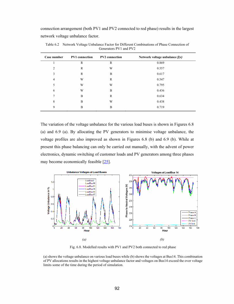
92

connection arrangement (both PV1 and PV2 connected to red phase) results in the largest

network voltage unbalance factor.

Table 6.2 Network Voltage Unbalance Factor for Different Combinations of Phase Connection of Generators PV1 and PV2

Case number PV1 connection PV2 connection Network voltage unbalance f(x)

1 R R 0.869

2 R W 0.557

3 R B 0.617

4 W R 0.547

5 W W 0.795

6 W B 0.436

7 B R 0.634

8 B W 0.438

9 B B 0.719

The variation of the voltage unbalance for the various load buses is shown in Figures 6.8

(a) and 6.9 (a). By allocating the PV generators to minimise voltage unbalance, the

voltage profiles are also improved as shown in Figures 6.8 (b) and 6.9 (b). While at

present this phase balancing can only be carried out manually, with the advent of power

electronics, dynamic switching of customer loads and PV generators among three phases

may become economically feasible [25].

(a) (b)

Fig. 6.8. Modelled results with PV1 and PV2 both connected to red phase

(a) shows the voltage unbalance on various load buses while (b) shows the voltages at Bus14. This combination of PV allocations results in the highest voltage unbalance factor and voltages on Bus14 exceed the over voltage limits some of the time during the period of simulation.

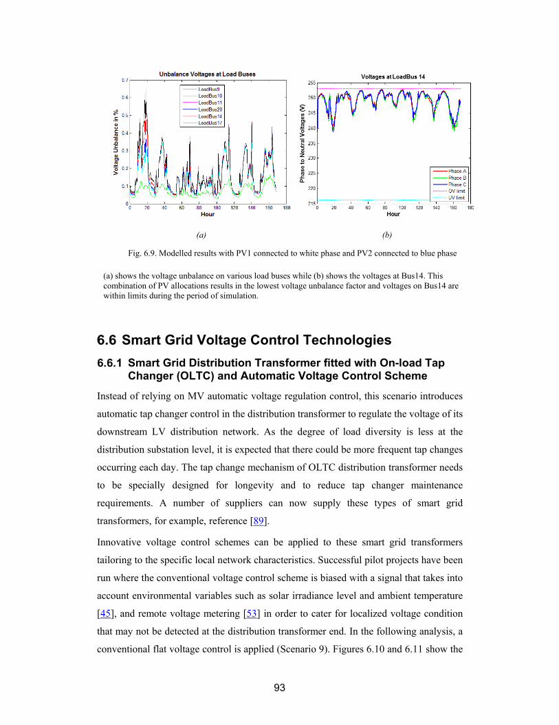
93

Smart Grid Voltage Control Technologies

Smart Grid Distribution Transformer fitted with On-load Tap Changer (OLTC) and Automatic Voltage Control Scheme

Instead of relying on MV automatic voltage regulation control, this scenario introduces

automatic tap changer control in the distribution transformer to regulate the voltage of its

downstream LV distribution network. As the degree of load diversity is less at the

distribution substation level, it is expected that there could be more frequent tap changes

occurring each day. The tap change mechanism of OLTC distribution transformer needs

to be specially designed for longevity and to reduce tap changer maintenance

requirements. A number of suppliers can now supply these types of smart grid

transformers, for example, reference [89].

Innovative voltage control schemes can be applied to these smart grid transformers

tailoring to the specific local network characteristics. Successful pilot projects have been

run where the conventional voltage control scheme is biased with a signal that takes into

account environmental variables such as solar irradiance level and ambient temperature

[45], and remote voltage metering [53] in order to cater for localized voltage condition

that may not be detected at the distribution transformer end. In the following analysis, a

conventional flat voltage control is applied (Scenario 9). Figures 6.10 and 6.11 show the

(a) (b)

Fig. 6.9. Modelled results with PV1 connected to white phase and PV2 connected to blue phase

(a) shows the voltage unbalance on various load buses while (b) shows the voltages at Bus14. This combination of PV allocations results in the lowest voltage unbalance factor and voltages on Bus14 are within limits during the period of simulation.

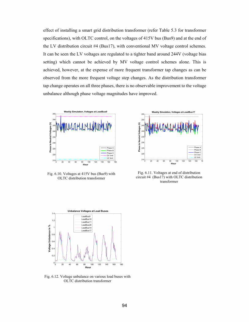
94

effect of installing a smart grid distribution transformer (refer Table 5.3 for transformer

specifications), with OLTC control, on the voltages of 415V bus (Bus9) and at the end of

the LV distribution circuit #4 (Bus17), with conventional MV voltage control schemes.

It can be seen the LV voltages are regulated to a tighter band around 244V (voltage bias

setting) which cannot be achieved by MV voltage control schemes alone. This is

achieved, however, at the expense of more frequent transformer tap changes as can be

observed from the more frequent voltage step changes. As the distribution transformer

tap change operates on all three phases, there is no observable improvement to the voltage

unbalance although phase voltage magnitudes have improved.

Fig. 6.12. Voltage unbalance on various load buses with OLTC distribution transformer

0 20 40 60 80 100 120 140 160 1800

0.2

0.4

0.6

0.8

1

1.2

1.4

Hour

Vo

lta

ge

Un

ba

lan

ce

in %

Unbalance Voltages at Load Buses

LoadBus9LoadBus10

LoadBus11

LoadBus20

LoadBus14LoadBus17

Fig. 6.10. Voltages at 415V bus (Bus9) with OLTC distribution transformer

0 20 40 60 80 100 120 140 160 180215

220

225

230

235

240

245

250

255

Hour

Ph

as

e t

o N

eu

tra

l Vo

lta

ge

s (

V)

Weekly Simulation, Voltages at LoadBus9

Phase A

Phase B

Phase COV limit

UV limit

Fig. 6.11. Voltages at end of distribution circuit #4 (Bus17) with OLTC distribution

transformer

0 20 40 60 80 100 120 140 160 180215

220

225

230

235

240

245

250

255

Hour

Ph

as

e t

o N

eu

tra

l Vo

lta

ge

s (

V)

Weekly Simulation, Voltages at LoadBus17

Phase A

Phase B

Phase COV limit

UV limit

95

Smart PV Inverters

Up to now we have considered voltage control technologies that affect all three phases of

the supply network and cannot directly mitigate the effect of PV generators that are

connected to one phase. Smart PV inverters are now commercially available which act to

limit the effect of PV generators on the phase(s) of the network they connect to. In some

designs the smart inverter can even assist with optimizing voltage delivery by acting in a

manner similar to a Distribution Static Compensator (DSTATCOM).

A number of smart inverter control algorithms are commercially available: Volt-Watt (V-

W), Volt-Var (V-V) and fixed power factor (PF) [48]. In PF control, the fixed power

factor is generally set to a value such that the PV system appears slightly inductive to the

grid. As the PV generates active power, the inverter acts to absorb reactive power from

the grid in proportion to the active power output. In V-W control, the active power output

of the inverter will be curtailed when the voltage is high. In V-V control, the smart inverter

is set to absorb reactive power (Var) when the voltage is high, and generate reactive power

when the voltage is low. A special use of V-V control is to absorb/generate reactive power

to assist with voltage delivery even when the inverter is not outputting active power e.g.

after the sun sets. [45] shows that dynamic power control methods such as V-W and V-V

provide superior results compared with static reactive power control methods such as PF.

The simulations are therefore performed with V-W and V-V control. In the absence of

internationally accepted standard for the inverter control characteristics, the

characteristics used in the simulation are chosen to demonstrate beneficial effect on

voltage outcome.

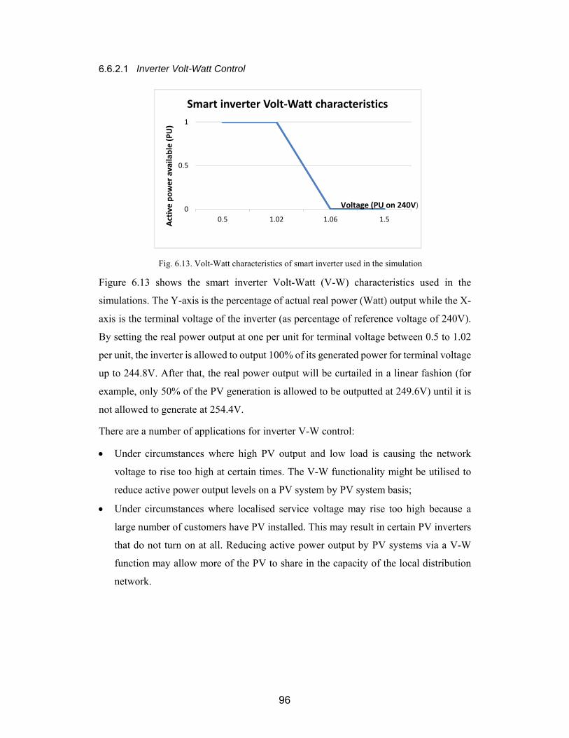
96

Inverter Volt-Watt Control

Figure 6.13 shows the smart inverter Volt-Watt (V-W) characteristics used in the

simulations. The Y-axis is the percentage of actual real power (Watt) output while the X-

axis is the terminal voltage of the inverter (as percentage of reference voltage of 240V).

By setting the real power output at one per unit for terminal voltage between 0.5 to 1.02

per unit, the inverter is allowed to output 100% of its generated power for terminal voltage

up to 244.8V. After that, the real power output will be curtailed in a linear fashion (for

example, only 50% of the PV generation is allowed to be outputted at 249.6V) until it is

not allowed to generate at 254.4V.

There are a number of applications for inverter V-W control:

Under circumstances where high PV output and low load is causing the network

voltage to rise too high at certain times. The V-W functionality might be utilised to

reduce active power output levels on a PV system by PV system basis;

Under circumstances where localised service voltage may rise too high because a

large number of customers have PV installed. This may result in certain PV inverters

that do not turn on at all. Reducing active power output by PV systems via a V-W

function may allow more of the PV to share in the capacity of the local distribution

network.

Fig. 6.13. Volt-Watt characteristics of smart inverter used in the simulation

0

0.5

1

0.5 1.02 1.06 1.5

Active power available (PU)

Voltage (PU on 240V)

Smart inverter Volt‐Watt characteristics 

97

The effect of V-W control on the two PV generators connected to the red phase can be

seen in Figure 6.14. The occurrences of red phase voltage rise above regulatory limit have

been corrected with the V-W control. As seen in Figure 6.15, voltage unbalance has also

been improved.

Inverter Volt-Var Control

With Volt-Var (V-V) control, reactive power is generated or absorbed depending on the

terminal voltage of the inverter. The amount of reactive power output is a percentage of

(a) (b)

Fig. 6.14. Effect of Smart Inverter Volt-Watt control on phase voltages

(a) No smart inverter control

(b) PV1 and PV2 are fitted with smart inverters with Volt-Watt control as per Fig.6.13

(a) (b)

Fig. 6.15. Effect of Smart Inverter Volt-Watt control on voltage unbalance

(a) No smart inverter control

(b) PV1 and PV2 are fitted with smart inverters with Volt-Watt control as per Fig.6.13 characteristics

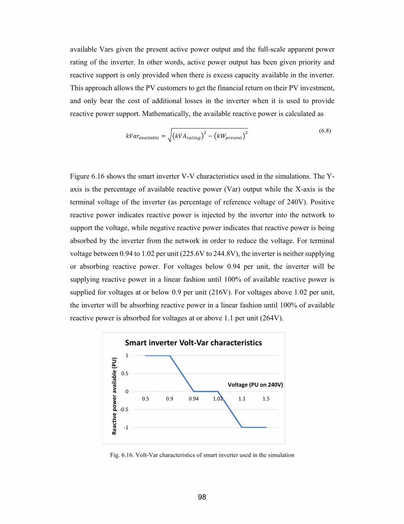
98

available Vars given the present active power output and the full-scale apparent power

rating of the inverter. In other words, active power output has been given priority and

reactive support is only provided when there is excess capacity available in the inverter.

This approach allows the PV customers to get the financial return on their PV investment,

and only bear the cost of additional losses in the inverter when it is used to provide

reactive power support. Mathematically, the available reactive power is calculated as

(6.8)

Figure 6.16 shows the smart inverter V-V characteristics used in the simulations. The Y-

axis is the percentage of available reactive power (Var) output while the X-axis is the

terminal voltage of the inverter (as percentage of reference voltage of 240V). Positive

reactive power indicates reactive power is injected by the inverter into the network to

support the voltage, while negative reactive power indicates that reactive power is being

absorbed by the inverter from the network in order to reduce the voltage. For terminal

voltage between 0.94 to 1.02 per unit (225.6V to 244.8V), the inverter is neither supplying

or absorbing reactive power. For voltages below 0.94 per unit, the inverter will be

supplying reactive power in a linear fashion until 100% of available reactive power is

supplied for voltages at or below 0.9 per unit (216V). For voltages above 1.02 per unit,

the inverter will be absorbing reactive power in a linear fashion until 100% of available

reactive power is absorbed for voltages at or above 1.1 per unit (264V).

Fig. 6.16. Volt-Var characteristics of smart inverter used in the simulation

‐1

‐0.5

0

0.5

1

0.5 0.9 0.94 1.02 1.1 1.5

Reactive

 power available (PU)

Voltage (PU on 240V)

Smart inverter Volt‐Var characteristics 

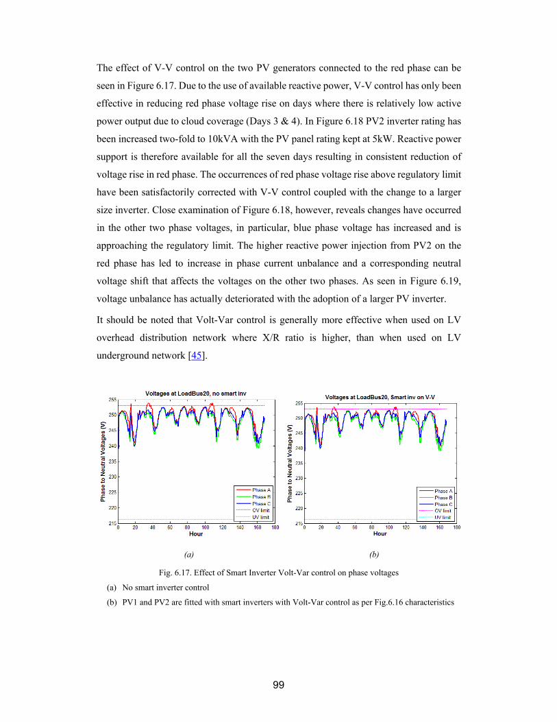
99

The effect of V-V control on the two PV generators connected to the red phase can be

seen in Figure 6.17. Due to the use of available reactive power, V-V control has only been

effective in reducing red phase voltage rise on days where there is relatively low active

power output due to cloud coverage (Days 3 & 4). In Figure 6.18 PV2 inverter rating has

been increased two-fold to 10kVA with the PV panel rating kept at 5kW. Reactive power

support is therefore available for all the seven days resulting in consistent reduction of

voltage rise in red phase. The occurrences of red phase voltage rise above regulatory limit

have been satisfactorily corrected with V-V control coupled with the change to a larger

size inverter. Close examination of Figure 6.18, however, reveals changes have occurred

in the other two phase voltages, in particular, blue phase voltage has increased and is

approaching the regulatory limit. The higher reactive power injection from PV2 on the

red phase has led to increase in phase current unbalance and a corresponding neutral

voltage shift that affects the voltages on the other two phases. As seen in Figure 6.19,

voltage unbalance has actually deteriorated with the adoption of a larger PV inverter.

It should be noted that Volt-Var control is generally more effective when used on LV

overhead distribution network where X/R ratio is higher, than when used on LV

underground network [45].

(a) (b)

Fig. 6.17. Effect of Smart Inverter Volt-Var control on phase voltages

(a) No smart inverter control

(b) PV1 and PV2 are fitted with smart inverters with Volt-Var control as per Fig.6.16 characteristics

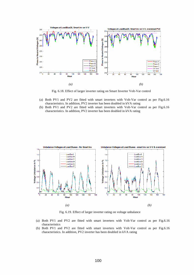
100

(a) (b)

Fig. 6.18. Effect of larger inverter rating on Smart Inverter Volt-Var control

(a) Both PV1 and PV2 are fitted with smart inverters with Volt-Var control as per Fig.6.16

characteristics. In addition, PV2 inverter has been doubled in kVA rating

(b) Both PV1 and PV2 are fitted with smart inverters with Volt-Var control as per Fig.6.16

characteristics. In addition, PV2 inverter has been doubled in kVA rating

(a) (b)

Fig. 6.19. Effect of larger inverter rating on voltage unbalance

(a) Both PV1 and PV2 are fitted with smart inverters with Volt-Var control as per Fig.6.16

characteristics

(b) Both PV1 and PV2 are fitted with smart inverters with Volt-Var control as per Fig.6.16

characteristics. In addition, PV2 inverter has been doubled in kVA rating

101

Connect Battery Storage to PV Generator

The effect of localized voltage rise caused by excess PV generation could be overcome if

the excess generation is used to charge up a local battery. The stored energy can then be

used to reduce the evening peak demand. This option has become economically feasible

due to the reduction in battery cost and the continual rise in price of electricity in many

parts of the world. Similar rationales have been applied to other forms of controllable

loads such as water heating and space heating to absorb excess PV generation [52].

Battery storage control algorithms

The ideal charging strategy of a storage battery is to direct all surplus generated power

(solar generation minus local consumption) to the battery. The stored energy is then

discharged at the appropriate times (generally during peak times) in line with the cost of

electricity stipulated in the tariff. Battery controllers to achieve this ideal characteristics

will be, by necessity, rather complex due to the need to monitor the PV generation and to

provide accurate short-term forecast of load consumption, all in near real-time. Research

into the ideal battery control algorithms is outside the scope of this thesis.

In order to illustrate the concept of using battery storage to manage voltage rise, we have

modelled a 4.4kW/25kWh battery installed by Customer 7 who has a 5kW PV generator

(PV2). The rather odd figure of 4.4kW is arrived at based on a 4kW battery with a 90%

energy conversion efficiency. We have adopted a charge/discharge characteristics (Figure

6.20) where charging occurs at a rate determined by the loadshape of the solar irradiance

(hence tracking closely with the loadshape of PV generation), followed by discharging at

a rate of the customer load usage from 6pm onwards.

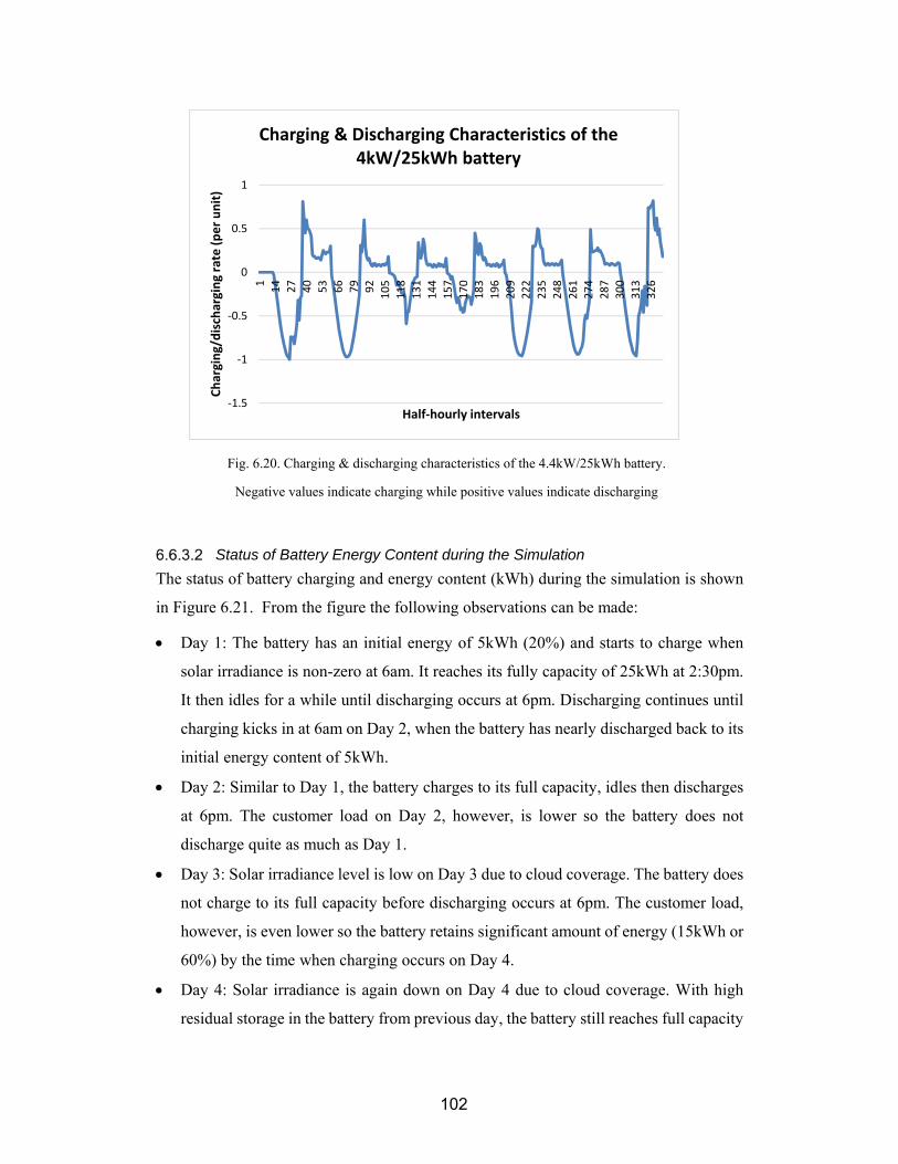
102

Status of Battery Energy Content during the Simulation

The status of battery charging and energy content (kWh) during the simulation is shown

in Figure 6.21. From the figure the following observations can be made:

Day 1: The battery has an initial energy of 5kWh (20%) and starts to charge when

solar irradiance is non-zero at 6am. It reaches its fully capacity of 25kWh at 2:30pm.

It then idles for a while until discharging occurs at 6pm. Discharging continues until

charging kicks in at 6am on Day 2, when the battery has nearly discharged back to its

initial energy content of 5kWh.

Day 2: Similar to Day 1, the battery charges to its full capacity, idles then discharges

at 6pm. The customer load on Day 2, however, is lower so the battery does not

discharge quite as much as Day 1.

Day 3: Solar irradiance level is low on Day 3 due to cloud coverage. The battery does

not charge to its full capacity before discharging occurs at 6pm. The customer load,

however, is even lower so the battery retains significant amount of energy (15kWh or

60%) by the time when charging occurs on Day 4.

Day 4: Solar irradiance is again down on Day 4 due to cloud coverage. With high

residual storage in the battery from previous day, the battery still reaches full capacity

Fig. 6.20. Charging & discharging characteristics of the 4.4kW/25kWh battery.

Negative values indicate charging while positive values indicate discharging

‐1.5

‐1

‐0.5

0

0.5

1

1

14

27

40

53

66

79

92

105

118

131

144

157

170

183

196

209

222

235

248

261

274

287

300

313

326

Charging/discharging rate (per unit) 

Half‐hourly intervals

Charging & Discharging Characteristics of the 4kW/25kWh battery

103

by the time when discharging occurs at 6pm. The load is low so the battery retains

significant amount of storage (~15kWh) when charging occurs on Day 5.

Day 5: Solar irradiance is back to the normal high level. The battery is no longer able

to absorb most of the PV output due to the initial energy content. We start to see the

lengthening of the idle period where the battery is fully charged.

Day 6 and Day 7: similar to Day 5.

Effect of Battery on Voltage Rise

The effect of the battery storage on the voltage profile of Bus20 can be seen by comparing

Figure 6.22 and Figure 6.23. Red phase overvoltage caused by PV2 generating has been

reduced while the red phase voltage during peak load has improved. The voltages are now

within regulatory limit except on Day 5 where there are still excursions over the limit.

This is due to the battery reaching its full capacity and no longer able to absorb excess

PV generation as described in 6.6.3.2. Voltage unbalance improves during the period

when the battery is absorbing PV generation but deteriorates when the battery discharges.

Overall there is a small improvement in voltage unbalance factor (Figure 6.24).

Fig. 6.21. Battery energy and charging status during the simulation.

Note State =-1 when charging, =0 when idle, =+1 when discharging

‐5

0

5

10

15

20

25

30

1

17

33

49

65

81

97

113

129

145

161

177

193

209

225

241

257

273

289

305

321Battery Energy & Charging Status 

30‐minute time interval

Storage battery energy and charging status

 kWh

State

104

Future Scenario of Higher PV Penetration

The distribution circuit has eight customers and two PV installations representing a PV

penetration of 25%. Simulation studies show that the approach of optimal PV placement

to the supply phases has been effective in ensuring the supply voltages are within the

regulatory limits on all the load buses. Now consider the additional installation of two PV

generators of 4kW each (PV3 and PV4) brining the PV penetration to 50% of customers.

One of the worst case scenarios is the new PV generators are installed by the two single-

phase customers (Customer 2 and Customer 6) as there are no choices in the phase

connection. The voltage profile on the loadbuses is now over the voltage limit with the

PV phase connection that is deemed to be optimal for the 2-PV case (Figure 6.25). The

optimal generator placement study as detailed in Section 6.5 is repeated for the two

existing PV generators (PV1 and PV2). The simulation study indicates that the

Fig. 6.22. Voltages at Bus20 without storage

battery

Fig. 6.23. Voltages at Bus20 with storage

battery

Fig. 6.24. Voltage unbalance on the load buses

with storage battery

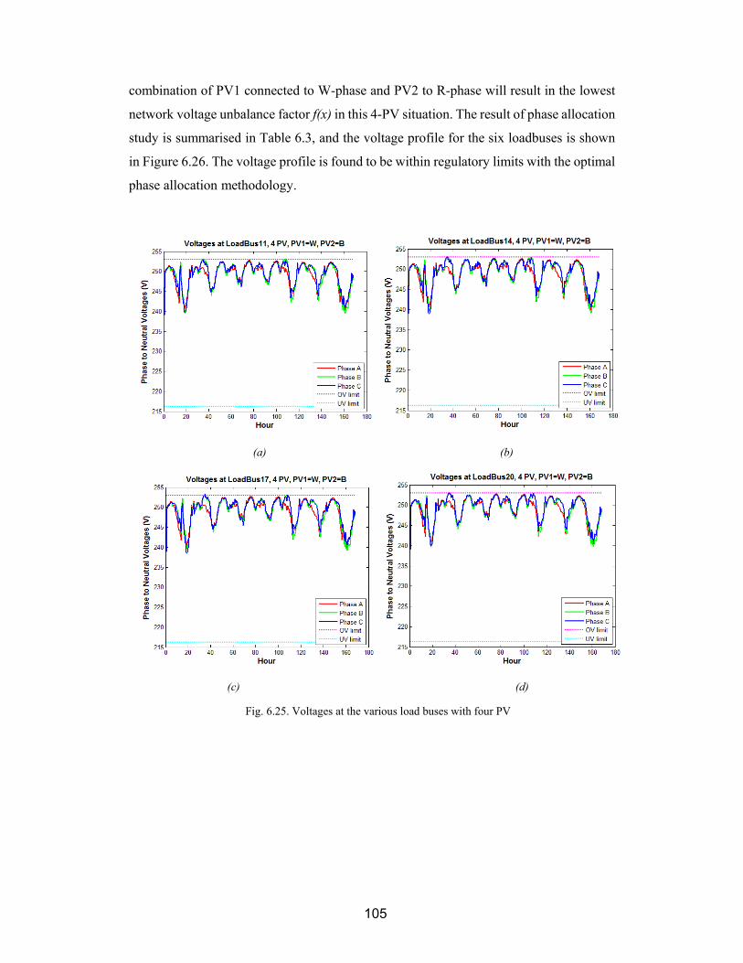
105

combination of PV1 connected to W-phase and PV2 to R-phase will result in the lowest

network voltage unbalance factor f(x) in this 4-PV situation. The result of phase allocation

study is summarised in Table 6.3, and the voltage profile for the six loadbuses is shown

in Figure 6.26. The voltage profile is found to be within regulatory limits with the optimal

phase allocation methodology.

(a) (b)

(c) (d)

Fig. 6.25. Voltages at the various load buses with four PV

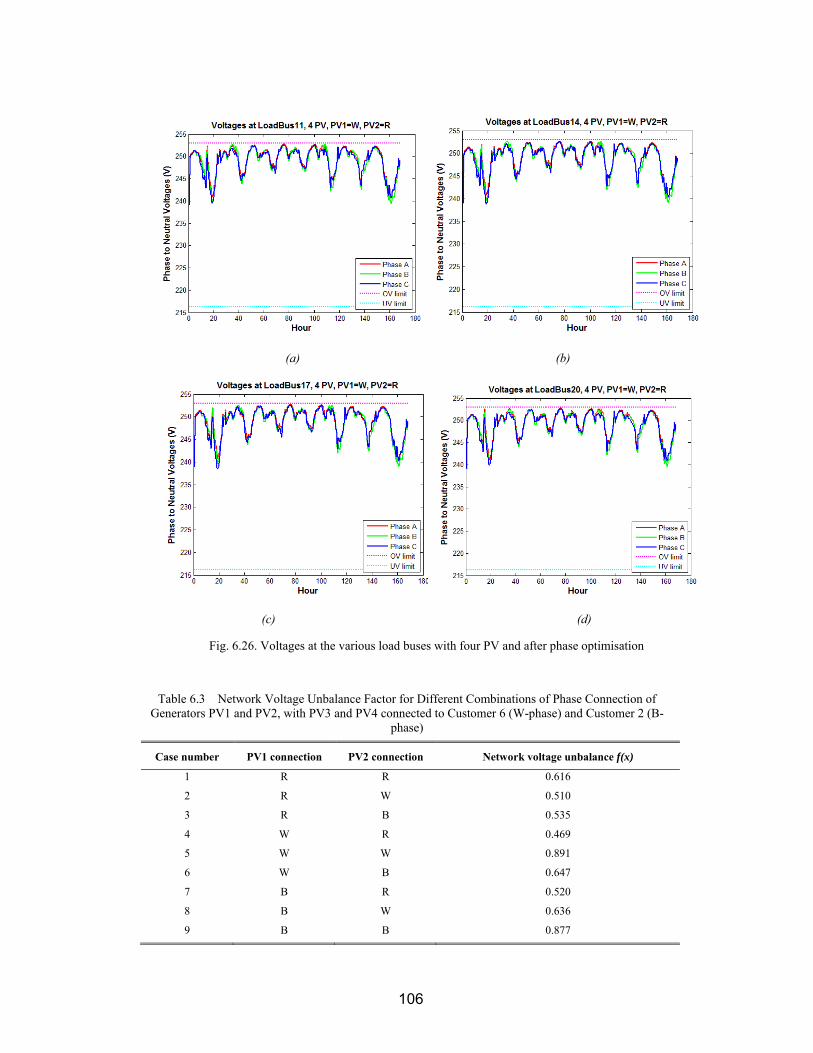
106

Table 6.3 Network Voltage Unbalance Factor for Different Combinations of Phase Connection of Generators PV1 and PV2, with PV3 and PV4 connected to Customer 6 (W-phase) and Customer 2 (B-

phase)

Case number PV1 connection PV2 connection Network voltage unbalance f(x)

1 R R 0.616

2 R W 0.510

3 R B 0.535

4 W R 0.469

5 W W 0.891

6 W B 0.647

7 B R 0.520

8 B W 0.636

9 B B 0.877

(a) (b)

(c) (d)

Fig. 6.26. Voltages at the various load buses with four PV and after phase optimisation

107

Lowering the nominal supply voltage will also be effective in reducing the risk of

localised voltage rise above the overvoltage limit. Figure 6.27 shows that the use of LDC

in this 4-PV case brings the voltage profile within regulatory limit without the need to re-

connect PV1 and PV2 to different phases. The voltage unbalance, however, is increased.

(a) (b)

(c) (d)

Fig. 6.27. Voltages at the various load buses with four PV and after phase optimisation and application of

LDC

108

Summary

The establishment of an accurate LV network model provides a good foundation for

carrying out computer simulation studies of voltage rise caused by embedded PV

generators. As residential roof-top PV generators are generally single-phase, the voltage

rise caused by the generators affect the three phases differently. Voltage unbalance also

arises and can affect customer three-phase equipment. These effects are most pronounced

on sparsely loaded lines farthest away from the supply source (i.e. the distribution

transformer).

Automatic voltage regulation control schemes applied at MV network are traditionally

biased to deliver a supply voltage that is at the high end of the allowable voltage range,

to cater for large voltage drop at peak load conditions. The voltage bias leaves little

headroom for the local voltage rise caused by excess PV generation. The simulation

results indicate that dynamic voltage control schemes should be considered for MV

voltage regulation to lower the supply voltage under light load conditions. Improvement

to MV voltage regulation control will improve the hosting capacity of the LV network

for embedded PV generators. It is, however, ineffective in addressing the phase

discrepancy caused by the mismatch of PV generation and load on the three supply

phases.

To address the effect of PV generation on different phases of the supply network, an

operational approach can be taken to identify the optimal phase connection of the PV

generators that will result in the lowest voltage unbalance. The thesis proposes an

allocation methodology based on minimising the network voltage unbalance factor, and

demonstrate the beneficial effect of such an approach in the simulation results.

Investing in smart grid technologies will further increase the hosting capacity of the LV

network for embedded PV generators. The thesis has studied and demonstrated the

beneficial effects of on-load tap changing distribution transformer, smart inverters with

Volt-Watt and Volt-Var control, and battery storage. Careful planning in the selection of

control characteristics and battery size, however, is required so these smart grid

technologies can deliver the benefits as modelled.

109

Chapter 7 - Conclusions and

Future Research

Overview

This chapter draws an overarching commentary of the dissertation including the research

undertaken and the subsequent findings. Section 7.2 provides an overall conclusion and

outlines the main findings of this thesis. Section 7.3 closes the thesis with

recommendations for future research directions.

Conclusions

The aim of this thesis is to identify practical, cost effective measures that can be taken by

supply utilities to accommodate the increasing penetration of grid connected, residential

roof-top photo-voltaic generation systems. It achieves its purpose by firstly examining

the present status of voltage quality delivered to LV customers and identifying the effect

of PV on voltage quality. The work is then followed by establishing accurate PV generator

and LV network models. Computer simulation studies are then performed on network

model based on data of a realistic LV network. Various scenarios are simulated using

existing voltage control schemes, new proposed planning approach and smart grid

technologies, and their effect on voltage quality examined. The research is enabled by the

availability of voltage quality data from smart meters that have been rolled out to all

residential customers.

The main results and research contributions of this thesis can be summarised as follows:

1. Gaining a deeper insight of voltage quality delivered to end customers:

By performing exploratory analysis of overvoltage and undervoltage event

data measured by approximately 100,000 smart meters over a 6-day period, a

picture emerges that a significant number of customers have either

experienced overvoltage (>12%) or undervoltage (>6%) during the period.

Undervoltage events are found to be temperature dependent and occur only

occasionally during hot days (>30oC maximum ambient temperature).

Overvoltage events, however, are common occurrences. This result highlights

the inadequacy of the existing voltage control schemes.

110

By providing an electrical connectivity overlay to the overvoltage and

undervoltage sites, upstream distribution substations and zone substations can

be identified and targeted for more detailed voltage quality investigation.

The exploratory data analysis also finds that higher percentage of customer

sites, with roof-top PV installations, have overvoltage events starting between

8am to 2pm than non-PV sites. On a macro level this indicates that PV

generation has most likely contributed to the occurrence of overvoltage

events.

Usefulness of the current smart meter voltage quality data can be improved by

the provision of time series data of voltage, current and power factor.

Resolution of the time series data would be limited by the available bandwidth

of the 2-way meter communication system but 5-minute data appears to be

adequate for most applications.

2. Developing a practical roof-top PV generator model that can be used in computer

simulation studies by distribution utilities:

PV generator output varies within the day, between seasons, is affected by

environmental variables of ambient temperature and clearness of sky, and the

orientation of the PV panel. Taking the nameplate rating as a PV generator

output is not a correct representation in computer simulations.

Accurate silicon based PV generator models can be developed using a

component approach, starting with Stockley’s diode equations for the p-n

junction building up to a model for individual PV cell output, followed by

models for the dc/ac inverter, and solar irradiance modelling. The data

required for these models are extensive and difficult to acquire for small roof-

top PV generators that are generally subjected to a streamline connection

process.

By treating the PV as a generation system, a simplified mathematical model

linking time-varying inputs (ambient temperature, global solar irradiance) to

electrical output has been established. Practicality of the model is further

guaranteed through the analysis that demonstrates the use of global solar

irradiance recorded at a nearby weather station as proxy for the irradiance

measured at the PV panel. The accuracy of the simplified model was verified

using smart meter data.

111

The PV generator model can be used in a number of applications, including

its use in computer simulations to study the effect PV generator on voltage

quality.

3. Developing a network model for a 4-wire unbalanced LV distribution circuit

A traditional lack of priority and focus means distribution utilities do not have

the data required to set up an accurate LV network model. This has severely

limited the capability of distribution utilities to adapt to the evolving needs of

customers. In the case of roof-top PV penetration, the lack of modelling

capability means most utilities do not have a clear understanding of the impact

of these PV generators. They are likely to adopt a conservative approach

which will unnecessarily limit the penetration of these customer installations.

The network sensing functions incorporated in modern smart meters have

enabled distribution utilities to establish LV network parameters such as

customer phase connection, supply impedance and to detect network

abnormalities through big data analytics.

Due to the unbalanced nature of the LV 4-wire distribution network caused by

the lack of phase transposition, phase-to-neutral load/generator connections

and current flows in the neutral conductor and earth, we cannot apply directly

the simple line/cable impedance data supplied by manufacturers. The thesis

adopts the approach to calculate line impedances using the Carson’s

equations. Carson assumes the earth is an infinite, uniform solid with a flat

uniform upper surface and a constant resistivity. The equations of self and

mutual impedances made use of conductor images; that is, every conductor at

a given distance above ground has an image conductor the same distance

below ground. Carson’s equations therefore require details about the physical

construction of the distribution circuit (phase conductor spacing, distance of

conductors above ground), conductor construction details (conductor radius)

as well as resistance and inductance data.

A distribution network model, based on a real LV distribution circuit in

Jemena Electricity Networks, is set up using load data from Supervisory

Control and Data Acquisition (SCADA) system and smart meters, line

impedance data using Carson’s equations, with explicit modelling of the

112

neutral conductors and Multiple Earthed Neutral (MEN) system, and

embedded PV generators.

The network model is set up in OpenDSSTM, an open-source electrical system

simulation tool for utility distribution systems. MATLAB© is used to drive

the OpenDSS through an in-process Component Object Model (COM)

interface for load flow simulations and result analysis.

4. Simulating the effect of existing voltage control schemes

This thesis has already identified, through exploratory analysis of smart meter

data, that voltage supplied to LV customers tends to be at the high end of the

allowable range most of the time. It has also identified that PV generators

contribute to overvoltage issues experienced by LV customers. By applying

the existing voltage control schemes and control settings to the network

model, the same result of high voltage is observed from load flow simulations.

In addition, there is voltage rise on the red phase where the two PV generators

are connected, compared with the other two phases. The combination of high

base voltage and further voltage rise caused by PV generation results in

instances of voltage non-compliance.

This thesis considered the scenario of applying Line Drop Compensation to

provide a dynamic voltage control set point that varies based on line loading.

This has the effect of lowering the voltage received by the customers during

light load period and only raising the voltage when the load is high. This

approach produces the desirable effect of lowering the base voltage so voltage

rise caused by PV generation does not result in voltage non-compliance.

Voltage unbalance caused by the mismatch of generation and load on the three

phases, however, is not addressed as existing voltage control schemes act on

all three phases and cannot correct single-phase issues.

5. Planning approach to address voltage unbalance issues

Voltage unbalance often has a detrimental effect on customer 3-phase

equipment. In addition, single-phase loads/PV generation in a three-phase,

four-wire LV network with earthed neutral gives rise to neutral voltage shift

which compounds the overvoltage and undervoltage issues. The thesis

considers modifying the existing planning approach to optimize the phase

connection of PV generators.

113

This thesis uses the definition of voltage unbalance (VU%) that incorporates

both positive, negative and zero sequence voltages, and calculate VU% for

each LV load bus during the load flow simulations. This thesis defines a

Network Voltage Unbalance Factor f(x) that takes into account the maximum

value of VU% for each load bus, and sets the objective of minimizing f(x) by

judicious placement of the PV generators to the three supply phases. The

thesis demonstrates that the approach is successful in reducing the voltage rise

caused by PV generation to within the regulatory limits even though the same

high base voltage is supplied. A hypothetical future case of adding two

additional PV generators to the distribution circuit, raising the PV penetration

to 50% of customers, is simulated. It is found that the optimal PV phase

allocation approach can still contain the voltage rise to within regulatory limits

in this high PV penetration scenario.

6. Simulating the effect of smart grid technologies

Many smart grid technologies have been proposed to address the impact of

embedded PV generation. OpenDSS provides a library of power delivery

elements that include transformers, PV generators and battery storage. Control

elements are modelled separately from the power delivery elements including

smart PV inverter control, regulator control and storage control. By combining

power delivery elements with the appropriate control elements (and control

settings), the effect of smart grid technologies on voltage rise/voltage

unbalance caused by PV generators was simulated.

By combining a transformer element with an on-load tap changer control and

using transformer specification from a supplier of smart grid transformers, this

thesis establishes the scenario of adopting an on-load tap changing distribution

transformer. The simulation result indicates that by extending automatic

voltage control into the distribution network, the voltage delivered to the

customers can be tailored to the local requirements rather than determined by

the load characteristics of the upstream zone substation and the voltage drops

on the MV network.

By combining PV generators with smart inverter control, the thesis has

demonstrated the effect of smart inverter Volt-Watt and Volt-Var controls on

voltage rise. Volt-Watt control has the effect of curtailing the active power

114

output of the PV generator when the inverter terminal voltage becomes too

high. Volt-Var control enables the PV inverter to absorb reactive power when

the voltage is high, and supply reactive power when the voltage is low. Both

smart inverter technologies are effective in reducing the voltage rise caused

by PV generation to within regulatory limits.

By fitting a battery storage element to the same premises where a PV generator

is installed and applying a control strategy for the battery to absorb excess PV

generated power and release the stored energy later during peak load period,

the thesis has demonstrated the beneficial effect of the battery storage in

reducing the voltage rise during PV generation and improving the voltage drop

during the subsequent peak load period.

7. Providing recommendations to distribution utilities

There is a pressing need to find practical, cost effective solutions that can be

deployed by supply utilities to accommodate the increasing penetration of

customer roof-top PV systems.

Modifications to existing voltage regulation schemes will be required to lower

the nominal voltage delivered to customers, as the current bias of high supply

voltage does not leave much headroom for voltage rise caused by embedded

PV generators. A relatively new Australian Standard, AS 61000.3.100 “Limits

– Steady-state voltage limits in public electricity systems”, recommends that

a sub-range of 230V +6%/-2% be used for planning purposes, instead of the

full range of 230V+10%/-6%. This approach effectively leaves an “upper

operating range” to assist the network with the absorption of embedded

generation while also providing a “lower operating range” to assist with the

network supply of heavy peak loads [90]. To achieve this objective, it is likely

that a dynamic voltage control scheme is required.

In addition, an effective method of dealing with voltage rise is to minimise

voltage unbalance between supply phases in the LV supply network. This can

be achieved by minimising the Network Voltage Unbalance Factor through

judicious placement of PV generation to the appropriate supply phases.

Central to the above proposals does require the establishment of an accurate

network model that can be used to simulate the effect of different voltage

regulation schemes and PV generator phase allocation. Utilities generally have

115

good computer models for their MV networks but LV network models are not

commonly found. As disruptions to the network are primarily occurring on the

LV network, the development of accurate LV network models should be a

priority for utilities.

Industry research is mostly focused on the development of smart grid

technologies as mitigating measures which generally require significant

additional grid investment. While transforming the supply grid performance

by investing in smart grid technologies is unavoidable, customers are already

financially burdened by the transition to a renewable energy future caused by

initiatives such as feed-in tariffs. A prioritised approach of improving existing

operational practices and implementation of smart grid technologies will help

to spread the additional investment cost over a longer time horizon.

Future Work and Recommendation

After the study into intelligent distribution voltage control in the presence of intermittent

embedded PV generation, there are other aspects of voltage control that can be

investigated further. A few possible future research directions are suggested below:

1. Electric vehicles

Electric vehicles are increasing in popularity and will present both challenges and

opportunities to the LV electricity network. The additional charging load will impact

voltage quality in particular issues relating to undervoltage and voltage unbalance.

Electric vehicles are also sources of energy storage. With controlled charging the

energy storage capacity could be used to manage excess PV generation. The

intelligent distribution voltage control investigated can be expanded to include

electric vehicle charging while optimising the network’s hosting capacity for PV

generation.

2. Modelling of other smart grid technologies

Smart grid technologies modelled in the study include on-load tap changing

distribution transformers, smart inverters and storage batteries. The study does not

attempt to investigate the effect of different control characteristics of these smart grid

technologies and this can form the basis of future research work. In addition, there is

an emerging list of smart grid technologies that promise better control of the

electricity distribution networks. Developing appropriate models of these emerging

116

technologies and their control characteristics will allow their effect to be assessed in

computer simulation studies.

3. Automate the production of network models from asset data and spatial

characteristics stored in utilities’ Geographical Information Systems (GIS) to allow

statistically valid conclusions be drawn based on a large number of simulation

studies

In this study the production of network model has been a labour-intensive process. It

is conceivable that the process can be automated beginning with the extraction of asset

data (such as line construction details) and spatial characteristics (line length, line

route, supply points) from the Geographical Information System into tabular format.

Matching of supply points with customer meter numbers create the links between

customer load information and supply points.

A simple LV distribution circuit has been modelled in the study to demonstrate the

principle of various voltage control techniques. The effectiveness of the proposed

approach in improving PV hosting capacity can be statistically determined when a

representative sample of LV distribution circuits are used in further simulation

studies. This can be undertaken when an efficient way of producing network models

can be found through process automation as above.

4. Dynamic MV voltage regulation schemes

The thesis found that dynamic voltage set points, when applied to MV voltage

regulation schemes, could improve voltage delivery to LV customers. Performance

of Line Drop Compensation scheme, however, is affected by non-homogeneity of the

MV feeders supplied by the same LDC scheme. Further research work on dynamic

MV voltage regulation schemes will be useful.

Concluding Remarks

In brief, a change of customer attitude and the emergence of affordable customer

technologies have necessitated a change in the way utility engineers design and operate

the electricity distribution networks. In the area of roof-top photo-voltaic generation

systems, Australia has topped the world in the penetration of such systems on a per capita

basis. Voltage quality issues, in particular steady-state overvoltages and voltage

unbalances, have been on the rise. To remain relevant to electricity customers, utilities

have no option but to investigate how the existing voltage controls can be improved to

117

cater for these PV generators. Improvement strategies need to be prioritised to contain

additional expenditure.

118

Appendices – OpenDSS & MatLab

Codes

OpenDSS codes for network model !Weeklypowerflow15to21Feb15!V19:reviseddisttransftomatch5‐taptransformerscommonlyfoundinJEN,increasehighvoltagefeederlengthfrom100mto1000mpersection!V20:revisedalgorithmsforstoragebattery,volt‐varandvolt‐wattcontrol;revisedLinecodes!V22:addedcommercialandindustrialloadprofiles!V23:ChangedO/HlinestogeometrytoallowCarson'sEquationtobeused!V23a:Updatednomenclatureofcircuitelementsinaccordancewithmodelschematic!V23b:versiontobeusedinconjuctionwithMATLABClearNewCircuit.SHM14EditVsource.SourceBasekV=66pu=1.015ISC3=7100ISC1=4000!TheSHMtransformershouldbemodelledaswye/delta/wye.Howevertosimplifymodellingthetransformerhasbeenmodelledasdelta/wye.NewTransformer.TR_SHMPhases=3Windings=2Buses=[SourceBus.1.2.3,LoadBus1.1.2.3.0]Conns=[DeltaWye]kVs=[6622]kVAs=[4000040000]XHL=10~Wdg=1Maxtap=1.15Mintap=0.95NumTaps=16!NumTapsisnumberoftapsbetweenmaxandminsofora17‐tappositiontransformer,NumTaps=16.!Mintap<1willboost22kVvoltage!Definevoltageregulatorcontrolonthistransformer!NewRegControl.Reg1Transformer=TR_SHMWinding=2tapwinding=1Bus=LoadBus2.1Vreg=65.3band=1.5delay=90ptratio=200debugtrace=Yes!LoadBus2.1isusedasremotecontrolledbusNewRegControl.Reg1Transformer=TR_SHMWinding=2tapwinding=1Vreg=63.5band=1.5delay=90ptratio=200CTprim=1200R=1.16X=1.97PTphase=1debugtrace=Yes!LinedropcompensationNewMonitor.m1Transformer.TR_SHMTerminal=1Mode=2!MonitortransformertapNewMonitor.m2Transformer.TR_SHMTerminal=2Mode=1!MonitortransformerkWandKVarNewMonitor.m3Transformer.TR_SHMTerminal=2Mode=0!Monitortransformervoltageandcurrent!DefineanumberoffrequentlyusedlinecodesNewWiredata.19/3.25AACGMR=0.006347DIAM=0.01630RAC=0.000196NormAmps=250.0Runits=mradunits=mgmrunits=mNewWiredata.7/3.0AACGMR=0.003505DIAM=0.00900RAC=0.000614NormAmps=150.0Runits=mradunits=mgmrunits=mNewWiredata.7/.064CuGMR=0.001904DIAM=0.00489RAC=0.001308NormAmps=130.0Runits=mradunits=mgmrunits=mNewLinegeometry.4W‐19/3.25AACnconds=4nphases=3~cond=1Wire=19/3.25AACx=‐0.95h=8units=m!R‐phase~cond=2Wire=19/3.25AACx=0.35h=8units=m!W‐phase~cond=3Wire=19/3.25AACx=0.95h=8units=m!B‐phase~cond=4Wire=19/3.25AACx=‐0.35h=8units=m!N‐phaseNewLinegeometry.3W‐19/3.25AACnconds=3nphases=3~cond=1Wire=19/3.25AACx=‐0.900h=10.0units=m!R‐phase~cond=2Wire=19/3.25AACx=0h=10.3units=m!W‐phase~cond=3Wire=19/3.25AACx=0.900h=10.0units=m!B‐phaseNewLinegeometry.4W‐7/3.0AACnconds=4nphases=3~cond=1Wire=7/3.0AACx=‐0.95h=8units=m!R‐phase~cond=2Wire=7/3.0AACx=0.35h=8units=m!W‐phase~cond=3Wire=7/3.0AACx=0.95h=8units=m!B‐phase~cond=4Wire=7/3.0AACx=‐0.35h=8units=m!N‐phaseNewLinegeometry.3W‐7/3.0AACnconds=3nphases=3~cond=1Wire=7/3.0AACx=‐0.900h=10.0units=m!R‐phase~cond=2Wire=7/3.0AACx=0h=10.3units=m!W‐phase~cond=3Wire=7/3.0AACx=0.900h=10.0units=m!B‐phase

119

NewLinegeometry.4W‐7/.064Cunconds=4nphases=3~cond=1Wire=7/.064Cux=‐0.95h=8units=m!R‐phase~cond=2Wire=7/.064Cux=0.35h=8units=m!W‐phase~cond=3Wire=7/.064Cux=0.95h=8units=m!B‐phase~cond=4Wire=7/.064Cux=‐0.35h=8units=m!N‐phaseNewLinegeometry.3W‐7/.064Cunconds=3nphases=3~cond=1Wire=7/.064Cux=‐0.900h=10.0units=m!R‐phase~cond=2Wire=7/.064Cux=0h=10.3units=m!W‐phase~cond=3Wire=7/.064Cux=0.900h=10.0units=m!B‐phaseNewLinecode.LVUG8Nphases=4R1=0.171X1=0.081R0=0.557X0=0.376Units=km!185mm2Al4c,Z0chosenforreturncurrentinbothneutralandgroundinparallelNewLinecode.LVUG9Nphases=4R1=1.195X1=0.1R0=2.141X0=1.552Units=km!16mm2Cu4c,Z0chosenforreturncurrentinbothneutralandgroundinparallel!CreateloadshapeforotherloadsatSHM22kVbus,andsimulatevoltagedeliverywithdifferentloadshapesNewLoadShape.Bus_weeklynpts=336interval=0.5Mult=[File=SHMZS_weekly.csv,Column=2,Header=Yes]NewLoadShape.Bus_commercial_weeklynpts=336interval=0.5Mult=[File=Commercial_feeder_profile‐BD10‐weekly.csv,Column=2,Header=Yes]NewLoadShape.Bus_industrial_weeklynpts=336interval=0.5Mult=[File=Industrial_feeder_profile‐AW3‐weekly.csv,Column=2,Header=Yes]NewLoadShape.SHM14_weeklynpts=336interval=0.5Mult=[File=SHM14Profile_weekly.csv,Column=2,Header=Yes]NewLoadShape.Cypress_weeklynpts=336interval=0.5Mult=[File=Cypress‐Stillia_weekly.csv,Column=2,Header=Yes]NewLoadShape.Cus1_weeklynpts=336interval=0.5Mult=[File=Customer1_weekly.csv,Column=2,Header=Yes]NewLoadShape.Cus2_weeklynpts=336interval=0.5Mult=[File=Customer2_weekly.csv,Column=2,Header=Yes]NewLoadShape.Cus3_weeklynpts=336interval=0.5Mult=[File=Customer3_weekly.csv,Column=2,Header=Yes]NewLoadShape.Cus4_weeklynpts=336interval=0.5Mult=[File=Customer4_weekly.csv,Column=2,Header=Yes]NewLoadShape.Cus6_weeklynpts=336interval=0.5Mult=[File=Customer6_weekly.csv,Column=2,Header=Yes]NewLoadShape.Cus8_weeklynpts=336interval=0.5Mult=[File=Customer8_weekly.csv,Column=2,Header=Yes]NewLine.LINE1Bus1=LoadBus1Bus2=LoadBus2Geometry=3W‐19/3.25AACLength=1Units=mNewLoad.LOAD1Bus1=LoadBus2kV=22kVA=18000PF=0.9duty=Bus_weeklyNewMonitor.m4Line.LINE1Terminal=1Mode=0!Monitorvoltages&currentsof22kVbusload!DefinecircuitparameterssuppliedfromthezonetransformerNewLine.LINE2Bus1=LoadBus2Bus2=LoadBus3Geometry=3W‐19/3.25AACLength=1000Units=mNewLoad.LOAD2Bus1=LoadBus3kV=22KVA=1800PF=0.9duty=SHM14_weeklyNewLine.LINE3Bus1=LoadBus3Bus2=LoadBus4Geometry=3W‐19/3.25AACLength=1000Units=mNewLoad.LOAD3Bus1=LoadBus4kV=22KVA=1800PF=0.9duty=SHM14_weeklyNewLine.LINE4Bus1=LoadBus4Bus2=LoadBus5Geometry=3W‐19/3.25AACLength=1000Units=mNewLoad.LOAD4Bus1=LoadBus5kV=22KVA=1800PF=0.9duty=SHM14_weeklyNewLine.LINE5Bus1=LoadBus5Bus2=LoadBus6Geometry=3W‐19/3.25AACLength=1000Units=mNewLoad.LOAD5Bus1=LoadBus6kV=22KVA=1800PF=0.9duty=SHM14_weeklyNewLine.LINE6Bus1=LoadBus6Bus2=LoadBus7Geometry=3W‐19/3.25AACLength=1000Units=mNewLine.LINE7Bus1=LoadBus7Bus2=LoadBus8Geometry=3W‐19/3.25AACLength=1000Units=mNewLoad.LOAD6Bus1=LoadBus8kV=22KVA=1800PF=0.9duty=SHM14_weeklyNewCapacitor.Cap1Bus1=LoadBus1Phases=3Kvar=[8000,8000]kV=22Conn=wyeNumsteps=2Basefreq=50states=[0,0]!Definezscapbank,8000kvarstepisconsideredbyprogramtobe4000kvar(abug)NewCapacitor.Cap2Bus1=LoadBus4Phases=3kvar=900kv=22conn=wyeNumsteps=1Basefreq=50states=0!Definedistributioncap(earthedstarassolutiondoesnotworkforunearthedstar)NewCapacitor.Cap3Bus1=LoadBus7Phases=3kvar=900kv=22conn=wyeNumsteps=1Basefreq=50states=0!DefineLVcircuitparameterssuppliedfromdistributiontransformerNewTransformer.TR_CypressPhases=3Windings=2Buses=[LoadBus7.1.2.3,LoadBus9.1.2.3.4]Conns=[DeltaWye]kVs=[220.433]kVAs=[300300]XHL=4~Wdg=1Maxtap=1.025Mintap=0.925NumTaps=4Tap=1.025!Smartgridtransformer(withon‐loadtapchangingfacility,modelledonSchneiderSmartGridTransformer)

120

!NewTransformer.TR_CypressPhases=3Windings=2Buses=[LoadBus7.1.2.3,LoadBus9.1.2.3.4]Conns=[DeltaWye]kVs=[220.415]kVAs=[400400]XHL=4!~Wdg=1Maxtap=1.05Mintap=0.95NumTaps=4!NewRegControl.Reg2Transformer=TR_CypressWinding=2tapwinding=1Bus=LoadBus9.1Vreg=244band=3ptratio=1debugtrace=Yes!244V=230V+6%,band=0.5tapsizeNewReactor.TR_NeutReactorphases=1bus1=LoadBus9.4R=10X=0NewMonitor.m5Transformer.TR_CypressTerminal=1Mode=0NewMonitor.m6Transformer.TR_CypressTerminal=2Mode=0NewLoad.LOAD7Bus1=LoadBus9.1.2.3.4kV=0.415KVA=180PF=0.9duty=Cypress_weeklyNewLine.LINE8Bus1=LoadBus9.1.2.3.4Bus2=LoadBus10.1.2.3.4Linecode=LVUG8Length=168.6Units=mNewReactor.Bus10_1‐5_Reactorphases=1bus1=LoadBus10.1bus2=LoadBus10.5R=0.001X=0NewReactor.Bus10_2‐6_Reactorphases=1bus1=LoadBus10.2bus2=LoadBus10.6R=0.001X=0NewReactor.Bus10_3‐7_Reactorphases=1bus1=LoadBus10.3bus2=LoadBus10.7R=0.001X=0NewReactor.Bus10_4‐8_Reactorphases=1bus1=LoadBus10.4bus2=LoadBus10.8R=0.001X=0NewLine.LINE10Bus1=LoadBus10.1.2.3.4Bus2=LoadBus20.1.2.3.4Linecode=LVUG8Length=21.5Units=mNewLine.LINE16aBus1=LoadBus20.1.2.3.4Bus2=LoadBus21.1.2.3.4Linecode=LVUG9Length=5Units=mNewReactor.Bus21_NeutReactorphases=1bus1=LoadBus21.4R=100X=0NewLine.LINE16bBus1=LoadBus20.1.2.3.4Bus2=LoadBus22.1.2.3.4Linecode=LVUG9Length=5Units=mNewReactor.Bus22_NeutReactorphases=1bus1=LoadBus22.4R=100X=0NewMonitor.m17Line.LINE10Terminal=2Mode=1!Mode=1=powerNewMonitor.m18Line.LINE10Terminal=2Mode=0!Mode=0=V&I!ThisgivesthevolageatBus20NewMonitor.m19Line.LINE16aTerminal=2Mode=0!Mode=1=powerNewMonitor.m20Line.LINE16aTerminal=1Mode=16!Mode=0=V&I!ThisgivesthevoltageatBus21,PCCforcustomer7NewLoad.LOAD14Bus1=LoadBus21.1.2.3.4kV=0.415KVA=9PF=0.9duty=Cus4_weekly!Customer7NewLoad.LOAD15Bus1=LoadBus22.1.2.3.4kV=0.415KVA=9PF=0.9duty=Cus8_weekly!Customer8!DefineembeddedPVNewLoadShape.MyIrradnpts=336interval=0.5Mult=[File=Solar_weekly.csv,Column=2,Header=Yes]NewTShape.MyTempnpts=336interval=0.5temp=[File=Temp_weekly.csv,Column=2,Header=Yes]NewXYCurve.MyPvstnpts=4xarray=[02575100]yarray=[1.21.00.80.6]NewXYCurve.MyEffnpts=4xarray=[0.10.20.41.0]yarray=[0.860.90.930.97]NewPVSystem.PV2Bus1=LoadBus21.1.4Phases=1kV=0.24kVA=5Irrad=1.0Pmpp=5Temperature=25PF=1effcurve=MyeffP‐TCurve=MyPvsTDuty=MyIrradTDuty=MyTemp%Cutin=0.1%Cutout=0.05!DefinePVsysteminstalledbyCustomer7onRphaseNewMonitor.m7PVSystem.PV2Terminal=1Mode=1!Mode=1=powerNewMonitor.m8PVSystem.PV2Terminal=1Mode=0!Mode=0=V&I!ContinuetodefinerestofLVcircuitparametersNewLine.LINE9Bus1=LoadBus10.5.6.7.8Bus2=LoadBus11.1.2.3.4Linecode=LVUG8Length=28.29Units=mNewLine.LINE11aBus1=LoadBus11.1.2.3.4Bus2=LoadBus12.1.2.3.4Linecode=LVUG9Length=5Units=mNewReactor.Bus12_NeutReactorphases=1bus1=LoadBus12.4R=100X=0NewLine.LINE11bBus1=LoadBus11.1.2.3.4Bus2=LoadBus13.1.2.3.4Linecode=LVUG9Length=5Units=mNewReactor.Bus13_NeutReactorphases=1bus1=LoadBus13.4R=100X=0NewMonitor.m13Line.LINE9Terminal=2Mode=1!Mode=1=powerNewMonitor.m14Line.LINE9Terminal=2Mode=0!Mode=0=V&I!ThisgivesthevolageatBus11NewMonitor.m15Line.LINE11aTerminal=2Mode=1!Mode=1=powerNewMonitor.m16Line.LINE11aTerminal=2Mode=0!Mode=0=V&I!ThisgivesthevoltageatBus12,PCCforcustomer5NewLoad.LOAD8Bus1=LoadBus12.1.2.3.4kV=0.415KVA=7PF=0.9duty=Cus4_weekly!Customer5NewLoad.LOAD9Bus1=LoadBus13.2.4Phases=1kV=0.24KVA=5PF=0.9duty=Cus6_weekly!Customer6!DefineembeddedPVNewPVSystem.PV1Bus1=LoadBus12.1.4Phases=1kV=0.24kVA=4Irrad=1.0Pmpp=4Temperature=25PF=1effcurve=MyeffP‐TCurve=MyPvsTDuty=MyIrradTDuty=MyTemp%Cutin=0.1%Cutout=0.05!DefinePVsysteminstalledbyCustomer5onRphaseNewMonitor.m9PVSystem.PV1Terminal=1Mode=1NewMonitor.m10PVSystem.PV1Terminal=1Mode=0!ContinuetodefinerestofLVcircuitparametersNewLine.LINE12Bus1=LoadBus11.1.2.3.4Bus2=LoadBus14.1.2.3.4Linecode=LVUG8Length=66.5Units=mNewLine.LINE13aBus1=LoadBus14.1.2.3.4Bus2=LoadBus15.1.2.3.4Linecode=LVUG9Length=5Units=mNewReactor.Bus15_NeutReactorphases=1bus1=LoadBus15.4R=100X=0NewLine.LINE13bBus1=LoadBus14.1.2.3.4Bus2=LoadBus16.1.2.3.4Linecode=LVUG9Length=5Units=mNewReactor.Bus16_NeutReactorphases=1bus1=LoadBus16.4R=100X=0

121

NewLoad.LOAD10Bus1=LoadBus15.1.2.3.4kV=0.415KVA=15PF=0.9duty=Cus3_weekly!Customer3NewLoad.LOAD11Bus1=LoadBus16.1.2.3.4kV=0.415KVA=7.8PF=0.9duty=Cus4_weekly!Customer4NewLine.LINE14Bus1=LoadBus14.1.2.3.4Bus2=LoadBus17.1.2.3.4Linecode=LVUG8Length=58.13Units=mNewLine.LINE15aBus1=LoadBus17.1.2.3.4Bus2=LoadBus18.1.2.3.4Linecode=LVUG9Length=5Units=mNewReactor.Bus18_NeutReactorphases=1bus1=LoadBus18.4R=100X=0NewLine.LINE15bBus1=LoadBus17.1.2.3.4Bus2=LoadBus19.1.2.3.4Linecode=LVUG9Length=5Units=mNewReactor.Bus19_NeutReactorphases=1bus1=LoadBus19.4R=100X=0NewLoad.LOAD12Bus1=LoadBus18.1.2.3.4kV=0.415kVA=5PF=0.9duty=Cus1_weekly!Customer1NewLoad.LOAD13Bus1=LoadBus19.3.4Phases=1kV=0.24KVA=5PF=0.9duty=Cus2_weekly!Customer2Newmonitor.m21Line.LINE14Terminal=2Mode=0!ThisgivesthevoltagereceivedbythecustomersattheendoftheLVcircuit!DefinesmartPVinverter!NewXYCurve.vw_curvenpts=4xarray=[0.0,1.04,1.1,2.0]yarray=[1.0,1.0,0.0,0.0]!Volt‐wattcurve!NewInvControl.InvPVCtrl1mode=VOLTWATTvoltage_curvex_ref=ratedvoltwatt_curve=vw_curveVoltwattYAxis=PAVAILABLEPUEventLog=Yes!SmartinverterwithVolt‐wattcontrol!NewXYCurve.vv_curvenpts=6xarray=[0.5,0.9,0.94,1.02,1.1,1.5]yarray=[1.0,1.0,0,0,‐1.0,‐1.0]!Volt‐varcurve!NewInvControl.InvPVCtrl2mode=VOLTVARvoltage_curvex_ref=ratedvvc_curve1=vv_curveEventLog=Yes!SmartinverterwithVolt‐varcontrol!Definestoragebattery!NewStorage.Battery1phases=1Bus1=LoadBus21.1.4kV=0.24kW=4kWrated=4kWhrated=25%stored=20!BatteryinstalledbyCus7!newmonitor.m11storage.battery11ppolar=nomode=1!newmonitor.m12storage.battery11mode=3!NewLoadShape.Battery1_weeklynpts=336interval=0.5Mult=[File=battery_charging_weekly_v1.csv,Column=2,Header=Yes]!NewStorageController.Battctrl1element=Line.LINE16aterminal=1ModeCharge=LoadshapeModeDischarge=LoadshapeTimeDisChargeTrigger=18%RatekW=20%Ratekvar=20Duty=Battery1_weeklyEventLog=Yes!DefineswitcheablecapacitorcontrolNewCapControl.CAPBank1_CtrlCapacitor=Cap1element=Line.LINE1Terminal=1Type=kvarONsetting=5000OFFsetting=‐1000Delay=900DelayOFF=300Deadtime=300EventLog=YesPTratio=200NewCapControl.CAPBank2_CtrlCapacitor=Cap2element=line.LINE32Type=voltagePTratio=200ONsetting=63.5OFFsetting=67.3Delay=300DelayOFF=300Deadtime=300EventLog=YesNewCapControl.CAPBank3_CtrlCapacitor=Cap3element=line.LINE62Type=voltagePTratio=200ONsetting=63.5OFFsetting=67.3Delay=400DelayOFF=200Deadtime=300EventLog=YesCapControl.CAPBank1_CtrlVBus=LoadBus1Vmax=69.86Vmin=57.16VoltOverride=Yes!DefineVBusAFTERdoinganactionthatcausestheOpenDSStocreatethebuses.Inthiscasetheoperationcalcvoltagebases.Newmonitor.m23Line.LINE8Terminal=2Mode=0!ThisgivesthevoltageatBus10Newmonitor.m24Line.LINE9Terminal=2Mode=0!ThisgivesthevoltageatBus11Newmonitor.m25Line.LINE12Terminal=2Mode=0!ThisgivesthevoltageatBus14Setvoltagebases="66,22,0.415,0.24"

Calcvoltagebases

MATLAB Codes for Phase Voltage Analysis %MatLabcodeforvoltageanalysis%TorunthisMatLabcode,makesurethecurrentfolderpointstothe%locationwhereallthefilesrequiredbytheDSSprogramarelocatedDSSObj=actxserver('OpenDSSEngine.dss');Start=DSSObj.Start(0);[DSSStartOK,DSSObj,DSSText]=DSSStartup;

122

%SetuptheinterfacevariablesDSSCircuit=DSSObj.ActiveCircuit;DSSSolution=DSSCircuit.Solution;DSSText.Command='Compile(C:\ProgramFiles\OpenDSS\Examples\Jemena\SHM14_Cypress‐Stillia_V23b.dss)';%AddanEnergyMeterobjectsothedistancesdownthefeederarecomputedDSSText.Command='NewEnergyMeter.E1Line.LINE11';%AddaMonitor,tooDSSText.Command='NewMonitor.FeederEndLine.LINE11';%NewLineDropCompensationsettingdefaultisVreg=63.5R=1.16X=1.97DSSText.Command='RegControl.Reg1.Vreg=65.3R=0X=0';%ConnectPV1andPV2toselectedphasesDSSText.Command='PVSystem.PV1.Bus1=LoadBus12.1.4';DSSText.Command='PVSystem.PV2.Bus1=LoadBus21.1.4';%‐‐‐‐‐‐‐‐‐‐‐‐‐‐‐‐‐‐‐‐‐‐‐‐‐‐‐‐‐‐‐‐‐‐‐‐‐‐‐‐‐‐‐‐‐‐‐‐‐‐‐‐‐‐‐‐‐‐‐‐‐‐‐‐‐‐‐‐‐%Runaweeklyanalysisandplotthevoltagesattheendofthefeeder%The3‐phasevoltagesaremeasuredbetweenthephasesandneutral%‐‐‐‐‐‐‐‐‐‐‐‐‐‐‐‐‐‐‐‐‐‐‐‐‐‐‐‐‐‐‐‐‐‐‐‐‐‐‐‐‐‐‐‐‐‐‐‐‐‐‐‐‐‐‐‐‐‐‐‐‐‐‐‐‐‐‐‐DSSText.command='setmode=duty';DSSCircuit.Solution.Number=1;DSSCircuit.Solution.Stepsize=1800;DSSCircuit.Solution.Hour=0;fori=1:336DSSCircuit.Solution.Solve;endHour=[0.5:0.5:168];DSSText.Command='exportmonitorsm6';monitorFile=DSSText.Result;MyCSV=importdata(monitorFile);delete(monitorFile);Hour=MyCSV.data(:,1);Second=MyCSV.data(:,2);phaseVoltageMag=MyCSV.data(:,[3,5,7,9]);phaseVoltageAngle=MyCSV.data(:,[4,6,8,10]);phaseCurrent=MyCSV.data(:,[11,13,15,17]);cosineR=cosd(phaseVoltageAngle(:,1));sineR=sind(phaseVoltageAngle(:,1));RphaseVoltageReal=phaseVoltageMag(:,1).*cosineR;RphaseVoltageImag=phaseVoltageMag(:,1).*sineR;RphaseVoltage=complex(RphaseVoltageReal,RphaseVoltageImag);cosineW=cosd(phaseVoltageAngle(:,2));sineW=sind(phaseVoltageAngle(:,2));WphaseVoltageReal=phaseVoltageMag(:,2).*cosineW;WphaseVoltageImag=phaseVoltageMag(:,2).*sineW;WphaseVoltage=complex(WphaseVoltageReal,WphaseVoltageImag);cosineB=cosd(phaseVoltageAngle(:,3));sineB=sind(phaseVoltageAngle(:,3));BphaseVoltageReal=phaseVoltageMag(:,3).*cosineB;BphaseVoltageImag=phaseVoltageMag(:,3).*sineB;BphaseVoltage=complex(BphaseVoltageReal,BphaseVoltageImag);cosineN=cosd(phaseVoltageAngle(:,4));

123

sineN=sind(phaseVoltageAngle(:,4));NphaseVoltageReal=phaseVoltageMag(:,4).*cosineN;NphaseVoltageImag=phaseVoltageMag(:,4).*sineN;NphaseVoltage=complex(NphaseVoltageReal,NphaseVoltageImag);phaseVoltagetoNeutralR=RphaseVoltage‐NphaseVoltage;phaseVoltagetoNeutralW=WphaseVoltage‐NphaseVoltage;phaseVoltagetoNeutralB=BphaseVoltage‐NphaseVoltage;Rphase=abs(phaseVoltagetoNeutralR);Wphase=abs(phaseVoltagetoNeutralW);Bphase=abs(phaseVoltagetoNeutralB);OVlimit=253*ones(1,336);UVlimit=216.2*ones(1,336);figure(1);plot(Hour+Second/3600,Rphase,'Color','red','LineWidth',2);holdonplot(Hour+Second/3600,Wphase,'Color','green','LineWidth',2);holdonplot(Hour+Second/3600,Bphase,'Color','blue','LineWidth',2);holdonplot(Hour+Second/3600,OVlimit,'Color','magenta','LineStyle',':','LineWidth',2);holdonplot(Hour+Second/3600,UVlimit,'Color','cyan','LineStyle',':','LineWidth',2);legend('PhaseA','PhaseB','PhaseC','OVlimit','UVlimit','Location','southeast')xlabel('Hour','FontSize',12,'FontWeight','bold')ylabel('PhasetoNeutralVoltages(V)','FontSize',12,'FontWeight','bold')title('WeeklySimulation,VoltagesatLoadBus9','FontSize',12,'FontWeight','bold')holdoffsaveas(gcf,'C:\Users\Peter\MyDocuments\PhDstudy\OpenDSS\Cypress‐Stillia\RunCase\Volt‐new\Case6‐Fig1','bmp');DSSText.Command='exportmonitorsm23';monitorFile=DSSText.Result;MyCSV=importdata(monitorFile);delete(monitorFile);Hour=MyCSV.data(:,1);Second=MyCSV.data(:,2);phaseVoltageMag=MyCSV.data(:,[3,5,7,9]);phaseVoltageAngle=MyCSV.data(:,[4,6,8,10]);phaseCurrent=MyCSV.data(:,[11,13,15,17]);cosineR=cosd(phaseVoltageAngle(:,1));sineR=sind(phaseVoltageAngle(:,1));RphaseVoltageReal=phaseVoltageMag(:,1).*cosineR;RphaseVoltageImag=phaseVoltageMag(:,1).*sineR;RphaseVoltage=complex(RphaseVoltageReal,RphaseVoltageImag);cosineW=cosd(phaseVoltageAngle(:,2));sineW=sind(phaseVoltageAngle(:,2));WphaseVoltageReal=phaseVoltageMag(:,2).*cosineW;WphaseVoltageImag=phaseVoltageMag(:,2).*sineW;WphaseVoltage=complex(WphaseVoltageReal,WphaseVoltageImag);cosineB=cosd(phaseVoltageAngle(:,3));sineB=sind(phaseVoltageAngle(:,3));BphaseVoltageReal=phaseVoltageMag(:,3).*cosineB;BphaseVoltageImag=phaseVoltageMag(:,3).*sineB;BphaseVoltage=complex(BphaseVoltageReal,BphaseVoltageImag);cosineN=cosd(phaseVoltageAngle(:,4));sineN=sind(phaseVoltageAngle(:,4));NphaseVoltageReal=phaseVoltageMag(:,4).*cosineN;NphaseVoltageImag=phaseVoltageMag(:,4).*sineN;NphaseVoltage=complex(NphaseVoltageReal,NphaseVoltageImag);

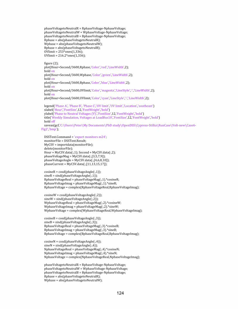
124

phaseVoltagetoNeutralR=RphaseVoltage‐NphaseVoltage;phaseVoltagetoNeutralW=WphaseVoltage‐NphaseVoltage;phaseVoltagetoNeutralB=BphaseVoltage‐NphaseVoltage;Rphase=abs(phaseVoltagetoNeutralR);Wphase=abs(phaseVoltagetoNeutralW);Bphase=abs(phaseVoltagetoNeutralB);OVlimit=253*ones(1,336);UVlimit=216.2*ones(1,336);figure(2);plot(Hour+Second/3600,Rphase,'Color','red','LineWidth',2);holdonplot(Hour+Second/3600,Wphase,'Color','green','LineWidth',2);holdonplot(Hour+Second/3600,Bphase,'Color','blue','LineWidth',2);holdonplot(Hour+Second/3600,OVlimit,'Color','magenta','LineStyle',':','LineWidth',2);holdonplot(Hour+Second/3600,UVlimit,'Color','cyan','LineStyle',':','LineWidth',2);legend('PhaseA','PhaseB','PhaseC','OVlimit','UVlimit','Location','southeast')xlabel('Hour','FontSize',12,'FontWeight','bold')ylabel('PhasetoNeutralVoltages(V)','FontSize',12,'FontWeight','bold')title('WeeklySimulation,VoltagesatLoadBus10','FontSize',12,'FontWeight','bold')holdoffsaveas(gcf,'C:\Users\Peter\MyDocuments\PhDstudy\OpenDSS\Cypress‐Stillia\RunCase\Volt‐new\Case6‐Fig2','bmp');DSSText.Command='exportmonitorsm24';monitorFile=DSSText.Result;MyCSV=importdata(monitorFile);delete(monitorFile);Hour=MyCSV.data(:,1);Second=MyCSV.data(:,2);phaseVoltageMag=MyCSV.data(:,[3,5,7,9]);phaseVoltageAngle=MyCSV.data(:,[4,6,8,10]);phaseCurrent=MyCSV.data(:,[11,13,15,17]);cosineR=cosd(phaseVoltageAngle(:,1));sineR=sind(phaseVoltageAngle(:,1));RphaseVoltageReal=phaseVoltageMag(:,1).*cosineR;RphaseVoltageImag=phaseVoltageMag(:,1).*sineR;RphaseVoltage=complex(RphaseVoltageReal,RphaseVoltageImag);cosineW=cosd(phaseVoltageAngle(:,2));sineW=sind(phaseVoltageAngle(:,2));WphaseVoltageReal=phaseVoltageMag(:,2).*cosineW;WphaseVoltageImag=phaseVoltageMag(:,2).*sineW;WphaseVoltage=complex(WphaseVoltageReal,WphaseVoltageImag);cosineB=cosd(phaseVoltageAngle(:,3));sineB=sind(phaseVoltageAngle(:,3));BphaseVoltageReal=phaseVoltageMag(:,3).*cosineB;BphaseVoltageImag=phaseVoltageMag(:,3).*sineB;BphaseVoltage=complex(BphaseVoltageReal,BphaseVoltageImag);cosineN=cosd(phaseVoltageAngle(:,4));sineN=sind(phaseVoltageAngle(:,4));NphaseVoltageReal=phaseVoltageMag(:,4).*cosineN;NphaseVoltageImag=phaseVoltageMag(:,4).*sineN;NphaseVoltage=complex(NphaseVoltageReal,NphaseVoltageImag);phaseVoltagetoNeutralR=RphaseVoltage‐NphaseVoltage;phaseVoltagetoNeutralW=WphaseVoltage‐NphaseVoltage;phaseVoltagetoNeutralB=BphaseVoltage‐NphaseVoltage;Rphase=abs(phaseVoltagetoNeutralR);Wphase=abs(phaseVoltagetoNeutralW);

125

Bphase=abs(phaseVoltagetoNeutralB);OVlimit=253*ones(1,336);UVlimit=216.2*ones(1,336);figure(3);plot(Hour+Second/3600,Rphase,'Color','red','LineWidth',2);holdonplot(Hour+Second/3600,Wphase,'Color','green','LineWidth',2);holdonplot(Hour+Second/3600,Bphase,'Color','blue','LineWidth',2);holdonplot(Hour+Second/3600,OVlimit,'Color','magenta','LineStyle',':','LineWidth',2);holdonplot(Hour+Second/3600,UVlimit,'Color','cyan','LineStyle',':','LineWidth',2);legend('PhaseA','PhaseB','PhaseC','OVlimit','UVlimit','Location','southeast')xlabel('Hour','FontSize',12,'FontWeight','bold')ylabel('PhasetoNeutralVoltages(V)','FontSize',12,'FontWeight','bold')title('WeeklySimulation,VoltagesatLoadBus11','FontSize',12,'FontWeight','bold')holdoffsaveas(gcf,'C:\Users\Peter\MyDocuments\PhDstudy\OpenDSS\Cypress‐Stillia\RunCase\Volt‐new\Case6‐Fig3','bmp');DSSText.Command='exportmonitorsm25';monitorFile=DSSText.Result;MyCSV=importdata(monitorFile);delete(monitorFile);Hour=MyCSV.data(:,1);Second=MyCSV.data(:,2);phaseVoltageMag=MyCSV.data(:,[3,5,7,9]);phaseVoltageAngle=MyCSV.data(:,[4,6,8,10]);phaseCurrent=MyCSV.data(:,[11,13,15,17]);cosineR=cosd(phaseVoltageAngle(:,1));sineR=sind(phaseVoltageAngle(:,1));RphaseVoltageReal=phaseVoltageMag(:,1).*cosineR;RphaseVoltageImag=phaseVoltageMag(:,1).*sineR;RphaseVoltage=complex(RphaseVoltageReal,RphaseVoltageImag);cosineW=cosd(phaseVoltageAngle(:,2));sineW=sind(phaseVoltageAngle(:,2));WphaseVoltageReal=phaseVoltageMag(:,2).*cosineW;WphaseVoltageImag=phaseVoltageMag(:,2).*sineW;WphaseVoltage=complex(WphaseVoltageReal,WphaseVoltageImag);cosineB=cosd(phaseVoltageAngle(:,3));sineB=sind(phaseVoltageAngle(:,3));BphaseVoltageReal=phaseVoltageMag(:,3).*cosineB;BphaseVoltageImag=phaseVoltageMag(:,3).*sineB;BphaseVoltage=complex(BphaseVoltageReal,BphaseVoltageImag);cosineN=cosd(phaseVoltageAngle(:,4));sineN=sind(phaseVoltageAngle(:,4));NphaseVoltageReal=phaseVoltageMag(:,4).*cosineN;NphaseVoltageImag=phaseVoltageMag(:,4).*sineN;NphaseVoltage=complex(NphaseVoltageReal,NphaseVoltageImag);phaseVoltagetoNeutralR=RphaseVoltage‐NphaseVoltage;phaseVoltagetoNeutralW=WphaseVoltage‐NphaseVoltage;phaseVoltagetoNeutralB=BphaseVoltage‐NphaseVoltage;Rphase=abs(phaseVoltagetoNeutralR);Wphase=abs(phaseVoltagetoNeutralW);Bphase=abs(phaseVoltagetoNeutralB);OVlimit=253*ones(1,336);UVlimit=216.2*ones(1,336);figure(4);

126

plot(Hour+Second/3600,Rphase,'Color','red','LineWidth',2);holdonplot(Hour+Second/3600,Wphase,'Color','green','LineWidth',2);holdonplot(Hour+Second/3600,Bphase,'Color','blue','LineWidth',2);holdonplot(Hour+Second/3600,OVlimit,'Color','magenta','LineStyle',':','LineWidth',2);holdonplot(Hour+Second/3600,UVlimit,'Color','cyan','LineStyle',':','LineWidth',2);legend('PhaseA','PhaseB','PhaseC','OVlimit','UVlimit','Location','southeast')xlabel('Hour','FontSize',12,'FontWeight','bold')ylabel('PhasetoNeutralVoltages(V)','FontSize',12,'FontWeight','bold')title('WeeklySimulation,VoltagesatLoadBus14','FontSize',12,'FontWeight','bold')holdoffsaveas(gcf,'C:\Users\Peter\MyDocuments\PhDstudy\OpenDSS\Cypress‐Stillia\RunCase\Volt‐new\Case6‐Fig4','bmp');DSSText.Command='exportmonitorsm21';monitorFile=DSSText.Result;MyCSV=importdata(monitorFile);delete(monitorFile);Hour=MyCSV.data(:,1);Second=MyCSV.data(:,2);phaseVoltageMag=MyCSV.data(:,[3,5,7,9]);phaseVoltageAngle=MyCSV.data(:,[4,6,8,10]);phaseCurrent=MyCSV.data(:,[11,13,15,17]);cosineR=cosd(phaseVoltageAngle(:,1));sineR=sind(phaseVoltageAngle(:,1));RphaseVoltageReal=phaseVoltageMag(:,1).*cosineR;RphaseVoltageImag=phaseVoltageMag(:,1).*sineR;RphaseVoltage=complex(RphaseVoltageReal,RphaseVoltageImag);cosineW=cosd(phaseVoltageAngle(:,2));sineW=sind(phaseVoltageAngle(:,2));WphaseVoltageReal=phaseVoltageMag(:,2).*cosineW;WphaseVoltageImag=phaseVoltageMag(:,2).*sineW;WphaseVoltage=complex(WphaseVoltageReal,WphaseVoltageImag);cosineB=cosd(phaseVoltageAngle(:,3));sineB=sind(phaseVoltageAngle(:,3));BphaseVoltageReal=phaseVoltageMag(:,3).*cosineB;BphaseVoltageImag=phaseVoltageMag(:,3).*sineB;BphaseVoltage=complex(BphaseVoltageReal,BphaseVoltageImag);cosineN=cosd(phaseVoltageAngle(:,4));sineN=sind(phaseVoltageAngle(:,4));NphaseVoltageReal=phaseVoltageMag(:,4).*cosineN;NphaseVoltageImag=phaseVoltageMag(:,4).*sineN;NphaseVoltage=complex(NphaseVoltageReal,NphaseVoltageImag);phaseVoltagetoNeutralR=RphaseVoltage‐NphaseVoltage;phaseVoltagetoNeutralW=WphaseVoltage‐NphaseVoltage;phaseVoltagetoNeutralB=BphaseVoltage‐NphaseVoltage;Rphase=abs(phaseVoltagetoNeutralR);Wphase=abs(phaseVoltagetoNeutralW);Bphase=abs(phaseVoltagetoNeutralB);OVlimit=253*ones(1,336);UVlimit=216.2*ones(1,336);figure(5);plot(Hour+Second/3600,Rphase,'Color','red','LineWidth',2);holdonplot(Hour+Second/3600,Wphase,'Color','green','LineWidth',2);holdonplot(Hour+Second/3600,Bphase,'Color','blue','LineWidth',2);

127

holdonplot(Hour+Second/3600,OVlimit,'Color','magenta','LineStyle',':','LineWidth',2);holdonplot(Hour+Second/3600,UVlimit,'Color','cyan','LineStyle',':','LineWidth',2);legend('PhaseA','PhaseB','PhaseC','OVlimit','UVlimit','Location','southeast')xlabel('Hour','FontSize',12,'FontWeight','bold')ylabel('PhasetoNeutralVoltages(V)','FontSize',12,'FontWeight','bold')title('WeeklySimulation,VoltagesatLoadBus17','FontSize',12,'FontWeight','bold')holdoffsaveas(gcf,'C:\Users\Peter\MyDocuments\PhDstudy\OpenDSS\Cypress‐Stillia\RunCase\Volt‐new\Case6‐Fig5','bmp');DSSText.Command='exportmonitorsm18';monitorFile=DSSText.Result;MyCSV=importdata(monitorFile);delete(monitorFile);Hour=MyCSV.data(:,1);Second=MyCSV.data(:,2);phaseVoltageMag=MyCSV.data(:,[3,5,7,9]);phaseVoltageAngle=MyCSV.data(:,[4,6,8,10]);phaseCurrent=MyCSV.data(:,[11,13,15,17]);cosineR=cosd(phaseVoltageAngle(:,1));sineR=sind(phaseVoltageAngle(:,1));RphaseVoltageReal=phaseVoltageMag(:,1).*cosineR;RphaseVoltageImag=phaseVoltageMag(:,1).*sineR;RphaseVoltage=complex(RphaseVoltageReal,RphaseVoltageImag);cosineW=cosd(phaseVoltageAngle(:,2));sineW=sind(phaseVoltageAngle(:,2));WphaseVoltageReal=phaseVoltageMag(:,2).*cosineW;WphaseVoltageImag=phaseVoltageMag(:,2).*sineW;WphaseVoltage=complex(WphaseVoltageReal,WphaseVoltageImag);cosineB=cosd(phaseVoltageAngle(:,3));sineB=sind(phaseVoltageAngle(:,3));BphaseVoltageReal=phaseVoltageMag(:,3).*cosineB;BphaseVoltageImag=phaseVoltageMag(:,3).*sineB;BphaseVoltage=complex(BphaseVoltageReal,BphaseVoltageImag);cosineN=cosd(phaseVoltageAngle(:,4));sineN=sind(phaseVoltageAngle(:,4));NphaseVoltageReal=phaseVoltageMag(:,4).*cosineN;NphaseVoltageImag=phaseVoltageMag(:,4).*sineN;NphaseVoltage=complex(NphaseVoltageReal,NphaseVoltageImag);phaseVoltagetoNeutralR=RphaseVoltage‐NphaseVoltage;phaseVoltagetoNeutralW=WphaseVoltage‐NphaseVoltage;phaseVoltagetoNeutralB=BphaseVoltage‐NphaseVoltage;Rphase=abs(phaseVoltagetoNeutralR);Wphase=abs(phaseVoltagetoNeutralW);Bphase=abs(phaseVoltagetoNeutralB);OVlimit=253*ones(1,336);UVlimit=216.2*ones(1,336);figure(6);plot(Hour+Second/3600,Rphase,'Color','red','LineWidth',2);holdonplot(Hour+Second/3600,Wphase,'Color','green','LineWidth',2);holdonplot(Hour+Second/3600,Bphase,'Color','blue','LineWidth',2);holdonplot(Hour+Second/3600,OVlimit,'Color','magenta','LineStyle',':','LineWidth',2);holdonplot(Hour+Second/3600,UVlimit,'Color','cyan','LineStyle',':','LineWidth',2);

128

legend('PhaseA','PhaseB','PhaseC','OVlimit','UVlimit','Location','southeast')xlabel('Hour','FontSize',12,'FontWeight','bold')ylabel('PhasetoNeutralVoltages(V)','FontSize',12,'FontWeight','bold')title('WeeklySimulation,VoltagesatLoadBus20','FontSize',12,'FontWeight','bold')holdoffsaveas(gcf,'C:\Users\Peter\MyDocuments\PhDstudy\OpenDSS\Cypress‐Stillia\RunCase\Volt‐new\Case6‐Fig6','bmp');

MATLAB Codes for Voltage Unbalance Analysis %MatLabcodeforvoltageunbalanceanalysis%TorunthisMatLabcode,makesurethecurrentfolderpointstothe%locationwhereallthefilesrequiredbytheDSSprogramarelocatedclearall;DSSObj=actxserver('OpenDSSEngine.dss');Start=DSSObj.Start(0);[DSSStartOK,DSSObj,DSSText]=DSSStartup;%SetuptheinterfacevariablesDSSCircuit=DSSObj.ActiveCircuit;DSSSolution=DSSCircuit.Solution;DSSText.Command='Compile(C:\ProgramFiles\OpenDSS\Examples\Jemena\SHM14_Cypress‐Stillia_V23b.dss)';%AddanEnergyMeterobjectsothedistancesdownthefeederarecomputedDSSText.Command='NewEnergyMeter.E1Line.LINE11';%AddaMonitor,tooDSSText.Command='NewMonitor.FeederEndLine.LINE11';%NewLineDropCompensationsettingdefaultisVreg=63.5R=1.16X=1.97DSSText.Command='RegControl.Reg1.Vreg=65.3R=0X=0';%ChangetheloadtypeatSHM22kVbusDSSText.Command='NewLoad.LOAD1Bus1=LoadBus2kV=22kVA=18000PF=0.9duty=Bus_weekly';%ConnectPV1andPV2toselectedphasesDSSText.Command='PVSystem.PV1.Bus1=LoadBus12.3.4';DSSText.Command='PVSystem.PV2.Bus1=LoadBus21.3.4';%‐‐‐‐‐‐‐‐‐‐‐‐‐‐‐‐‐‐‐‐‐‐‐‐‐‐‐‐‐‐‐‐‐‐‐‐‐‐‐‐‐‐‐‐‐‐‐‐‐‐‐‐‐‐‐‐‐‐‐‐‐‐‐‐‐‐‐‐‐%Runaweeklyanalysisandplotthevoltagesandcurrentsmeasuredbythemonitors%The3‐phasevoltagesaremeasuredbetweenthephasesandneutral%‐‐‐‐‐‐‐‐‐‐‐‐‐‐‐‐‐‐‐‐‐‐‐‐‐‐‐‐‐‐‐‐‐‐‐‐‐‐‐‐‐‐‐‐‐‐‐‐‐‐‐‐‐‐‐‐‐‐‐‐‐‐‐‐‐‐‐‐DSSText.command='setmode=duty';DSSCircuit.Solution.Number=1;DSSCircuit.Solution.Stepsize=1800;DSSCircuit.Solution.Hour=0;fori=1:336DSSCircuit.Solution.Solve;endDSSText.Command='exportmonitorsm6';monitorFile=DSSText.Result;MyCSV=importdata(monitorFile);delete(monitorFile);

129

Hour=MyCSV.data(:,1);Second=MyCSV.data(:,2);phaseVoltageMag=MyCSV.data(:,[3,5,7,9]);phaseVoltageAngle=MyCSV.data(:,[4,6,8,10]);cosineR=cosd(phaseVoltageAngle(:,1));sineR=sind(phaseVoltageAngle(:,1));RphaseVoltageReal=phaseVoltageMag(:,1).*cosineR;RphaseVoltageImag=phaseVoltageMag(:,1).*sineR;RphaseVoltage=complex(RphaseVoltageReal,RphaseVoltageImag);cosineW=cosd(phaseVoltageAngle(:,2));sineW=sind(phaseVoltageAngle(:,2));WphaseVoltageReal=phaseVoltageMag(:,2).*cosineW;WphaseVoltageImag=phaseVoltageMag(:,2).*sineW;WphaseVoltage=complex(WphaseVoltageReal,WphaseVoltageImag);cosineB=cosd(phaseVoltageAngle(:,3));sineB=sind(phaseVoltageAngle(:,3));BphaseVoltageReal=phaseVoltageMag(:,3).*cosineB;BphaseVoltageImag=phaseVoltageMag(:,3).*sineB;BphaseVoltage=complex(BphaseVoltageReal,BphaseVoltageImag);cosineN=cosd(phaseVoltageAngle(:,4));sineN=sind(phaseVoltageAngle(:,4));NphaseVoltageReal=phaseVoltageMag(:,4).*cosineN;NphaseVoltageImag=phaseVoltageMag(:,4).*sineN;NphaseVoltage=complex(NphaseVoltageReal,NphaseVoltageImag);phaseVoltagetoNeutralR=RphaseVoltage‐NphaseVoltage;phaseVoltagetoNeutralW=WphaseVoltage‐NphaseVoltage;phaseVoltagetoNeutralB=BphaseVoltage‐NphaseVoltage;Rphase=abs(phaseVoltagetoNeutralR);%phase‐to‐neutralvoltagemagnitudeWphase=abs(phaseVoltagetoNeutralW);Bphase=abs(phaseVoltagetoNeutralB);RphaseAngle=angle(phaseVoltagetoNeutralR);%inradiansWphaseAngle=angle(phaseVoltagetoNeutralW);BphaseAngle=angle(phaseVoltagetoNeutralB);RWphaseAngle=RphaseAngle‐WphaseAngle;%inradiansWBphaseAngle=WphaseAngle‐BphaseAngle;BRphaseAngle=BphaseAngle‐RphaseAngle;VoltageUnbalance_Num=sqrt((Rphase.^2+Wphase.^2+Bphase.^2)*2+Rphase.*Wphase.*cos(RWphaseAngle+1.0472)*2+Wphase.*Bphase.*cos(WBphaseAngle+1.0472)*2+Bphase.*Rphase.*cos(BRphaseAngle+1.0472)*2);VoltageUnbalance_Dem=sqrt((Rphase.^2+Wphase.^2+Bphase.^2)+Rphase.*Wphase.*cos(RWphaseAngle‐2.0944)*2+Wphase.*Bphase.*cos(WBphaseAngle‐2.0944)*2+Bphase.*Rphase.*cos(BRphaseAngle‐2.0944)*2);VoltageUnbalance_bus9=100*(VoltageUnbalance_Num./VoltageUnbalance_Dem);%voltagebalancein%xlswrite('C:\Users\Peter\MyDocuments\PhDstudy\OpenDSS\Cypress‐Stillia\RunCase\Unbalance‐new\Phaseallocation\Monitors‐phaseallocation.xlsx',VoltageUnbalance_bus9,'Case9','A2:A337');clear('phaseVoltageMag','phaseVoltageAngle');DSSText.Command='exportmonitorsm23';monitorFile=DSSText.Result;MyCSV=importdata(monitorFile);delete(monitorFile);Hour=MyCSV.data(:,1);Second=MyCSV.data(:,2);phaseVoltageMag=MyCSV.data(:,[3,5,7,9]);phaseVoltageAngle=MyCSV.data(:,[4,6,8,10]);cosineR=cosd(phaseVoltageAngle(:,1));sineR=sind(phaseVoltageAngle(:,1));RphaseVoltageReal=phaseVoltageMag(:,1).*cosineR;

130

RphaseVoltageImag=phaseVoltageMag(:,1).*sineR;RphaseVoltage=complex(RphaseVoltageReal,RphaseVoltageImag);cosineW=cosd(phaseVoltageAngle(:,2));sineW=sind(phaseVoltageAngle(:,2));WphaseVoltageReal=phaseVoltageMag(:,2).*cosineW;WphaseVoltageImag=phaseVoltageMag(:,2).*sineW;WphaseVoltage=complex(WphaseVoltageReal,WphaseVoltageImag);cosineB=cosd(phaseVoltageAngle(:,3));sineB=sind(phaseVoltageAngle(:,3));BphaseVoltageReal=phaseVoltageMag(:,3).*cosineB;BphaseVoltageImag=phaseVoltageMag(:,3).*sineB;BphaseVoltage=complex(BphaseVoltageReal,BphaseVoltageImag);cosineN=cosd(phaseVoltageAngle(:,4));sineN=sind(phaseVoltageAngle(:,4));NphaseVoltageReal=phaseVoltageMag(:,4).*cosineN;NphaseVoltageImag=phaseVoltageMag(:,4).*sineN;NphaseVoltage=complex(NphaseVoltageReal,NphaseVoltageImag);phaseVoltagetoNeutralR=RphaseVoltage‐NphaseVoltage;phaseVoltagetoNeutralW=WphaseVoltage‐NphaseVoltage;phaseVoltagetoNeutralB=BphaseVoltage‐NphaseVoltage;Rphase=abs(phaseVoltagetoNeutralR);%phase‐to‐neutralvoltagemagnitudeWphase=abs(phaseVoltagetoNeutralW);Bphase=abs(phaseVoltagetoNeutralB);RphaseAngle=angle(phaseVoltagetoNeutralR);%inradiansWphaseAngle=angle(phaseVoltagetoNeutralW);BphaseAngle=angle(phaseVoltagetoNeutralB);RWphaseAngle=RphaseAngle‐WphaseAngle;%inradiansWBphaseAngle=WphaseAngle‐BphaseAngle;BRphaseAngle=BphaseAngle‐RphaseAngle;VoltageUnbalance_Num=sqrt((Rphase.^2+Wphase.^2+Bphase.^2)*2+Rphase.*Wphase.*cos(RWphaseAngle+1.0472)*2+Wphase.*Bphase.*cos(WBphaseAngle+1.0472)*2+Bphase.*Rphase.*cos(BRphaseAngle+1.0472)*2);VoltageUnbalance_Dem=sqrt((Rphase.^2+Wphase.^2+Bphase.^2)+Rphase.*Wphase.*cos(RWphaseAngle‐2.0944)*2+Wphase.*Bphase.*cos(WBphaseAngle‐2.0944)*2+Bphase.*Rphase.*cos(BRphaseAngle‐2.0944)*2);VoltageUnbalance_bus10=100*(VoltageUnbalance_Num./VoltageUnbalance_Dem);%voltagebalancein%xlswrite('C:\Users\Peter\MyDocuments\PhDstudy\OpenDSS\Cypress‐Stillia\RunCase\Unbalance‐new\Phaseallocation\Monitors‐phaseallocation.xlsx',VoltageUnbalance_bus10,'Case9','B2:B337');clear('phaseVoltageMag','phaseVoltageAngle');DSSText.Command='exportmonitorsm24';monitorFile=DSSText.Result;MyCSV=importdata(monitorFile);delete(monitorFile);Hour=MyCSV.data(:,1);Second=MyCSV.data(:,2);phaseVoltageMag=MyCSV.data(:,[3,5,7,9]);phaseVoltageAngle=MyCSV.data(:,[4,6,8,10]);cosineR=cosd(phaseVoltageAngle(:,1));sineR=sind(phaseVoltageAngle(:,1));RphaseVoltageReal=phaseVoltageMag(:,1).*cosineR;RphaseVoltageImag=phaseVoltageMag(:,1).*sineR;RphaseVoltage=complex(RphaseVoltageReal,RphaseVoltageImag);cosineW=cosd(phaseVoltageAngle(:,2));sineW=sind(phaseVoltageAngle(:,2));WphaseVoltageReal=phaseVoltageMag(:,2).*cosineW;WphaseVoltageImag=phaseVoltageMag(:,2).*sineW;

131

WphaseVoltage=complex(WphaseVoltageReal,WphaseVoltageImag);cosineB=cosd(phaseVoltageAngle(:,3));sineB=sind(phaseVoltageAngle(:,3));BphaseVoltageReal=phaseVoltageMag(:,3).*cosineB;BphaseVoltageImag=phaseVoltageMag(:,3).*sineB;BphaseVoltage=complex(BphaseVoltageReal,BphaseVoltageImag);cosineN=cosd(phaseVoltageAngle(:,4));sineN=sind(phaseVoltageAngle(:,4));NphaseVoltageReal=phaseVoltageMag(:,4).*cosineN;NphaseVoltageImag=phaseVoltageMag(:,4).*sineN;NphaseVoltage=complex(NphaseVoltageReal,NphaseVoltageImag);phaseVoltagetoNeutralR=RphaseVoltage‐NphaseVoltage;phaseVoltagetoNeutralW=WphaseVoltage‐NphaseVoltage;phaseVoltagetoNeutralB=BphaseVoltage‐NphaseVoltage;Rphase=abs(phaseVoltagetoNeutralR);%phase‐to‐neutralvoltagemagnitudeWphase=abs(phaseVoltagetoNeutralW);Bphase=abs(phaseVoltagetoNeutralB);RphaseAngle=angle(phaseVoltagetoNeutralR);%inradiansWphaseAngle=angle(phaseVoltagetoNeutralW);BphaseAngle=angle(phaseVoltagetoNeutralB);RWphaseAngle=RphaseAngle‐WphaseAngle;%inradiansWBphaseAngle=WphaseAngle‐BphaseAngle;BRphaseAngle=BphaseAngle‐RphaseAngle;VoltageUnbalance_Num=sqrt((Rphase.^2+Wphase.^2+Bphase.^2)*2+Rphase.*Wphase.*cos(RWphaseAngle+1.0472)*2+Wphase.*Bphase.*cos(WBphaseAngle+1.0472)*2+Bphase.*Rphase.*cos(BRphaseAngle+1.0472)*2);VoltageUnbalance_Dem=sqrt((Rphase.^2+Wphase.^2+Bphase.^2)+Rphase.*Wphase.*cos(RWphaseAngle‐2.0944)*2+Wphase.*Bphase.*cos(WBphaseAngle‐2.0944)*2+Bphase.*Rphase.*cos(BRphaseAngle‐2.0944)*2);VoltageUnbalance_bus11=100*(VoltageUnbalance_Num./VoltageUnbalance_Dem);%voltagebalancein%xlswrite('C:\Users\Peter\MyDocuments\PhDstudy\OpenDSS\Cypress‐Stillia\RunCase\Unbalance‐new\Phaseallocation\Monitors‐phaseallocation.xlsx',VoltageUnbalance_bus11,'Case9','C2:C337');clear('phaseVoltageMag','phaseVoltageAngle');DSSText.Command='exportmonitorsm18';monitorFile=DSSText.Result;MyCSV=importdata(monitorFile);delete(monitorFile);Hour=MyCSV.data(:,1);Second=MyCSV.data(:,2);phaseVoltageMag=MyCSV.data(:,[3,5,7,9]);phaseVoltageAngle=MyCSV.data(:,[4,6,8,10]);cosineR=cosd(phaseVoltageAngle(:,1));sineR=sind(phaseVoltageAngle(:,1));RphaseVoltageReal=phaseVoltageMag(:,1).*cosineR;RphaseVoltageImag=phaseVoltageMag(:,1).*sineR;RphaseVoltage=complex(RphaseVoltageReal,RphaseVoltageImag);cosineW=cosd(phaseVoltageAngle(:,2));sineW=sind(phaseVoltageAngle(:,2));WphaseVoltageReal=phaseVoltageMag(:,2).*cosineW;WphaseVoltageImag=phaseVoltageMag(:,2).*sineW;WphaseVoltage=complex(WphaseVoltageReal,WphaseVoltageImag);cosineB=cosd(phaseVoltageAngle(:,3));sineB=sind(phaseVoltageAngle(:,3));BphaseVoltageReal=phaseVoltageMag(:,3).*cosineB;BphaseVoltageImag=phaseVoltageMag(:,3).*sineB;

132

BphaseVoltage=complex(BphaseVoltageReal,BphaseVoltageImag);cosineN=cosd(phaseVoltageAngle(:,4));sineN=sind(phaseVoltageAngle(:,4));NphaseVoltageReal=phaseVoltageMag(:,4).*cosineN;NphaseVoltageImag=phaseVoltageMag(:,4).*sineN;NphaseVoltage=complex(NphaseVoltageReal,NphaseVoltageImag);phaseVoltagetoNeutralR=RphaseVoltage‐NphaseVoltage;phaseVoltagetoNeutralW=WphaseVoltage‐NphaseVoltage;phaseVoltagetoNeutralB=BphaseVoltage‐NphaseVoltage;Rphase=abs(phaseVoltagetoNeutralR);%phase‐to‐neutralvoltagemagnitudeWphase=abs(phaseVoltagetoNeutralW);Bphase=abs(phaseVoltagetoNeutralB);RphaseAngle=angle(phaseVoltagetoNeutralR);%inradiansWphaseAngle=angle(phaseVoltagetoNeutralW);BphaseAngle=angle(phaseVoltagetoNeutralB);RWphaseAngle=RphaseAngle‐WphaseAngle;%inradiansWBphaseAngle=WphaseAngle‐BphaseAngle;BRphaseAngle=BphaseAngle‐RphaseAngle;VoltageUnbalance_Num=sqrt((Rphase.^2+Wphase.^2+Bphase.^2)*2+Rphase.*Wphase.*cos(RWphaseAngle+1.0472)*2+Wphase.*Bphase.*cos(WBphaseAngle+1.0472)*2+Bphase.*Rphase.*cos(BRphaseAngle+1.0472)*2);VoltageUnbalance_Dem=sqrt((Rphase.^2+Wphase.^2+Bphase.^2)+Rphase.*Wphase.*cos(RWphaseAngle‐2.0944)*2+Wphase.*Bphase.*cos(WBphaseAngle‐2.0944)*2+Bphase.*Rphase.*cos(BRphaseAngle‐2.0944)*2);VoltageUnbalance_bus20=100*(VoltageUnbalance_Num./VoltageUnbalance_Dem);%voltagebalancein%xlswrite('C:\Users\Peter\MyDocuments\PhDstudy\OpenDSS\Cypress‐Stillia\RunCase\Unbalance‐new\Phaseallocation\Monitors‐phaseallocation.xlsx',VoltageUnbalance_bus20,'Case9','F2:F337');clear('phaseVoltageMag','phaseVoltageAngle');DSSText.Command='exportmonitorsm25';monitorFile=DSSText.Result;MyCSV=importdata(monitorFile);delete(monitorFile);Hour=MyCSV.data(:,1);Second=MyCSV.data(:,2);phaseVoltageMag=MyCSV.data(:,[3,5,7,9]);phaseVoltageAngle=MyCSV.data(:,[4,6,8,10]);cosineR=cosd(phaseVoltageAngle(:,1));sineR=sind(phaseVoltageAngle(:,1));RphaseVoltageReal=phaseVoltageMag(:,1).*cosineR;RphaseVoltageImag=phaseVoltageMag(:,1).*sineR;RphaseVoltage=complex(RphaseVoltageReal,RphaseVoltageImag);cosineW=cosd(phaseVoltageAngle(:,2));sineW=sind(phaseVoltageAngle(:,2));WphaseVoltageReal=phaseVoltageMag(:,2).*cosineW;WphaseVoltageImag=phaseVoltageMag(:,2).*sineW;WphaseVoltage=complex(WphaseVoltageReal,WphaseVoltageImag);cosineB=cosd(phaseVoltageAngle(:,3));sineB=sind(phaseVoltageAngle(:,3));BphaseVoltageReal=phaseVoltageMag(:,3).*cosineB;BphaseVoltageImag=phaseVoltageMag(:,3).*sineB;BphaseVoltage=complex(BphaseVoltageReal,BphaseVoltageImag);cosineN=cosd(phaseVoltageAngle(:,4));sineN=sind(phaseVoltageAngle(:,4));NphaseVoltageReal=phaseVoltageMag(:,4).*cosineN;NphaseVoltageImag=phaseVoltageMag(:,4).*sineN;NphaseVoltage=complex(NphaseVoltageReal,NphaseVoltageImag);

133

phaseVoltagetoNeutralR=RphaseVoltage‐NphaseVoltage;phaseVoltagetoNeutralW=WphaseVoltage‐NphaseVoltage;phaseVoltagetoNeutralB=BphaseVoltage‐NphaseVoltage;Rphase=abs(phaseVoltagetoNeutralR);%phase‐to‐neutralvoltagemagnitudeWphase=abs(phaseVoltagetoNeutralW);Bphase=abs(phaseVoltagetoNeutralB);RphaseAngle=angle(phaseVoltagetoNeutralR);%inradiansWphaseAngle=angle(phaseVoltagetoNeutralW);BphaseAngle=angle(phaseVoltagetoNeutralB);RWphaseAngle=RphaseAngle‐WphaseAngle;%inradiansWBphaseAngle=WphaseAngle‐BphaseAngle;BRphaseAngle=BphaseAngle‐RphaseAngle;VoltageUnbalance_Num=sqrt((Rphase.^2+Wphase.^2+Bphase.^2)*2+Rphase.*Wphase.*cos(RWphaseAngle+1.0472)*2+Wphase.*Bphase.*cos(WBphaseAngle+1.0472)*2+Bphase.*Rphase.*cos(BRphaseAngle+1.0472)*2);VoltageUnbalance_Dem=sqrt((Rphase.^2+Wphase.^2+Bphase.^2)+Rphase.*Wphase.*cos(RWphaseAngle‐2.0944)*2+Wphase.*Bphase.*cos(WBphaseAngle‐2.0944)*2+Bphase.*Rphase.*cos(BRphaseAngle‐2.0944)*2);VoltageUnbalance_bus14=100*(VoltageUnbalance_Num./VoltageUnbalance_Dem);%voltagebalancein%xlswrite('C:\Users\Peter\MyDocuments\PhDstudy\OpenDSS\Cypress‐Stillia\RunCase\Unbalance‐new\Phaseallocation\Monitors‐phaseallocation.xlsx',VoltageUnbalance_bus14,'Case9','d2:d337');clear('phaseVoltageMag','phaseVoltageAngle');DSSText.Command='exportmonitorsm21';monitorFile=DSSText.Result;MyCSV=importdata(monitorFile);delete(monitorFile);Hour=MyCSV.data(:,1);Second=MyCSV.data(:,2);phaseVoltageMag=MyCSV.data(:,[3,5,7,9]);phaseVoltageAngle=MyCSV.data(:,[4,6,8,10]);cosineR=cosd(phaseVoltageAngle(:,1));sineR=sind(phaseVoltageAngle(:,1));RphaseVoltageReal=phaseVoltageMag(:,1).*cosineR;RphaseVoltageImag=phaseVoltageMag(:,1).*sineR;RphaseVoltage=complex(RphaseVoltageReal,RphaseVoltageImag);cosineW=cosd(phaseVoltageAngle(:,2));sineW=sind(phaseVoltageAngle(:,2));WphaseVoltageReal=phaseVoltageMag(:,2).*cosineW;WphaseVoltageImag=phaseVoltageMag(:,2).*sineW;WphaseVoltage=complex(WphaseVoltageReal,WphaseVoltageImag);cosineB=cosd(phaseVoltageAngle(:,3));sineB=sind(phaseVoltageAngle(:,3));BphaseVoltageReal=phaseVoltageMag(:,3).*cosineB;BphaseVoltageImag=phaseVoltageMag(:,3).*sineB;BphaseVoltage=complex(BphaseVoltageReal,BphaseVoltageImag);cosineN=cosd(phaseVoltageAngle(:,4));sineN=sind(phaseVoltageAngle(:,4));NphaseVoltageReal=phaseVoltageMag(:,4).*cosineN;NphaseVoltageImag=phaseVoltageMag(:,4).*sineN;NphaseVoltage=complex(NphaseVoltageReal,NphaseVoltageImag);phaseVoltagetoNeutralR=RphaseVoltage‐NphaseVoltage;phaseVoltagetoNeutralW=WphaseVoltage‐NphaseVoltage;phaseVoltagetoNeutralB=BphaseVoltage‐NphaseVoltage;Rphase=abs(phaseVoltagetoNeutralR);%phase‐to‐neutralvoltagemagnitudeWphase=abs(phaseVoltagetoNeutralW);Bphase=abs(phaseVoltagetoNeutralB);

134

RphaseAngle=angle(phaseVoltagetoNeutralR);%inradiansWphaseAngle=angle(phaseVoltagetoNeutralW);BphaseAngle=angle(phaseVoltagetoNeutralB);RWphaseAngle=RphaseAngle‐WphaseAngle;%inradiansWBphaseAngle=WphaseAngle‐BphaseAngle;BRphaseAngle=BphaseAngle‐RphaseAngle;VoltageUnbalance_Num=sqrt((Rphase.^2+Wphase.^2+Bphase.^2)*2+Rphase.*Wphase.*cos(RWphaseAngle+1.0472)*2+Wphase.*Bphase.*cos(WBphaseAngle+1.0472)*2+Bphase.*Rphase.*cos(BRphaseAngle+1.0472)*2);VoltageUnbalance_Dem=sqrt((Rphase.^2+Wphase.^2+Bphase.^2)+Rphase.*Wphase.*cos(RWphaseAngle‐2.0944)*2+Wphase.*Bphase.*cos(WBphaseAngle‐2.0944)*2+Bphase.*Rphase.*cos(BRphaseAngle‐2.0944)*2);VoltageUnbalance_bus17=100*(VoltageUnbalance_Num./VoltageUnbalance_Dem);%voltagebalancein%xlswrite('C:\Users\Peter\MyDocuments\PhDstudy\OpenDSS\Cypress‐Stillia\RunCase\Unbalance‐new\Phaseallocation\Monitors‐phaseallocation.xlsx',VoltageUnbalance_bus17,'Case9','e2:e337');clear('phaseVoltageMag','phaseVoltageAngle');figure(9);plot(Hour+Second/3600,VoltageUnbalance_bus9,'Color','green','LineWidth',1);holdonplot(Hour+Second/3600,VoltageUnbalance_bus10,'Color','cyan','LineWidth',1);holdonplot(Hour+Second/3600,VoltageUnbalance_bus11,'Color','magenta','LineWidth',1);holdonplot(Hour+Second/3600,VoltageUnbalance_bus20,'Color','blue','LineWidth',1);holdonplot(Hour+Second/3600,VoltageUnbalance_bus14,'Color','red','LineWidth',1);holdonplot(Hour+Second/3600,VoltageUnbalance_bus17,'Color','black','LineWidth',1);legend('LoadBus9','LoadBus10','LoadBus11','LoadBus20','LoadBus14','LoadBus17','Location','best')xlabel('Hour','FontSize',12,'FontWeight','bold')ylabel('VoltageUnbalancein%','FontSize',12,'FontWeight','bold')ylim([01.4])title('UnbalanceVoltagesatLoadBuses','FontSize',12,'FontWeight','bold')holdoffsaveas(gcf,'C:\Users\Peter\MyDocuments\PhDstudy\OpenDSS\Cypress‐Stillia\RunCase\Unbalance‐New\Phaseallocation\Scenario6Case9‐allloadbuses','bmp');

135

References

1. Ochoa, L.F. and P. Mancarella. Low-carbon LV networks: Challenges for planning and operation. in Power and Energy Society General Meeting, 2012 IEEE. 2012. IEEE.

2. Elphick, S., et al. The Australian Long Term Power Quality Survey project update. in Proceedings of 14th International Conference on Harmonics and Quality of Power - ICHQP 2010. 2010.

3. Navarro, A., et al. Impacts of photovoltaics on low voltage networks: A case study for the North West of England. in 22nd International Conference and Exhibition on Electricity Distribution (CIRED 2013). 2013.

4. Inc, R.W.B., Distributed Renewable Energy Operating Impacts and Valuation Study. 2009, Arizona Public Service.

5. Shafiullah, G.M., et al., Prospects of renewable energy – a feasibility study in the Australian context. Renewable Energy, 2012. 39(1): p. 183-197.

6. McConnell, D., et al., Retrospective modeling of the merit-order effect on wholesale electricity prices from distributed photovoltaic generation in the Australian National Electricity Market. Energy Policy, 2013. 58: p. 17-27.

7. Marinopoulos, A.G., M.C. Alexiadis, and P.S. Dokopoulos, Energy losses in a distribution line with distributed generation based on stochastic power flow. Electric Power Systems Research, 2011. 81(10): p. 1986-1994.

8. Medina, A., J.C. Hernandez, and F. Jurado. Optimal Placement and Sizing Procedure for PV Systems on Radial Distribution Systems. in 2006 International Conference on Power System Technology. 2006.

9. Marinopoulos, A.G., M.C. Alexiadis, and P.S. Dokopoulos, A Correlation Index to Evaluate Impact of PV Installation on Joule Losses. IEEE Transactions on Power Systems, 2011. 26(3): p. 1564-1572.

10. Barbeiro, P.N.P., et al. Evaluation of the impact of large scale integration of micro-generation units in low and Medium Voltage distribution networks. in 2010 IEEE Conference on Innovative Technologies for an Efficient and Reliable Electricity Supply. 2010.

11. Ropp, M., et al. Review of potential problems and utility concerns arising from high penetration levels of photovoltaics in distribution systems. in 2008 33rd IEEE Photovoltaic Specialists Conference. 2008.

12. Gonzalez, C., et al. LV distribution network feeders in Belgium and power quality issues due to increasing PV penetration levels. in 2012 3rd IEEE PES Innovative Smart Grid Technologies Europe (ISGT Europe). 2012.

13. Eltawil, M.A. and Z. Zhao, Grid-connected photovoltaic power systems: Technical and potential problems—A review. Renewable and Sustainable Energy Reviews, 2010. 14(1): p. 112-129.

14. Braun, M., et al., Is the distribution grid ready to accept large-scale photovoltaic deployment? State of the art, progress, and future prospects. Progress in Photovoltaics: Research and Applications, 2012. 20(6): p. 681-697.

15. Purvins, A. and B. Klebow, Technical grid connection guides for distributed electricity generation systems: a new DERlab database has come alive. IET Renewable Power Generation, 2015. 9(8): p. 1087-1092.

16. Kimmo Lummi, P.T., Antti Rautiainen, Pertti Järventausta. Implementation possibilities of power-based distribution tariff by using smart metering technology. in CIRED. 2015. Lyon, France.

17. Electricity distribution investment - what regulatory framework do we need. 2014, Eurelectric.

18. Ramos, S. and Z. Vale. Data Mining techniques to support the classification of MV electricity customers. in 2008 IEEE Power and Energy Society General Meeting - Conversion and Delivery of Electrical Energy in the 21st Century. 2008.

19. Haben, S., C. Singleton, and P. Grindrod, Analysis and Clustering of Residential Customers Energy Behavioral Demand Using Smart Meter Data. IEEE Transactions on Smart Grid, 2016. 7(1): p. 136-144.

20. Pan, E., D. Wang, and Z. Han, Analyzing Big Smart Metering Data Towards Differentiated User Services: A Sublinear Approach. IEEE Transactions on Big Data, 2016. 2(3): p. 249-261.

136

21. Valigi, E. and E.d. Marino. Networks optimization with advanced meter infrastructure and smart meters. in CIRED 2009 - 20th International Conference and Exhibition on Electricity Distribution - Part 1. 2009.

22. Han, S., et al., An Automated Impedance Estimation Method in Low-Voltage Distribution Network for Coordinated Voltage Regulation. IEEE Transactions on Smart Grid, 2015: p. 1-9.

23. Pezeshki, H. and P.J. Wolfs. Consumer phase identification in a three phase unbalanced LV distribution network. in 2012 3rd IEEE PES Innovative Smart Grid Technologies Europe (ISGT Europe). 2012.

24. Satya Jayadev P, A.R., Nirav P Bhatt, Ramkrishna Pasumarthy, A Novel Approach for Phase Identification in Smart Grids Using Graph Theory and Principal Component Analysis.pdf, in 2016 American Control Conference. 2016: Boston Marriott Copley Place. Boston, MA, USA.

25. Shahnia, F., P.J. Wolfs, and A. Ghosh, Voltage Unbalance Reduction in Low Voltage Feeders by Dynamic Switching of Residential Customers Among Three Phases. IEEE Transactions on Smart Grid, 2014. 5(3): p. 1318-1327.

26. Lim, Y.S. and J.H. Tang, Experimental study on flicker emissions by photovoltaic systems on highly cloudy region: A case study in Malaysia. Renewable Energy, 2014. 64: p. 61-70.

27. Cameron, C.P., W.E. Boyson, and D.M. Riley. Comparison of PV system performance-model predictions with measured PV system performance. in 2008 33rd IEEE Photovoltaic Specialists Conference. 2008.

28. Chatterjee, A., A. Keyhani, and D. Kapoor, Identification of Photovoltaic Source Models. IEEE Transactions on Energy Conversion, 2011. 26(3): p. 883-889.

29. Bo, Z., et al. Research on model for photovoltaic system power forecasting. in CICED 2010 Proceedings. 2010.

30. Ciric, R.M., A.P. Feltrin, and L.F. Ochoa, Power flow in four-wire distribution networks-general approach. IEEE Transactions on Power Systems, 2003. 18(4): p. 1283-1290.

31. Sunderland, K.M. and M.F. Conlon. 4-Wire load flow analysis of a representative urban network incoprating SSEG. in 2012 47th International Universities Power Engineering Conference (UPEC). 2012.

32. Urquhart, A.J. and M. Thomson, Series impedance of distribution cables with sector-shaped conductors. IET Generation, Transmission & Distribution, 2015. 9(16): p. 2679-2685.

33. Kersting, W.H. and R.K. Green. The application of Carson's equation to the steady-state analysis of distribution feeders. in 2011 IEEE/PES Power Systems Conference and Exposition. 2011.

34. Shahnia, F., et al., Voltage imbalance analysis in residential low voltage distribution networks with rooftop PVs. Electric Power Systems Research, 2011. 81(9): p. 1805-1814.

35. Alam, M.J.E., K.M. Muttaqi, and D. Sutanto, A SAX-Based Advanced Computational Tool for Assessment of Clustered Rooftop Solar PV Impacts on LV and MV Networks in Smart Grid. IEEE Transactions on Smart Grid, 2013. 4(1): p. 577-585.

36. Navarro, A., L.F. Ochoa, and D. Randles. Monte Carlo-based assessment of PV impacts on real UK low voltage networks. in 2013 IEEE Power & Energy Society General Meeting. 2013.

37. Ruiz-Rodriguez, F.J., J.C. Hernández, and F. Jurado, Probabilistic load flow for photovoltaic distributed generation using the Cornish–Fisher expansion. Electric Power Systems Research, 2012. 89: p. 129-138.

38. Rigoni, V., et al., Representative Residential LV Feeders: A Case Study for the North West of England. IEEE Transactions on Power Systems, 2016. 31(1): p. 348-360.

39. Fila, M., et al. Flexible voltage control to support Distributed Generation in distribution networks. in 2008 43rd International Universities Power Engineering Conference. 2008.

40. Vincent Thornley, N.J., Peter Reay, Jonathan Hill, Christine Barbier. Field experience with active network management of distribution networks with distributed generation. in CIRED. 2007. Vienna, Austria.

41. Alnaser, S.W. and L.F. Ochoa, Advanced Network Management Systems: A Risk-Based AC OPF Approach. IEEE Transactions on Power Systems, 2015. 30(1): p. 409-418.

42. Harrison, G.P., et al., Hybrid GA and OPF evaluation of network capacity for distributed generation connections. Electric Power Systems Research, 2008. 78(3): p. 392-398.

137

43. Hengsritawat, V., T. Tayjasanant, and N. Nimpitiwan, Optimal sizing of photovoltaic distributed generators in a distribution system with consideration of solar radiation and harmonic distortion. International Journal of Electrical Power & Energy Systems, 2012. 39(1): p. 36-47.

44. Ballanti, A., et al. Assessing the benefits of PV var absorption on the hosting capacity of LV feeders. in IEEE PES ISGT Europe 2013. 2013.

45. T. Stetz, W.Y., M. Braun. Voltage Control in Distribution Systems with High Level PV Penetration- Improving Absorption Capacity for PV Systems by Reactive Power Supply. in 25th European Photovoltaic Solar Energy Conference and Exhibition / 5th World Conference on Photovoltaic Energy Conversion. 2010. Valencia, Spain.

46. Herman, L., B. Blažič, and I. Papič. Voltage profile support in LV distribution networks with distributed generation. in 2009 44th International Universities Power Engineering Conference (UPEC). 2009.

47. Demirok, E., et al. Clustered PV inverters in LV networks: An overview of impacts and comparison of voltage control strategies. in 2009 IEEE Electrical Power & Energy Conference (EPEC). 2009.

48. Wes Sunderman, J.S., Lindsey Rogers, Huijuan Li. Smart grid inverters to support photovoltaics in distribution systems. in CIRED. 2015. Lyon, France.

49. Shahnia, F., et al. Sensitivity analysis of voltage imbalance in distribution networks with rooftop PVs. in IEEE PES General Meeting. 2010.

50. Chao Long, L.F.O., Geraldine Bryson, Dan Randles. Adoption of capacitors in LV networks with PV systems. in CIRED. 2015. Lyon, France.

51. Alnaser, S.W. and L.F. Ochoa. Hybrid controller of energy storage and renewable DG for congestion management. in 2012 IEEE Power and Energy Society General Meeting. 2012.

52. Richard Tokle Schytte, K.S., Rolf Erlend Grundt. Use cases for efficient integration of smart homes PV. in CIRED. 2015. Lyon, France.

53. Peter Hauffe, C.W., Maximilian Arnold, Wolfram H. Wellssow. Techno-economic assessment of planning principles for low voltage grids in the presence of massive distributed PV generation. in CIRED. 2015. Lyon, France.

54. Claas Matrose, M.C., Armin Schnettler, Thomas Smolka, Manuel Sojer, Robert Frings. Control algorithms for voltage regulated distribution transformers – maximum grid-integration of PV and minimal wear. in CIRED. 2015. Lyon, France.

55. Yves Chollot, P.D., Arthur Jourdan, Sandeep Mishra. New approach to regulate low voltage distribution network. in CIRED. 2015. Lyon, France.

56. Olivia Leitermann, V.M., James Simonelli. A comparison of field results with modeled behavior for a power electronics regulator used to manage dynamic voltage variation on a feeder with high PV content. in CIRED. 2015. Lyon, France.

57. Kabiri, R., et al., LV Grid Voltage Regulation Using Transformer Electronic Tap Changing, With PV Inverter Reactive Power Injection. IEEE Journal of Emerging and Selected Topics in Power Electronics, 2015. 3(4): p. 1182-1192.

58. Thomas Drizard, C.L., Benoit Chazottes. Integration of distributed PV generation - the Nice Grid Project. in CIRED. 2015. Lyon, France.

59. Alnaser, S.W. and L.F. Ochoa. Distribution network management system: An AC OPF approach. in 2013 IEEE Power & Energy Society General Meeting. 2013.

60. Hollingworth, D., et al. Demonstrating enhanced automatic voltage control for today's low carbon network. in CIRED 2012 Workshop: Integration of Renewables into the Distribution Grid. 2012.

61. Advanced Metering Infrastructure - Minimum AMI functionality Specification (Victoria) September 2008. 2008.

62. Electricity Distribution Code. 2014.

63. Australia, S., Australian/New Zealand Standard: Electromagnetic compatibility (EMC) Part 4.30: Testing and measurement techniques - Power quality measurement methods. 2012, SAI Global.

138

64. Augustin McEvoy, T.M., Luis Castaner, Practical Handbook of Photovoltaics Fundamentals and Applications. Edition 2 ed.: Elsevier.

65. Skoplaki, E. and J.A. Palyvos, On the temperature dependence of photovoltaic module electrical performance: A review of efficiency/power correlations. Solar Energy, 2009. 83(5): p. 614-624.

66. Maria Carmela Di Piazza, A.R., Gianpaolo Vitale. Identification of photovoltaic array model parameters by robust linear regression methods. in International Conference on Renewable Energies and Power Quality (ICREPQ’09). 2009. Valencia, Spain.

67. Chenni, R., et al., A detailed modeling method for photovoltaic cells. Energy, 2007. 32(9): p. 1724-1730.

68. Di Piazza, M.C., et al., A dynamic model of a photovoltaic generator based on experimental data. Renew Energy Power Qual J. ISSN, 2010.

69. Mondol, J.D., Y.G. Yohanis, and B. Norton, Comparison of measured and predicted long term performance of grid a connected photovoltaic system. Energy Conversion and Management, 2007. 48(4): p. 1065-1080.

70. Macêdo, W.N. and R. Zilles, Operational results of grid-connected photovoltaic system with different inverter's sizing factors (ISF). Progress in Photovoltaics: Research and Applications, 2007. 15(4): p. 337-352.

71. Tan, Y.T., D.S. Kirschen, and N. Jenkins, A Model of PV Generation Suitable for Stability Analysis. IEEE Transactions on Energy Conversion, 2004. 19(4): p. 748-755.

72. Hohm, D. and M.E. Ropp, Comparative study of maximum power point tracking algorithms. Progress in photovoltaics: Research and Applications, 2003. 11(1): p. 47-62.

73. Alves, M.d.C., et al., Effects of Sky Conditions Measured by the Clearness Index on the Estimation of Solar Radiation Using a Digital Elevation Model. Atmospheric and Climate Sciences, 2013. 03(04): p. 618-626.

74. A.Q. Jakhrani, A.K.O., A. R. H. Rigit, S. R. Samo, L. P. Ling, R. Baini. Evaluation of Incident Solar Radiation on Inclined Plane by Empirical Models at Kuching Sarawak Malaysia. in International Conference on Renewable Energies and Power Quality - ICREPQ. 2011. Las Palmas de Gran Canaria, Spain.

75. Thomson, M. and D.G. Infield, Impact of widespread photovoltaics generation on distribution systems. IET Renewable Power Generation, 2007. 1(1): p. 33.

76. Wandhare, R.G. and V. Agarwal. Novel control scheme to reduce the effect of intermittent solar radiation on the grid connected PV system power output without losing MPPT. in 2012 Twenty-Seventh Annual IEEE Applied Power Electronics Conference and Exposition (APEC). 2012.

77. Dobos, A.P., PVWatts Version 1 Technical Reference. 2013, National Renewable Energy Laboratory.

78. Australian Government Bureau of Meterology Available from: http://www.bom.gov.au/climate/data-services/.

79. Wu, J., et al., Prediction of solar radiation with genetic approach combing multi-model framework. Renewable Energy, 2014. 66: p. 132-139.

80. Pezeshki, H. and P. Wolfs. Correlation based method for phase identification in a three phase LV distribution network. in 2012 22nd Australasian Universities Power Engineering Conference (AUPEC). 2012.

81. Tsai-Hsiang, C. and Y. Wen-Chih, Analysis of multi-grounded four-wire distribution systems considering the neutral grounding. IEEE Transactions on Power Delivery, 2001. 16(4): p. 710-717.

82. Degroote, L., et al. Neutral-point shifting and voltage unbalance due to single-phase DG units in low voltage distribution networks. in 2009 IEEE Bucharest PowerTech. 2009.

83. Carson, J.R., Wave propagation in overhead wires with ground return. The Bell System Technical Journal, 1926. 5(4): p. 539-554.

84. Kersting, W.H., Distribution system modeling and analysis. 2001: CRC Press.

85. Peter K.C. Wong, R.A.B., Akhtar Kalam, Generation modelling of residential rooftop photovoltaic systems and its applications in practical electricity distribution networks. Australian Journal of Electrical and Electronics Engineering, 2015. 12.4: p. 332-341.

139

86. Open Distribution System Simulator [Online]. EPRI.

87. Bina, M.T. and A. Kashefi, Three-phase unbalance of distribution systems: Complementary analysis and experimental case study. International Journal of Electrical Power & Energy Systems, 2011. 33(4): p. 817-826.

88. Gnacinski, P., Windings Temperature and Loss of Life of an Induction Machine Under Voltage Unbalance Combined With Over- or Undervoltages. IEEE Transactions on Energy Conversion, 2008. 23(2): p. 363-371.

89. Smart Grid Transformers. [cited 2016 19 May]; Available from: http://www.schneider-electric.com/en/product-range/62109-minera-sgrid/.

90. Barr, R.A., P. Wong, and A. Baitch. New concepts for steady state voltage standards. in 2012 IEEE 15th International Conference on Harmonics and Quality of Power. 2012.