
Intelligent control of HVAC systems. Part I: Modeling and...
16
INCAS BULLETIN, Volume 5, Issue 1/ 2013, pp. 103 – 118 ISSN 2066 – 8201 Intelligent control of HVAC systems. Part I: Modeling and synthesis Ioan URSU* ,1 , Ilinca NASTASE 2 Sorin CALUIANU 2 , Andreea IFTENE 2 , Adrian TOADER 1 *Corresponding author 1 INCAS − National Institute for Aerospace Research “Elie Carafoli” B-dul Iuliu Maniu 220, Bucharest 061126, Romania [email protected]*, [email protected] 2 Technical University of Civil Engineering of Bucharest Lacul Tei Bvd., no. 122-124, Bucharest 020396, Romania [email protected], [email protected], [email protected] Abstract: This is the first part of a work on intelligent type control of Heating, Ventilating and Air- Conditioning (HVAC) systems. The study is performed from the perspective of giving a unitary control method to ensure high energy efficiency and air quality improving. To illustrate the proposed HVAC control technique, in this first part it is considered as benchmark problem a single thermal space HVAC system. The construction of the mathematical model is performed only with a view to obtain a framework of HVAC intelligent control validation by numerical simulations. The latter will be reported in a second part of the study. Key Words: HVAC, HVAC mathematical model, HVAC intelligent control, fuzzy logic control, neural network control, PID control, self-tuning PID-type fuzzy adaptive control 1. INTRODUCTION The energy performance of buildings has become nowadays very important because increasingly more buildings owners are becoming more receptive to costs. The context and the reasons are multiple: limited traditional resources, global warming, pollution etc. It seems incredible, but in the 1990s it was estimated that the energy consumption by Heating, Ventilating, and Air Conditioning (HVAC) equipment in industrial and commercial buildings accounted for around 50% of the world energy consumption [1], [2]. From this point of view, HVAC systems are among the most challenging plants in process control. It is noteworthy that in the 2010s this consumption decreased to about 20-40%, but accounts around 33% of the global CO2 emissions [3]. Consequently, it is expected that future intelligent buildings should be provided, for high energy efficiency and comfort, with increasingly sophisticated control systems. Like in the project referred to [4], project which aims to improve air quality in hospital operation rooms (ORs) [5] (Figs. 1, 2), the HVAC systems can address specific objectives involving fluid dynamics, such as impinging jet ventilation strategy [6]-[8]. In other cases, such as a metro system or in the skyscrapers with hundred floors, it is necessary to have a complete air conditioning system, which could keep the temperature, humidity or pressure within acceptable ranges. The most HVAC systems are typically set to operate at designed conditions defined by thermal loads. Without a robust control law, the system will become unstable, because the actual thermal loads are time-varying and consequently the HVAC system would overheat or DOI: 10.13111/2066-8201.2013.5.1.11
Transcript of Intelligent control of HVAC systems. Part I: Modeling and...

INCAS BULLETIN, Volume 5, Issue 1/ 2013, pp. 103 – 118 ISSN 2066 – 8201
Intelligent control of HVAC systems.
Part I: Modeling and synthesis
Ioan URSU*,1
, Ilinca NASTASE2
Sorin CALUIANU2, Andreea IFTENE
2, Adrian TOADER
1
*Corresponding author 1INCAS − National Institute for Aerospace Research “Elie Carafoli”
B-dul Iuliu Maniu 220, Bucharest 061126, Romania
[email protected]*, [email protected] 2Technical University of Civil Engineering of Bucharest
Lacul Tei Bvd., no. 122-124, Bucharest 020396, Romania
[email protected], [email protected], [email protected]
Abstract: This is the first part of a work on intelligent type control of Heating, Ventilating and Air-
Conditioning (HVAC) systems. The study is performed from the perspective of giving a unitary control
method to ensure high energy efficiency and air quality improving. To illustrate the proposed HVAC
control technique, in this first part it is considered as benchmark problem a single thermal space
HVAC system. The construction of the mathematical model is performed only with a view to obtain a
framework of HVAC intelligent control validation by numerical simulations. The latter will be
reported in a second part of the study.
Key Words: HVAC, HVAC mathematical model, HVAC intelligent control, fuzzy logic control, neural
network control, PID control, self-tuning PID-type fuzzy adaptive control
1. INTRODUCTION
The energy performance of buildings has become nowadays very important because
increasingly more buildings owners are becoming more receptive to costs. The context and
the reasons are multiple: limited traditional resources, global warming, pollution etc. It
seems incredible, but in the 1990s it was estimated that the energy consumption by Heating,
Ventilating, and Air Conditioning (HVAC) equipment in industrial and commercial
buildings accounted for around 50% of the world energy consumption [1], [2]. From this
point of view, HVAC systems are among the most challenging plants in process control. It is
noteworthy that in the 2010s this consumption decreased to about 20-40%, but accounts
around 33% of the global CO2 emissions [3]. Consequently, it is expected that future
intelligent buildings should be provided, for high energy efficiency and comfort, with
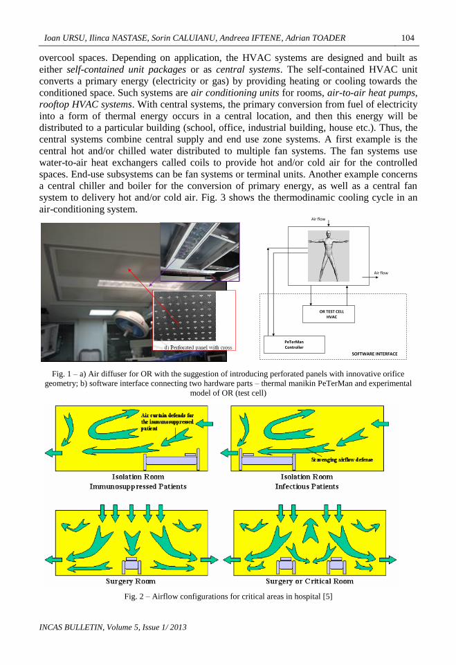
increasingly sophisticated control systems. Like in the project referred to [4], project which
aims to improve air quality in hospital operation rooms (ORs) [5] (Figs. 1, 2), the HVAC
systems can address specific objectives involving fluid dynamics, such as impinging jet
ventilation strategy [6]-[8]. In other cases, such as a metro system or in the skyscrapers
with hundred floors, it is necessary to have a complete air conditioning system, which could
keep the temperature, humidity or pressure within acceptable ranges.
The most HVAC systems are typically set to operate at designed conditions defined by
thermal loads. Without a robust control law, the system will become unstable, because the
actual thermal loads are time-varying and consequently the HVAC system would overheat or
DOI: 10.13111/2066-8201.2013.5.1.11
Ioan URSU, Ilinca NASTASE, Sorin CALUIANU, Andreea IFTENE, Adrian TOADER 104
INCAS BULLETIN, Volume 5, Issue 1/ 2013
overcool spaces. Depending on application, the HVAC systems are designed and built as
either self-contained unit packages or as central systems. The self-contained HVAC unit
converts a primary energy (electricity or gas) by providing heating or cooling towards the
conditioned space. Such systems are air conditioning units for rooms, air-to-air heat pumps,
rooftop HVAC systems. With central systems, the primary conversion from fuel of electricity
into a form of thermal energy occurs in a central location, and then this energy will be
distributed to a particular building (school, office, industrial building, house etc.). Thus, the
central systems combine central supply and end use zone systems. A first example is the
central hot and/or chilled water distributed to multiple fan systems. The fan systems use
water-to-air heat exchangers called coils to provide hot and/or cold air for the controlled
spaces. End-use subsystems can be fan systems or terminal units. Another example concerns
a central chiller and boiler for the conversion of primary energy, as well as a central fan
system to delivery hot and/or cold air. Fig. 3 shows the thermodinamic cooling cycle in an
air-conditioning system.
Air flow
Air flow
OR TEST CELL HVAC
Controller
PeTerMan Controller
SOFTWARE INTERFACE
Fig. 1 – a) Air diffuser for OR with the suggestion of introducing perforated panels with innovative orifice
geometry; b) software interface connecting two hardware parts – thermal manikin PeTerMan and experimental
model of OR (test cell)
Fig. 2 – Airflow configurations for critical areas in hospital [5]

105 Intelligent control of HVAC systems. Part I: Modeling and synthesis
INCAS BULLETIN, Volume 5, Issue 1/ 2013
In this paper we are above all interested in HVAC control synthesis. Generally speaking,
each HVAC system has its own control strategy. In this paper we propose a strategy that we
consider most appropriate, given the history of the field and our own experience. A
considerable amount of literature has been published on HVAC control synthesis. The
development of these technological systems − whose importance has significantly grown
since the oil crisis of the 1970’s − closely follows the history of automatic control over the
last six decades. An excellent survey on HVAC control systems can be found in [10]. Very
simplified, the HVAC control methodes can be classified into conventional/classical
techniques, also called hard control methods [10] (Proportional-Integral-Derivative-PID
control, Linear Quadratic Regulator-LQR, adaptive control, Lyapunov-based nonlinear
control etc.) and nonconventional artificial intelligence based techniques, also called soft
control methods [10] (fuzzy logic control, neural network control, agent-based intelligent
control systems etc.). It should be noted that overlapping of these categories is inevitable.
Fig. 3 – The schematic view of chilled water air-conditioning system with water-cooled condenser [9]
The conventional methods have their background in automatic control theory. Basically,
any classical control law synthesis starts from a mathematical model of the system, usually
called state model. In the online control process, the inputs and the feedbacks from the
previous system state are used by the control algorithm to optimize the control of the system
in the next time step. But the classical control laws have been synthesized/designed based on
mathematical models, and their weakness lies right here: due to inherent modeling limits,
burdened with measurement noises and incomplete observations of the state, the control of
complex processes becomes a really difficult task. Therefore, the classical control, based on
mathematical models, remains vulnerable to inaccurate and noisy inputs or feedbacks, even
after a history of over six decades. It seems strange that over 95% of the control algorithms
belong to prehistoric PID control [11]. It should be said however that this surprising outcome
can be also made in connection with the well known schism, invoked more than once [12],
between theoreticians and practitioners in the field.
2. A PHYSICAL MODEL OF HVAC SYSTEM
To illustrate our HVAC control technique, let us consider the single-zone/space HVAC physical model described in [2], often used as benchmark problem in the field (78 citations
on Google currently; e.g., [13], [14]). Fig. 4 refers to the system operating on the cooling
mode (air-conditioning). In all its details, the system components include thermal space,
heating/cooling coil, humidifier/dehumidifier, mixing box, air filter, supply and return fans,
filters, dampers, and ductwork.

Ioan URSU, Ilinca NASTASE, Sorin CALUIANU, Andreea IFTENE, Adrian TOADER 106
INCAS BULLETIN, Volume 5, Issue 1/ 2013
Operations performed in the system will be reflected in mathematical modeling (section
3). In this system, fresh air enters and mixes with 75% of the return air (position 5) at the
flow mixer (position 1), and remaining air is exhausted. The purposes of comfort anf hygiene
are considered in this system-to-fresh-air volumetric flow-rate ratio. Then, mixed air passes
through the heat exchanger components and finally by supply fan enters the thermal space as
supply air (position 2), to offset (compensate) the sensible (actual heat) and latent (humidity)
heat thermal loads acting upon the system; specifically, by changing of thermal load, the
system controller simultaneously varies volumetric flow rate of air and water, so that the
desired setpoints in temperature and relative humidity are maintained. Finally, the air in the
thermal space is drawn through a fan (position 4), 75% of this air gets recirculated and the
rest is exhausted from the system.
Some remarks from Wikipedia are given below for a quick understanding of the
concepts. An air conditioner is designed to change the air temperature and humidity within
an area (used for cooling and sometimes heating, depending on the air properties at a given
time). The cooling is typically done using a simple refrigeration cycle, but sometimes
evaporation is used, commonly for comfort cooling in buildings and motor vehicles. In
construction, a complete system of heating, ventilation and air conditioning is referred to as
"HVAC".
Ventilating is the process of "changing" or replacing air in any space to provide high
indoor air quality (i.e. to control temperature, replenish oxygen, or remove moisture, odors,
smoke, heat, dust, airborne bacteria, and carbon dioxide). Ventilation is used to remove
unpleasant smells and excessive moisture, introduce outside air, to keep interior building air
circulating, and to prevent stagnation of the interior air.
A fan is a machine used to create flow within a fluid, typically a gas such as air. Fans
produce air flows with high volume and low pressure (however higher than ambient
pressure), as opposed to compressors which produce high pressures at a comparatively low
volume.
Fig. 4 – HVAC system operating on the cooling mode, as air-conditioning system – schematic view [2]
3. MATHEMATICAL MODEL
In this Section, the construction of the mathematical model is performed with only a view to
obtain a framework of HVAC fuzzy logic controller validation by numerical simulations.
The controller design will be described in the next Section. The constitutive assumptions of
the mathematical model are the following [2]: 1) ideal gas behavior; 2) perfect mixing; 3)
constant pressure process; 4) negligible wall and thermal storage 5) negligible thermal losses
between components; 6) negligible infiltration and exfiltration effects; and 7) negligible

107 Intelligent control of HVAC systems. Part I: Modeling and synthesis
INCAS BULLETIN, Volume 5, Issue 1/ 2013
transient effects in the flow splitter and mixer. We introduce the following notations for
system’s parameters, constants and variables: − air mass density [kg/m3];
wh − enthalpy of
liquid water [J/kg]; wh − variation of enthalpy of water vapor [J/kg];
wvh − enthalpy of
water vapor [J/kg]; oW − humidity ratio of outdoor air; 2W − humidity ratio of supply air;
3W t − humidity ratio of thermal space; heV − volume of heat exchanger [m3]; pc − specific
heat of air [J/(kg o C )]; oT t − temperature of outdoor air [ o C ]; 2T t − temperature of
supply air [ o C ]; 3T t − temperature of thermal space [ o C ]; 3V − volume of thermal space
[m3]; M − humidity (moisture) load [kg/s]; Q − sensible heat load [W];
aq − volumetric
flow rate of air [m3/s];
wq − flow rate of chilled/heated water [m3/s]. We so specify that the
air with temperature oT t and flow rate aq t passes through the heat exchanger where an
amount of heat is exchanged with the air. Since we have the assumption of perfect mixing,
the air temperature within and exiting the heat exchanger is 2T t , which represents the
supply air temperature. Obviously, the air and the heat exchanger capacitance must be taken
into account, hence the resulting temperature has a transient response. After being cooling or
heating in the heat exchanger, the air at temperature 2T t passes into the thermal space with
the help of fan and the air temperature in the thermal space is 3T t . Consistenly with the
made assumptions, the effect of variations in instantaneous airspeed pressure zones is
neglected. There is no air leakage except exhaust valve areas.
The air flow in thermal space is homogeneous. The heat load Q in the thermal space
and the heat input heQ in the heat exchanger (positive for heating and negative for cooling)
are considered. Thermal losses between components are neglected and, thus, temperatures in
the locations 4 and 5 (Fig. 3) are equal to the temperature of the air exiting the thermal space.
Given that the infiltration and exfiltration effects are neglected, the flow rates at locations 2-
3 are equal to aq t .
The mathematical modeling is based on the energy conservation principle. For
simplicity, we neglect a moment the effects of humidity. Consider the basic relationship
pQ t mc T (1)
relating the amount of heat Q t absorbed by a mass m having specific heat pc to achieve a
temperature change T in the time interval t . Physically, the temperature variation implies
a transient regime and so, given the air mixture assumed in Section 3, the dynamics of
temperatures in the two key locations 2-3 are configured like this:
23 2
33 2 3
0.25 0.75he p p a o he
p a p
dTV c c q T T T Q
dt
dTV c q c T T Q
dt
(2)
Next, add a simple dynamic model of air humidity and a completion of thermal loads. Thus,
the differential equations describing the dynamic behavior of the HVAC system in Fig. 3 can
be written as follows:

Ioan URSU, Ilinca NASTASE, Sorin CALUIANU, Andreea IFTENE, Adrian TOADER 108
INCAS BULLETIN, Volume 5, Issue 1/ 2013
3 2 3 2 3
3 3 3
3 2 3
3 3
3 2
2 3 2
1
0.25 0.750.25 0.75
a wv awv
p p
a
a o a w w wo
he p he p he
q h qT T T W W Q h M
V c V c V
q MW W W
V Vq T T T q h h q
T W W WV c V c V
(3)
Indeed, in the right side of the first equation of (4), we observe a thermal load term generated
by the enthalpy of the water vapors, namely 2 3wv ah q W W ; then, we have a second
thermal load term wvh M , in which the moisture mass is directly involved; and, finally, a
third thermal load term defined by the sensible heat load Q (simply, the sensible heat is in
connection with the amount of heat required to increase or decrease the temperature of an
object or space, without changing its state of aggregation; latent heat is the amount needed to
change its aggregation state).
All these terms are linearly concatenated based on the principle of superposition of
effects. Now, it is easy to see how the other two equations are similarly obtained. As for the
signs of the thermal load terms, plus or minus, these signs indicate the influence on state
variables 2T t , 3T t , 3W t . For instance, the negative term wvh M contributes to the
decreasing of the temperature 3T t , and so on. It should be added that the actuators dynamics
have been neglected.
4. THE PROBLEM OF HVAC SYSTEM SYNTHESIS
There are two objectives of a quality HVAC system: thermal comfort represented herein by
the state variables of the thermal space 3T t , 3W t and energy savings. Most conventional
HVAC systems are based on a single rotational speed of the fan/compressor. A system with
variable speed control can control the heating/cooling capacity by changing the rotational
speed of the fan/compressor for load matching and thermal comfort; therefore it must be
complemented with a good control algorithm, to maintain comfort under any thermal loads.
In other words, the rotational speed of the fan, which in our case is proportional to the
volumetric flow rate of air aq , must be conceived as a control variable; similarly must be
considered the flow rate of chilled/heated water wq . This control strategy characterize the
HVAC system as a variable-air-volume system (VAV) that results in the lowest energy
consumption.
Fig. 5 − Feedback control system: standard block-diagram
P
C
z
y u
d

109 Intelligent control of HVAC systems. Part I: Modeling and synthesis
INCAS BULLETIN, Volume 5, Issue 1/ 2013
In fact, the system (3) is the mathematical model of a feedback control system (Fig. 5).
In the figure, P represents the physical system to be controlled, C and d the mathematical
models of the controller and the external disturbance at the output of the plant, respectively.
z represents a regulated/quality output. Further on, usual notations concern the state vector
x characterizing the plant P , the measurement output vector y , and the control vector u . In
our problem the two quantities z and y coincide. In this context, we will rewrite the system
(3) by introducing the variables in usual state form
1 3 2 3 3 2
1 3 2 3
1 2
1 2
: , : , :
: , :
: , :
: , :
a w
x T x W x T
y T y W
u q u q
d Q d M
(4)
This means that the effort to build a controller is based on measuring the two states
characterizing thermal space. With simplified notations for parameters and constants
1 2 3 4 1 2 3
3 3 3 3
1 1 1 1, , , , , ,wv w w
p p he p he p he
h h h
V c V c V V V c V c V
(5)
one obtains
1 1 3 1 1 2 2 2 1 3 1 2
2 1 2 2 1 4 2
3 1 1 3 1 1 1 1 3 2 2 1 2 2
1 1 2 2
0.25 0.25 0.75
,
wv
o o
x x x u W x u d h d
x W x u d
x x x u T x u W x W u u
y x y x
(6)
For the sake of compliance, we mention that the feedback systems are characterized by
two basic paradigms: the regulator, or stabilization system, and the tracking system [15],
[16]. The HVAC system is essentially a regulator: the controller goal is that to maintain the
thermal space temperature 1x and humidity ratio 2x at a certain set point T
1 2
e ex xr , i. e., to
counteract the error signals T
1 1 2 2
e ex t x x t x (Fig. 6) (by Ta is denoted the transpose
to a vector/matrix a ). The HVAC control synthesis problem can be defined as follows
C P
d u
η
r y
Fig. 6 − Basic configuration of a stabilization system

Ioan URSU, Ilinca NASTASE, Sorin CALUIANU, Andreea IFTENE, Adrian TOADER 110
INCAS BULLETIN, Volume 5, Issue 1/ 2013
Suppose that variations occur in the ambient temperatureoT , the humidity ambient ratio
oW ,
the humidity ratio of supply air 2W and the thermal loads Q , M from a certain equilibrium
point 2, , , ,e e e e e
o oT W W Q M which is in connection with a certain state equilibrium
1 2 3, ,e e ex x x . Provide an output feedback control law t t:u u y that brings the state
1 2,x t x t to the equilibrium point 1 2,e ex x . More specifically, the regulated (measured,
herein) output T
1 2( )=t x t x ty is required to approach the equilibrium point
1 2,e ex x .
It is known in the literature and in the practice of the field that the difficulty of solving
the problem is especially amplified in the presence of the thermal load changes
(disturbances d ) [2] and of inherent measurement noise η (Fig. 6). To specify, we write the
system [7] as model in variations by introducing the equilibrium point , ,e e ex u d
1 1 1 2 2 2 3 3 3
1 1 1 2 2 2 1 1 1 2 2 2
, ,
, , ,
e e e
e e e e
x x x x x x x x x
u u u u u u d d d d d d
(7)
Substitute (7) in (6) and consider the definition of the equilibrium point as that solution of
the system (6) that cancels the right-sides in the first three equations (6)
1 1 3 1 1 2 2 2 3 1 2
1 1 2 2 4 2
1 1 1 3 1 1 1 1 3 2 2 2 2
0
0
0 0.25 0.25 0.75
e e e e e e e ewv
e e e e
e e e e e e e e e e eo o
u x x u W x d h d
u W x d
u x x u T x u W x W u
(8)
A bilinear system in variations is obtained in matrix-form
3
0 01
,i i di
x x
u uA x B B E y = C x (9)
where
0 0 01 1 2 1 1 1
00 1 1
0 0 01 1 3 1 1 1
0 0
0.75 0.75
u u u
u
u u u
A
0 0 01 3 1 2 2
00 1 2
2
0
0
0
B
s
s
x x W x
W x3 3
400 0
fgh
E
1 2 1
1 2 1 3
1 13
0 0 01 0 0
0 0 , 0 , 0 0 ,0 1 0
0.75 0 00.75 0B B B C
(9')

111 Intelligent control of HVAC systems. Part I: Modeling and synthesis
INCAS BULLETIN, Volume 5, Issue 1/ 2013
A principle of parsimony, taken and used in systems identification [17], can be also
invoked in mathematical modeling. This philosophical principle says that entities should not
be multiplied needlessly; the simpler of two competing theories is to be preferred. The
mathematical model of the system, as it was obtained in (6), proved to be a parsimonious
one, that is neither too simple nor too complicated, so ultimately credible [2], [13], [14],
[18]. Indeed, the model is bilinear, so positioned as mathematical complexity between
linearity and nonlinearity. In terms of validation of an intelligent control strategy (based on
fuzzy logic, neural, networks) the model is so representative. However, it should be added
that an intelligent control strategy is largely free of mathematic model, as such its validation
in process, on-line, depends on preliminary validation on model only to a small extent.
We said in Section 2 that we will use the numerical data provided in [2] as reference
data for the proposed herein synthesis method. In order to transcribe the data from [2] in SI
units were used information from sites [19] and [20]. These numerical values resulted as
follows:
the nominal operating conditions, including the thermal loads:
29.44 CeoT ; 0.018e
oW ; 2 0.007eW ; 1 84960 Wed ; 2 0.02092 kg/sed ;
31 8.023 m /s eu ;
32 0.365 m /seu
constructive and functional HVAC system data base: 31.19 kg/m ; o1005 J/ kg Cpc ; 31.719 mheV ; 3
3 1655.115mV ; 2431700 J/kgwvh at
(see [19]); 53450 J/kgwh at 3 12.77 Cex (see [19]).
The analytical term w w p heh q c V in the system (3) is a generalization of the
corresponding analytical-numerical term 6000gpm p hec V in the original model given in
[2], in which the coefficient 6000 is physically dimensional. Data of [2] were converted
herein in SI units. Substituting these data in the system (8) and choosing 10000 J/kgwh ,
an equilibrium state 1 2 321.4855 C, 0.0091725, 12.631 Ce e ex x x very close to that given
in [2], 1 21.66 C (71 F)ex , 2 0.0092ex , 3 12.77 C (55 F)ex , was obtained.
In developing the mathematical model (6), the actuator dynamics were neglected. The
above discussion on the equilibrium points is not affected by this simplification. Therefore,
the control signals can be implemented using a simple dynamic model of order one
1G s z s u s k s (10)
5. ARTIFICIAL INTELLIGENCE BASED CONTROL OF HVAC SYSTEM
As already has been stated, the methods of the artificial intelligence in the solution of the
control problems are based in principle only on the input-output data of the process.
Therefore, herein the mathematical models (6) or (9) will serve only as illustration of
applying an artificial intelligence based control strategy. In the case of physical process, the
mathematical model is naturally substituted by the physical system.
In this paper we consider a neuro-fuzzy strategy [22], [23] for the HVAC system
control. It has two components: a) a neuro-control and b) a fuzzy logic control supervising
the neuro-control to counteract the saturation. To generate the two control signals − the
volumetric flow rate of air and the flow rate of chilled/heated water −, an elementary

Ioan URSU, Ilinca NASTASE, Sorin CALUIANU, Andreea IFTENE, Adrian TOADER 112
INCAS BULLETIN, Volume 5, Issue 1/ 2013
perceptron scheme [24], [25] is considered sufficiently efficient (Fig. 7). The elementary
perceptron is a unilayered neural network with a single neuron. For simplicity, we use a
generic notation u for the two control signals 1u and 2u . In the figure, T
1 2[ ] is the
weighting vector of the neural network, which is “trained” online by the gradient descent
learning method to reduce the cost J
2 2 21 1 2 2
1 1
1 1:
2 2
n n
nci i
J q e i e i q u i J in n
(11)
1 2,q q are weights on the cost and : ncu u is the provided neuro-control signal
1 1 2 2: ncu u e e (12)
From the system’s view point, the input is ncu and the output is 1 2,e ee . From neuro-
control training viewpoint, the system performance is assessed by the cost function, a
criterion supposing a trade-off between the first input 1e the tracking error, the second
input component 2e the rate of change of tracking error, and the control ncu . In fact, the
procedure (12) generates two neuro-control signals based on the sets of errors
1 1 1 2 1
1 2 2 2 1
: ,
: ,
t ref t t
h ref h h
e x x e e
e x x e e
(13)
where 1refx and 2refx are reference inputs (commands); in the case of the tracking systems,
these are time variable signals. Consequently, the update is given by the expression
1 2 1 2
( 1) ( ) ( )
( ) ( ) ( ) ( )( ) : diag( , ) diag( , )
( ) ( ) ( ) ( ) ( )
n
i n N
n n n
J J i i J i u in
n i u i u i i
e
e
(14)
In the relation (14), the matrix 1 2diag( , ) introduces the learning scale vector, ( )n is
the weight vector update and N marks a back memory (of N time steps). The derivatives in
(14) require only input-output information about the system. ( ) / ( )i i e u is online
approximated by the relationship
( ) / ( ) ( ( ) ( 1)) / ( ( ) ( 1))i i i i i i e u e e u u (15)
To counteract the risk of the neuro-control saturation and to achieve the enhancement of
the learning system, a fuzzy supervised neuro-control (FSNC) was developed in [22], [23]. It should be emphasized that for fast systems, such as the hydraulic servomechanisms, with
time constants in value of tenths of a second, the procedure has given good results. This time
NC
1e
2e
v 1
v 2 u
Fig. 7 − Perceptron type neuro-control

113 Intelligent control of HVAC systems. Part I: Modeling and synthesis
INCAS BULLETIN, Volume 5, Issue 1/ 2013
we consider the application of the idea in the case of a slow system, such as the HVAC
system. This means that the neuro-control switches to a Mamdani type fuzzy logic control
whenever the just described neuro-control is saturated. In this way, the two components
mutually complete a strategy with valences of optimality (neuro-control) and operational
safety (fuzzy control). The mathematical foundations of the approximations with neural
networks were laid in the paper of Cybenko [26]. Similarly, a new topic − fuzzy theory −, is
born with the work of Zadeh [27]. The ideas of fuzzy set and fuzzy control are introduced
with the aim to control the systems that are structurally difficult to model. Then, the fuzzy
control has been extensively studied and applied, in the Mamdani linguistic variant, begining
with the reference paper [28].
The three well-known components of the fuzzy control − fuzzyfier, fuzzy reasoning, and
defuzzyfier − will be succinctly described below. The fuzzyfier component converts the crisp
input signals
1k 2k, , 1, 2, ...e e k (16)
into their relevant fuzzy variables (or, equivalently, membership functions, MFs) associated
to the following set of linguistic terms: “zero” (ZE), “positive or negative small” (PS, NS),
“positive or negative medium” (PM, NM), “positive or negative big” (PB, NB) (for the sake
of simplicity, the most natural and unbiased membership functions are chosen, of triangular
and singleton type, Fig. 8). All MFs are defined on the common interval 1,1 . This means
that previously have been defined some scale factors (SFs) 1 2, ,
fe e uk k k for all
variables 1 2, , fe e u , respectively. The selection of suitable values for thes SFs involves
apriori knowledge about the process, but also can be done through trial and error to achieve
the best possible control performance. In principle, there is no well-defined method for good
setting of SF’s for FLC’s. Special attention should be paid to compute on-line the effective
SF of the control, (see below). Thus the relationships between the SFs and the input and
output variables of the self-tuning FLC are as follows
1 21N 1 2N 2 N, ,fe e f ue k e e k e u k u (17)
The fuzzy reasoning is defined by a fixed set of control rules (or, rules base, RB),
normally derived from experts’ knowledge. For instance, in the tracking control, the
construction of a rules base embodies the idea of a (direct) proportion between the error
signal 1e and the required fuzzy control fu [22], [23], [29]. In this case, of a regulator type
1 2/3 1/3 0 1/3 2/3 1 e1 ; e2
A(e1); B (e2)
NB NM NS ZE PS PM PB 1
a)
Fig. 8 −Membership functions for: a) scaled input variables y1, y2 and b) scalled fuzzy control uf
-1 -2/3 -1/3 0 1/3 2/3 u
1 uf
C (uf) NB NM NS 1 ZE PS PM PB
b)

Ioan URSU, Ilinca NASTASE, Sorin CALUIANU, Andreea IFTENE, Adrian TOADER 114
INCAS BULLETIN, Volume 5, Issue 1/ 2013
controller, the approach in the construction of the rules base is different. We specify that
there is a booming literature of the field, but especially we highlight the papers [30]-[32].
Observe that there is no consensus in the literature on the terminology used in describing
various types of fuzzy controllers. A fuzzy logic controller (FLC) is called adaptive if any
one of its tunable parameters (SFs, MFs, and rules base) changes when the controller is being
used, otherwise it is a nonadaptive or conventional FLC. An adaptive FLC that tunes an
already working controller by modifying either its MFs or SFs or both of them is called a
self-tuning FLC. If a FLC is tuned by automatically changing its RB, then it is called a self-
organizing FLC [33].
2e
1e
fu NB NM NS ZE PS PM PB
a)
NB NB NB NB NM NS NS ZE
NM NB NM NM NM NS ZE PS
NS NB NM NS NS ZE PS PM
ZE NB NM NS ZE PS PM PB
PS NM NS ZE PS PS PM PB
PM NS ZE PS PM PM PM PB
PB ZE PS PS PM PB PB PB
1e
2e
NB NM NS ZE PS PM PB
b)
NB VB VB VB B SB S ZE
NM VB VB B B MB S VS
NS VB MB B VB VS S VS
ZE S SB MB ZE MB SB S
PS VS S VS VB B MB VB
PM VS S MB B B VB VB
PB ZE S SB B VB VB VB Fig. 9 − a) Rules base for computation of fu ; b) rules base for computation of updating factor [30]
A conventional FLC of Proportional Derivative (PD)-type will be first described. This
totals a number of n = 77 IF..., THEN... rules, that is the number of the elements of the
Cartesian product AB, A = B: = {NB; NM; NS; ZE; PS; PM; PB}. These sets are associated
with the sets of linguistic terms chosen to define the membership functions for the fuzzy
variables 1e and, respectively, 2e . The structure of the n rules is shown in Fig. 9 a). Let T be the
discrete sampling time. Consider the two scaled (normalized) input crisp variables e1Nk and
e2Nk, at each time step kt kT (k = 1, 2,...). Taking into account the two ordinates
corresponding in the figure to each of the two crisp variables, a number of M 22
combinations of two ordinates must be investigated. Having in mind these combinations, a
number of M if..., then... rules will operate in the form
1N 2N Nif is and is , then is , 1, 2,...,k i k i f k ie A e B u C i M (18)
(Ai ,Bi ,Ci are linguistic terms belonging to the sets A, B, C, and A = B = C, see Fig. 9a). Note
that RB in Fig. 9a) characterizes the requirements involving a two-dimensional phase plane,

115 Intelligent control of HVAC systems. Part I: Modeling and synthesis
INCAS BULLETIN, Volume 5, Issue 1/ 2013
so that the conventional FLC drives the system into the so-called sliding mode [34]. A self-
tuning FLC is obtained by online updating the control gain . This serves to counteract the
controller overshoot and to improve the overall control performance. RB for depends on
each process, and of each “rough” RB operating, in this case of the one given in Fig. 9a). RB
shown in Fig. 9b) is used in [30], with applications which gave good results on theoretical
mathematical models. The new associated linguistic terms are “very small” (VS), “small”
(S), “small big” (SB), “medium big” (MB), “big” (B), “very big” (VB).
It is worthy to note that the authors of the paper [30] present in [31] a new application,
this time on HVAC systems and another RB for control gain was obtained.
2e
Pk NB NS ZE PS PB
NB PVB PVB PVB PB PM
NS PVB PVB PB PB PM
1e ZE PB PB PM PS PS
PS PM PS PS PS PS
PB PS PS ZE ZE ZE a)
2e
Dk NB NS ZE PS PB
NB ZE ZE PS PS PB
NS ZE ZE ZE ZE PS
1e ZE ZE ZE ZE PS PB
PS PS PS PS PB Z
PB ZE ZE ZE PS PB b)
2e
Ik NB NS ZE PS PB
NB PVB PB PM PM PM
NS PVB PB PB PM PS
1e ZE PM PS ZE ZE ZE
PS PM PM PS ZE ZE
PB PS ZE ZE ZE ZE c)
Fig. 10 − Rules base for self-tuning a PID-type fuzzy adaptive control: a) Pk ; b) Ik ; c) Dk
Other authors [32] consider as a starting point in the synthesis of a self-tuning FLC the
well-known relationship which defines a Proportional-Integral-Derivative (PID) control
1
1k
P I Di
u k k e k k e i k e k e k
(19)
The coefficients Pk , Ik , Dk are usually tuned according to certain criteria of classical
synthesis [35], [36], [32]. RB shown in Fig. 10 is used in [32].

Ioan URSU, Ilinca NASTASE, Sorin CALUIANU, Andreea IFTENE, Adrian TOADER 116
INCAS BULLETIN, Volume 5, Issue 1/ 2013
Fig. 11 − Sketch of the fuzzy supervised neural-control (FSNC)
The defuzzyfier concerns just the transforming of these if …, then rules into a
mathematical formula giving the output control variable uf. In terms of fuzzy logic, each rule
of the form (18) defines a fuzzy set AiBiCi in the input-output Cartesian product space R3,
whose membership function can be defined in the manner
1 2min[ ( ), ( ), ( )], 1, ... , , ( 1, 2, ...)i i iA k B k Ce e u i M kui
(20)
For simplicity, the singleton-type membership function C(u) of control variable has been
preferred; in this case, ( )iC u will be replaced by ui
0 , the singleton abscissa. Therefore,
using 1) the singleton fuzzyfier for uf, 2) the center-average type defuzzyfier, and 3) the min
inference, the M if..., then… rules can be transformed, at each time step k, into a formula
giving the crisp control u f [37], [38]
M
i
M
iuiuf ii
uu1 1
0 / (21)
neurocontrol
performance
Physic. system/
mathem. model
perturbations
fuzzysupervisor
fuzzy supervised neurocontrol
- FSNC
u
expertise
preliminary
knowlegde
fuzzy inference
defuzzyfication
fuzzyfication
u
uf
. . . . . . .
unc
Selection /
switching law
Y1 Y2 Yn
reference r +
Y Y
u
Ju
uuYJJ
umin:
,
Yu
J
Yu
n
n
, ,Y F Y u
uYFY ,,
u

117 Intelligent control of HVAC systems. Part I: Modeling and synthesis
INCAS BULLETIN, Volume 5, Issue 1/ 2013
The FSNC operates as fuzzy logic control fu in the case when neuro-control nu saturated.
In the case of fuzzy control operating, the fuzzy neuro-control nu is concomitantly updated
in the context of the real acting fuzzy control fu . To obtain the rigor and accuracy of
regulated process tracking, fuzzy logic control switches on neuro-control whenever
readjusted neuro-control nu is not saturated. At time st , when the switching from fuzzy logic
control to neuro-control occurs, the readjusted weighting vector r will be derived by
considering a scale factor nf uu [38]
1r 2 2 1 2r 2,f f nc f ncu y u u y u u
The aforementioned FSNC was brought to the proof in various numerical simulations
reported in [22], [23], [25], [38], and also in laboratory tests [29], [39]. A sketch of the
FSNC is shown in Fig. 11.
5. CONCLUDING REMARKS
The mathematical model described in Section 3 is one of the most commonly HVAC models
referenced in literature. Therefore, it will be used, in a second part to this paper, as a
benchmark for the numerical simulation study of a special control strategy called FSNC
(Fyzzy Supervised Neuro-Control). It must be said that, although independent of a
mathematical model of the controlled system, the intelligent control requires a careful
evaluation by numerical simulations, especially with regard to the adoption of the component
“rules base”. We mention also that the results of this study will serve as a starting point in
the development of the project [4].
Acknowledgements. The authors gratefully acknowledge the financial support of the
GRANT UEFISCDI-CNCS ROMANIA No. PN-II-PT-PCCA-2011-3.2-1212.
REFERENCES
[1] M. S. Imbabi, Computer validation of scale model tests for building energy simulation, Int. J. Energy Res.,
vol. 14, pp. 727–736, 1990.
[2] B. Argüello-Serrano, M. Velez-Reyes, Nonlinear control of a heating, ventilating and air conditioning systems
with thermal load estimation, IEEE Transaction on Control Systems Technology, vol. 7, no. 1, pp. 56-63,
1999.
[3] F. Scotton, Modeling and Identification for HVAC Systems, Thesis, Royal Institute of Technology KTH,
Stockholm, Sweden, 2012.
[4] *** Advanced strategies for high performance indoor Environmental QUAliTy in Operating Rooms –
EQUATOR, UEFISCDI-CNCS Project No. PN-II-PT-PCCA-2011-3.2-1212.
[5] E. E. Khalil, Air-conditioning systems’ developments in hospitals: comfort, air quality, and energy utilization,
http://www.inive.org/members_area/medias/pdf/Inive%5Cclimamed%5C85.pdf
[6] T. Karimipanah, H. B. Awbi, Theoretical and experimental investigation of impinging jet ventilation and
comparison with wall displacement ventilation, Building and Environment, vol. 37, pp. 1329-1342, 2002.
[7] Y. Cho, H. B. Awbi, T. Karimipanah, A comparison between four different ventilation systems, presented at
the International Conference Roomvent, Copenhagen, September 2002.
[8] A. Meslem, I. Nastase, F. Bode, C. Beghein, Optimization of lobed perforated panel diffuser: Numerical study
of orifices arrangement, Int. Journal of Ventilation, vol. 11, no. 3, pp. 255-270, 2012.
[9] *** Fundamentals of HVAC Controls, http://www.cs.berkeley.edu/~culler/cs294-f09/m197content.pdf
[10] A. Dounis, C. Caraiscos, Advanced control systems engineering for energy and comfort management in a
building environment – A review, Renew. Sust. Energ. Rev., vol. 13, pp. 1246-1261, 2009.
[11] K. J. Astrom, T. Hagglund, PID controllers: Theory, design, and tuning, 2nd edition, Instrument Society of
America. Research Triangle Park, NC, 1995.

Ioan URSU, Ilinca NASTASE, Sorin CALUIANU, Andreea IFTENE, Adrian TOADER 118
INCAS BULLETIN, Volume 5, Issue 1/ 2013
[12] J. C. Doyle, and G. Stein, Multivariable feedback design: concepts for a classical/modern synthesis, IEEE
Transactions on Automatic Control, vol. 26, pp. 4-16, 1981.
[13] E. Semsar, M. J. Yazdanpanah, C. Lucas, Nonlinear control and disturbance decoupling of an HVAC system
via feedback linearization and backstepping, IEEE Conference on Control Applications, vol. 1, pp. 646-
650, 2003.
[14] A. Parvaresh, S. M. A. Mohammadi, Adaptive self-tuning decoupled control of temperature and relative
humidity for a HVAC system, International Journal of Engineering and Science Research, vol. 2, no. 9,
pp. 900-908, 2012.
[15] B. D. O. Anderson, J. B. Moore, Optimal Control. Linear Quadratic Methods, Prentice Hall, 1989.
[16] I. Ursu, A. Toader, S. Balea, A. Halanay, New stabilization and tracking control laws for electrohydraulic
servomechanisms, European Journal of Control, vol. 19, no 1, 2013.
[17] T. Söderstrom, P. Stoica, System identification, Prentice-Hall, New York–London–Toronto–Sydney–Tokio,
1989.
[18] M. Mongkolwongrojn, V. Sarawit, Implementation of fuzzy logic control for air conditioning systems,
ICCAS 2005, June 2-5, KINTEX, Gyeonggi-Do, Korea.
[19] *** http://www.multithermcoils.com/pdf/conversion-factors.pdf
[20]*** http://ebookbrowse.com/tablas-si-moran-shapiro-fundamentals-of-engineering-thermodynamics-5th-
edition-con-r12-pdf-d419725143
[21] M.-L. Chiang, L.-C. Fu, Nonlinear and Switching Control for the HVAC System,
http://ntur.lib.ntu.edu.tw/retrieve/169729/64.pdf
[22] I. Ursu, F. Ursu, L. Iorga, Neuro-fuzzy synthesis of flight controls electrohydraulic servo, Aircraft
Engineering and Aerospace Technology, vol. 73, pp. 465-471, 2001.
[23] I. Ursu, I., G. Tecuceanu, F. Ursu Neuro-fuzzy control synthesis for electrohydraulic servos actuating
primary flight controls, 25th ICAS Congress, Hamburg, Germany, 3-8 September 2006,
http://www.icas.org/ICAS_ARCHIVE_CD1998-2010/ICAS2006/PAPERS/565.PDF
[24] V. Vemuri, Artificial neural networks in control applications. In Advances in Computers, edited by M. C.
Yovits, Academic Press, vol. 36, pp. 203-332, 1993.
[25] I. Ursu, Felicia Ursu, Active and semiactive control (in Romanian), Publishing House of the Romanian
Academy, 2002.
[26] G. Cybenko, Approximation by superpositions of a sigmoidal function, Control Signals Systems, vol. 2, pp.
303-314, 1989.
[27] L. A. Zadeh, Fuzzy sets, Information and control, vol. 8, pp.338-353, 1965.
[28] E. H. Mamdani, Application of fuzzy algorithms for the control of a simple dynamic plant, Proceedings of
the IEEE, vol. 121, no. 12, pp. 121-159, 1974.
[29] I. Ursu, G. Tecuceanu, F. Ursu, R. Cristea, Neuro-fuzzy control is better than crisp control, Acta
Universitatis Apulensis, no. 11, 259-269, 2006.
[30] R. K. Mudi, N. R. Pal, A robust self-tuning scheme for PI and PD type fuzzy controllers, IEEE Transactions
on Fuzzy Systems, vol. 7, no. 1, pp. 2-16, 1997.
[31] A. K. Pal and R. K. Mudi, Self-Tuning Fuzzy PI Controller and its Application to HVAC Systems,
International Journal of Computational Cognition, vol. 6, no. 1, pp. 25-30, 2008.
[32] S. Soyguder, M. Karakose, H. Alli, Design and simulation of self-tuning PID-type fuzzy adaptive control for
an expert HVAC system, Expert System with Applications, vol. 36, pp. 4566–4573, 2009.
[33] T. J. Procyk, E. H. Mamdani, A linguistic self-organizing process controller, Automatica, vol. 15, no. 1, pp.
53–65, 1979.
[34] R. Palm, Robust control by fuzzy sliding mode, Automatica, vol. 30, no. 9, pp. 1429–1437, 1994.
[35] K. L. Tang, R. J. Mulholland, Comparing fuzzy logic with classical controller designs, IEEE Transactions
on Systems Man and Cybernetics, vol. 17, no. 6, pp. 1085–1087, 1987.
[36] Z. Y. Zhao, M. Tomizuka, S. I. Isaka, Fuzzy gain scheduling of PID controllers, IEEE Transactions on
Systems, Man and Cybernetics, vol. 23, pp. 1392–1398, 1993.
[37] L.-X. Wang, H. Kong, Combining mathematical model and heuristics into controllers: an adaptive fuzzy
control approach, Proc. of the 33rd IEEE Conference on Decision and Control, Buena Vista, Florida,
December 14-16, vol. 4, pp. 4122-4127, 1994.
[38] I. Ursu, F. Ursu, Airplane ABS control synthesis using fuzzy logic, Journal of Intelligent and Fuzzy Systems,
vol. 16, no. 1, pp. 23-32, 2005
[39] I. Ursu, G. Tecuceanu, A. Toader, C., Calinoiu, Switching neuro-fuzzy control with antisaturating logic.
Experimental results for hydrostatic servoactuators, Proceedings of the Romanian Academy, Series A,
Mathematics, Physics, Technical Sciences, Information Science, 12, 3, 231-238, 2011.


![[O] cOmpaniessavarinocompanies.com/content/documents/bids... · hvac general notes hvac abbreviations hvac ductwork symbols hvac control symbols chaintreuil jensen stark architectural](https://static.fdocuments.us/doc/165x107/5ae5a13f7f8b9a29048c7dfa/o-compan-general-notes-hvac-abbreviations-hvac-ductwork-symbols-hvac-control-symbols.jpg)