VIRGINIA CENTER FOR TRANSPORTATION INNOVATION AND RESEARCH

530 Edgemont Road, Charlottesville, VA 22903-2454

www. VTRC.net

Integration of Travel Demand Models With Operational Analysis Tools

http://www.virginiadot.org/vtrc/main/online_reports/pdf/14-r5.pdf JIAQI MA

Graduate Research Assistant MICHAEL J. DEMETSKY, Ph.D., P.E. Henry L. Kinnier Professor of Civil & Environmental Engineering Department of Civil & Environmental Engineering University of Virginia

Final Report VCTIR 14-R5

Standard Title Page - Report on Federally Funded Project

1. Report No.: 2. Government Accession No.: 3. Recipient’s Catalog No.:

FHWA/VCTIR 14-R5

4. Title and Subtitle: 5. Report Date:

Integration of Travel Demand Models with Operational Analysis Tools

December 2013

6. Performing Organization Code:

7. Author(s):

Jiaqi Ma, and Michael J. Demetsky, Ph.D., P.E.

8. Performing Organization Report No.:

VCTIR 14-R5

9. Performing Organization and Address:

Virginia Center for Transportation Innovation and Research

530 Edgemont Road

Charlottesville, VA 22903

10. Work Unit No. (TRAIS):

11. Contract or Grant No.:

102608

12. Sponsoring Agencies’ Name and Address: 13. Type of Report and Period Covered:

Virginia Department of Transportation

1401 E. Broad Street

Richmond, VA 23219

Federal Highway Administration

400 North 8th Street, Room 750

Richmond, VA 23219-4825

Final Contract Report

14. Sponsoring Agency Code:

15. Supplementary Notes:

16. Abstract:

Continuing growth in urban travel demand inevitably leads to a need for more physical capacity within the transportation

system. However, limited financial resources, high construction costs, environmental considerations, long timelines, and an

increasingly complex regulatory process have essentially rendered capacity-adding projects to be actions of last resort. Before

such projects are undertaken, decision makers, planners, and engineers evaluate alternative operational improvement strategies

that can eliminate, mitigate, or forestall the need for a more traditional highway construction project. Effectively evaluating the

wide range of operational improvement strategies that are available is not a trivial matter, and this is particularly true when the

performance of such strategies is compared to the construction of new lanes.

The purpose of this study was to recommend methods to obtain input data for operational analysis tools that operate as

post-processors to travel demand models. Among all operational planning tools compatible with the four-step planning process,

the Florida ITS Evaluation (FITSEval) tool was selected to be integrated with the primary planning software used by the Virginia

Department of Transportation, i.e., Cube.

To achieve the objective of this study, methods for estimating peak period flows from travel forecasting model outputs

were investigated and Virginia data were examined for areas where planning forecasts and 24-hour travel patterns were available.

Relationships between peak period flows and 24-hour data were studied. Procedures for obtaining the time-of-day factors for

link and trip tables are provided using continuous count stations and National Household Travel Survey Data for Virginia.

The modeling process was demonstrated by two case studies for the Hampton Roads area where the latest travel demand

model was recently completed and many potential capacity enhancing operational strategies were available. Two case studies,

Incident Management systems and HOT lanes deployment, were evaluated, and the results of the base case and operational

strategy deployment scenarios were compared to make recommendations on the feasibility of the evaluated projects.

This report is designed to serve as a reference for users of FITSEval or similar operational analysis tools for evaluating

operational capacity enhancements.

17 Key Words: 18. Distribution Statement:

Operational analysis, travel demand modeling, travel forecasting No restrictions. This document is available to the public

through NTIS, Springfield, VA 22161.

19. Security Classif. (of this report): 20. Security Classif. (of this page): 21. No. of Pages: 22. Price:

Unclassified Unclassified 59

Form DOT F 1700.7 (8-72) Reproduction of completed page authorized

 

  

FINAL REPORT

INTEGRATION OF TRAVEL DEMAND MODELS WITH OPERATIONAL ANALYSIS TOOLS

Jiaqi Ma

Graduate Research Assistant

Michael J. Demetsky, Ph.D., P.E. Henry L. Kinnier Professor of Civil & Environmental Engineering

Department of Civil & Environmental Engineering

University of Virginia

VCTIR Project Manager Catherine C. McGhee, P.E.

Virginia Center for Transportation Innovation and Research

In Cooperation with the U.S. Department of Transportation Federal Highway Administration

Virginia Center for Transportation Innovation and Research (A partnership of the Virginia Department of Transportation

and the University of Virginia since 1948) Charlottesville, Virginia

December 2013 VCTIR 14-R5

 

ii  

DISCLAIMER

The project that is the subject of this report was done under contract for the Virginia Department of Transportation, Virginia Center for Transportation Innovation and Research. The contents of this report reflect the views of the authors, who are responsible for the facts and the accuracy of the data presented herein. The contents do not necessarily reflect the official views or policies of the Virginia Department of Transportation, the Commonwealth Transportation Board, or the Federal Highway Administration. This report does not constitute a standard, specification, or regulation. Any inclusion of manufacturer names, trade names, or trademarks is for identification purposes only and is not to be considered an endorsement.

Each contract report is peer reviewed and accepted for publication by staff of the Virginia Center for Transportation Innovation and Research with expertise in related technical areas. Final editing and proofreading of the report are performed by the contractor.

Copyright 2013 by the Commonwealth of Virginia. All rights reserved.

 

iii  

ABSTRACT

Continuing growth in urban travel demand inevitably leads to a need for more physical capacity within the transportation system. However, limited financial resources, high construction costs, environmental considerations, long timelines, and an increasingly complex regulatory process have essentially rendered capacity-adding projects to be actions of last resort. Before such projects are undertaken, decision makers, planners, and engineers evaluate alternative operational improvement strategies that can eliminate, mitigate, or forestall the need for a more traditional highway construction project. Effectively evaluating the wide range of operational improvement strategies that are available is not a trivial matter, and this is particularly true when the performance of such strategies is compared to the construction of new lanes.

The purpose of this study was to recommend methods to obtain input data for operational

analysis tools that operate as post-processors to travel demand models. Among all operational planning tools compatible with the four-step planning process, the Florida ITS Evaluation (FITSEval) tool was selected to be integrated with the primary planning software used by the Virginia Department of Transportation, i.e., Cube.

To achieve the objective of this study, methods for estimating peak period flows from

travel forecasting model outputs were investigated and Virginia data were examined for areas where planning forecasts and 24-hour travel patterns were available. Relationships between peak period flows and 24-hour data were studied. Procedures for obtaining the time-of-day factors for link and trip tables are provided using continuous count stations and National Household Travel Survey Data for Virginia.

The modeling process was demonstrated by two case studies for the Hampton Roads area

where the latest travel demand model was recently completed and many potential capacity enhancing operational strategies were available. Two case studies, Incident Management systems and HOT lanes deployment, were evaluated, and the results of the base case and operational strategy deployment scenarios were compared to make recommendations on the feasibility of the evaluated projects.

This report is designed to serve as a reference for users of FITSEval or similar

operational analysis tools for evaluating operational capacity enhancements.

 

  

FINAL REPORT

INTEGRATION OF TRAVEL DEMAND MODELS WITH OPERATIONAL ANALYSIS TOOLS

Jiaqi Ma

Graduate Research Assistant

Michael J. Demetsky, Ph.D., P.E. Henry L. Kinnier Professor of Civil & Environmental Engineering

Department of Civil & Environmental Engineering

University of Virginia

INTRODUCTION

In many urban areas where travel demand exceeds capacity, it is difficult to increase capacity through a physical expansion of the transportation system in a timely manner. Challenges include limited financial resources, environmental constraints, adverse impacts from the displacement of businesses and residences, and increased costs associated with urban work zones. Accordingly, operational strategies, such as the provision of travel information; the management of signal timings, and ramp metering, have received attention as they tend to have fewer adverse impacts and a shorter deployment time than traditional construction alternatives. Yet fully considering these alternatives within the planning process requires their evaluation at a high level of specificity as would be the case with a capacity expansion. For example, the goal of a traveler information system may be to reduce secondary incidents associated with routine queuing (e.g., a queue warning system on a freeway) or the goal may be to elicit a change in departure time (e.g., a web-based trip planning system). For each goal, the impact of the system on measures of effectiveness (MOEs) such as reliability (e.g., travel time variance), delay (e.g., vehicle hours of travel), safety (e.g., number of crashes), and air quality (e.g., pounds of nitrogen oxides) will need to be forecast so that the impact can be compared with a range of other alternatives. It is also possible to monetize these benefits, divide by the cost of the alternative, and compare the resulting benefit-cost ratio of a host of diverse alternatives. FHWA (2012) reports on three very different approaches that facilitate such computations for operations improvements. Sketch planning approaches use a spreadsheet format, can be implemented within a few weeks, do not require detailed network level data, and are suitable for screening a large number of alternatives; examples of sketch tools are Cal-BC (Booz-Allen & Hamilton Inc., 1999) and SCRITS (Science Applications International Corporation, 1999). A considerably more detailed approach is to integrate travel demand and microscopic simulation models; in direct contrast to sketch planning, these integrated models may necessitate a year to deploy, require detailed network level data, and, because of their expense and complexity, are most appropriate when an alternative has been selected and one is questioning various deployment options. Post-processing tools lie somewhere in between in

 

2  

terms of complexity and granularity. Such tools give a more informed evaluation than sketch planning approaches by using more detailed network level data and travel behavior elements of the travel demand model, but require more resources. Yet because these tools are designed to accept such detailed model data as inputs, they are not as resource intensive as an approach that requires microscopic simulation models. Examples of post-processors are the Florida ITS Evaluation (FITSEval) Tool (FDOT, 2008, 2012) and the ITS Deployment Analysis System (IDAS) (FHWA, 2001). Unfortunately, the format of the demand model outputs is often not consistent with the required inputs for any of the operational analysis models which focus on peak period conditions. Essentially, these models utilize the modal split and traffic assignment inputs from the traditional planning model, or require a loaded network input with operational strategies deployment to estimate changes in modal and route decisions of travelers resulting from operational strategies. Methods and best practices for translating the travel demand model outputs into inputs for operational tools are needed. Specifically, these inputs must represent specific times of the day so that peak periods and recurring congestion can be explicitly modeled, and trends in congestion growth established. Also, more detailed information on the peak Origin-Destination (O-D) flows, which show redistribution of equilibrium over multiple routes for peak-periods and time dependency of network characteristics, is desirable for accurate evaluations of potential operational strategies if re-estimation of network flows is needed. This is a research area that falls between model development and model applications as, typically, planners have concerns for the traditional planning process outputs and operational personnel have focused on the decisions concerning operational strategy deployments.

PURPOSE AND SCOPE

This study developed methods to extract input data from travel demand models that is suitable for operational analysis tools. The planning model outputs were examined for their ability to reflect peak period link volume or O-D adjustments. The scope of this study is limited to operational analysis tools that are sensitive to changes in travel route, mode, or time of departure and which are suitable for execution during the planning process.

METHODS

The following tasks were undertaken to achieve the objectives of this research. They differ from those originally stated in the proposal in that the former tasks 4, 5, 6 and 7 were combined as task 4 for more effective presentation of the work.

1. Review the Literature. The literature was reviewed to understand procedures of

benefit/cost (B/C) analysis for operational strategies and to identify operational analysis tools that are available for post-processing the results from transportation planning models to evaluate operational strategy deployment. Different tools were compared for their advantages and disadvantages in the performance of evaluation. Strategies for estimating the inputs for these operational analysis models were

 

3  

addressed through a rigorous examination of studies on the connection between travel demand models and operational analysis tools. Available tools were examined and real world practices, if any, were also reviewed to choose a suitable tool to be used in this research.

2. Select Planning and Operational Analysis Programs for the Study. The Cube

planning software as used by VDOT was used in this study for the transportation planning part so as to ensure compatibility for future VDOT use of this research. The models calibrated for a study area where good planning data are available were presented for application with a representative operational analysis tool. Since the Hampton Roads area has recently finished an update to the long-range transportation plan, it was selected as the case study area for this research. The operational analysis tool was selected based on the comparison results from the literature review.

3. Develop a Strategy for reflecting Peak Period Demand Adjustments from 24-hour O-

D Flows. Acknowledging that travelers’ routing strategies for peak periods can vary from the aggregated 24-hour O-D patterns, valid evaluations of operational strategies require best estimates of O-D flows during the periods of maximum effectiveness. In this regard, methods for estimating peak period flows from travel forecasting model outputs were investigated along with an examination of data from Hampton Roads where recent planning forecasts and 24-hour travel patterns are available. In the latter case, relationships between peak period flows and data for more generally available time periods were studied. A procedure for converting daily planning model outputs for period based input into the operational analysis tool was provided.

4. Demonstrate Modeling Process. The modeling process was demonstrated by two

case studies in the Hampton Roads area where the latest travel demand model was recently completed and many potential capacity enhancing operational strategies are available. The two case study projects, Incident Management systems and HOT lanes deployment, were evaluated separately and the results of the base case and operational strategy deployment scenarios are compared to make recommendation on the feasibility of the projects.

RESULTS AND DISCUSSION

Literature Review

The purpose of the literature review was multifold: to review the basic concepts of benefit/cost analysis, to review all the operational analysis tools for selecting an appropriate analysis tool, to determine how to convert daily volume to peak hour analysis, and to review case studies using related tools. Relevant literature was identified using the Transport Research International Documentation (TRID), a newly integrated database that combines the records from TRB’s Transportation Research Information Services (TRIS) Database and the OECD's Joint Transport Research Centre’s International Transport Research Documentation (ITRD) Database.

 

4  

Benefit/Cost Analysis

Most of the recent operational analysis tools use benefit/cost analysis to determine a project’s cost-effectiveness. Benefit/cost (B/C) analysis is defined as a systematic process for calculating and comparing the benefits and costs of a project to determine if it is a sound investment (justification/feasibility) and see how it compares with alternate projects (ranking/priority assignment) (FHWA, 2012).

Benefits in a B/C analysis are calculated by estimating the incremental change in various

MOEs and then applying an established value to the identified amount of change to monetize the benefit. MOEs can include a wide range of metrics depending on the anticipated impacts of the various projects being analyzed. The MOEs should be identified during the analysis set up, and should be sufficiently comprehensive to capture the full benefits (positive impacts) and disbenefits (negative impacts) of the identified projects. The MOEs might include travel time, crashes, fuel use, nonfuel vehicle operating costs, emissions/air quality and agency efficiency, etc. Operational Analysis Tools

Dozens of individual analysis tools and methodologies designed for conducting B/C analysis of one or more operational strategies have been identified to date. Some of the most widely distributed and applied tools used for conducting B/C analysis of operational strategies are summarized in Table 1 (FHWA, 2012). This listing includes those major tools developed by federal, state, or regional transportation agencies (or affiliated research organizations) that are available within the public realm. The MOEs produced by each of the tools are shown in Table 2.

These tools and methods can generally be segmented into three broad categories,

including the following (FHWA, 2012): 1. Sketch-planning methods. These analysis methods provide simple, quick, and low-

cost estimation of operational strategy benefits and costs. Often based in a spreadsheet format, these methods often rely on generally available input data and static default relationships between the strategies and their impact on a limited number of MOEs to estimate the benefits of the strategy. A number of established B/C tools, including TOPS-BC, SCRITS, and Cal-BC, are classified as sketch-planning methods; however, this category also includes scores of individually developed and customized spreadsheet and simple database methods configured to support various analyses by single agencies.

2. Post-processing methods. These methods are often more robust than sketch-planning

methods, as they seek to more directly link the B/C analysis with the travel demand, network data, and performance measure outputs from regional travel demand or

 

5  

Table 1. Summary of Existing B/C Analysis Tools (FHWA, 2012) Tool/Method Developed by Web Site Sketch Planning Tools BCA.net FHWA (1998) http://www.fhwa.dot.gov/infrastructure/ass

tmgmt/bcanet.cfm CAL-BC Caltrans (1999) http://www.dot.ca.gov/hq/tpp/offices/eab/L

CBC_Analysis_Model.html COMMUTER Model U.S. EPA (V2.0 2005) http://www.epa.gov/oms/stateresources/pol

icy/pag_transp.htm EMFITS New York State DOT (2004) https://www.nysdot.gov/divisions/engineer

ing/design/dqab/dqab-repository/pdmapp6.pdf

Highway Economic Requirements System – State Version (HERS-ST)

FHWA (V4.5 2011) http://www.fhwa.dot.gov/infrastructure/asstmgmt/hersindex.cfm

IMPACTS FHWA (1999) http://www.fhwa.dot.gov/steam/impacts.htm

Screening Tool for ITS (SCRITS)

FHWA (1999) http://www.fhwa.dot.gov/steam/scrits.htm

Tool for Operations Benefit/Cost (TOPS-BC)

FHWA (2012) N/A

Trip Reduction Impacts of Mobility Management Strategies (TRIMMS)

Center for Urban Transportation Research (CUTR) at the University of South Florida (2009)

http://www.nctr.usf.edu/abstracts/abs77805.htm

Post-processing Tools Surface Transportation Efficiency Analysis Model (STEAM)

FHWA (V2.0 2000) http://www.fhwa.dot.gov/steam/index.htm

IDAS FHWA (2003) http://idas.camsys.com The Florida ITS Evaluation (FITSEval) Tool

Florida DOT (2008) N/A

simulation models. Several established tools, including IDAS and the FITSEval application, have been designed to directly accept detailed model data as inputs to the analysis. The tools then provide additional analysis within their framework to assess impacts to MOEs outside the capabilities of typical travel demand models. Outside of these more established tools, these post-processing methods also include customized applications, algorithms, and routines that may be applied directly within a region’s existing modeling framework to produce the required MOEs. These methods are often more capable of assessing the impacts of route, mode, or temporal shifts than sketch-planning methods.

3. Multiresolution/multiscenario methods. These analysis methods are often the most

complex of the methods and are typically applied when a high level of confidence in the accuracy of the results is required. These methods are most often applied during the final rounds of alternatives analysis or during the design phases when detailed information is required to prioritize and optimize the proposed strategies. Multiresolution methods depend on the integration of various analysis tools (e.g., linking a travel demand model and a simulation model) to provide meaningful analysis of the full range of impacts of a operational strategy – capturing both the

 

6  

long-term impacts on travel demand, along with the more immediate impacts on traffic performance. Meanwhile, multiscenario methods seek to assess strategy performance during varying underlying traffic conditions. In this analysis, the impact of a particular strategy may be tested under a variety of conditions (e.g., incident versus no-incident, good weather versus rain conditions versus snow conditions) in order to fully capture the benefits under all the likely operating conditions. This type of analysis often requires that the analysis model be run multiple times to capture these effects.

Table 2. Available Tools Mapped to MOEs Analyzed (FHWA 2012)

Mobility (Travel Time Savings)

Reliability (Total Delay)

Safety (Number and Severity of Crashes)

Environment (Emissions Reduction)

Energy (Fuel Use)

Productivity (Public Agency Costs/Efficiency)

Vehicle Operating Cost Savings

BCA.net √ √ √ √ √ CAL-BC √ √ √ √ COMMUTER Model

√ √ √ √

EMFITS √ √ √ √ Highway Economic Requirements System – State Version (HERS-ST)

√ √ √ √ √

IMPACTS √ √ √ √ Screening Tool for ITS (SCRITS)

√ √ √ √

Surface Transportation Efficiency Analysis Model (STEAM)

√ √ √ √ √

Tool for Operations Benefit/Cost (TOPS-BC)

√ √ √ √ √ √ √

Trip Reduction Impacts of Mobility Management Strategies (TRIMMS)

√ √ √

IDAS √ √ √ √ √ √ √ The Florida ITS Evaluation (FITSEval) Tool

√ √ √ √ √ √ √

 

7  

Appropriate geographic scopes and resources required of the three types of operational analysis methods/tools are summarized in Table 3. These two factors are critical in selecting appropriate methods/tools for use.

The objective of this research is to help VDOT and the state’s metropolitan planning

organizations (MPOs) arrive at planning decisions regarding operational capacity enhancements vs. physical capacity expansions. Hence, multiresolution/multiscenario methods are not within the scope of the discussion since they are not used typically at the planning level. Some of the selected tools of sketch planning and post-processing methods from Table 1 are briefly discussed below.

Table 3. Analysis Tools Mapped to Appropriate Geographic Scope and Resource Required (FHWA, 2012)

Analysis Method/Tool Appropriate Geographic

Scope

Resources Required Sketch-Planning Methods

Isolated Location Corridor Subarea Regionwide

Budget – Low ($1K to $25K) Schedule – 1 week to 8 weeks Staff Expertise – Medium Data Availability – Low

Post-processing Methods

Corridor Subarea Regionwide

Budget – Medium/High ($5,000 to $50,000) Schedule – 2 months to 1 year Staff Expertise – Medium/High Data Availability – Medium

Multiresolution/Multiscenario Methods

Corridor Subarea

Budget – High ($50,000 to $1.5 million) Schedule – 3 months to 1.5 years Staff Expertise – High Data Availability – High

SCRITS

SCRITS (SCReening for ITS) (FHWA, 1999) is a spreadsheet analysis tool for estimating the benefits and costs of ITS. SCRITS is structured in a Microsoft Excel workbook format and requires the user to provide baseline data from other local sources such as count data and demand forecasting model data. Examples of SCRITS inputs include vehicle miles traveled and vehicle hours traveled. SCRITS produces benefit estimates based on total daily data. The only analysis that uses peak period data is the ramp metering analysis. Sixteen ITS applications are included in the SCRITS spreadsheet. The SCRITS manual states that applications were selected based on a prioritization of analysis needs and an assessment of information available to use as the basis for analysis. The sixteen applications included in the SCRITS spreadsheets are Closed circuit television (CCTV), Detection, Highway advisory radio (HAR), Variable message signs (VMS), Pager-based systems, Kiosks, Commercial vehicle operations (CVO) kiosks, Traffic information over the Internet, Automated vehicle location (AVL) systems for buses, Electronic fare collection for buses, Signal priority for buses, Electronic toll collection, Ramp metering, Weigh-in-motion (WIM) systems, Highway/rail grade crossing applications, and Traffic signalization strategies. Cal B/C

Cal-B/C (Booz-Allen, 1999) was developed for the California Department of Transportation (Caltrans) as a tool for benefit-cost analysis of highway and transit projects. It is

 

8  

an Excel (spreadsheet) application structured to analyze several types of transportation improvement projects in a corridor where there already exists a highway facility or a transit service (the base case). Benefits are calculated for existing and (optionally) for induced traffic, as well as for any traffic diverted from a parallel highway or transit service. Highway projects evaluated by Cal B/C may include general improvements, HOV and passing lanes, interchange improvements, and constructing a bypass highway. Transit projects may include new or improved bus services, with or without an exclusive bus lane, light-rail, and passenger heavy-rail projects.

TOPS-BC

The Tool for Operations Benefit/Cost (TOPS-BC) was developed in parallel with a Desk Reference (FHWA, 2012) and is intended to support the guidance provided in this document by providing four key capabilities: (1) allows users to look up the expected range of operational strategy impacts based on a database of observed impacts in other areas; (2) provides guidance and a selection tool for users to identify appropriate B/C methods and tools based on the input needs of their analysis; (3) provides the ability to estimate life-cycle costs of a wide range of operational strategies; and (4) allows for the estimation of benefits using a spreadsheet-based sketch-planning approach and comparison with estimated strategy costs. IDAS

The Intelligent Transportation Systems Deployment Analysis System (IDAS) is an ITS sketch planning analysis tool that can be used to estimate the impacts and costs resulting from the deployment of various ITS components. IDAS assesses changes in several performance measures, such as travel time/speed, travel time reliability, fuel costs, operating costs, accidents, emissions, and noise. IDAS also provides benefit to cost comparisons of ITS improvements individually and in combinations. The IDAS software includes default values for the inputs required to calculate the costs and benefits of ITS deployments. These defaults are based on the analysis of the data presented in the USDOT ITS Benefits and ITS Unit Costs Databases. The default benefits are also based on an extensive review of literature performed by the IDAS developers during the initial development stages of the software. IDAS also allows users to assign weights to ITS project performance measures to determine the overall benefit valuation of the project.

IDAS can assess the impacts and costs of 12 different categories of ITS deployments.

These deployments include arterial traffic management systems (ATMS), freeway traffic management systems (FTMS), advanced public transit systems (APTS), incident management systems (IMS), electronic payment collection, rail road grade crossings, emergency management services, regional multimodal traveler information systems, commercial vehicle operations (CVO), advanced vehicle control and safety systems, supporting deployments, and generic deployments.

 

9  

FITSEval

FITSEval is a joint FDOT System Planning Office & FDOT ITS Section effort and developed by the researchers at the Florida International University (FDOT, 2008, 2012). It supports the long-range planning process in assessing benefits and costs associated with implementing ITS in any given region. Since it is developed based on FSUTMS (Florida version of Cube), it allows users to assess deployment options within the framework of the MPO adopted FSUTMS-Cube models. It offers great flexibility, including adding new evaluated ITS elements and components, performance measures, etc, and allows ranking of alternative improvements. The results it provides is the benefit cost ratio for the ITS deployment individually and in combinations.

FITSEval has 10 sub-modules for assessing the impacts of different categories of ITS

deployments. The sub-modules include Incident Management (IM), Smart Work Zones (SWZ), Signal Timing Improvements (STI), Emergency Vehicle Preemption (EVP), Bus Priority (BP), Advanced Traveler Information Systems (ATI), Road Weather Information Systems (RWI) and Advanced Public Transit Systems (APT), Managed Lanes (ML), Ramp Metering (RM). Among them, the last two sub-modules require extra modeling effort, which is detailed in this report.

FITSEval is more of an interface, post-processing the output from travel demand models.

It reads the link and node attributes from Cube network outputs and calculates the benefits and costs in terms of travel time, deployment cost, fuel consumption and emissions, etc. Most of the modules read the input loaded network and calculate the benefits and costs directly based on the default parameters of ITS impacts such as throughput increase and emission reduction rate. Meanwhile, two of the sub-modules, Managed Lanes and Ramp Metering, require the loaded network input of both the base case and ITS deployment (Hadi, 2005).

Time-of-day Modeling

Time-of-day modeling is critical for the integration process between travel demand models and operational analysis tools, since operational strategies are usually deployed to relieve peak period traffic congestion. Operational tools need peak period data as input to produce better predictions, and many of current travel demand models produce only daily demand output, leaving a gap between the two tools. Literature on the time-of-day modeling was also reviewed for preparing peak period loaded network. Three approaches to improving the time-of-day modeling process are being addressed in this section (Cambridge Systematics, 1997; Zhou, 2008). These “peak spreading” methodologies work within the confines of the current “four-step” modeling process.

1. Link-based peak spreading. The first approach is a post-assignment approach and involves no operations of trip tables. The peak percentages for a link may be based on 24-hour machine counts of traffic, but most commonly the assigned ADT is multiplied by a single factor ranging between 8 and 12 percent of daily traffic to achieve an estimate of total bi-directional peak-hour travel. A directional split (e.g., 60/40) based on observations of traffic conditions is then applied. This procedure

 

10  

yields a rough approximation of peak traffic that may be appropriate for smaller urban areas where the duration and intensity of congestion is limited. For example, in Eq. 2-1, peak spreading and computation of traffic volumes and speeds were applied to each link each time link speed updating is required using the following steps: the ratio of the current assigned 3-hour volume to the 3-hour link capacity is first calculated and the peak-spreading model as shown below is used to calculate a peaking factor (the ratio of 1-hour volume to 3-hour volume).

(Eq. 2-1) where

P— the ratio of peak hour volume to peak period (3-hour) volume V/C— the volume/capacity ratio for the 3-hour period a, b— model parameters.

2. Trip-based peak spreading. The pre-assignment approach uses time-of-day factors to

create the AM peak, PM peak, and off-peak trip tables by purpose that are then used in the assignment of vehicle trips to the network. This method focuses on using selective reductions to trip table interchanges for those links that are over assigned. This procedure has been implemented for a subarea model in the San Francisco Bay Area (Tri-valley model), for a study in Boston, Massachusetts (Central Artery/Tunnel Project), and for a study in Washington, D.C. This approach requires time period trip tables (i.e., a pre-assignment factoring procedure).

3. Behavior-based approach. The purpose of this approach is to model travelers’

response to varying traffic congestion and it can be used with the traditional modeling process. The modeling process should consider two categories of variables. One is unrelated to traffic conditions, including required arrival times, the time and location of destinations as well as personal or household factors such as preferred mealtimes, other family activities, etc. The other category is related to network condition, such as level of congestion and availability and level of transit modes, etc.

These types of models are usually used along with UE or SO equilibrium models to simulate different behavioral responses to the network condition. What is worth of mentioning is that the recent incorporation of the models into static or dynamic traffic assignment models enables users capture the interaction between travelers’ behavior and network conditions (Zhou, 2008).

Selection of Planning and Operational Analysis Tools

Operational Analysis Tools

Three characteristics of the case study suggest the post-processing category of operational tools is appropriate: (1) the analyst needs to consider changes in regional behavior, especially for the second project (hence post-processors can leverage demand model information); (2) because demand modeling is a component of TIP project selection, post-

)/(3/1 CVbaeP

 

11  

processors which are linked to such models should offer more credibility than a stand-alone sketch planning approach; and (3) the research team has required resources of post-processing tools (such as time and personnel skills).

Among all the tools identified in the literature, IDAS and FITSEval are the most widely

used and sophisticated in terms of the evaluation methodology, such as requiring extra demand estimation rather than using pre-specified parameters. It is noted that since STEAM is usually considered as a predecessor of IDAS and is seldom used now, it was excluded from further consideration. Therefore, IDAS and FITSEval were chosen as candidates for the application in the research.

IDAS requires the input of trip matrices for different trip purposes and conducts traffic

assignment based on the network modification of link attributes (such as link capacity). However, IDAS has many limitations which make it less viable here. IDAS’s assignment algorithm is a preset black box and users can not modify it although the assignment algorithm in their travel demand models vary based on local needs. Additionally, IDAS can only provide five types of volume delay functions while in a typical travel demand model, as many as ten can be used. This may cause inaccurate prediction of congested travel time for some facility types. Meanwhile, since FITSEval is a FSUTMS-CUBE based interface, integration between it and Cube-based travel demand models is especially convenient. When FITSEval requires traffic assignment in the evaluation, the user can go back to the travel demand model, modify the network attributes and assignment methodology and run the model again to obtain the loaded network with operational strategies. This is especially beneficial when the original travel demand model is advanced, containing feedback loops and detailed modeling of trips of various purposes.

Although both tools provide default influence factors of operational strategy

deployments, IDAS is a dated model developed in 2001, and has not been updated since then. FITSEval was developed in 2009 and has recently been updated in June 2012. All the parameters of FITSEval are based on state-of-the-practice research and real world deployment evaluation results across the US. The default parameters can be used for evaluation projects in Virginia if local parameter values are not available.

Based on these considerations, FITSEval was chosen as the analysis tool for operational

strategy deployment analysis and recommended for future sketch planning in Virginia. Two sub-modules, Incident Management and Managed Lanes, were selected as the test operational strategies in this research. They allow demonstration of analyses with and without the requirement of an additional demand forecasting step. Documentation of these test strategies is provided in later sections of this report.

Travel Demand Model Introduction

The official software platform for travel demand modeling in Virginia is Citilabs’ Cube Base and Cube Voyager, on which FITSEval is also based. The Hampton Roads model was selected to demonstrate the use of FITSEval in this research since it had been most recently updated and includes features such as feedback loop and time-of-day modeling. The model has

 

12  

been validated to year 2009 conditions and the base case is used in this research for operational strategy deployment. Hampton Roads also represents an area of significant ITS/operational strategy deployment (PB Farradyne Inc, 2005). Figure 1 shows the network of the Hampton Roads model in the Cube catalog interface (VDOT, 2012).

Figure 1. Network of Hampton Roads Model in the Cube Catalog Interface

Strategy for Converting Daily Volume to Peak Period Volume

The network flow conditions of peak periods can vary from the aggregated daily flow

patterns. Valid evaluations of operational strategies require best estimates of flows during peak periods when those strategies are likely to provide the most benefit. In some travel demand models, however, only daily volume is available, and if used, makes the operational strategy evaluation less accurate. As a result, methods for obtaining peak period flows from the daily volume of some travel demand model outputs will be necessary.

The methodologies for evaluating different operational strategies require different

network data. For example, FITSEval requires only the base case loaded network for eight of its sub-modules and both the base case and operational strategies loaded networks for the Managed Lanes and Ramp Metering sub-modules. In the first category, FITSEval determines various effects based on the base case link volume and pre-specified parameters (such as incident rate per mile under certain volume to capacity ratio). Therefore, a link based factoring method to convert the daily volume to peak period volume is the most appropriate. In this method, data

 

13  

from continuous count stations are used to derive the relationship between the peak period and daily volume based on factors like daily volume to capacity ratio and facility type, etc. In the second category, the network flow pattern with the operational strategies needs to be re-estimated and compared with the base case. It is because that the deployed operational strategies may induce behavioral changes, such as route, destination or departure time choice, and simple linked-based method cannot capture the potential choice changes. A reasonable way is to factor the daily trip tables of different purposes into peak period trips tables using survey data, such as the recently released NHTS (National Household Travel Survey) data. Subsequently, the OD tables are assigned to the network to obtain the new loaded network. Link Based Factoring

1. Data and variables. Data are collected from continuous count stations in the Hampton Roads area for the years 2008, 2009 and 2010 and are obtained using the TMS and SPS databases. The TMS is a VDOT database maintained by VDOT’s Traffic Engineering Division that may be accessed within VDOT. The SPS database is an application operated by VDOT’s Transportation Mobility Planning Division and is accessed via a customized Microsoft Access user interface. The TMS database includes location information, the volume, and the number of lanes for the roadway section. The location information from the TMS database was used to find the link in the SPS database based on jurisdiction, route name and the “from” and “to” designations. Note that the data types in SPS data are changing. As of June 10, 2012, the roadway classifications data used in this study were still available from SPS. The entire dataset developed for this effort is based on 32 sites and contained 8379 records, each representing a data point collected at a given site in a particular direction for a single day in the period. Only workdays are included. All the data in the TMS system are classified from 1 to 5 levels according to ascending data quality, and all the data below quality level 3 are removed from the original dataset.

2. Data analysis. A linear regression model is used to factor the link daily volume. The

ratio of link period to link daily volume is the response variable and many other variables such as the volume-to-capacity ratio are selected as the predictors. The readers could refer to the literature for possible variables that could be potentially used here (Miller, 2012) The use of the model is simple. To calculate the link-based factor ratio, users just need to find out the value of each predictor in the regression model from the travel demand models or other data sources and plug them into the regression model. This part will focus on building and testing the linear regression models.

Several predictors are used to develop the regression model:

daily volume-to-capacity ratio (vc): daily volume over hourly capacity

 

14  

freeway: binary variable, link facility type, either freeway or arterial, 1 if the

facility’s functional class is a freeway/expressway, 0 otherwise rural-multi: binary variable, 1 if the facility is a rural multi-lane road, 0 otherwise

(cannot be used with ‘rural’)

rural-two: binary variable1 if the facility is a rural two lane road, 0 otherwise (cannot be used with ‘rural’)

rural: binary variable, 1 if the facility is a rural two-lane road or rural multi-lane

road, 0 otherwise (cannot be used with ‘rural-multi’ and ‘rural-two’) The selection of above variables is based on the analysis and recommendation of Miller (2012), a recent study analyzing the K factor in Northern Virginia. If no reliable reference is available, the user can use statistical methods, such as stepwise selection, to select variables from a large model containing all the possible and reasonable variables. One of the examples of variable set is shown in Miller (2012).

3. Analysis results. An illustration of the development of the AM regression models is

shown in this section. The linear regression model that predicts the AM peak-to-daily ratio (AM2D) as a function of daily volume-to-capacity ratio (vc), freeway, rural-multi and rural-two is developed, is shown in Eq. 2.

AM2D = 0.1251 + 0.0015VC + 0.0438Freeway + 0.0141Rural-multi

+ 0.0153Rural-two (Eq. 2) The statistical test results are shown in Table 4.

Table 4. Summary of Statistical Attributes of AM2D Model Output

Coefficients Estimate Std. Error t value Pr(>|t|) Intercept 0.1250680 0.0029308 42.674 < 2e-16 vc 0.0015448 0.0001583 9.757 < 2e-16 freeway 0.0438451 0.0021750 20.159 < 2e-16 ruralmulti 0.0140730 0.0024215 5.812 6.62e-09 rural two 0.0153182 0.0034026 4.502 6.91e-06 F-statistic: 143 on 4 and 4474 DF, p-value: <2.2e-16

For the reason that more variables would not necessarily produce better results and extra terms might add noise to the predictors, stepwise variable selection based on AIC (Akaike information criterion, a measure of the relative goodness of fit of a statistical model) is used to verify the selection of variables. It turned out the original model is the best. Further, another model replacing ‘rural-multi’ and ‘rural-two’ with only one variable ‘rural’ was also developed and tested based on AIC. The results show that the original model performs slightly better than the simpler model.

 

15  

The model was also evaluated in consideration of any violation of the basic assumptions of linear regression (Independent, identically distributed Gaussian errors with zero mean and constant variance and linearly independent predictor variables). The Scale-Location plot of the square root of absolute standardized residuals vs. fitted and QQ plot of standardized residuals were used to view the data and model visually, as shown in Figure 2. The QQ-plot shows that the Gaussian assumption is basically met and the Scale-Location plot shows the constant variance. Therefore, the model recommended is valid and can be used to convert the daily volume to peak period volume. A QQ plot is a plot of the quantiles of two distributions against each other, or a plot based on estimates of the quantiles. The pattern of points in the plot is used to compare the two distributions. The QQ plot is used here to diagnose whether the data follow the Gaussian distribution.

Figure 2. Normal Q-Q and Scale-Location Diagnosis Plot for AM2D Model

The above steps take the data collected from the Hampton Roads area and variables borrowed from recently completed research in Virginia. Modelers are free to select any variables (if data are available) and develop any type of model (possibly including squared terms and interaction terms). However, statistical diagnoses should be conducted to make sure no assumptions of the regression models are violated. If some are violated, methods such as response variable transformation need to be used. The modelers can refer to related reports (e.g., Miller, 2012) or any statistical books (e.g., Freund, 1997, and Hogg, 1992) for the regression techniques required in this analysis. After the regression models for AM and PM peak are obtained, as discussed above, the user will need to find the values for each of the predictors in the regression model for each of the links to calculate the factors for the links. This factor is then used to derive the peak period volumes from the daily volumes on each link. The calculation can be made using the Cube scripting languages or the spreadsheet. The resulting peak period volumes can then be input into the operational analysis tools.

-2 0 2

-20

24

6

Theoretical Quantiles

Sta

nd

ard

ize

d r

esid

ua

ls

lm(am2d ~ vc + freeway + ruralmulti + ruraltwo)

Normal Q-Q

196

1178

1101

0.13 0.14 0.15 0.16 0.17 0.18 0.19

0.0

0.5

1.0

1.5

2.0

Fitted values

Sta

nda

rdiz

ed

re

sid

uals

lm(am2d ~ vc + freeway + ruralmulti + ruraltwo)

Scale-Location

196

1178

1101

 

16  

Trip Table Factors

When some operational strategies might lead to great changes in network flow patterns, re-estimation of flows is needed, such as the case in using FITSEval to evaluate managed lanes and ramp metering. In this case, time-of-day factors need to be developed for trip tables of various purposes instead of just for single links. In order to divide trip tables by purpose, survey data should be used. It is recommended in this study that the recently published 2009 National Household Travel Survey (NHTS) Virginia Add-On, conducted for VDOT by the Federal Highway Administration (FHWA), be used to develop the time-of-day trip factors. The NHTS contains information on both local and long-distance travel such as the mode of transportation, duration of the trip, purpose of the trip and the geographic location of the origin and destination. The NHTS can be used to derive trip rates, trip distribution patterns by purpose, average trip lengths by purpose, trip length frequencies, time-of-day distributions, and automobile occupancy. A method for using NHTS data is described below.

Two files are needed to calculate the initial percentage value to factor daily trip tables to

peak period trip table of various trip purposes: ‘Trip_end_TAZ.DBF’ and ‘Daily_trips.sav’ in the ‘2009 NHTS VA Add-On Data v2 SPSS distribution package.’ Trip_end_TAZ.DBF specifies the trip ID, the model area name and destination TAZ numbers. Daily_trips.sav specifies detailed trip information for each trip of each person in the households. Some data are used in the derivation of the percentage value. The names and descriptions of variables used to calculate time-of-day factors in the two files are shown in Table 5. However, the NHTS dataset does not mention the External trips (Internal-External, E-I and E-E) and the percentage values for the external trips need to be derived from the external count. Only one percentage value will be obtained for the external trip tables since no trip purpose specific value can be obtained from single vehicles.

The methodology for obtaining time-of-day factors is shown in Figure 3. First, the NHTS data are used to get the initial factors based on the proportions of the trips in different time periods of the day. The peak and off-peak factors for external travel are determined using the observed time-of-day counts at TMS locations. The trip tables for different purposes are then obtained and the travel demand model is run for each time period to get the time-of-day loaded network. Finally, the assigned link flows are compared with link counts of the same period. If they are very close, the calculated time-of-day factors are used. If not, the factor is adjusted slightly and step 2 is repeated. Some adjustments to the travel demand models will be needed to run the time-of-day estimation, such as determining period link capacity in the assignment step. These are addressed in the case study described in the next section. The methodology is an iterative adjustment process and requires the experience of using travel demand models.

Table 5. Names and Descriptions of Variables Used to Calculate Time-of-Day Factors

Variable Name Variable Description MODEL_NAME Model area name (e.g., HAMP=Hampton Roads area) STRTTIME, ENDTIME The midpoint of STRTTIME and ENDTIME are used WTTRDFIN The weight for each corresponding trip DRIVER The trip is counted only when DRIVER=1 (the person in the trip is

the driver) TRIPPURP Three types are used: HBW, HBO (HBO, HBSOCREC and

HBSHOP) and NHB

 

17  

 Figure 3. Methodology to Obtain Trip Table Time-of-Day Factors

A slightly modified approach with two steps based on the above methodology is used in

the Hampton Roads model. The first step separates the daily trips by peak and off-peak following the trip generation step. The peak and off-peak period factors for internal travel are determined from the NHTS dataset. The peak and off-peak factors are further adjusted as a part of the highway validation process. The trip distribution and mode choice models are applied separately for these two periods. After mode choice, these two periods are further divided into AM and PM peak periods and Midday and Night off-peak periods. Separate highway assignments are done for each of those time periods. The time of day factors are determined from NHTS dataset as well. Later, the time of day factors are updated by comparing the link counts with the assigned link volume. The results obtained are shown in Table 6. The periods defined here are the same as with 2009 Hampton Roads model: AM peak (6am-9am), Midday (9am-3pm), PM peak (3pm-6pm), and Night (6pm-6am). The specific time periods are defined based on NHTS data as well as the use of the HOV operation times in the model area (VDOT, 2012).

Table 6. Time-of-Day Factors Obtained for the 2009 Hampton Roads Mode (VDOT, 2012)

Purpose

NHTS Updated for Validation Peak Period Off-Peak Period Peak Period Off-Peak Period

AM PM Midday Night AM PM Midday Night HBW 0.341 0.279 0.1938 0.1862 0.292836 0.272484 0.192998 0.241682 HBO 0.1599 0.2501 0.3186 0.2714 0.15293 0.21826 0.298056 0.330754 NHB 0.0945 0.2555 0.4875 0.1625 0.116163 0.202967 0.474566 0.206304 Ext 0.1722 0.2378 0.3422 0.2478 0.165237 0.208603 0.321846 0.304314

 

18  

After the time-of-day factors are obtained, these factors can be applied to trip tables of different purposes. Then traffic assignments are carried out for all the trip tables. While the 2009 Hampton Roads modeling performs well in the time-of-day model, it can be further improved in many aspects. For example, in the evaluation of HOT lanes, the possible improvement will be developing regression models to determine the time-of-day model instead of a set of fixed factors. Thus, it is possible to model the time-of-day choice behavior of users based on the impact of factors such as path travel time.

Evaluation Case Studies

Case 1: Incident Management Systems Deployment (Hampton Roads) Sub-module Overview

Incident management is one of the most important components of Intelligent Transportation Systems (ITS). Its primary goals are (1) coordinating the activities of transportation agencies, police, and emergency services; (2) facilitating incident detection, verification, response, and clearance; and therefore (3) reducing the incident duration and minimizing the negative impacts of incidents. The evaluation tool considers roadside driver dissemination subsystems as integrated parts of incident management. These subsystems include dynamic message signs and highway advisory radio. Thus, this sub-module contains both incident management as well as driver information dissemination.

To use the Incident Management (IM) sub-module requires no extra modeling effort with

Cube Voyager. FITSEval takes the output from the travel demand model (preferably time-of-day results), either directly from the travel demand model or converted with the methodology in Task 2 from daily volumes and produces the final benefit to cost evaluation. This section details the steps for generating inputs from the travel demand model for the FITSEval calculation.

Input Preparation

After the installation of FITSEval in Cube, the user can access the FITSEVAL tools from ‘Utilities>>Apps>>FITSEVAL|FSUTMS ITS Evaluation’ menu. All 10 operational strategies will be listed under this menu. If the Incident Management sub-module is selected, one application will be created, as shown in Figure 4.

Clicking on the ‘Inputs Editor’ box in the program will open the inputs editor interface,

as in Figure 5, where the user can specify the necessary inputs for that program. The user can also link input and output files, directly in the program file boxes.

 

19  

Figure 4. FITSEval Application of Incident Management Sub-module

Figure 5. Input Editor for Incident Management Systems in FITSEval

Most of the parameters the users need to specify are in the input editor box. There are

also additional default parameters that can be changed by the users, if necessary, from the files in the installation directory.

1. Project title and alternative information. The information input here will be listed on

the final evaluation report.

 

20  

2. Facility and area types. FITSEval was originally developed for operational strategies evaluation in Florida and it uses the same definition of facility and area types as in FSUTMS (Florida version of Cube). Therefore, when it is used with any travel demand model in Virginia, the original definition of facility and area type should be converted to the corresponding FITSEval type. The detailed facility and area type definition are shown in Appendices B and C.

There are two definitions of facility type in FITSEval, the first represented by a two-

digit (from 10 to 99) code and the second, a one-digit code (from 1 to 9). Both are required as input, however, close examination of FITSEval Cube scripts indicates that only the two-digit facility type is used in the calculation.

When FITSEval calculates the benefits and costs of operational strategies, it only looks at freeways, expressways, ramps, arterials and special purpose links (such as HOT) and ignores links at lower levels. It reads links only based on a rough classification and will not differentiate between Divided Arterial and Undivided Arterial. This makes it much easier to convert the facility type. The facility type conversion for the Hampton Roads case studies is shown in Table 7.

Table 7. Facility Type Coding Comparison in HR Model and FITSEval HR Model Facility

Type Code FITSEval Facility Type

(FTC_2)

Description (HR model) 1, 2 10 Interstate/Principal Freeway, Minor

Freeways 3, 4 20 Principal Arterial/Highway, Major

Arterial/Highway 5 30 Minor Arterial/Highway 6, 7, 8 40 Major Collector, Minor Collector,

Local 9, 10 70 High Speed Ramp, Low Speed Ramp 11, 12 50 Centroid Connectors, External Station

Connector

FSUTMS also uses a two-digit area type code in the calculation. The Hampton Roads model happens to have five area types, which can be converted into one of three area type codes found in FITSEval. The area type conversion is shown in Table 8.

Table 8. Area Type Coding Comparison in HR Model and FITSEval

HR Model Area Type Code

FITSEval Area Type (AT2_OLD)

Description (HR model)

1, 2 10 Central Business District (CBD), Urban

3 40 Exurban 4, 5 50 Suburban, Rural

This research suggests that both the facility type and area type are converted in the network preparation step to avoid any confusion and mistakes in the subsequent steps.

 

21  

3. Link capacity and volume-delay function. The travel demand model usually uses a link speed-capacity table to determine the capacity and free-flow speed of a link. However, the capacity given in the table is usually per hour per lane while the FITSEval requires period based capacity. It is known that the period capacity obtained by multiplying hourly capacity by the number of hours is not reasonable since hourly demand is variable and thus the literature (e.g., Tri-County Regional Planning Commission, 2010) notes that such a multiplication would underestimate congestion. Therefore, a capacity factor is usually adopted in the time-of-day model.

The capacity factor is applied to the link capacity of the lanes to define the full capacity of the facilities in a particular time period. In the Hampton Roads model and many other models, the basis for the capacity factor is the 15-minute count data by time periods. For each 15-minute count in a particular time period, the ratio of the sum of counts in that particular time period to 4 times each 15-minute count was calculated. Thus, there were as many probable capacity factors in a time period as the number of 15-minute counts in that time period. Then the trial-and-error method is used to determine the best factors. First, one of the capacity factors for a certain period is used to obtain the corresponding period capacity and the travel demand model is run to get the period link flows. The links flows are then compared with the link counts from that period. An iterative process is carried out until appropriate volume/count ratios are achieved. Table 9 shows the capacity factors for AM, Midday, PM, Night, and Off-peak used in the case study.

Table 9. Capacity Factors for Each Time-of-Day Period 

Time of Day Capacity Factor AM 2.6 PM 2.9 Midday 5.0 NIGHT 4.3 Off-peak 9.3

The volume-functions used in travel demand models are usually the BPR function, as expressed by Eq. 3. The user needs to make sure the correct alpha and beta values are input in the Network file, especially in the case where different values are used for different facility types.

])(1[0

C

VTTf (Eq. 3)

where Tf = final link travel time To = original (free-flow) link travel time Alpha = coefficient (often set at 0.15) V = assigned traffic volume C = the link capacity Beta = exponent (often set at 4.0). In some cases, a different volume-delay function might be used in the travel demand model. In the Hampton roads model, for example, the function is built on the VDF optimization research done at Old Dominion University, as expressed by Eq. 4.

 

22  

Conical functions were developed for different groups of facility types such that the resulting highway link volumes matched well with the observed traffic counts. The equation shown below represents the conical function:

    

VCVCTTc 112 222

0 (Eq. 4)

where Tc = congested time for next iteration T0 = time Alpha, Beta = coefficients. If the user has no access to the FITSEval source codes and cannot change the function, he/she must either convert the function to the BPR form or accept the default BPR calculation in FITSEval. The latter is adopted in this case study.

4. Network input. There are three types of files required in this step. The first is called

‘Analysis Periods, Days and Volume/Trip Factors,’ as shown in Figure 6. The user is required to specify an index for each period (a number), a name for each period (e.g., AM Peak), number of hours in each period, number of days per year to be included in the analysis for this period, and a volume factor to convert the daily volume estimated by the Cube model to volume during this period. If the loaded network is a time-of-day model rather than a daily model, then the input volume does not need conversion and a value of 1 should be used as the volume factor.

Figure 6. Definition of TOD Periods, Analysis Days, and TOD Factors in FITSEval

As shown above, the Hampton Roads model uses a 3-hour AM peak period (6am-9am), a 3-hour PM peak period (3pm-6pm), and an off-peak period. NO_OF_DAYS indicates the ITS effective days in a year. All the FACTORs are equal to 1 because the Hampton Roads model can output time-of-day period volume directly. It is also suggested that, if only daily volume is available, the methodology described in Task 2 be used first to convert the daily volume to period volume based on facility types instead of using the single factor in FITSEval. The second network input is the loaded network file, which contains all the information for nodes and links such as time-of-day volume, congested time and distance, etc. Due to the fact that the variable names used in FITSEval and the travel demand model are different, a comma-separated values (CSV) file is required to change the original variable name in the travel demand model to the ones used in

 

23  

FITSEval, as shown in Appendix D. Further, most of the output from the travel demand model cannot be used in operational tools directly and steps need to be taken to aggregate some of the outputs, such as aggregating the HOV2 volume and the HOV3 volume to the car pool volume in FITSEval. The operational strategies (IM in this case) can be indicated by adding a binary variable ‘IM’ to the link attributes, where the value one means there is an Incident Management systems deployment at that link. The Cube scripts for link data aggregation used in this research are shown in Appendix A. All the information of the three periods can be put in either one or three NET files. This case study aggregates them into one file and the resulting network file is shown in Figure 7. For example, “A” and “B” indicate the link nodes and their number. “AM_V_1” is the AM peak period link volume.

Figure 7. The Prepared Network and a Panel Storing All the Variables for a Link

5. Type of incident management. The users can specify up to six combinations incident

management with or without DMS and HAR. Information types provided by DMS or HAR, either descriptive information or detailed descriptive information, can also be specified. This affects the percentage of drivers diverting in response to messages. This case study deployed both DMS and HAR with detailed descriptive information in I-64, I-264 and I-464 in the Norfolk, Portsmouth and Chesapeake areas.

 

24  

6. Input editor analysis parameter. There are several parameters to be input in the input editor box. These parameters tend to change from place to place and the use of local values is recommended, either obtained from local surveys or calculated from travel demand models. These parameters include level of capacity used for evaluation (which can be the same as the capacity used in the travel demand model, which often uses the LOS E capacity), auto occupancy, percentage of trucks in truck-taxi trips (applicable only if one trip purpose in the travel demand model contains both trucks and taxis), fatality reduction factor, average trip length for the network, average trip length on the alternative routes, percentage of diverted drivers using freeway as alternative routes and discount rates (for the cost calculation). If any of these parameters are not available locally, the default values, which are based on the practices and research of either Florida or other U.S. regions, can be used directly. The default values have already been input in the editor boxes.

7. Default analysis parameters. There are additional parameters that cannot be changed

from the input editor box. These parameters should not change much from place to place and it is reasonable to use the same set of values for the statewide or even nationwide applications. These parameters include Incident information including frequency, duration, and the remaining capacity as a function of the number of blocked lanes vs. total number of lanes, diversion rates due to DMS and HAR, costs, energy consumption and emission rates, etc.

If some of these values do differ greatly or are outdated, they can be changed from the installation directory of FITSEval: C:\Program Files\Citilabs\Cube\APK\IM.apk\inputs. They are stored here as database files for Cube to read them directly.

Implementation

After all the inputs are specified and the locations of output files are selected, the user just double clicks the IM application group to run the calculation. Since it contains no intensive computation, the calculation will be finished within 1 minute even for large networks like Hampton Roads area.

Two TXT files will be produced by FITSEval: Performance summary and benefit/cost summary. The performance summary details the performance in terms of vehicle hours of delay, safety, energy consumption, emissions and road ranger (safety service patrol resources deployed). The benefit/cost summary calculates the benefits and costs from different aspects and also gives a benefit cost ratio for comparison with alternative projects. The benefit/cost summary and performance summary obtained from the Hampton Roads case study are shown in Figures 8 and 9.

 

25  

 Figure 8. The Benefit/Cost Summary of IM Deployment in HR Model

Figure 9. The Performance Summary of IM Deployment in HR Model

 

26  

As shown in Figure 8, the benefit-cost ratio of this deployment can be calculated. Should there be any other proposed alternative, the same evaluation can be carried out and the benefit-cost ratios of the alternatives can be compared to obtain the best deployment among many planned strategies.

The evaluation can also be carried out on the sub-area or corridor basis. The process is

the same except that the input network needs to be changed to the sub-area or corridor file. Also, sub-area and corridor evaluation results can be obtained by modifying the FITSEval source code, as introduced in the next case study. Case II Hot Lanes Deployment (Hampton Roads) Sub-module Overview

Managed lanes are developed in order to maximize the use of existing highway capacity. Managed lanes are limited-access lanes, normally, physically separated from the general purpose lanes. They could be toll lanes with no high occupancy vehicle (HOV) preference or High Occupancy Toll (HOT) lanes that provide free or reduced cost access to qualifying HOVs, while providing access to other paying vehicles not meeting passenger occupancy requirements. By using pricing and/or occupancy restrictions to manage the number of vehicles traveling on them, managed lanes maintain volumes consistent with acceptable levels of service even during peak travel periods. Most managed lanes are created within existing general-purpose highway facilities and offer potential users the choice of using general-purpose lanes or paying for good traveling conditions on the toll lanes. Toll lanes utilize sophisticated electronic toll collection and traffic information systems and may utilize variable, real-time toll pricing. Information on price levels and travel conditions can be communicated to motorists via dynamic message signs (DMS), providing potential users with the facts they need in order to decide whether or not to utilize the managed lanes or the parallel general-purpose lanes that may be congested during peak periods. One of the examples in Virginia is the use of standard E-ZPass or E-ZPass® FlexSM on the 495 express lanes. E-ZPass allows you to pay your tolls electronically without slowing down and the E-ZPass Flex, with three or more people in the car, means you get a free trip on the 495 Express Lanes. Traffic is monitored to ensure that the service on the toll lanes is maintained at an acceptable level of service (e.g., LOS C or LOS D). This also requires that complicated ITS system be deployed to collect real time traffic information. These lanes may be created through new capacity construction or conversion of existing lanes. Conversion of existing HOV lanes to HOT operation is a common approach.

Two types of managed lanes are considered in FITSEval: express toll lanes with no HOV

preference and HOT lanes.

To use the Managed Lanes (ML) sub-module requires an extra modeling effort. The user needs to input not only the base case loaded network from the travel demand model but also the loaded network with managed lane deployment. The same steps can be followed to post-process the base case network as in Case I. The user also needs to develop a managed lane modeling procedure and incorporate it into the travel demand model to re-estimate link volumes. This section details the steps for generating inputs from the travel demand model, including the

 

27  

development of managed lane model, for FITSEval calculation. The proposed methodology is illustrated in Figure 10.

Figure 10. Flowchart of Managed Lanes Evaluation

Input Preparation

The user can access the FITSEVAL tools from ‘Utilities>>Apps>>FITSEVAL|FSUTMS ITS Evaluation’ menu. All ten operational strategies are listed under this menu. If the Managed Lanes sub-module is selected, one application will be created, as shown in Figure 11.

Figure 11. FITSEval Application of Managed Lane Sub-module

Clicking on the ‘Inputs Editor’ box in the program will open the inputs editor interface,

as in Figure 12, where the user can specify the necessary inputs for that program. The user can also link input and output files, directly in the program file boxes.

 

28  

Figure 12. Input Editor for Managed Lane in FITSEval

 

Most of the parameters users need to specify are in the input editor box, including alternative information, network input, variable name replacement file and equipment costs, etc. The preparation for most of these parameters is similar to the IM sub-module as described earlier. Those inputs specific to the ML sub-module are described below.

There are other default parameters that can be changed by the user as needed, such as

energy consumption and emission rate for freeways and arterials. These parameters cannot be changed in the input editor box because they usually do not change much from place to place and it is reasonable to use the same set of values for the statewide or even nationwide applications. If some of these values are significantly different in a given region or are outdated, they can be changed from the installation directory of FITSEval: C:\Program Files\Citilabs\Cube\APK\ ML.apk\inputs. They are stored here as database files for Cube to read them directly.

The ML sub-module requires both the base case loaded network and ML deployment

loaded network. The user needs to modify the travel demand model to incorporate the ML into the original network and re-run the model to obtain the ML deployed loaded network. In some literature, a default capacity increase for the corridor targeted will be added to the network and the travel demand model is run again to obtain the ML deployment network flow condition. The capacity increase is usually based on the real world deployments or simulation research. When a sophisticated travel demand model is available, however, its use is more appropriate. In this case study, a modeling technique based on the latest Hampton Roads model is used to obtain the ML deployed network flow conditions.

 

29  

The latest 2009 Hampton Roads model models toll lanes on the Chesapeake Expressway. All trips that use it are charged a fixed toll in the highway assignment process. Table 10 summarizes the tolls coded in the model. Note that the regular toll on Chesapeake Expressway is $3 for the autos (2-axle) and $4 for the trucks (3-axle). They are “cash” tolls designed to extract revenue from travelers heading to the beach in the Outer Banks, North Carolina. The average weekday travelers use E-ZPass and pay the membership fees. The discounted toll on the expressway comes at 75 cents for autos and $2 for the trucks. These toll values are used in the model.

Table 10. Tolling Condition in Hampton Roads Model Toll Facility Auto Toll ($) Truck Toll ($)

Chesapeake Expressway 0.75 2

In this case study, the tolled lane is converted to a HOT lane, where HOV vehicles with two or more persons can use it for free while SOV vehicles and trucks have to pay the above tolls. The Cube scripts are shown in Appendix F.

In order to model the willingness to pay, a base value of time (VOT) of $10/hr assumed

in Hampton Roads is used as used in the model. In order to represent the varied nature of the VOT across various income levels in the model region, the auto trips input to the assignment are split equally into five different VOT groups with the following VOT values – 50% of base VOT, 80% of base VOT, base VOT, 120% of base VOT and 150% of base VOT.

Five assignment path-building groups are defined for the Cube Voyager Highway

module. They are paths that allow all vehicles, HOV2+ vehicles only, HOV3+ vehicles only, no trucks and no vehicles of any type. The definition is based on the link HOV indicators (HOVTYPE) used in Hampton Roads model. The HOVTYPE is defined by a four-character code. The first character shows the vehicle occupancy in the AM peak period, the second character shows the vehicle occupancy in midday, the third character shows the vehicle occupancy in the PM peak period, and the fourth character shows the vehicle occupancy at night: 0 and 1 means all vehicles allowed; 2 and 3 means only HOV2+ and HOV3+ vehicles allowed; 9 means closed to all vehicles.

The toll cost is then converted to time and added to the congested time to obtain the

composite time impedance, which is used to determine the best path for all trips. Composite impedances are calculated separately for the trips in each group, which in turn determines the best path for the trips in each group.

Last but not least, a file detailing the tolling is prepared and used in the Cube Voyager as

a Catalog key. This file should be prepared in the RECI text (non-DBF) files. The tolling detail is shown in Table 11.

After finishing the incorporation of ML modeling into the travel demand model, the

model needs to be run again to obtain the ML deployed loaded network. For the 2009 Hampton Roads model, it contains a feedback loop from trip distribution to assignment, which is computational intensive. The one-time entire model run will last for around six CPU hours, which meets the requirement of the overnight run for a big area travel demand models.

 

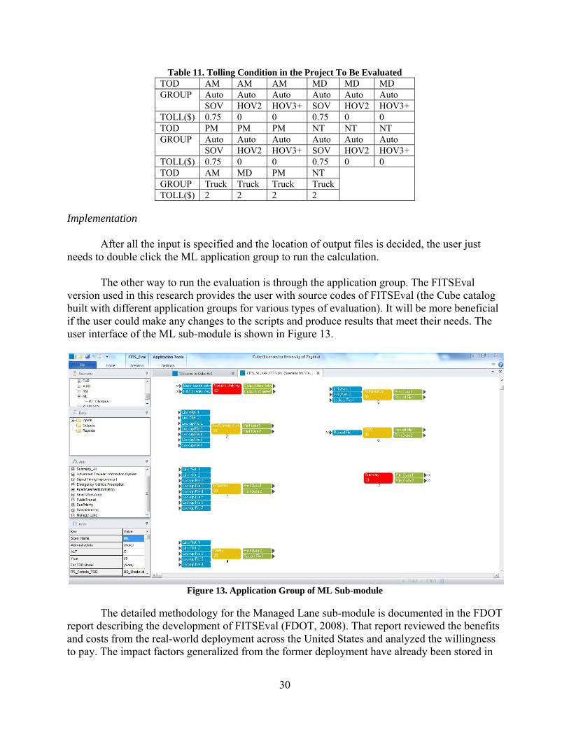
30  

Table 11. Tolling Condition in the Project To Be Evaluated TOD AM AM AM MD MD MD GROUP Auto Auto Auto Auto Auto Auto

SOV HOV2 HOV3+ SOV HOV2 HOV3+ TOLL($) 0.75 0 0 0.75 0 0 TOD PM PM PM NT NT NT GROUP Auto Auto Auto Auto Auto Auto

SOV HOV2 HOV3+ SOV HOV2 HOV3+ TOLL($) 0.75 0 0 0.75 0 0 TOD AM MD PM NT GROUP Truck Truck Truck Truck TOLL($) 2 2 2 2

Implementation

After all the input is specified and the location of output files is decided, the user just needs to double click the ML application group to run the calculation.

The other way to run the evaluation is through the application group. The FITSEval

version used in this research provides the user with source codes of FITSEval (the Cube catalog built with different application groups for various types of evaluation). It will be more beneficial if the user could make any changes to the scripts and produce results that meet their needs. The user interface of the ML sub-module is shown in Figure 13.

Figure 13. Application Group of ML Sub-module

The detailed methodology for the Managed Lane sub-module is documented in the FDOT

report describing the development of FITSEval (FDOT, 2008). That report reviewed the benefits and costs from the real-world deployment across the United States and analyzed the willingness to pay. The impact factors generalized from the former deployment have already been stored in

 

31  

FITSEval, such as the willingness to pay look-up table in terms of the time savings (min/mile). The report also suggested the re-estimation of the network flow changes caused by the ML deployment and the use of the impact factors to estimate the impact of the managed lane deployment.

Two TXT files will be produced by FITSEval: A performance summary and a

benefit/cost summary. The performance summary details the performance in terms of vehicle hours of delay, safety, energy consumption, emissions and road ranger with and without ML deployment. The benefit/cost summary calculates the benefits and costs from different aspects and also gives a benefit cost ratio for comparison with other alternative projects. The Performance summary obtained from Hampton Roads case study is shown in Figure 14.

Figure 14. Performance Summary Obtained From Hampton Roads Case Study

The above network performance comparison is not sufficient because one HOT lane’s

effect on the entire network is trivial and it makes the performance before and after deployment quite similar. Therefore, the script is modified in the Performance (5) application group (see Figure 12) to evaluate the link traffic performance before and after deployment. The first column “w/o-GP” indicates all links considered in the corridor, including links that are to be converted to the HOT lanes. “w-GP” represents the original general purposes links not converted to HOT while “w-HOT” is the original general purpose links that are converted to HOT. The performance of the corridor and alternative are evaluated in terms of VMT, VHT, travel time and congested speed for each of the time periods, as shown in Figure 15. This shows that there is a significant performance improvement with the HOT lane. A similar evaluation can be carried out for the safety, energy consumption and emission evaluation as well. In general the evaluation should be sufficiently robust to show a multidimensional array of performance measures to indicate appropriate differences among alternatives.

 

32  

Figure 15. Corridor-Based Performance With and Without HOT Lane

SUMMARY

The combination of the Cube and FITSEval tools provides planners with a useful analysis capability for conducting studies of operational strategy deployment alternatives. Travel demand models based on Cube are used to provide both the base case loaded network and operational strategy loaded network. The methodologies defined in FITSEval differ from one sub-module to another. What they do is post-process the output of travel demand models and calculate the benefits and costs of deployment based on the embedded algorithm. Figure 16 shows an integrated flow chart for using Cube with FITSEval and illustrates the role of an interface between these models.

CONCLUSIONS

The interface between Cube based travel demand models and FITSEval described in this document is based on the real-world analysis of potential incident management systems and managed lane deployment in Hampton Roads area. This case study effort results in several conclusions, including:

The two models can be successfully integrated to provide a valuable tool for analyzing operational strategy deployments at the planning or macroscopic level. FITSEval is designed to post-process travel demand model outputs from FSUTMS (Cube based) of FDOT. Since VDOT uses Cube as well, FITSEval can be integrated into their planning projects. The integration process requires some level of manual

 

33  

 Figure 16. Methodology Recommendation for Integrating Cube With FITSEval

interfacing, as described in Figure 16, including analysis period definition, facility and area type coding, link period capacity, the volume delay function and operational strategies coding. Some evaluation also requires the development of a methodology to re-estimate network flow conditions resulting from operational strategy deployment. One methodology for evaluating HOT lanes is proposed in this case study and can be used in similar modeling efforts. Many parameters are pre-specified in FITSEval for the convenience of use and they are applicable for most of the cases.

Time-of-day modeling may be helpful when evaluating operational strategies. The

results in Figure 15 show a meaningful difference for some, but not all, of the morning and evening corridor impacts: although speed and travel time changes were similar, there were meaningful differences in the corridor VMT and the corridor VHT.

 

34  

To the extent that agreement between observed and assigned peak period volumes indicates a satisfactory peak period trip distribution matrix, the NHTS data are sufficient for developing a peak period trip distribution matrix. In this study, the obtained time-of-day factors yielded a desired RMSE between assigned volumes and actual volumes. Link-based methods using traffic counts of continuous count stations are also sufficient for evaluating strategies causing limited flow pattern changes.

The post-processing tools such as FITSEval are suitable to be applied to the planning

level operational strategy analysis at the corridor, subarea, and regionwide level. The budget may range from medium/high ($5,000 to $50,000) and the project may last 2 months to 1 year. The staff responsible for the analysis should have experience using travel demand models.

RECOMMENDATIONS

As shown in the two Hampton Roads case studies, the Cube-based travel demand models can be successfully interfaced to conduct impact analysis and alternative screening of potential operational strategy deployments. Recommendations from this work include the following:

1. VDOT’s Transportation Mobility Planning Division in collaboration with

VDOT’s Operations Division should begin to apply FITSEval as a part of their travel demand modeling in regions where operational strategies are under consideration. A pilot test in a volunteer district would provide valuable experience prior to wider implementation.

2. In conjunction with the pilot test, the Virginia Center for Transportation

Innovation and Research (VCTIR) should collect available, existing data on local values for the parameters used in FITSEval.

3. VCTIR should work with the Florida Department of Transportation to exchange

information on needed and developed enhancements to FITSEval as use of the model continues and expands.

BENEFITS AND IMPLEMENTATION PROSPECTS

The methods described in this report will allow operational improvements to be considered alongside traditional capacity improvement in the long range planning process. In many cases, implementation of an operational strategy can delay or alleviate the need for additional lanes and since operational improvements are often, if not always, less expensive than capacity enhancements, significant savings could accrue to VDOT. For example, in the HOT lane case study, the results indicate a delay reduction of 41.5% for the general purpose lane by introducing the HOT lane. The BPR volume-delay function indicates that a 50% increase in physical capacity would be required to achieve similar delay reductions. The construction costs

 

35  

can be as high as $3 million to $6 million per lane-mile, much higher than converting the current lanes to the HOT lanes.

Implementation of the recommendations resulting from this research will require training

and outreach to transportation planners, both within VDOT and at the MPOs around the state.

REFERENCES

Booz-Allen & Hamilton Inc. California Life-Cycle Benefit/Cost Analysis Model (Cal-B/C): User’s Guide. California Department of Transportation, September 1999a.

California Life-Cycle Benefit/Cost Analysis Model (Cal-B/C)—Technical Supplement to User’s

Guide. California Department of Transportation, September 1999b. Cambridge Systematics, Inc. Time-of-Day Modeling Procedures: State-of-the-Practice, State-of-

the-Art. Federal Highway Administration, Washington, DC, 1997. http://tmip.fhwa.dot.gov/resources/clearinghouse/docs/time-day/. Accessed October 1, 2011.

Chen, J.Y. Personal communication, March 22, 2011. Federal Highway Administration. Operations Benefit/Cost Analysis Desk Reference. May 2012. Florida Intelligent Transportation. Systems Evaluation (FITSEVAL) Tools, Final Report, July

2012. Florida Department of Transportation. Evaluation Tools to Support ITS Planning Process:

Development of a Sketch Planning Tool in FSUTMS/Cube Environment. December 15, 2008.

Freund, R.J., and Wilson, W.J. Statistical Methods: Revised Edition. Academic Press, Inc., San

Diego, CA, 1997. FSUTMS /IDAS Interface, Manual Approach, Prepared for FDOT by Cambridge Systematics,

Tallahassee, FL, April 2003. Hadi, M.A., D. Quigley, P. Sinha, and L. Hsia. Benefit and Cost Parameters for Use in

Evaluations by the Intelligent Transportation Systems Deployment Analysis System in Florida, Transportation Research Record, Washington, DC, January 2005.

Hadi, M.A., D. Quigley, P. Sinha, and A. Krishnamurthy. Intelligent Transportation Systems

Deployment Analysis System Customization, Final Report. Prepared for the FDOT by PBSJ, Inc., Tallahassee, FL, October 27, 2005.

 

36  

Heither, C., and M. Thomas. Testing of IDAS Capabilities Using Northeastern Illinois ITS Deployments, Working Paper 03-06. August 2003.

Hogg, R.V., and Ledolter, J. Applied Statistics for Engineers and Physical Scientists, 2nd ed.

Macmillan Publishing Company, New York, 1992. ITS Deployment Analysis System (IDAS) User’s Manual. Prepared for the Federal Highway

Administration by Cambridge Systematics, Oakland, CA, November 2001. Lee J. Personal communication March 27, 2011. Miller, J.S. Email to Jiaqi Ma, March 15, 2011. Miller, J.S. A Model to Forecast Peak Spreading. VTRC 10-R22. Virginia Transportation

Research Council, Charlottesville, 2012. http://www.virginiadot.org/vtrc/main/online_reports/pdf/12-r11.pdf. Accessed September 5, 2012.

Montgomery, D.C. Introduction to Statistical Quality Control, 4th ed. John Wiley & Sons, Inc.,

New York, 2001a. PB Farradyne Inc. Hampton Roads Intelligent Transportation Systems Strategic Plan, Final

Report. Prepared for the Virginia Department of Transportation Hampton Roads Planning District Commission, April 2004.

Pendyala, R.M. Time of Day Modeling Procedures for Implementation in FSUTMS. Final

Report, BC353-08. Prepared for the FDOT by University of South Florida, December 2002.

Science Applications International Corporation. User’s Manual for SCRITS, Screening Analysis

for ITS. Prepared for Federal Highway Administration Office of Traffic Management and ITS Applications, 1999.

The 2005 Update of Florida’s ITS Strategic Plan, Final Report. Prepared by FDOT ITS

Division, Tallahassee, FL, December 2, 2005. Thill, J.C., and G. Rogova. The ITS Options Analysis Model Technical Documentation.

Produced for the New York DOT by Calspan UB Research Center and University at Buffalo, Buffalo, NY, October 13, 2005.

Tri-County Regional Planning Commission. Regional 2035 Transportation Plan, 2010.

http://www.tri-co.org/trp.htm#. User’s Manual for SCRITS, Screening Analysis for ITS. Prepared for the Federal Highway

Administration Office of Traffic Management and ITS Applications. Prepared by Science Applications International Corporation, January 1999.

 

37  

Virginia Department of Transportation. Hampton Roads Model Methodology Report (Draft V0.16). January 2012.

Virginia Department of Transportation. Hampton Roads Model User’s Guide (Draft V0.06).

January 2012. Virginia Department of Transportation. VDOT Traffic Engineering, undated.

http://tedweb/tms/jsp/. Accessed January 15, 2012. Zhou, X., Mahmassani, H.S. and Zhang K. Dynamic Micro-assignment Modeling Approach for

Integrated Multimodal Urban Corridor Management. Transportation Research Part C16, 2008, pp. 167-186.

 

38  

 

39  

APPENDIX A

CUBE SCRIPTS FOR NETWORK INPUT PREPARATION

The scripts provided here are for the network preparation with ML deployed. These codes should be in compatible with the corresponding variable name replacement file. The user can refer to it for other network preparation in this research.  UN PGM=NETWORK FILEO NETO = "{CATALOG_DIR}\Network_ML\HR_TOD_MLITS.NET" FILEI LINKI[4] = "{CATALOG_DIR}\Network_ML\Nt_OP_FDBKNET.NET" FILEI LINKI[3] = "{CATALOG_DIR}\Network_ML\Md_OP_FDBKNET.NET" FILEI LINKI[2] = "{CATALOG_DIR}\Network_ML\PM_PK_FDBKNET.NET" FILEI LINKI[1] = "{CATALOG_DIR}\Network_ML\AM_PK_FDBKNET.NET"  PROCESS  PHASE=LINKMERGE   ; Use this phase to make computations and selections of any data on the LINKI files.         AM_FFLOWSPEED=LI.1.FFLOWSPEED         PM_FFLOWSPEED=LI.2.FFLOWSPEED         Md_FFLOWSPEED=LI.3.FFLOWSPEED         Nt_FFLOWSPEED=LI.4.FFLOWSPEED         OP_FFLOWSPEED=LI.4.FFLOWSPEED         AD_FFLOWSPEED=LI.4.FFLOWSPEED                  AM_FFTIME=LI.1.FFTIME         PM_FFTIME=LI.2.FFTIME         Md_FFTIME=LI.3.FFTIME         Nt_FFTIME=LI.4.FFTIME         OP_FFTIME=LI.4.FFTIME         AD_FFTIME=LI.4.FFTIME                  AM_FDBKTIME=LI.1.FDBKTIME         PM_FDBKTIME=LI.2.FDBKTIME         Md_FDBKTIME=LI.3.FDBKTIME         Nt_FDBKTIME=LI.4.FDBKTIME                  AM_FDBKVOL=LI.1.FDBKVOL         PM_FDBKVOL=LI.2.FDBKVOL         Md_FDBKVOL=LI.3.FDBKVOL         Nt_FDBKVOL=LI.4.FDBKVOL                  AM_LINK_CAP=LI.1.LINK_CAP*LI.1.LANES*2.6         PM_LINK_CAP=LI.2.LINK_CAP*LI.2.LANES*2.9         Md_LINK_CAP=LI.3.LINK_CAP*LI.3.LANES*5.0         Nt_LINK_CAP=LI.4.LINK_CAP*LI.4.LANES*4.3         OP_LINK_CAP=Md_LINK_CAP+Nt_LINK_CAP         AD_LINK_CAP=AM_LINK_CAP+PM_LINK_CAP+Md_LINK_CAP+Nt_LINK_CAP          

 

40  

        AM_TV=li.1.V_1         PM_TV=li.2.V_1         Md_TV=li.3.V_1         Nt_TV=li.4.V_1         OP_TV=li.3.V_1+li.4.V_1         AD_TV=AM_TV+MD_TV+PM_TV+NT_TV                  CGSTD_TIME_AM=LI.1.TIME_1         CGSTD_TIME_PM=LI.2.TIME_1         CGSTD_TIME_MD=LI.3.TIME_1         CGSTD_TIME_NT=LI.4.TIME_1         CGSTD_TIME_OP=(LI.3.TIME_1+LI.4.TIME_1)/2         CGSTD_TIME_AD=(LI.1.TIME_1+LI.2.TIME_1+LI.3.TIME_1+LI.4.TIME_1)/4                 VOLCAP_AM=LI.1.VC_1         VOLCAP_pM=LI.2.VC_1         VOLCAP_MD=LI.3.VC_1         VOLCAP_NT=LI.4.VC_1         VOLCAP_OP=OP_TV/OP_LINK_CAP         VOLCAP_AD=AD_TV/AD_LINK_CAP                  CGSTD_SPEED_AM=LI.1.CSPD_1         CGSTD_SPEED_PM=LI.2.CSPD_1         CGSTD_SPEED_MD=LI.3.CSPD_1         CGSTD_SPEED_NT=LI.4.CSPD_1         CGSTD_SPEED_OP= LI.3.DISTANCE*60/CGSTD_TIME_OP         CGSTD_SPEED_AD= LI.3.DISTANCE*60/CGSTD_TIME_AD                  AM_VMT=LI.1.VDT_1         PM_VMT=LI.2.VDT_1         Md_VMT=LI.3.VDT_1         Nt_VMT=LI.4.VDT_1         OP_VMT=Md_VMT+Nt_VMT         AD_VMT=AM_VMT+MD_VMT+PM_VMT+NT_VMT                  AM_VHT=LI.1.VHT_1         PM_VHT=LI.2.VHT_1         Md_VHT=LI.3.VHT_1         Nt_VHT=LI.4.VHT_1         OP_VHT=Md_VHT+Nt_VHT         AD_VHT=AM_VHT+MD_VHT+PM_VHT+NT_VHT            DRV_ALONE_AM= round(li.1.V1_1+li.1.V2_1+li.1.V3_1+li.1.V4_1+li.1.V5_1)   DRV_ALONE_PM= round(li.2.V1_1+li.2.V2_1+li.2.V3_1+li.2.V4_1+li.2.V5_1)   DRV_ALONE_MD= round(li.3.V1_1+li.3.V2_1+li.3.V3_1+li.3.V4_1+li.3.V5_1)   DRV_ALONE_NT= round(li.4.V1_1+li.4.V2_1+li.4.V3_1+li.4.V4_1+li.4.V5_1)   DRV_ALONE_OP= DRV_ALONE_MD + DRV_ALONE_NT   DRV_ALONE_24= DRV_ALONE_AM + DRV_ALONE_PM + DRV_ALONE_MD + DRV_ALONE_NT 

 

41  

  CARPOOL_AM= round(li.1.V6_1+li.1.V7_1+li.1.V8_1+li.1.V9_1+li.1.V10_1)   CARPOOL_PM= round(li.2.V6_1+li.2.V7_1+li.2.V8_1+li.2.V9_1+li.2.V10_1)   CARPOOL_MD= round(li.3.V6_1+li.3.V7_1+li.3.V8_1+li.3.V9_1+li.3.V10_1)   CARPOOL_NT= round(li.4.V6_1+li.4.V7_1+li.4.V8_1+li.4.V9_1+li.4.V10_1)   CARPOOL_OP= CARPOOL_MD + CARPOOL_NT   CARPOOL_24= CARPOOL_MD + CARPOOL_NT + CARPOOL_MD + CARPOOL_NT      CARPOOL1_AM= round(li.1.V11_1+li.1.V12_1+li.1.V13_1+li.1.V14_1+li.1.V15_1)   CARPOOL1_PM= round(li.2.V11_1+li.2.V12_1+li.2.V13_1+li.2.V14_1+li.2.V15_1)   CARPOOL1_MD= round(li.3.V11_1+li.3.V12_1+li.3.V13_1+li.3.V14_1+li.3.V15_1)   CARPOOL1_NT= round(li.4.V11_1+li.4.V12_1+li.4.V13_1+li.4.V14_1+li.4.V15_1)   CARPOOL1_OP= CARPOOL_MD + CARPOOL_NT   CARPOOL1_24= CARPOOL_MD + CARPOOL_NT + CARPOOL_MD + CARPOOL_NT        TRUCK_TAXI_AM= round(li.1.V16_1+li.1.V17_1+li.1.V18_1+li.1.V19_1+li.1.V20_1)   TRUCK_TAXI_PM= round(li.2.V16_1+li.2.V17_1+li.2.V18_1+li.2.V19_1+li.2.V20_1)   TRUCK_TAXI_MD= round(li.3.V16_1+li.3.V17_1+li.3.V18_1+li.3.V19_1+li.3.V20_1)   TRUCK_TAXI_NT= round(li.4.V16_1+li.4.V17_1+li.4.V18_1+li.4.V19_1+li.4.V20_1)   TRUCK_TAXI_OP= TRUCK_TAXI_MD + TRUCK_TAXI_NT   TRUCK_TAXI_24= TRUCK_TAXI_AM + TRUCK_TAXI_PM + TRUCK_TAXI_OP      CONFAC_AM=0.3846   CONFAC_PM=0.3448   CONFAC_MD=0.2   CONFAC_NT=0.2325   CONFAC_OP=0.1075   CONFAC_24H=0.1      BPRCOEFFICIENT= 0.15   BPREXPONENT= 4        if (Li.1.AREATYPE='1')        AREATYPE3=STR(1,1,0)     elseif  (Li.1.AREATYPE='2')        AREATYPE3=STR(2,1,0)     elseif  (Li.1.AREATYPE='3')        AREATYPE3=STR(3,1,0)     elseif  (Li.1.AREATYPE='4')        AREATYPE3=STR(4,1,0)     else        AREATYPE3=STR(5,1,0)  ENDIF        if (Li.1.AREATYPE='1','2')        ATYPE=11     elseif  (Li.1.AREATYPE='3')        ATYPE=41     else 

 

42  

       ATYPE=51     endif      if (Li.1.FACTYPE='1','2')        FTYPE=11     elseif  (Li.1.FACTYPE='3','4')        FTYPE=21     elseif  (Li.1.FACTYPE='5')        FTYPE=31     elseif  (Li.1.FACTYPE='6','7','8')        FTYPE=41     elseif  (Li.1.FACTYPE='9','10')        FTYPE=71     elseif  (Li.1.FACTYPE='11','12')        FTYPE=51     ENDIF          IF (Li.1.TOLL_GRP!=0)         HOT=1         FTYPE=82         CORR=14     ELSE         HOT=0         CORR=0     ENDIF          IF (VAL(LI.1.HOVTYPE) <> 0 && LI.1.TOLL_GRP = 0)   HOT=2,FTYPE=86 HOT=0         ENDPROCESS ENDRUN 

 

43  

APPENDIX B

DEFINITION OF FACILITY TYPE AND AREA TYPE IN FSUTMS AND FITSEval

There are two definitions of facility type in FITSEval, two-digit (from 10 to 99) and one-digit (from 1 to 9). The one-digit definition is shown below. The two-digit definition is an expansion for the one-digit definition. The example of freeway can be shown below. More detailed two-digit definition can be found on the FSUTMS modeling guide book.

Table B1. One-digit Facility Type in FSUTMS and FITSEval Code Facility Type

1 Freeway 2 Divided Arterial 3 Undivided Arterial 4 Collector 5 Centroid Connector 6 One-Way 7 Not Used 8 HOV Links 9 Toll Links

Table B2. Demonstration of Two-Digit Facility Type in FSUTMS and FITSEval

1x Freeways Expressways(FT 10 is default) 11 Urban Freeway Group 1 (cities of 500,000 or more) 12 Other Freeway (not in Group 1) 15 Collector/Distributor Lane 16 Controlled Access Expressway 17 Controlled Access Parkway

Table B3. Area Type Description in FSUTMS and FITSEval

1x CBD Areas (AT 10 is default) 11 Urbanized Area (over 500,000) Primary City Central Business District 12 Urbanized Area (under 500,000) Primary City Central Business District 13 Other Urbanized Area Central Business District and Small City 14 Non-Urbanized Area Small City Downtown

2x CBD Fringe Areas (AT 20 is default) 21 All Central Business District (CBD) Fringe Areas

3x Residential Areas (AT 30 is default) 31 Residential Area of Urbanized Areas 32 Undeveloped Portions of Urbanized Areas 33 Transitioning Areas/Urban Areas over 5,000 Population 34 Beach Residential (per SERPM)

4x OBD Areas (AT 40 is default) 41 High Density Outlying Business District 42 Other Outlying Business District 43 Beach OBD (per SERPM)

5x Rural Areas (AT 50 is default) 51 Developed Rural Areas/Small Cities under 5,000 Population 52 Undeveloped Rural Areas

 

44  

 

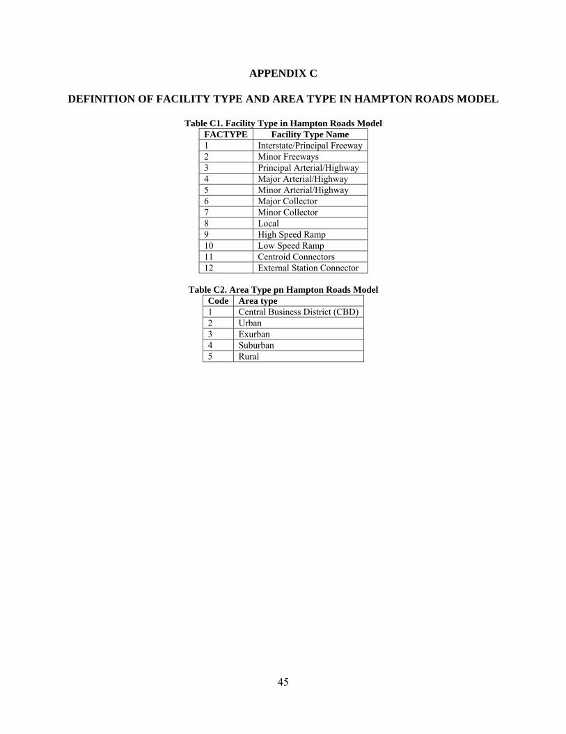
45  

APPENDIX C

DEFINITION OF FACILITY TYPE AND AREA TYPE IN HAMPTON ROADS MODEL

Table C1. Facility Type in Hampton Roads Model FACTYPE Facility Type Name 1 Interstate/Principal Freeway 2 Minor Freeways 3 Principal Arterial/Highway 4 Major Arterial/Highway 5 Minor Arterial/Highway 6 Major Collector 7 Minor Collector 8 Local 9 High Speed Ramp 10 Low Speed Ramp 11 Centroid Connectors 12 External Station Connector

Table C2. Area Type pn Hampton Roads Model

Code Area type 1 Central Business District (CBD) 2 Urban 3 Exurban 4 Suburban 5 Rural

 

46  

 

47  

APPENDIX D

VARIABLE REPLACEMENT CSV FILE FOR IM EVALUATION IN HAMPTON ROADS MODEL (AM PEAK)

Three such files for AM peak, PM peak and Off-peak variable replacement should be

input by the user.

Table D1. Variable Replacement File for IM Sub-module Application (AM Peak Period) AM_ToTVol li AM_V_1 ; AM total volume AM_DAVOL li DRV_ALONE_AM ; AM drive alone volume AM_SRVOL li CARPOOL_AM ; AM carpool volume AM_TRKVOL li TRUCKAM ; AM truck volume CAPACITY li AM_LINK_CAP ; Link capacity (LOS E) LOSCCAP li AM_LINK_CAP ; Capacity under LOS C AM_VCLOSC li AM_VC_1 ; AM V/C ratio under LOS C capacity AM_CONGTIME li AM_TIME_1 ; AM link congested travel time AM_CONGSPD li AM_CSPD_1 ; AM link congested speed AM_VMT li AM_VDT_1 ; AM Vehicle mile traveled AM_VHT li AM_VHT_1 ; AM vehicle hour traveled AT2_OLD li AREATYPE2 ; Link area type code (2 digits) FTC2 li FACTYPE2 ; Link facility type code 1-12) Time li AM_FFTIME ; Daily link free flow speed Distance li DISTANCE ; Link distance (miles) BPRCOEFFICIENT li BPRCOEFFICIENT ; BPR equation parameter a BPREXPONENT li BPREXPONENT ; BPR equation parameter b FREEFLOWSPEED li AM_FFLOWSPEED ; Link free flow speed CONFACAMP li CONFAC_AM ; AM CONF factor Num_Lanes li LANES ; link number of lanes

 

48  

 

49  

APPENDIX E

VARIABLE REPLACEMENT CSV FILE FOR ML EVALUATION IN HAMPTON ROADS MODEL

Two such files for the base network and Managed Lane deployment network variable

replacement should be input by the user.

Table E1. Variable Replacement File for ML Sub-module Application Distance li Distance ; AM period link distance CORTYPE li CORR ; Link corridor type code FTC2 li FTYPE ; Link facility type code (with two digits) Area_Type li ATYPE ; Link area type code (with two digits) HOT li HOT ; Link HOT flag (0,1) AM_DAVOL li DRV_ALONE_AM ; AM period drive alone volume AM_SR2VOL li CARPOOL_AM ; AM period vehicle volume with 2 passenger AM_SR3VOL li CARPOOL1_AM ; AM period vehicle volume with 3+ passenger AM_TRKVOL li TRUCK_TAXI_AM ; AM period Truck volume AM_TOTVOL li AM_TV ;AM period total volume AM_CONGSPD li CGSTD_SPEED_AM ; AM period link congested speed AM_CONGTIME li CGSTD_TIME_AM ; AM period link congested travel time AM_VMT li AM_VMT ; AM period link vehicle mile traveled AM_VHT li AM_VHT ; AM period link vehicle hour traveled AM_VCLOSC li VOLCAP_AM ; AM period link capacity V/C ratio based on LOS C capcity PM_DAVOL li DRV_ALONE_PM ; PM period drive alone volume PM_SR2VOL li CARPOOL_PM ; PM period vehicle volume with 2 passenger PM_SR3VOL li CARPOOL1_PM ; PM period vehicle volume with 3+ passenger PM_TRKVOL li TRUCK_TAXI_PM ; PM period Truck volume PM_TOTVOL li PM_TV ;PM period total volume PM_CONGSPD li CGSTD_SPEED_PM ; PM period link congested speed PM_CONGTIME li CGSTD_TIME_PM ; PM period link congested travel time PM_VMT li PM_VMT ; PM period link vehicle mile traveled PM_VHT li PM_VHT ; PM period link vehicle hour traveled PM_VCLOSC li VOLCAP_PM ; PM period link capacity V/C ratio based on LOS C capcity OF_DAVOL li DRV_ALONE_OP ; OP period drive alone volume OF_SR2VOL li CARPOOL_OP ; OP period vehicle volume with 2 passenger OF_SR3VOL li CARPOOL1_OP ; OP period vehicle volume with 3+ passenger OF_TRKVOL li TRUCK_TAXI_OP ; OP period Truck volume OF_TOTVOL li OP_TV ;Off peak period total volume OF_CONGSPD li CGSTD_SPEED_OP ; OP period link congested speed OF_CONGTIME li CGSTD_TIME_OP ; OP period link congested travel time OF_VMT li OP_VMT ; OP period link vehicle mile traveled OF_VHT li OP_VHT ; OP period link vehicle hour traveled OF_VCLOSC li VOLCAP_OP ; OP period link capacity V/C ratio based on LOS C capcity

 

50  

 

51  

APPENDIX F

HOT LANE MODELING SCRIPTS FOR CUBE VOYAGER

The following scripts are based on the 2009 Hampton Roads travel demand model application procedure and are used in the HOT case study deployment in this report. The modelers can make use of the modeling and scripting if the same methodology is adopted. RUN PGM=HIGHWAY PRNFILE="{CATALOG_DIR}\OUTPUT\{Scenario_FullName}\LOGS\HAHWY00B.PRN" MSG='Highway Assignment' FILEI TURNPENI = "{Turn Penalties}" FILEI NETI = "{CATALOG_DIR}\OUTPUT\{Scenario_FullName}\AM_Feedback_Network.NET" FILEI MATI[1] = "{CATALOG_DIR}\OUTPUT\{SCENARIO_FULLNAME}\AM_Pk_Final_TripTable_VOT_TMP.DAT" FILEO NETO = "{CATALOG_DIR}\OUTPUT\{SCENARIO_FULLNAME}\AM_Pk_LOADED_{Alternative}.NET"      ; Enable a single extra node in Cube Cluster     DISTRIBUTEINTRASTEP PROCESSID='HRD' PROCESSLIST={PROCESSLIST} COMMPATH='{Catalog_Dir}\cluster'          PARAMETERS,         ZONES={Total Zones},         MAXITERS={Hwy_Iterations},         COMBINE=EQUI,         RELATIVEGAP=0.010          ; These two are period specific         PRD = 'AM'         CAPFAC = {AM CAPFAC}      ; Assign VOTS by Bucket through Key or flat file      BASEVOT = {BaseVOT}                 ; 2009 cents/min (Taken from Florida model $10/hr)      VOT_1 = BaseVOT * 0.5           ; Lowest Value of time    units??      VOT_2 = BaseVOT * 0.8           ; low mid VOT             5.95      VOT_3 = BaseVOT * 1.0           ; mid VOT                 7.43      VOT_4 = BaseVOT * 1.2           ; high mid VOT            8.92      VOT_5 = BaseVOT * 1.5           ; highest VOT            11.15           READ FILE = "{TOLL}"              ;Conical equations have one parameter alpha, beta is function of alpha, modelers can make use of the VDF consistent with their own travel demand models     Alpha2=9.0     Beta2= (2.0*Alpha2‐1)/(2.0*Alpha2‐2)     Alpha3=7.0     Beta3= (2.0*Alpha3‐1)/(2.0*Alpha3‐2)     Alpha4=4.5     Beta4= (2.0*Alpha4‐1)/(2.0*Alpha4‐2) 

 

52  

    Alpha5=2.0     Beta5= (2.0*Alpha5‐1)/(2.0*Alpha5‐2)          FUNCTION {         V = VOL[1]  + VOL[2]  + VOL[3]  + VOL[4]  + VOL[5]  +       ; SOV             VOL[6]  + VOL[7]  + VOL[8]  + VOL[9]  + VOL[10] +       ; HOV2+             VOL[11] + VOL[12] + VOL[13] + VOL[14] + VOL[15] +       ; HOV3+             2.0*(VOL[16] + VOL[17] + VOL[18] + VOL[19] + VOL[20])    ; Trucks...converting them to PCE's             ; Conical VDF equations              TC[1] = T0             TC[2] = T0 * (2 + SQRT(Alpha2^2 * (1‐VC)^2 + Beta2^2) ‐ Alpha2 * (1‐VC) ‐ Beta2)             TC[3] = T0 * (2 + SQRT(Alpha3^2 * (1‐VC)^2 + Beta3^2) ‐ Alpha3 * (1‐VC) ‐ Beta3)             TC[4] = T0 * (2 + SQRT(Alpha4^2 * (1‐VC)^2 + Beta4^2) ‐ Alpha4 * (1‐VC) ‐ Beta4)             TC[5] = T0 * (2 + SQRT(Alpha5^2 * (1‐VC)^2 + Beta5^2) ‐ Alpha5 * (1‐VC) ‐ Beta5)         }      PHASE=LINKREAD         ; set the substring position based on period.  AM=1, MD=2, PM=3, NT=4          if (PRD = 'AM')            bb=1          elseif (PRD = 'MD')            bb=2          elseif (PRD = 'PM')            bb=3          elseif (PRD = 'NT')            bb=4          endif           ; Define pathbuilding groups (so HOV facilities can be ignored)         IF (VAL(LI.HOVTYPE) = 0 || VAL(SUBSTR(LI.HOVTYPE,bb,1)) =1) ADDTOGROUP=1      ; all vehciles allowed         IF (SUBSTR(LI.HOVTYPE,bb,1) = '2' && LI.TOLL_GRP = 0)       ADDTOGROUP=2      ; HOV2+ only         IF (SUBSTR(LI.HOVTYPE,bb,1) = '3' && LI.TOLL_GRP = 0)       ADDTOGROUP=3      ; HOV3+ only         IF (STRPOS('Y',LI.TRK_PHB)+strpos('A',li.trk_phb)>0)         ADDTOGROUP=5      ; Trucks Prohibited         IF (SUBSTR(LI.HOVTYPE,bb,1) = '9')                          ADDTOGROUP=9      ; Closed to all vehicles              C=LI.LINK_CAP*LI.LANES*{AM CAPFAC}         T0=LI.DISTANCE*60/LI.FFLOWSPEED          if (PRD = 'AM')            LW.AMSOVTOLL = (TOLLLU( 1,LI.TOLL_GRP) + (TOLLLU(17,LI.TOLL_GRP) * LI.DISTANCE)) * CONFAC(1,LI.TOLL_GRP)            LW.AMHV2TOLL = (TOLLLU( 2,LI.TOLL_GRP) + (TOLLLU(18,LI.TOLL_GRP) * LI.DISTANCE)) * CONFAC(1,LI.TOLL_GRP)            LW.AMHV3TOLL = (TOLLLU( 3,LI.TOLL_GRP) + (TOLLLU(19,LI.TOLL_GRP) * LI.DISTANCE)) * CONFAC(1,LI.TOLL_GRP) 

 

53  

           LW.AMTRKTOLL = (TOLLLU(13,LI.TOLL_GRP) + (TOLLLU(29,LI.TOLL_GRP) * LI.DISTANCE)) * CONFAC(1,LI.TOLL_GRP)            LW.AMGATE    = GATELU( 1,LI.TOLL_GRP)         elseif (PRD = 'MD')            LW.MDSOVTOLL = (TOLLLU( 4,LI.TOLL_GRP) + (TOLLLU(20,LI.TOLL_GRP) * LI.DISTANCE)) * CONFAC(1,LI.TOLL_GRP)            LW.MDHV2TOLL = (TOLLLU( 5,LI.TOLL_GRP) + (TOLLLU(21,LI.TOLL_GRP) * LI.DISTANCE)) * CONFAC(1,LI.TOLL_GRP)            LW.MDHV3TOLL = (TOLLLU( 6,LI.TOLL_GRP) + (TOLLLU(22,LI.TOLL_GRP) * LI.DISTANCE)) * CONFAC(1,LI.TOLL_GRP)            LW.MDTRKTOLL = (TOLLLU(14,LI.TOLL_GRP) + (TOLLLU(30,LI.TOLL_GRP) * LI.DISTANCE)) * CONFAC(1,LI.TOLL_GRP)            LW.MDGATE    = GATELU( 2,LI.TOLL_GRP)         elseif (PRD = 'PM')            LW.PMSOVTOLL = (TOLLLU( 7,LI.TOLL_GRP) + (TOLLLU(23,LI.TOLL_GRP) * LI.DISTANCE)) * CONFAC(1,LI.TOLL_GRP)            LW.PMHV2TOLL = (TOLLLU( 8,LI.TOLL_GRP) + (TOLLLU(24,LI.TOLL_GRP) * LI.DISTANCE)) * CONFAC(1,LI.TOLL_GRP)            LW.PMHV3TOLL = (TOLLLU( 9,LI.TOLL_GRP) + (TOLLLU(25,LI.TOLL_GRP) * LI.DISTANCE)) * CONFAC(1,LI.TOLL_GRP)            LW.PMTRKTOLL = (TOLLLU(15,LI.TOLL_GRP) + (TOLLLU(31,LI.TOLL_GRP) * LI.DISTANCE)) * CONFAC(1,LI.TOLL_GRP)            LW.PMGATE    = GATELU( 3,LI.TOLL_GRP)         elseif (PRD = 'NT')            LW.NTSOVTOLL = (TOLLLU(10,LI.TOLL_GRP) + (TOLLLU(26,LI.TOLL_GRP) * LI.DISTANCE)) * CONFAC(1,LI.TOLL_GRP)            LW.NTHV2TOLL = (TOLLLU(11,LI.TOLL_GRP) + (TOLLLU(27,LI.TOLL_GRP) * LI.DISTANCE)) * CONFAC(1,LI.TOLL_GRP)            LW.NTHV3TOLL = (TOLLLU(12,LI.TOLL_GRP) + (TOLLLU(28,LI.TOLL_GRP) * LI.DISTANCE)) * CONFAC(1,LI.TOLL_GRP)            LW.NTTRKTOLL = (TOLLLU(16,LI.TOLL_GRP) + (TOLLLU(32,LI.TOLL_GRP) * LI.DISTANCE)) * CONFAC(1,LI.TOLL_GRP)            LW.NTGATE    = GATELU( 4,LI.TOLL_GRP)         endif            ;Define generalized cost as a function of time, distance, and toll in year 2009 US cents        ;SOV Vehicles         LW.COST_SOV_GRP1=(T0) + (LW.AMSOVTOLL/VOT_1) + LW.AMGATE         LW.COST_SOV_GRP2=(T0) + (LW.AMSOVTOLL/VOT_2) + LW.AMGATE         LW.COST_SOV_GRP3=(T0) + (LW.AMSOVTOLL/VOT_3) + LW.AMGATE         LW.COST_SOV_GRP4=(T0) + (LW.AMSOVTOLL/VOT_4) + LW.AMGATE         LW.COST_SOV_GRP5=(T0) + (LW.AMSOVTOLL/VOT_5) + LW.AMGATE         ;HOV2+ Vehicles         LW.COST_HV2_GRP1=(T0) + (LW.AMHV2TOLL/VOT_1) + LW.AMGATE         LW.COST_HV2_GRP2=(T0) + (LW.AMHV2TOLL/VOT_2) + LW.AMGATE         LW.COST_HV2_GRP3=(T0) + (LW.AMHV2TOLL/VOT_3) + LW.AMGATE         LW.COST_HV2_GRP4=(T0) + (LW.AMHV2TOLL/VOT_4) + LW.AMGATE 

 

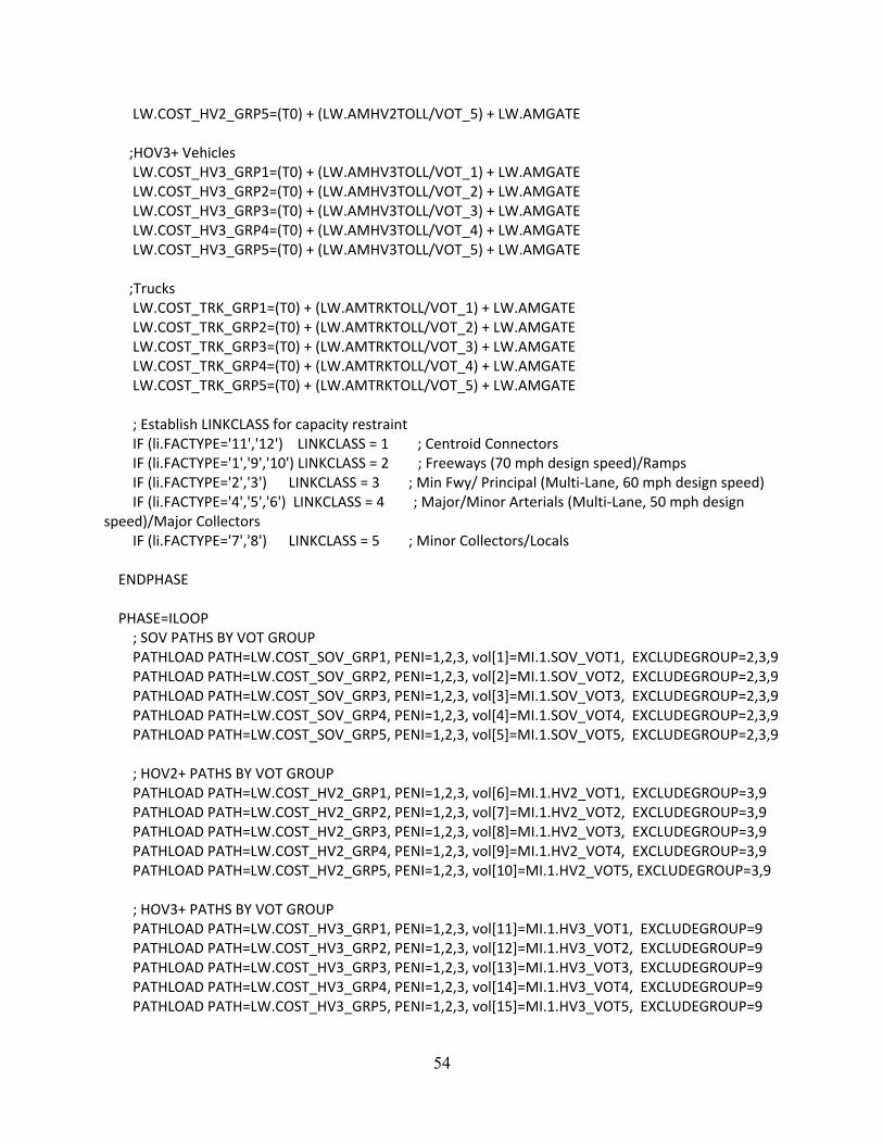
54  

        LW.COST_HV2_GRP5=(T0) + (LW.AMHV2TOLL/VOT_5) + LW.AMGATE         ;HOV3+ Vehicles         LW.COST_HV3_GRP1=(T0) + (LW.AMHV3TOLL/VOT_1) + LW.AMGATE         LW.COST_HV3_GRP2=(T0) + (LW.AMHV3TOLL/VOT_2) + LW.AMGATE         LW.COST_HV3_GRP3=(T0) + (LW.AMHV3TOLL/VOT_3) + LW.AMGATE         LW.COST_HV3_GRP4=(T0) + (LW.AMHV3TOLL/VOT_4) + LW.AMGATE         LW.COST_HV3_GRP5=(T0) + (LW.AMHV3TOLL/VOT_5) + LW.AMGATE         ;Trucks         LW.COST_TRK_GRP1=(T0) + (LW.AMTRKTOLL/VOT_1) + LW.AMGATE         LW.COST_TRK_GRP2=(T0) + (LW.AMTRKTOLL/VOT_2) + LW.AMGATE         LW.COST_TRK_GRP3=(T0) + (LW.AMTRKTOLL/VOT_3) + LW.AMGATE         LW.COST_TRK_GRP4=(T0) + (LW.AMTRKTOLL/VOT_4) + LW.AMGATE         LW.COST_TRK_GRP5=(T0) + (LW.AMTRKTOLL/VOT_5) + LW.AMGATE              ; Establish LINKCLASS for capacity restraint         IF (li.FACTYPE='11','12')    LINKCLASS = 1        ; Centroid Connectors         IF (li.FACTYPE='1','9','10') LINKCLASS = 2        ; Freeways (70 mph design speed)/Ramps         IF (li.FACTYPE='2','3')      LINKCLASS = 3        ; Min Fwy/ Principal (Multi‐Lane, 60 mph design speed)         IF (li.FACTYPE='4','5','6')  LINKCLASS = 4        ; Major/Minor Arterials (Multi‐Lane, 50 mph design speed)/Major Collectors         IF (li.FACTYPE='7','8')      LINKCLASS = 5        ; Minor Collectors/Locals          ENDPHASE      PHASE=ILOOP         ; SOV PATHS BY VOT GROUP         PATHLOAD PATH=LW.COST_SOV_GRP1, PENI=1,2,3, vol[1]=MI.1.SOV_VOT1,  EXCLUDEGROUP=2,3,9         PATHLOAD PATH=LW.COST_SOV_GRP2, PENI=1,2,3, vol[2]=MI.1.SOV_VOT2,  EXCLUDEGROUP=2,3,9         PATHLOAD PATH=LW.COST_SOV_GRP3, PENI=1,2,3, vol[3]=MI.1.SOV_VOT3,  EXCLUDEGROUP=2,3,9         PATHLOAD PATH=LW.COST_SOV_GRP4, PENI=1,2,3, vol[4]=MI.1.SOV_VOT4,  EXCLUDEGROUP=2,3,9         PATHLOAD PATH=LW.COST_SOV_GRP5, PENI=1,2,3, vol[5]=MI.1.SOV_VOT5,  EXCLUDEGROUP=2,3,9           ; HOV2+ PATHS BY VOT GROUP         PATHLOAD PATH=LW.COST_HV2_GRP1, PENI=1,2,3, vol[6]=MI.1.HV2_VOT1,  EXCLUDEGROUP=3,9         PATHLOAD PATH=LW.COST_HV2_GRP2, PENI=1,2,3, vol[7]=MI.1.HV2_VOT2,  EXCLUDEGROUP=3,9         PATHLOAD PATH=LW.COST_HV2_GRP3, PENI=1,2,3, vol[8]=MI.1.HV2_VOT3,  EXCLUDEGROUP=3,9         PATHLOAD PATH=LW.COST_HV2_GRP4, PENI=1,2,3, vol[9]=MI.1.HV2_VOT4,  EXCLUDEGROUP=3,9         PATHLOAD PATH=LW.COST_HV2_GRP5, PENI=1,2,3, vol[10]=MI.1.HV2_VOT5, EXCLUDEGROUP=3,9          ; HOV3+ PATHS BY VOT GROUP         PATHLOAD PATH=LW.COST_HV3_GRP1, PENI=1,2,3, vol[11]=MI.1.HV3_VOT1,  EXCLUDEGROUP=9         PATHLOAD PATH=LW.COST_HV3_GRP2, PENI=1,2,3, vol[12]=MI.1.HV3_VOT2,  EXCLUDEGROUP=9         PATHLOAD PATH=LW.COST_HV3_GRP3, PENI=1,2,3, vol[13]=MI.1.HV3_VOT3,  EXCLUDEGROUP=9         PATHLOAD PATH=LW.COST_HV3_GRP4, PENI=1,2,3, vol[14]=MI.1.HV3_VOT4,  EXCLUDEGROUP=9         PATHLOAD PATH=LW.COST_HV3_GRP5, PENI=1,2,3, vol[15]=MI.1.HV3_VOT5,  EXCLUDEGROUP=9  

 

55  

        ; TRUCK PATHS BY VOT GROUP         PATHLOAD PATH=LW.COST_TRK_GRP1, PENI=1,2,3, vol[16]=MI.1.TRK_VOT1,  EXCLUDEGROUP=2,3,5,9         PATHLOAD PATH=LW.COST_TRK_GRP2, PENI=1,2,3, vol[17]=MI.1.TRK_VOT2,  EXCLUDEGROUP=2,3,5,9         PATHLOAD PATH=LW.COST_TRK_GRP3, PENI=1,2,3, vol[18]=MI.1.TRK_VOT3,  EXCLUDEGROUP=2,3,5,9         PATHLOAD PATH=LW.COST_TRK_GRP4, PENI=1,2,3, vol[19]=MI.1.TRK_VOT4,  EXCLUDEGROUP=2,3,5,9         PATHLOAD PATH=LW.COST_TRK_GRP5, PENI=1,2,3, vol[20]=MI.1.TRK_VOT5,  EXCLUDEGROUP=2,3,5,9     ENDPHASE      PHASE=ADJUST         ; Update travel times factors for peak and off‐peak travel conditions         ; Define revised volume‐delay relationships for commuters and non‐commuters                 ; Update generalized cost          ; SOV Vehicles         LW.COST_SOV_GRP1=(TIME) + (LW.AMSOVTOLL/VOT_1) + LW.AMGATE         LW.COST_SOV_GRP2=(TIME) + (LW.AMSOVTOLL/VOT_2) + LW.AMGATE         LW.COST_SOV_GRP3=(TIME) + (LW.AMSOVTOLL/VOT_3) + LW.AMGATE         LW.COST_SOV_GRP4=(TIME) + (LW.AMSOVTOLL/VOT_4) + LW.AMGATE         LW.COST_SOV_GRP5=(TIME) + (LW.AMSOVTOLL/VOT_5) + LW.AMGATE          ; HOV2+ Vehicles         LW.COST_HV2_GRP1=(TIME) + (LW.AMHV2TOLL/VOT_1) + LW.AMGATE         LW.COST_HV2_GRP2=(TIME) + (LW.AMHV2TOLL/VOT_2) + LW.AMGATE         LW.COST_HV2_GRP3=(TIME) + (LW.AMHV2TOLL/VOT_3) + LW.AMGATE         LW.COST_HV2_GRP4=(TIME) + (LW.AMHV2TOLL/VOT_4) + LW.AMGATE         LW.COST_HV2_GRP5=(TIME) + (LW.AMHV2TOLL/VOT_5) + LW.AMGATE          ; HOV3+ Vehicles         LW.COST_HV3_GRP1=(TIME) + (LW.AMHV3TOLL/VOT_1) + LW.AMGATE         LW.COST_HV3_GRP2=(TIME) + (LW.AMHV3TOLL/VOT_2) + LW.AMGATE         LW.COST_HV3_GRP3=(TIME) + (LW.AMHV3TOLL/VOT_3) + LW.AMGATE         LW.COST_HV3_GRP4=(TIME) + (LW.AMHV3TOLL/VOT_4) + LW.AMGATE         LW.COST_HV3_GRP5=(TIME) + (LW.AMHV3TOLL/VOT_5) + LW.AMGATE          ;Trucks         LW.COST_TRK_GRP1=(TIME) + (LW.AMTRKTOLL/VOT_1) + LW.AMGATE         LW.COST_TRK_GRP2=(TIME) + (LW.AMTRKTOLL/VOT_2) + LW.AMGATE         LW.COST_TRK_GRP3=(TIME) + (LW.AMTRKTOLL/VOT_3) + LW.AMGATE         LW.COST_TRK_GRP4=(TIME) + (LW.AMTRKTOLL/VOT_4) + LW.AMGATE         LW.COST_TRK_GRP5=(TIME) + (LW.AMTRKTOLL/VOT_5) + LW.AMGATE        ENDPHASE      

 

56  

    PHASE=CONVERGE         IF (RGAP<RGAPCUTOFF) BALANCE=1     ENDPHASE ENDRUN