Copyright 2003, Society of Petroleum Engineers Inc. This paper was prepared for presentation at the SPE Annual Technical Conference and Exhibition held in Denver, Colorado, U.S.A., 5 – 8 October 2003. This paper was selected for presentation by an SPE Program Committee following review of information contained in an abstract submitted by the author(s). Contents of the paper, as presented, have not been reviewed by the Society of Petroleum Engineers and are subject to correction by the author(s). The material, as presented, does not necessarily reflect any position of the Society of Petroleum Engineers, its officers, or members. Papers presented at SPE meetings are subject to publication review by Editorial Committees of the Society of Petroleum Engineers. Electronic reproduction, distribution, or storage of any part of this paper for commercial purposes without the written consent of the Society of Petroleum Engineers is prohibited. Permission to reproduce in print is restricted to an abstract of not more than 300 words; illustrations may not be copied. The abstract must contain conspicuous acknowledgment of where and by whom the paper was presented. Write Librarian, SPE, P.O. Box 833836, Richardson, TX 75083-3836, U.S.A., fax 01-972-952-9435.

Abstract This paper proposes a method for quantitative integration of seismic (elastic) anisotropy attributes with reservoir performance data as an aid in characterization of systems of natural fractures in hydrocarbon reservoirs. This method is demonstrated through application to history matching of reservoir performance using synthetic test cases.

Discrete Feature Network (DFN) modeling (Dershowitz et al.1) is a powerful tool for developing field-wide stochastic realizations of fracture networks in petroleum reservoirs. Such models are typically well conditioned in the vicinity of the wellbore through incorporation of core data, borehole imagery, and pressure transient data. Model uncertainty generally increases with distance from the borehole. Three-dimensional seismic data provides uncalibrated information throughout the inter-well space. Some elementary seismic attributes such as horizon curvature and impedance anomalies have been used to guide estimates of fracture trend and intensity (P32) (Dershowitz and Herda2) in DFN modeling through geostatistical calibration with borehole and other data. However, these attributes often provide only weak statistical correlation with fracture system characteristics.

The presence of a system of natural fractures in a reservoir induces elastic anisotropy that can be observed in seismic data. Elastic attributes such as azimuthally dependent normal moveout velocity (ANMO), reflection amplitude versus azimuth (AVAZ), and shear wave bi-refringence can be inverted from 3D seismic data. Anisotropic elastic theory provides physical relationships among these attributes and fracture system properties such as trend and intensity. Effective elastic media models allow forward modeling of elastic properties for fractured media.

A technique has been developed in which both reservoir performance data and seismic anisotropic attributes are used in an objective function for gradient-based optimization of selected fracture system parameters. The proposed integration

method involves parallel workflows for effective elastic and effective permeability media modeling from an initial DFN estimate of the fracture system. The objective function is minimized through systematic updates of selected fracture population parameters. Synthetic data cases show that 3D seismic attributes contribute significantly to reduction of ambiguity in estimates of fracture system characteristics in the inter-well rock mass. The method will benefit enhanced oil recovery (EOR) program planning and management, optimization of horizontal well trajectory and completion design, and borehole stability studies.

Introduction Anisotropy and heterogeneity in reservoir permeability present unique challenges during the development of hydrocarbon reserves in naturally fractured reservoirs. Predicting primary reservoir performance, planning development drilling or EOR programs, completion design, and facilities design all require accurate estimates of reservoir properties and the predictions of future reservoir behavior computed from such estimates. Over the history of naturally fractured reservoir development many methods have been employed for characterization of fracture systems and their effect on fluid flow in the reservoir. These include the use of geologic surface outcrop analogues, core, single and multi-well pressure transient analysis, borehole imaging logs, and surface and borehole seismic observations.

To date, efforts to integrate seismic data into the workflow for characterization of naturally fractured reservoirs have been focused on the use of post-stack data. Seismic data are typically used to define main structural elements of the reservoir. Fracture density has been successfully correlated with horizon curvature determined from seismic horizons3. Seismic attributes can frequently be correlated with reservoir properties such as shale fraction, which often correlates with fracture population statistics. Acoustic impedance computed from seismic data frequently exhibits dim spots in the presence of fractures.

Linear elastic theory provides the framework for computation of elastic behavior of a generalized medium. Oda4 developed a fabric model for discontinuous geologic materials, which he later developed into effective media models for both elasticity5 and permeability6 using discrete models for discontinuities (fractures). Schoenberg7 introduced the linear slip model for fractured media which, further elaborated on the elastic characteristics of the discrete discontinuities. This theory was further developed by

SPE 84412

Integration of Seismic Anisotropy and Reservoir Performance Data for Characterization of Naturally Fractured Reservoirs Using Discrete Feature Network Models Robert Will, SPE, Schlumbeger; Rosalind Archer, SPE; Bill Dershowitz, SPE, Golder Associates

2 SPE 84412

Schoenberg and Sayers8 and Schoenberg and Douma9 to represent elastic media with arbitrary fracture systems represented by elastic discontinuities. These authors have shown that the velocity of seismic wave propagation in fractured media exhibits systematic variation with azimuth relative to fracture orientation. As a consequence, both the amplitude-versus-angle (AVA) response of compressional (P) wave data reflecting from the interface with a fractured medium, and the degree of bi-refringence of polarized shear wave energy propagating through the medium also exhibit systematic azimuthal variation. Sayers and Dean,10 Sayers and Ricket,11 Perez and Gibson,12 and Mallick et al.13 have used sinusoidal parameterization of this azimuthal variation to achieve qualitative characterization of fracture orientation and density. Parney and LaPointe14,15 were the first to correlate seismic AVAZ and ANMO with DFN realizations for a field case. In this study they highlight the power of seismic methods to constrain DFN models.

Brown et al.,16 Pickup et al.,17 and King18,19 have made laboratory investigations into the relationship between seismic anisotropy and permeability anisotropy. These authors present basic effective media theories for both flow and elastic behavior in fractured media and contemplate possible models for direct relationships between elastic and hydraulic anisotropy. Brown et al.16 discussed the need for calibration of both the hydraulic parameters (primarily transmissivity) and elastic parameters (compliance) using laboratory and field observations. Pyrak-Nolte20 reported consistent interrelationships between elastic attenuation and fluid flow laboratory studies conducted on three rock samples from the same tectonic setting.

The objective of this study is to build on previous work in order to further improve the characterization of fracture systems. The method presented here is involves simultaneous inversion of production and seismic data through an iterative, linear gradient optimization technique. A pre-conditioned discrete fracture model is used as the basis for forward modeling of elastic and hydraulic properties of the fracture system. Several examples of optimized data integration techniques exist in the literature. Datta-Gupta et al.21 used sensitivity coefficients computed from a streamline simulator for refinement of reservoir models with multiple data types. Gradient optimization methods have been used successfully by Landa,22 and Landa and Horne23 for integration of conventional seismic attributes with well test data. Many author including Huang et al. 24,25 used linear gradient techniques for integration of field production data and time-lapse seismic data. Workflow Description The integration technique developed for this study program is an iterative, model-based procedure in which an initial pre-conditioned DFN model of the fracture system is optimized in order to minimize an objective function comprising both elastic and field production error terms. The sensitivity of seismic P-wave velocity to fracture-induced elastic anisotropy will be exploited to provide additional conditioning of the fracture model with respect to fracture population mean orientation and intensity away from the wellbore. This process can be considered in several stages.

1. Initial reservoir model conditioning 2. Fracture permeability equivalent porous media

(EPM) modeling 3. Anisotropic elastic effective media modeling 4. Fluid flow simulation 5. Seismic attribute modeling 6. Calculate objective function 7. Parameter update 8. Evaluate and repeat

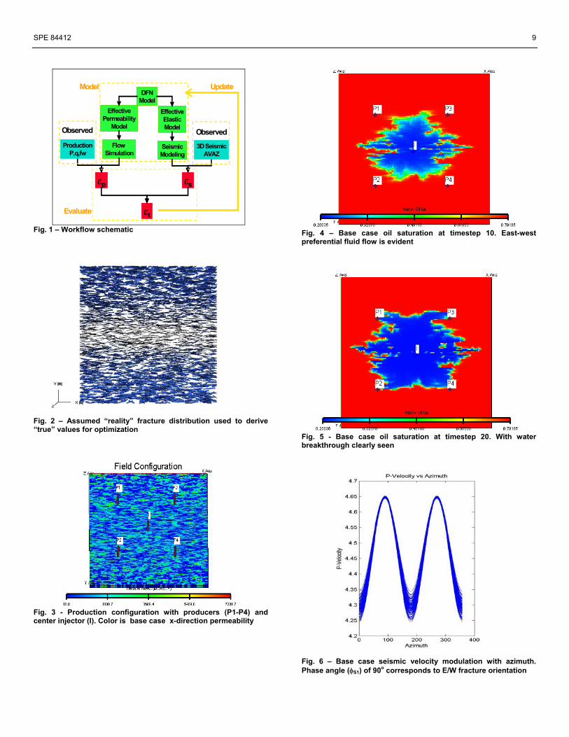
This process, illustrated in Fig. 1, is demonstrated through

a synthetic test in which a “base case” DFN model was used to represent the “true” reservoir for the purpose of creating a set of “field” observations of production and elastic data. An initial estimate of the fracture distribution was then selected to represent the results of a “well data only” characterization. The proposed optimization process was then applied to integrate seismic anisotropy with production data to optimize the model. The model was optimized in parallel using a similar approach but with production data only. Results show that integration of seismic anisotropy improves model convergence and provides better characterization of the fracture system away from the wells. Each step of this process is elaborated on in the following sections. The necessary simplifying assumptions will be discussed at each occurrence. Initial fracture and reservoir modeling Discrete feature network modeling is increasing in popularity for use as part of advanced integrated naturally-fractured reservoir characterization efforts. Given a comprehensive set of geologic, geophysical, borehole, and engineering observations, it is possible to create a conditioned stochastic estimate of the fracture system in the reservoir.

Individual fractures and systems of natural fractures may be parameterized as follows;26

Individual Fractures Systems of Fractures Orientation Sets Size Chronology Location Hierarchy Termination style Termination % Aperture Intensity Roughness Connectivity Planarity

Many of the above parameters may be determined directly

or inferred through integrated analysis of various field observations including;

• Outcrop analogs • Borehole imaging • Conventional well logs • Borehole seismic • Packer tests • Spinners • Flow meters

Integration of these data into calibration of the DFN

model assures conditioning of the model at and near the wellbore. However, such models still need to be conditioned

SPE 84412 3

in the inter-well space Lapointe27. This study assumes that a well conditioned DFN model has been created and conditioned using the data types listed above.

For this study, a synthetic base case DFN model was created (Fig. 2). The DFN was developed assuming that the reservoir was flat-lying with uniform host matrix properties. All fractures will be modeled as being vertical with constant thickness and aperture and transmissivity. Reservoir geometry and fracture system parameters are listed in Table 1 and Table 2. Table 1 – Base case fracture population parameter

Spatial pattern assumption Poisson Rectangle Fracture normal pole trend [0, 10] Normal Fracture normal pole plunge [0,0] Normal Length (m) [40,3] Lognormal Height (m) 30 Constant Fracture Intensity (P32) (m2/m3) 0.2 Constant Transmissivity (m2/s) 1.e-04 Constant

Table 2 – Rock matrix bulk properties

Matrix porosity (p.u.) 10 Matrix permeability (mD) 10

Fracture porosity (p.u.) 1.5 Vpp (m/s) 4670 Vss (m/s) 3060 ρ (g/cm3) 2.51

The parameters used for the reference DFN are

deliberately simplified. Future studies will consider more realistic geologic conditions, including fractal geometries and their implications. Effective permeability properties Dershowitz et al.28 outlined a comprehensive method for integrating DFN models into the conventional finite difference simulator workflow. For the study presented here, the effective permeability of the fracture system was computed from the DFN fracture model using Oda’s method.6,29 For a given rock volume an empirical fracture tensor is computed by weighted averaging of individual fracture areas and transmissivities.

∑=

=N

kjkikkkcij nnTA

VF

1

1 …………………… (1)

where; T = fracture transmissivity (m2/s) Ac = fracture cross-sectional area (m2) nij = unit normal vectors Transmissivity is a characteristic of the fracture and fluid system;

µρ12

3gbT = ………………………….(2)

where;

ρ = fluid density (g/cm3) µ = fluid viscosity (cp) b = fracture aperture (cm) g = acceleration of gravity (m/s2) Then, the Oda effective permeability is computed as;

( )ijijkkij FFk −= δ121

……………….(3)

Oda’s formulation has the advantage that it does not

require flow simulation, but it does not take into account fracture connectivity. Further studies in this area will utilize more sophisticated finite element modeling-based techniques for modeling the permeability of the fracture system. To reduce the effect of off-diagonal tensor components effective permeabilities were computed on a very fine (3-m) grid with one axis aligned parallel to the mean fracture direction. Gridding parameters are listed in Table 3. Table 3 – Dimensions and sampling parameters for computational grids.

Grid NX NY DX DY Effective permeability 262 262 3m 3m Simulation 131 131 6m 6m Seismic modeling 16 16 50 50

Anisotropic elastic media properties Seismic anisotropy resulting from elongated voids in the host media can be described through various models including Oda5, Kuster-Tokzos30, Hudson31, and the linear slip discontinuity model. The latter model was selected for this study because it allows computation using discrete fracture descriptions rather than fracture population statistics. Further, this model has been used by Schoenberg and Sayers as the basis for seismic anisotropy studies as referenced earlier in this paper. This model is derived from the anisotropic form of Hooke’s law,

klijklij c εσ = ……….…………………………...(4) where;

σij = stress (Pa) εkl = strain cijkl = elastic stiffness (Pa).

Equivalently, it can be expressed as

ijijklijijklkl cs σσε 1−== …………………..……..(5) where;

sijkl = elastic compliance (Pa-1) In fractured media, the compliance tensor s can be expressed as

4 SPE 84412

ijklhijklijkl sss ∆+= ………………..………..…..(6)

where;

shijkl = elastic compliance of host

media ∆s = fracture compliance

Schoenberg and Sayers have shown that the additional compliance of the medium resulting from the presence of fractures can be expressed as

( ) ijklikjliljkjkiljlikijkls βαδαδαδαδ ++++=∆41 ,...(7)

∑=r

rs

rj

ri

rTij AnnB

V)()()()('1α ,…………………….…...(8)

∑= )()()()()()('1 rs

rl

rk

rj

ri

rNijkl AnnnnB

Vβ ,………….…...(9)

where; B’N = fracture normal (Pa-1-m)

compliance B’T = fracture shear compliance (Pa-1-m) As = fracture surface area (m2) n = unit normal vectors

Given a discrete description of the fracture distribution

and knowledge of B’N and B’T in Eq. 9, Eqs. 6-9 allow modeling of the anisotropic elastic behavior of the fractured medium. For this study the reservoir was divided into a regular grid. Elastic stiffness tensors were computed for each grid block on a coarse grid (Table 3). Although no method exists for directly measuring B’N and B’T, Pyrak-Nolte20 presented experimental results of a method for estimating fracture shear stiffness from seismic interference. Sayers32 provides analytical expressions for B’N and B’T as functions of fracture aspet ratio, host medium, and fluid prioperties. Values selected for B’N and B’T generally agree with the results of computations using the Sayers analytical expression. These yield velocity anisotropy of approximately 90% for the studied DFN.

Production performance modeling Production performance from the reservoir model was predicted using a dual-porosity formulation from a proprietary software. This formulation represents the fractured reservoir as an orthogonal array of matrix blocks surrounded by fractures as described in early works by Barrenblatt et al.,33 Warren and Root,34 and Kazemi et al..35 The dual-porosity model used required calibration to provide representative results. Gurpinar and Kossak36 provided a systematic analysis of scaling issues encountered in practical usage of single and dual-porosity finite difference simulators in fractured reservoirs.

Since this study does not include the use of ‘time-lapse’ seismic observations, it is necessary to assume that fracture compressibility remains constant throughout the history

matching period. In addition, pressure support s maintained such that fracture compressibility is not changed significantly as a result of depletion effects. A library of generic fracture stiffnesses (Yip37) is availale to support this analysis in future studies.

A 10-acre 5-spot pattern with center water injector (Fig. 3) was used. The gridblock size was upscaled to reduce computational time for each update. The reservoir was produced using constant liquid rate control for 600 days. Capillary pressure and fluid parameters contained in the dual-porosity test case of Kazemi et al.38 were assumed. The reservoir fluid was undersaturated black oil. Reservoir pressure was kept above the bubble-point to maintain a two-phase system.

Oil production (OPR) and bottom-hole pressure (BHP) observations were used as the production components of the optimization objective function. Figs. 4 and 5 show oil saturation in the reservoir at two simulator report steps. Stochastic errors of 10 psi for BHP and 50 bbl/D were included to simulate random noise in computed observations. Seismic attribute modeling Directional propagation P and shear velocities for any arbitrary fractured medium can be computed from the compliance tensor given by Eqs. 5-8. This azimuthal variation in velocity results in a systematic variation in reflection amplitude at the interface of the anisotropic layer. Ikelle39 derived expressions for P-wave reflection coefficient as a function of angle and azimuth as a Fourier series in azimuth. For fracture distributions with weak anisotropy and monoclinic symmetry with horizontal plane of mirror symmetry, the azimuthal dependence of P-wave reflectivity can be written as

( ) ( )( ) ( ) ...2cos6cos

2cos,

6266

22

+−+−

+−+=

φφφφ

φφφθ

GG

GDR pp ………... (10)

where;

D = constant Gn = Fourier component

modulation amplitude θ = incidence angle φ = raypath azimuth

Coefficients and angles (φ) in Eq. 10 are functions of elastic tensor coefficients (Eqs. 8 and 9).

The above relation is frequently simplified and rearranged to obtain the well-known expression for ANMO used by Mallick et al..8

( ) )(2cos, 1Spp BAV φφφθ −+= …………….……(11) where;

Vpp = compressional wave interval Velocity

θ = incidence angle φ = raypath azimuth φs1 = fast shear azimuth

SPE 84412 5

A = constant (m/s) B = modulation amplitude (m/s)

Figs. 6 and 7 illustrate the velocity-versus-azimuth plot

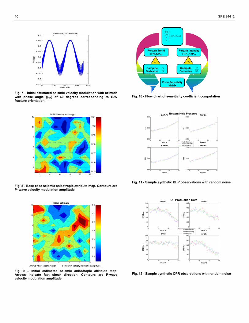
for the base case reservoir model. Shift in the phase angle (φS1) resulting from different fracture orientations is clear. For a single set of fractures with constant compliance, modulation amplitude B is proportional to the intensity of the fracture system; the direction of fast shear wave propagation, φS1, is aligned parallel with the fracture system orientation. Eq. 10 was used to parameterize elastic anisotropy in terms of B and φs1. This computation was performed for each grid block on the 2D reservoir horizon. Approximately 10% random noise was added to the synthetic seismic observations. Figs. 8 and 9 illustrate the composite seismic anisotropic attribute maps for the base model and initial model estimate. Arrows represent the fast shear direction (φS1) and the modulation amplitude (B) is contoured. Objective function The objective function for optimization is formed as a composite of mean-square terms from both production and seismic observations.

( ) ( )( ) ( ) ( )( )

( ) ( )( ) ( ) ( )( )2

1

2

1

2

1

2

1...

∑∑

∑∑

==

==

−+−+

−+−=

nw

i

conw

i

co

nw

i

cPi

oPi

nw

i

cPi

oPi

avgavgBavgBavg

OPRavgOPRavgBHPavgBHPavgQ

ϕϕ

,….. (12)

where

BHP = Bottom-hole pressure (psi) OPR = oil production rate (bbl/D) nw = number of wells φs1 = fast shear azimuth B = velocity modulation amplitude

The production penalty term was made up of a combination of BHP and OPR, with each averaged over the production history for each well as output from the reservoir simulation program. These observations were selected because wells were produced with constant liquid rate control and the reservoir was under-saturated, resulting in water production rate being directly correlated to oil production, and no gas production.

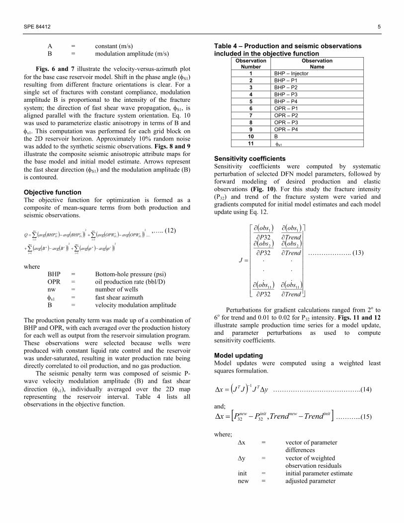
The seismic penalty term was composed of seismic P-wave velocity modulation amplitude (B) and fast shear direction (φs1), individually averaged over the 2D map representing the reservoir interval. Table 4 lists all observations in the objective function.

Table 4 – Production and seismic observations included in the objective function

Observation Number

Observation Name

1 BHP – Injector 2 BHP – P1 3 BHP – P2 4 BHP – P3 5 BHP – P4 6 OPR – P1 7 OPR – P2 8 OPR – P3 9 OPR – P4

10 B 11 φs1

Sensitivity coefficients Sensitivity coefficients were computed by systematic perturbation of selected DFN model parameters, followed by forward modeling of desired production and elastic observations (Fig. 10). For this study the fracture intensity (P32) and trend of the fracture system were varied and gradients computed for initial model estimates and each model update using Eq. 12.

( ) ( )

( ) ( )

( ) ( )

∂∂

∂∂

∂∂

∂∂

∂∂

∂∂

=

Trendobs

Pobs

Trendobs

Pobs

Trendobs

Pobs

J

1111

22

11

32

..

..

..32

32

……………….. (13)

Perturbations for gradient calculations ranged from 2o to

6o for trend and 0.01 to 0.02 for P32 intensity. Figs. 11 and 12 illustrate sample production time series for a model update, and parameter perturbations as used to compute sensitivity coefficients.

Model updating Model updates were computed using a weighted least squares formulation.

( ) yJJJx TT ∆=∆−1

………………………………….(14) and;

[ ]initnewinitnew TrendTrendPPx −−=∆ ,3232 ………...(15) where; ∆x = vector of parameter

differences ∆y = vector of weighted

observation residuals init = initial parameter estimate new = adjusted parameter

6 SPE 84412

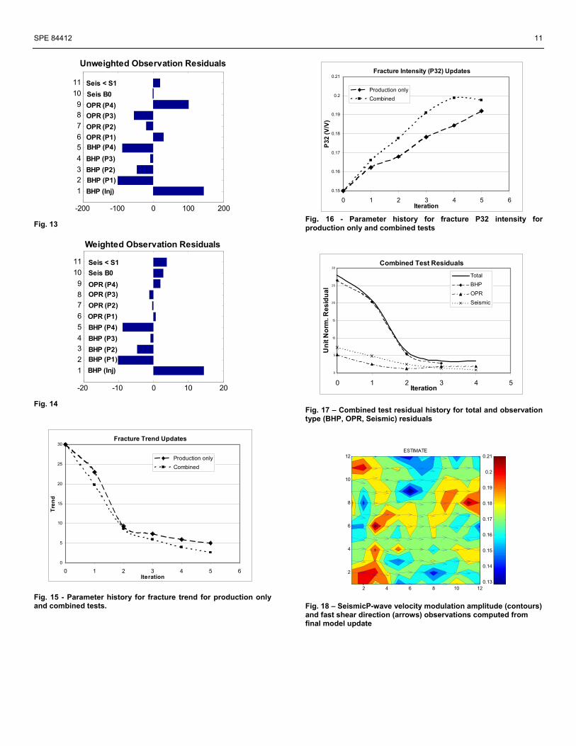
Observations were weighted in accordance with their respective noise estimates. Figs. 13 and 14 illustrate weighted and unweighted observation residuals from one update step. Prior model bias was introduced by means of scalar weighting of the sensitivity matrix columns. For the purpose of this study, the weighting factor was 0.5 for both trend and P32 intensity on all updates. Five iterations and model updates were performed for production only scheme and for combined production and seismic schemes. Results To evaluate the benefit of this process, model update tests with and without seismic were conducted in parallel. Initial estimates for fracture trend and P32 were set to 30o and 0.15m2/m3, respectively, and gradients were calculated at that point. Model gradients for subsequent updates were computed independently for each update parameter set. To account for the effects of random noise, 10 updates were computed for each new model estimate and the results were averaged. It was observed that prior model weighting was required to maintain stability of the initial update steps. Parameter perturbations for gradient computations were also reduced as convergence progressed.

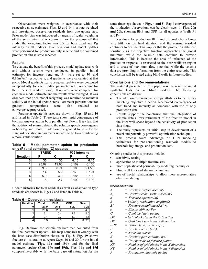
Parameter update histories are shown in Figs. 15 and 16 and listed in Table 5. These tests show rapid convergence of both parameters and in both parallel test flows. It is clear that the addition of seismic data to the solution speeds convergence in both P32 and trend. In addition, the general trend is for the standard deviation in parameter updates to be lower, indicating a more stable solution. Table 5 – Model parameter update for production only (P) and combines (C) updates

TREND P32 IntensityIteration P C P C

0 30 30 0.15 0.151 23.07 19.80 0.162 0.1662 9.3 8.74 0.168 0.17763 7.4 5.9 0.178 0.1914 5.9 4.0 0.185 0.1995 5 2.7 0.192 0.198

Update histories for total residual as well as observation type residuals are shown in Fig. 17 and listed in Table 6. Table 6 – Observation residuals

Iteration Total BHP OPR Seis0 27.9 26.41 5.22 7.251 20.8 20.2 2.5 4.82 6.1 5.4 1.2 2.53 3.4 2.7 1.9 1.44 3.3 2.6 1.8 0.820

Fig. 18 shows the seismic attribute map computed from

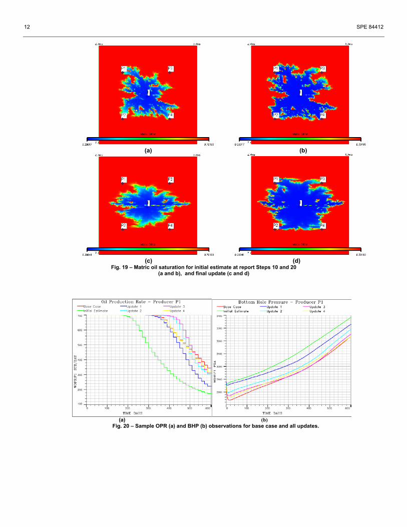
the final parameter update. This map compares favorably with the base case distribution shown in Fig. 8. Fig. 19 shows fracture oil saturation at report Steps 10 and 20 for the initial model estimate (Figs. 19a and 19b), and for the final parameter update (Figs. 19c and 19d). Figs. 19c and 19d compare favorably with the base case oil saturation for the

same timesteps shown in Figs. 4 and 5. Rapid convergence of the production observations can be clearly seen in Figs. 20a and 20b, showing BHP and OPR for all updates at Wells P1 and P4.

Residuals for production BHP and oil production change very little on the final iteration, and the seismic residual continues to decline. This implies that the production data lose sensitivity as the objective function approaches the global minimum while the seismic data continue to provide information. This is because the area of influence of the production response is restricted to the near wellbore region and to areas of maximum flow potential, while the seismic data are providing information from the entire reservoir. This conclusion will be tested using blind wells in future studies. Conclusions and Recommendations The material presented in this paper was the result of initial synthetic tests on simplified models. The following conclusions are drawn: • The addition of seismic anisotropy attributes to the history

matching objective function accelerated convergence of both trend and intensity as compared with use of only production data.

• Results support the conclusion that the integration of seismic data allows refinement of the fracture model in the inter-well space beyond the sensitivity of production data alone.

• The study represents an initial step in development of a novel and potentially powerful optimization technique.

• This process takes advantage of DFN modeling techniques for pre-conditioning reservoir models to borehole log, image, and production data.

Ongoing studies in this process include; • sensitivity testing • application to multiple fracture sets • more sophisticated permeability modeling techniques • blind well tests and streamline analysis • use of fractal relationships to allow more representative

elastic modeling. Nomenclature A = Fracture surface area(m2) Ac = Fracture cross-section area(m2) b = Fracture aperture(m) B = Velocity modulation amplitude B’ = Fracture compliance(Pa-1-m) c = Elastic stiffness(Pa) C = Combined data update DX = Grid block size in the X direction DY = Grid block size in the Y dimension BHP = Bottom hole pressure (psi) F = Fracture tensor(m/s) J = Jacobian matrix K = Fracture permeability (m/s) nij = Unit normals to fracture planes NX = Number of grid blocks in the X dimension NY = Number of grid blocks in the Y dimension P = Production data only update

SPE 84412 7

P32 = Stochastic fracture intensity (m2/m3) r = Integration radius(m) R = Reflection amplitude s = Elastic compliance (Pa-1) T = Transmissivity(m2/s) T’ = Fracture system trend (o) V = Volume(m3) Vpp = Compressional wave interval velocity x = Parameter vector y = Weighted observation residual vector ε = Elastic strain φ = Aziumuth (o) µ = Fluid viscosity(cp) ρ = Fluid density(g/cm3) σ = Stress (Pa) θ = Incidence angle(o) Subscript c = fracture opening cross section i, j = principle indices of the arbitary reference frame N = Normal s = Fracture surface ss = Shear wave o = Host media property pp = Compressional wave sl = Fast Shear T = Tangential Superscripts c = Computed h = Host media property o = Observed init = Initial estimate for update new = After linear update nw = Number of wells References

1. Dershowitz, W., Hurley, N., and Been, K.: “Stochastic Discrete Fracture Modeling of Heterogeneous and Fractured Reservoirs. Proceedings,” 1992 Third European Conference on the Mathematics of Oil Recovery, Delft.

2. Dershowitz, W., and Herda, H.H.: “Interpretation of Fracture Spacing and Intensity,” 1992 Proceedings of the 33rd U.S. Symposium on Rock Mechanics, Santa Fe, NM. 757.

3. Qui, Y., Holtz, M.H., Yang, A.: “Applying Curvature Analysis to the Placement of Horizontal Wells: Example from the Mabee (San Andres) Reservoir, Texas,” SPE paper 70010 presented at the 2001 SPE Permian Basin Oil and Gas Recovery Conference, held in Midland, Tx., May 15-16.

4. Oda, M.; “Fabric tensor for discontinuous geologic materials,” Soils Fdns (1982) 22(4), 96.

5. Oda, M., Suzuki, K., Maeshibu, T.; “Elastic compliance for rock-like materials,” Soils Fdns (1984) 24(3), 27.

6. Oda, M.; “Permeability Tensor for Discontinuous Rock Masses,” Geotechnique (1985) Vol. 35, 483.

7. Schoenberg, M.: “Reflection of elastic waves from periodically stratified media with interfacial slip,” Geophys. Prosp. (1983) 31, 265.

8. Schoenberg, M. Sayers, C.M.: “Seismic anisotropy of fractured rock,” Geophysics, (1995) Vol. 60 no. 1, 204.

9. Schoenberg, M., Douma, J.; “Elastic wave propagation in media with parallel fractures and aligned fractures,” Geophysical Prospecting (1988) Vol. 36, 571.

10. Sayers, C.M., Dean, S.: “Azimuth-dependent AVO in reservoirs containing non-orthogonal fracture sets,” Geophysical Prospecting (2001) Vol 49,. 100.

11. Sayers, C.M., Rickett. J.E.: “Azimuthal variation in AVO response for fractured gas sands,” Geophysical Prospecting Vol 45, 165.

12. Perez, M.A., Gibson, R.L.: “Detection of fracture orientation using azimuthal variation of P-wave AVO response: Barinas field (Venezuela),” Geophysics (1999) Vol. 64 no. 4, 1253.

13. Mallick, S., Craft, K., Meister, L., Chambers, R.: “Determination of the principle directions of azimuthal anisotropy from P-wave seismic data,” Geophysics (1998) Vol. 63 no. 2, 692.

14. Parney, B., LaPointe, P.: “Fractures Can Come Into Focus”, AAPG Explorer, (Oct. 2002).

15. Parney, B., LaPointe, P.: “Simple Seismic, Complex Fractures,” AAPG Explorer (Nov. 2002).

16. Brown, R.L., Gupta, A.: “Problems Calibrating Production and Seismic Data for Fractured Reservoirs,” SPE paper no. 67317 presented at the 2001 SPE Production and Operations Symposium held in Oklahoma City, Oklahoma, March, 24-27.

17. Pickup, G.E., MacBeth, C.: “Integrating Effective Flow and Seismic Properties,” presented at the EAGE/SEG Technical Conference and Exhibition held in Zurich (May 2001).

18. King, M.S., Xu, S., Shakeel, A.: “Elastic Wave Propagation and Fluid Permeability in Rocks with Systems of Natural Fractures,” Int. J. Rock Mech. Min. Sci. (1998), Vol 35 No. 4/5, 445.

19. King, M.S.: “Elastic wave propagation in and permeability for rocks with multiple parallel fractures”, Int. J. Rock Mech. Min. Sci. (2002) Vol 39, 1033.

20. Pyrak-Nolte, L.J.: “The Seismic Response of Fractures and the Interrelations among Fracture Properties,” Int. J. Rock Mech. Min. Sci. & Geomech. Abstr. (1996) Vol 33, No. 8. 787.

21. Datta-Gupta, A. Vasco, D.W., Yoon, S.: “Integrating Dynamic Data Into High-Resolution Reservoir Models Using Streamline-Based Analytic Sensitivity Coefficients,” SPE paper 59253, SPEJ (Dec 1999).

22. Landa, J.: “Technique to Integrate Production and Static Data in a Self-Consistent way,” SPE paper 71597, presented at the 2001 SPE Annual Technical Conference and Exhibition held in New Orleans La., Sept 30-Oct 3.

23. Landa, J., Horne, R.N., Kamal, M.M., Jenkins, C.D.: “Reservoir Characterization Constrained to Well-Test Data: A Field Example,” SPE Reservoir Evaluation and Engineering 3 (4) (Aug 2000).

24. Huang, X., Meister, L., Workman, R.: “Improvement and Sensitivity of Reservoir Characterization Derived From Time-Lapse Seismic Data,” accepted for presentation at the 1998 SPE Annual Technical Conference and Exhibition held in New Orleans, Louisiana, Sept 27-30.

25. Huang, X., Will, R., Waggoner, J.: “Reconciliation of Time-lapse Seismic Data with Production Data for Reservoir Management: A Gulf of Mexico Reservoir,” SPE paper 65155, presented at the 2000 SPE European Petroleum Conference held in Paris, France, Oct 24-25.

26. Dershowitz, W. et al.: “Fracman: Discrete Feature Data Analysis, Geometric Modeling, and Exploration Simulation. User Documentation, Ver. 2.6,” Golder Associates, Seattle (2003).

8 SPE 84412

27. LaPointe et al.: “3D Reservoir and Stochastic Fracture Network Modeling for Enhanced Oil Recovery, Circle Ridge Phosphoria/Tensleep Reservoir, Wind River Reservation, Arapaho and ShoShone Tribes, Wyoming: Final Technical Report – May 1, 2000 through October 31, 2002,” DOE project no. DE-FG26 OOBC15190, (Nov. 2002.

28. Dershowitz, B., Lapointe, P., Eiben, T., Wei, L.: “Integration of Discrete Feature Network Methods with Conventional Simulator Approaches,” SPE paper no. 62498 presented at the 1998 SPE Annual Technical Conference and Exhibition held in New Orleans, Louisiana, Sept 27-30.

29. Dershowitz, W. et al.: “StrataFrac; User Documentation: Linking Discrete Fracture Networks to Geocellular Grids, Version 1.0,” Golder Associates, Seattle (2002).

30. Kuster, G.T., Toksoz, M.N.: “Velocity and attenuation of seismic waves in two-phase media”, Geophys. (1974) 587.

31. Hudson, J.A.: “Wave speeds and attenuation of elastic waves in material cracks,” Geophys. J. Royal Astronom. Soc., 64, 133.

32. Sayers, C.M.; “Fluid dependent shear-wave splitting in fractured media,” Geophys. Prospecting, 50 (2002) 393.

33. Barenblatt, G.I., Zheltov, I.P., Kochina, I.N.: “Basic Concepts in the Theory of Seepage of Homogeneous Liquids in Fissured Rocks [Strata],” PMM (1960) Vol. 24, No. 5.

34. Warren, J.E., Root, P.J.: “The Behavior of Naturally Fractured Reservoirs,” The Society of Petroleum Engineering Journal, Trans. AIME (Sept 1963) Vol. 228 245.

35. Kazemi, H, Merril, L.S., Porterfield, K.L., Zeman, P.R.: “Numerical Simulation of Water-Oil Flow in Naturally Fractured Reservoirs”, SPE paper no. 5719 presented at the 1976 SPE-AIME 4th Symposium on Numerical Simulation of Reservoir Performance held in Los Angeles, California, Feb 19-20.

36. Gurpinar, O., Kossack, C.: “Realistic Numerical Models for Fractured Reservoirs,” SPE paper no. 68268 presented at the 2000 SPE International Petroleum Conference and Exhibition in Mexico held in Villahermosa, Mexico, Feb 1-3.

37. Yip, C.K.: “Shear Strength and Deformability of Rock Joints,” SM Thesis, Department of Civil Engineering, Massechusets Institute of Technology, Cambridge, MA (1979).

38. Kazemi, H, Merrill, L.S., Porterfield, K.L., Zeman, P.R.: “Numerical Simulation of Water-Oil Flow in Fractured Reservoirs,” SPEJ (1976) 317.

39. Ikelle, L.T.: “Amplitude variations with azimuth (AVAZ) inversion based on linearized inversion of common azimuth sections,” in Seismic Anisotropy, SEG, Tulsa, 601.

SPE 84412 9

DFNModel

EffectiveElasticModel

EffectivePermeability

Model

Flow Simulation

SeismicModeling

εp εs

εt

Model

Evaluate

ProductionP,q,fw

3D SeismicAVAZ

Observed Observed

UpdateDFN

ModelEffectiveElasticModel

EffectivePermeability

Model

Flow Simulation

SeismicModeling

εp εs

εt

Model

Evaluate

ProductionP,q,fw

3D SeismicAVAZ

Observed Observed

Update

Fig. 1 – Workflow schematic

Fig. 2 – Assumed “reality” fracture distribution used to derive “true” values for optimization

Fig. 3 - Production configuration with producers (P1-P4) and center injector (I). Color is base case x-direction permeability

Fig. 4 – Base case oil saturation at timestep 10. East-west preferential fluid flow is evident

Fig. 5 - Base case oil saturation at timestep 20. With water breakthrough clearly seen

Fig. 6 – Base case seismic velocity modulation with azimuth. Phase angle (φS1) of 90o corresponds to E/W fracture orientation

10 SPE 84412

Fig. 7 – Initial estimated seismic velocity modulation with azimuth with phase angle (φS1) of 60 degrees corresponding to E-W fracture orientation

2 4 6 8 10 12

2

4

6

8

10

12BASE Velocity Anisotropy

0.15

0.16

0.17

0.18

0.19

0.2

0.21

Fig. 8 - Base case seismic anisotropic attribute map. Contours are P- wave velocity modulation amplitude

2 4 6 8 10 12

2

4

6

8

10

12Initial Estimate

0.12

0.13

0.14

0.15

0.16

0.17

0.18

Arrows = Fast shear direction Contours = Velocity Modulation Amplitude Fig. 9 – Initial estimated seismic anisotropic attribute map. Arrows indicate fast shear direction. Contours are P-wave velocity modulation amplitude

∆T ∆P32

Perturb Trend(T+∆T,P32)

Perturb Intensity(T,P32+∆P32

( )TrendPfB

OPRBHP

,32=

ϕ

Tf

∂∂Compute

Derivative 32Pf

∂∂Compute

Derivative

Form SensitivityMatrix

∆T ∆P32

Perturb Trend(T+∆T,P32)

Perturb Intensity(T,P32+∆P32

( )TrendPfB

OPRBHP

,32=

ϕ

Tf

∂∂Compute

Derivative Tf

∂∂Compute

Derivative 32Pf

∂∂Compute

Derivative 32Pf

∂∂Compute

Derivative

Form SensitivityMatrix

Fig. 10 - Flow chart of sensitivity coefficient computation

0 20 40 602500

3000

3500BHP-P1

Days/10

PSI

0 20 40 602500

3000

3500BHP-P2

Days/10

PSI

0 20 40 602500

3000

3500BHP-P3

Days/10

PSI

0 20 40 602500

3000

3500BHP-P4

Days/10

PSI

Model EstimatePerturb IntensityPerturb Trend

Bottom Hole Pressure

Fig. 11 - Sample synthetic BHP observations with random noise

0 20 40 600

200

400

600

800

1000OPR-P1

Days/10

STB/

Day

0 20 40 600

200

400

600

800

1000OPR-P2

Days/10

STB

/Day

0 20 40 600

200

400

600

800

1000OPR-P3

Days/10

STB/

Day

0 20 40 600

200

400

600

800

1000OPR-P4

Days/10

STB/

Day

Model EstimatePerturb IntensityPerturb Trend

Oil Production Rate

Fig. 12 - Sample synthetic OPR observations with random noise

SPE 84412 11

-200 -100 0 100 200

123456789

1011

Unweighted Observation Residuals

BHP (Inj) BHP (P1) BHP (P2) BHP (P3) BHP (P4) OPR (P1) OPR (P2) OPR (P3) OPR (P4) Seis B0 Seis < S1

Fig. 13

-20 -10 0 10 20

123456789

1011

Weighted Observation Residuals

Seis < S1 Seis B0 OPR (P4) OPR (P3) OPR (P2) OPR (P1) BHP (P4) BHP (P3) BHP (P2) BHP (P1) BHP (Inj)

Fig. 14

Fracture Trend Updates

0

5

10

15

20

25

30

0 1 2 3 4 5 6Iteration

Tren

d

Production onlyCombined

Fig. 15 - Parameter history for fracture trend for production only and combined tests.

Fracture Intensity (P32) Updates

0.15

0.16

0.17

0.18

0.19

0.2

0.21

0 1 2 3 4 5 6Iteration

P32

(V/V

)

Production onlyCombined

Fig. 16 - Parameter history for fracture P32 intensity for production only and combined tests

Combined Test Residuals

0

5

10

15

20

25

30

0 1 2 3 4 5Iteration

Uni

t Nor

m. R

esid

ual

TotalBHPOPRSeismic

Fig. 17 – Combined test residual history for total and observation type (BHP, OPR, Seismic) residuals

2 4 6 8 10 12

2

4

6

8

10

12ESTIMATE

0.13

0.14

0.15

0.16

0.17

0.18

0.19

0.2

0.21

Fig. 18 – SeismicP-wave velocity modulation amplitude (contours) and fast shear direction (arrows) observations computed from final model update

12 SPE 84412

(a) (b)

(c) (d)

Fig. 19 – Matric oil saturation for initial estimate at report Steps 10 and 20 (a and b), and final update (c and d)

(a) (b)

Fig. 20 – Sample OPR (a) and BHP (b) observations for base case and all updates.