Integration of Depositional Process Modelling, Rock ...
109
Department of Exploration Geophysics Integration of Depositional Process Modelling, Rock Physics and Seismic Forward Modelling to Constrain Depositional Parameters Mohammed Ali O Alkaff This thesis is presented for the Degree of Master of Philosophy (Geophysics) of Curtin University of Technology March 2015
Transcript of Integration of Depositional Process Modelling, Rock ...

Department of Exploration Geophysics
Integration of Depositional Process Modelling, Rock Physics and Seismic Forward
Modelling to Constrain Depositional Parameters
Mohammed Ali O Alkaff
This thesis is presented for the Degree of
Master of Philosophy (Geophysics)
of
Curtin University of Technology
March 2015

DECLARATION
To the best of my knowledge and belief this thesis contains no material previously published by any
other person except where due acknowledgment has been made.
This thesis contains no material which has been accepted for the award of any other degree or diploma
in any university.
Signature: ………………………………………….
Date: …………31/03/2015……………...

i
ABSTRACT
Sedsim, a numerical stratigraphic forward modelling package, which quantitatively and
deterministically predicts variations in sediment distribution over time as the depositional
environment changes, was used to generate a stratigraphic model over the Cornea field, Browse
Basin, Australia. The target reservoir within the Cornea field is the Albian sandstones which form
isolated sandstone bodies within siltstones and clay-rich sediments. Although numerical stratigraphic
forward modelling is powerful technique for predicting the subsurface, it comes with uncertainty. In
order to identify and reduce the uncertainty in the stratigraphic model, this thesis proposed and
applied the method of closing the loop, where the stratigraphic model over the Cornea field was
integrated with the velocity-porosity-clay (VPC) rock physics model and the process of seismic
forward modelling.
In this study, it took thirty one runs to generate the final Sedsim model. Before each run, initial
Sedsim parameters had to be modified. Initially, during the earlier runs, uncertainty in the
stratigraphic model was easily identified just by viewing the results. Initial Sedsim parameters were
then modified accordingly. However, as the stratigraphic model became more reasonable, uncertainty
became difficult to identify.
The VPC rock physics model, which is suitable for clean sandstones as well as clay rich sandstones,
was used to convert input from the stratigraphic model to elastic parameters. The elastic parameters
were then used to calculate acoustic parameters. The acoustic parameters were used to generate
synthetic seismic data via the process of seismic forward modelling. The simulated synthetic seismic
data was then compared to its corresponding observed seismic data. The parameters of the generated
Sedsim stratigraphic model were modified based on the results of the comparison.
The process of closing the loop was successfully applied twice in this study. Once where sediments
were deposited abruptly resulting in the formation of one thick interval. It was hard to see this in the

ii
stratigraphic model but when the model was converted to seismic, uncertainty was identified by the
absence of synthetic seismic reflections within that interval compared to observe seismic and initial
Sedsim parameters were modified accordingly and the stratigraphic model was regenerated. During
the second time, closing the loop revealed problems within a carbonate interval overlaying the target.
It was concluded that once possible source for these problems was the application of the VPC rock
physics model, designed for siliciclastics, within a carbonate interval. Other possible sources of error
such as inaccurate initial Sedsim parameters are not to be excluded.
Ideally, another rock physics model, suitable for carbonate rocks, should be run within the carbonate
interval. Then, the process of closing the loop should be applied to identify the source of the problem
within the carbonate interval, whether it is from the VPC model or the initial Sedsim parameters, and
reduce uncertainty to a satisfactory degree. However, due to the limited time given for this study, this
was stated as a recommendation for future work.
Comparison between synthetic and observed seismic remained qualitative in this study. However, it
was recommended to turn it into a quantitative process by inverting observed seismic data. Hence, one
could perhaps in the future automate the process.
The process of closing the loop can be used to identify and reduce uncertainty in numerical
stratigraphic modelling. The process of closing the loop is practical in terms of identifying
uncertainty. However, finding the correct Sedsim parameters to modify in order to reduce the
identified uncertainty in addition to re-running the Sedsim model can be time consuming. The run
time problem can be overcome by reducing some Sedsim parameters such as grid size or by breaking
the modelled area into smaller parts. In addition, the process of closing the loop came with by-
products and applications that could be used utilized for other purposes.

iii
ACKNOWLEDGEMENTS
I would like to express my deep gratitude to my thesis committee, Professor Boris Gurevich, Dr.
Cedric Griffiths, Dr. Roman Pevzner, Dr. Mahyar Madadi and Dr. Maxim Lebedev for their support
and patience in achieving this work.
I would like to thank Dr. Andrej Bona for his support in writing MATLAB code.
I also thank Geoscience Australia for providing me with seismic and well log data.
Finally, I thank SAUDI ARAMCO for their sponsorship of my Master’s Degree.

iv
TABLE OF CONTENTS
ABSTRACT ............................................................................................................................................. i
ACKNOWLEDGEMENTS ................................................................................................................... iii
LIST OF FIGURES ............................................................................................................................... vi
LIST OF TABLES ................................................................................................................................ vii
LIST OF APPENDICES ...................................................................................................................... viii
CHAPTER 1 INTRODUCTION ............................................................................................................ 1
Synopsis .............................................................................................................................................. 1
1.1 Motivation ..................................................................................................................................... 1
1.2 Objective ....................................................................................................................................... 2
1.3 Workflow ...................................................................................................................................... 2
CHAPTER 2 BACKGROUND ............................................................................................................. 5
Synopsis .............................................................................................................................................. 5
2.1 Stratigraphic Forward Modelling .................................................................................................. 5
2.2 Traditional Stratigraphic (or Geo-cellular) Modelling .................................................................. 6
2.3 Numerical Stratigraphic Forward Modelling ................................................................................ 6
2.4 Sedsim Introduction ...................................................................................................................... 7
2.5 Uncertainty in Numerical Stratigraphic Forward Modelling ...................................................... 11
2.6 “Closing the loop” As A Method To Minimize Uncertainty ...................................................... 12
2.7 The Problem of Input .................................................................................................................. 13
2.8 Seismic Forward Modelling ........................................................................................................ 14
2.9 Traditional Seismic Forward Modelling ..................................................................................... 16
2.10 The Application of Rock Physics in Seismic Forward Modelling ............................................ 17
2.11 The Velocity-Porosity-Clay (VPC) Rock Physics Model Background .................................... 18
2.12 Synthetic vs. Observed Seismic Data Comparison ................................................................... 21
CHAPTER 3 STUDY AREA .............................................................................................................. 24
Synopsis ............................................................................................................................................ 24
3.1 The Cornea Field: Geological Background ................................................................................ 24
3.2 The Cornea Field: Geophysical Background .............................................................................. 28
3.3 The Cornea Field: Petrophysical Background ............................................................................ 29
CHAPTER 4 Sedsim STRATIGRAPHIC FORWARD MODELLING.............................................. 31
Synopsis: ........................................................................................................................................... 31
4.1 Sedsim Input ............................................................................................................................... 31
4.2 Sedsim Runs................................................................................................................................ 36
4.3 Sedsim Output Parameters .......................................................................................................... 42
v
4.4 Preparing Sedsim Output for Rock Physics Model..................................................................... 44
CHAPTER 5 VELOCITY-POROSITY-CLAY (VPC) ROCK PHYSICS MODEL .......................... 47
Synopsis ............................................................................................................................................ 47
5.1 VPC Compatibility to Study Area .............................................................................................. 47
5.2 VPC Compatibility to Sedsim Model ......................................................................................... 50
5.3 VPC Input Parameters ................................................................................................................. 51
5.4 VPC Output Parameters .............................................................................................................. 52
CHAPTER 6 SEISMIC FORWARD MODELLING .......................................................................... 55
Synopsis ............................................................................................................................................ 55
6.1 Calculating Acoustic Parameters ................................................................................................ 55
6.2 Synthetic Seismic data display method ....................................................................................... 59
CHAPTER 7 SYNTHETIC VS. OBSERVED SEISMIC DATA COMPARISON ............................ 60
Synopsis ............................................................................................................................................ 60
7.1 Observed Seismic vs. Sparse 2D Synthetic Seismic ................................................................... 60
7.2 Observed Seismic vs. Partial 3D Synthetic Seismic ................................................................... 62
7.3 Observed Seismic vs. Final 3D Synthetic Seismic ..................................................................... 65
CHAPTER 8 CONCLUSIONS AND RECOMMENDATIONS ........................................................ 67
Synopsis ............................................................................................................................................ 67
8.1 The Main Objective .................................................................................................................... 67
8.2 Secondary Objectives .................................................................................................................. 69
8.3 By-products ................................................................................................................................. 70
8.4 Assumptions ................................................................................................................................ 71
8.5 Conclusions ................................................................................................................................. 72
8.6 Recommendations ....................................................................................................................... 74
8.7 Possible Future Work .................................................................................................................. 74
REFERENCES ..................................................................................................................................... 75
APPENDICES ...................................................................................................................................... 79

vi
LIST OF FIGURES
FIGURE 1.1: A CHART SUMMARIZING THE WORKFLOW OF THIS STUDY .................................................. 3
FIGURE 2.1: AN ILLUSTRATION OF SEDSIM COMPUTATIONAL MODULES ............................................... 9
FIGURE 2.2: SEDSIM USER-INPUT DATA ................................................................................................ 10
FIGURE 2.3: SEDSIM STRATIGRAPHIC MODEL EXAMPLE. ...................................................................... 11
FIGURE 2.4: CLOSING THE LOOP. .......................................................................................................... 12
FIGURE 2.5: THE PROBLEM OF INPUT ................................................................................................... 14
FIGURE 2.6: SEISMIC FORWARD MODELLING ........................................................................................ 15
FIGURE 2.7: A SIMPLE TWO-LAYER EARTH MODEL. .............................................................................. 16
FIGURE 3.1: THE CORNEA FIELD LOCATION.......................................................................................... 24
FIGURE 3.2: TARGET RESERVOIR: ALBIAN SANDS................................................................................ 26
FIGURE 3.3: CORNEA-1 AND 1B WELL LOGS ......................................................................................... 28
FIGURE 3.4: WELLS WITHIN AND AROUND THE CORNEA FIELD ............................................................ 30
FIGURE 4.1: A SOUTH-NORTH LINE THROUGH CORNEA OBSERVED 3D SEISMIC DATA ........................ 36
FIGURE 4.2: TOP VIEW OF SEDSIM STRATIGRAPHIC MODEL FROM RUN 2 ............................................ 37
FIGURE 4.3: TOP VIEW OF SEDSIM STRATIGRAPHIC MODEL FROM RUN 9 ............................................ 38
FIGURE 4.4: LINES THROUGH SEDSIM STRATIGRAPHIC MODEL FROM RUN 9 ....................................... 39
FIGURE 4.5: LINES THROUGH STRATIGRAPHIC MODEL FROM SEDSIM RUN 16 ..................................... 39
FIGURE 4.6: TOP VIEW OF SEDSIM RUN 31 ........................................................................................... 40
FIGURE 4.7: FINAL SEDSIM STRATIGRAPHIC MODEL (RUN 31) ............................................................. 41
FIGURE 4.8: TOP VIEW OF SEDSIM STRATIGRAPHIC MODEL FROM RUN 31 .......................................... 41
FIGURE 4.9: ILLUSTRATION OF SEDSIM NODES ..................................................................................... 43
FIGURE 5.1: CORNEA-1 PREDICTED VS. ACTUAL STRATIGRAPHY ......................................................... 49
FIGURE 5.2: A SOUTH-NORTH LINE THROUGH CORNEA OBSERVED 3D SEISMIC DATA ........................ 50
FIGURE 5.3: GRAIN SIZE AND TOTAL POROSITY FROM SEDSIM. ............................................................ 53
FIGURE 5.4: BULK MODULUS, SHEAR MODULUET AL.S AND DENSITY AT EACH DEPTH INTERVAL ....... 54
FIGURE 6.1: ACOUSTIC AND SHEAR IMPEDANCE AT EACH DEPTH INTERVAL ....................................... 56
FIGURE 6.2: APPLYING THE CONVOLUTIONAL MODEL ......................................................................... 58
FIGURE 6.3: REFLECTION COEFFICIENTS AT EACH SEDSIM NODE ......................................................... 59
FIGURE 7.1: OBSERVED SEISMIC TRACE VS. SYNTHETIC SEISMIC TRACE .............................................. 61
FIGURE 7.2: SIDE VIEW OF SEDSIM MODEL ........................................................................................... 62
FIGURE 7.3: A COMPARISON BETWEEN SYNTHETIC AND OBSERVED SEISMIC DATA ............................. 64
FIGURE 7.4: GENERATED SYNTHETIC SEISMIC VOLUMES. .................................................................... 66
FIGURE 8.1: SEABED TIME HORIZON OVER THE CORNEA FIELD ............................................................ 72

vii
LIST OF TABLES
TABLE 4.1: SUMMARY OF SIZE, LITHOLOGY AND MINERAL OF SEDSIM GRAIN SIZES ........................... 44
TABLE 5.1: BULK AND SHEAR MODULI AND DENSITY VALUES USED IN THIS STUDY............................ 51

viii
LIST OF APPENDICES
APPENDIX A: MAIN CODE ..................................................................................................................... 79
APPENDIX B: VPC ROCK PHYSICS MODEL CODE ................................................................................ 83
APPENDIX C: SEDSIM FILE READING CODE .......................................................................................... 85
APPENDIX D: INDEX CODE .................................................................................................................... 86
APPENDIX E: SEDSIM FINAL INPUT TEXT FILE ..................................................................................... 87
APPENDIX F: SEDSIM OUTPUT FILE (ONE TRACE EXAMPLE) IN .CSV FORMAT ..................................... 94
APPENDIX G: GEOSCIENCE AUSTRALIA COPYRIGHT STATEMENT ....................................................... 95
APPENDIX H: GEOSCIENCE AUSTRALIA COPYRIGHT PERMISSION ....................................................... 96
APPENDIX I: CEDRIC GRIFFITHS COPYRIGHT PERMISSION ................................................................... 97
APPENDIX J: SEGYMAT COPYRIGHT STATEMENT ............................................................................... 98
APPENDIX K: DEPOSITIONAL ENVIRONMENT DESCREPTION ................................................................ 99

1
CHAPTER 1
INTRODUCTION
Synopsis
This chapter summarizes the motivation, objectives and workflow of this study. More details are
available in the next chapters.
1.1 Motivation
Stratigraphic forward modelling (SFM) is a technique for predicting subsurface geology away from
well data. Traditional stratigraphic forward modelling utilizes all available data including well logs
and seismic interpretation. Then, “unknown gaps” in the subsurface geology e.g. at inter-well location
are filled using geo-statistical methods such as interpolation and krigging (Bohling, 2005). In areas,
where the wells are scarce or far apart or areas where there are significant lateral variations in the
subsurface geology, geo-statistical methods are associated with significant uncertainty (Yarus, 2009).
Another type of stratigraphic forward modelling is numerical stratigraphic forward modelling.
Numerical stratigraphic forward modelling attempts to predict the subsurface deterministically;
starting at user-specified geologic time, numerical stratigraphic forward modelling software simulates
depositional processes as time progresses from the user-specified geologic time to present time
(Griffiths & Dyt, and Griffiths et al., 2001). However, many runs are required in order to create a
reasonable stratigraphic model using this method. The resultant stratigraphic model needs to be
assessed after each run. In other words, the uncertainty must be minimized after each run until
satisfactory results are achieved. Therefore, a method via which uncertainty can be assessed and
minimized is needed.
One way of evaluating the uncertainty of a numerical stratigraphic model is by generating synthetic
seismic data from the stratigraphic model. The synthetic seismic data is then compared to
corresponding observed seismic data over the same area. Based on the comparison results, initial

2
input parameters within the stratigraphic model are modified and the model is regenerated. This
process is repeated until satisfactory results are achieved i.e. until uncertainty in the stratigraphic
model is minimized. In this study, this process of generating a numerical stratigraphic model,
generating synthetic seismic data from it, comparing it to its corresponding observed seismic data,
regenerating the model based on the comparison results is referred to as closing the loop. This process
is repeated until uncertainty in the model is minimized.
Al-Siyabi, Gurevich, and Madadi (2012) attempted to generate synthetic seismic data by integrating
the VPC rock physics model and an existing Sedsim-generated stratigraphic model. They found that
the use of a low resolution stratigraphic model and a rock physics model that is unsuitable for the
geological properties output by the stratigraphic model can negatively impact the generated synthetic
seismic.
1.2 Objective
The main objective behind this study is to minimize uncertainty in the numerical stratigraphic model
by closing the loop. During the process of closing the loop, synthetic seismic data, to be compared to
observed seismic data, is generated from the stratigraphic model. Therefore the process of closing the
loop allows for indirect comparison of the resultant numerical stratigraphic forward model with
observed seismic data.
As secondary objectives, the final generated stratigraphic model can be used to constrain the number
of possible realizations in stochastic inversion. In addition, many products that are generated during
the process of closing the loop can be utilized for different applications.
1.3 Workflow
The first step in the workflow is to select a study area i.e. a geographical location where the study can
be carried out. Once a study area is selected, a numerical stratigraphic forward modelling program is
used to generate a numerical stratigraphic model over the study area. The program used in this study

3
is Sedsim. Sedsim was originally developed by Harbaugh’s group in the 1980s at Stanford University.
It has been enhanced by CSIRO group at the University of Adelaide since 1994 (Griffiths & Dyt, and
Griffiths et al., 2001).When an initial Sedsim model is generated, it is converted to synthetic seismic
(Figure 1.1).
Figure 1.1: Workflow Chart: A chart summarizing the workflow of this study. First, a study
area is selected. Then, a stratigraphic model over the selected area is generated. Geological
parameters from the stratigraphic model are inputted into a rock physics model to generated
elastic parameters. These are then used to calculate acoustic parameters. The acoustic
parameters are converted to synthetic seismic via seismic forward modelling. Finally, the
synthetic seismic data is compared with the observed seismic data.
In order to convert the generated Sedsim model to synthetic seismic, an existing rock physics model is
utilized. The rock physics model is used to convert geological properties from the Sedsim model to
elastic properties. These elastic properties as used to calculate acoustic properties. Via seismic
forward modelling, the acoustic properties are used to generate synthetic seismic data.
When synthetic seismic data is finally generated, it is compared to observed seismic data over the
same area, the study area. Sedsim initial parameters are modified based on this comparison and the
Stratigraphic Model
Rock Physics Model
Seismic Forward
Modelling
Geological Parameters
Elastic Parameters
3D Synthetic Seismic
Acoustic Parameters
3D Observed Seismic
Compare

4
program is re-run to generate an updated Sedsim model. This process, closing the loop, is repeated
until a “good match” between synthetic and observed data is achieved i.e. the uncertainty in Sedsim
model is minimized.

5
CHAPTER 2
BACKGROUND
Synopsis
This chapter illustrates the research plan via which the objective is achieved. In addition, it reviews
some basic concepts needed to understand the objective.
2.1 Stratigraphic Forward Modelling
Stratigraphic modelling can be used to predict the subsurface. It attempts to create a three dimensional
representation or a realization of an area of the subsurface based on geological and geophysical
observations. Geological observations usually include data from well logs while geophysical
observations are usually based on the interpretation of seismic data.
A modern stratigraphic modelling program should be able to integrate all available data in order to
create a model of rock layering and properties at some required resolution in three dimensions
(Fallara, Legault & Rabeau, 2006). Some programs start by building a structural framework using
interpretation results e.g. fault polygons and horizons from seismic data. Well log data are then
incorporated in the model to add information on geological properties such as porosity, lithology and
fluid saturation (Yarus, 2009).
The stratigraphic model is divided into a number of cells. The more cells, the higher resolution of the
stratigraphic model and the finer the features it can resolve.
When all available geological and geophysical data are incorporated into the stratigraphic model, geo-
statistical methods are used to populate these cells. Geo-statistical methods such as interpolation and
kriging are used to fill in the gaps in areas where there is no data (Bohling, 2005).

6
2.2 Traditional Stratigraphic (or Geo-cellular) Modelling
Since the 1980’s oil-field stratigraphic modelling (‘static modelling’) has primarily used geo-
statistical methods.
A typical task for a traditional modelling approach is to interpolate sediment properties between two
or more wells by applying geo-statistical methods using data from these wells as input. Other types of
input including seismic data, and previously known geological information, are also utilized. In this
case the accuracy of the stratigraphic model is usually dependent on the quality and availability of
input data. Therefore, in areas where data is of relatively low quality or quantity, the resultant
stratigraphic model comes with large uncertainty (Yarus, 2009).
2.3 Numerical Stratigraphic Forward Modelling
Unlike traditional stratigraphic modelling, numerical stratigraphic forward modelling does not rely on
geo-statistical methods. A numerical SFM program is able to quantitatively model the changes in
sedimentation process with time in order to predict rock properties away from well data. A numerical
SFM program usually starts with a given geological time and geological parameters. It then simulates
the sedimentation process as time progresses and as the depositional environment changes (Griffiths
& Dyt, and Griffiths et al., 2001).
A numerical SFM program divides the stratigraphic model into cells similar to those created by a
traditional stratigraphic modelling program. However, these cells are not populated using geo-
statistical methods. Instead, they are populated deterministically using palaeo-environment and
palinspastic reconstruction knowledge over a user-specified geological time interval rather than depth
intervals (Griffiths & Dyt, and Griffiths et al., 2001).
The deterministic approach of numerical forward stratigraphic modelling makes it less reliant on the
availability of geological and geophysical data at well locations. In addition, it reduces possible bias
towards “hard data” such as well logs, which can result in uncertainty in areas with sparse wells or

7
where there are large subsurface variations. Consequently, numerical stratigraphic forward modelling
comes with uncertainty that is more uniform and testable than traditional stratigraphic geo-cellular
modelling (Griffiths & Dyt, and Griffiths et al., 2001).
Numerical stratigraphic Forward Modelling (NSFM) is a sedimentary process simulation that replays
the way that stratigraphic successions develop and are preserved. It reproduces numerically the
physical processes that eroded, transported, deposited and modified the sediments over varying time
periods. In a forward modelling approach, data are not used as the anchor points for facies
interpolation or extrapolation, but to test and validate the results of the simulation. Stratigraphic
forward modelling is an iterative approach, where input parameters have to be modified until the
results are validated by actual data. One of the major benefits of using NSFM to characterize
sedimentary successions is the fact that, unlike with geo-statistical approaches, the results will always
make sense from a geological point of view. It is also possible to test different geological scenarios,
environments or conceptual models, to assess their impact on the stratal geometry and better
understand the depositional processes. Ultimately, it enables the prediction of facies and porosity
distributions in areas where data are sparse, unevenly distributed, or at inappropriate resolution
(Griffiths & Dyt, and Griffiths et al., 2001).
2.4 Sedsim Introduction
Sedsim is a three-dimensional stratigraphic forward modelling program. It was originally developed
in the 1980s at Stanford University by D. Tetzlaff and J. Wendebourg under the supervision of Prof. J.
Harbaugh. Since 1994, the program has been undergoing modifications and enhancement at the
University of Adelaide and at the Commonwealth Scientific and Industrial Research Organization
(CSIRO) by C. Dyt, F. Li and T. Salles (Griffiths & Dyt, and Griffiths et al., 2001).
Sedsim is at its core a numerical hydraulic-process based computer program. This means that Sedsim
quantitatively predicts variations in sediment distribution over geological time as the depositional
environment changes. This is achieved deterministically by applying fluid flow equations to a range

8
of geological parameters determined from palaeo-environment and palinspastic reconstructions over a
user-specified geological time interval (Griffiths & Dyt, and Griffiths et al., 2001). In other words,
Sedsim starts at a user-specified geological time and replays the sedimentation processes as geological
time progresses and as depositional environment changes. The program can simulate various
siliciclastic and carbonate depositional processes on a given bathymetric surface.
Sedsim employs approximations to solutions of the Navier-Stokes equations in order to numerically
simulate fluid flow and sediement erosion, transport and deposition. The full Navier-Stokes equations
are currently impossible to solve. Therefore the equations are simplified within Sedsim and are solved
using a marker-in-cell approach using a combined Eulerian and Lagrangian representation of fluid
flow. The fluid flow is simulated in two horizontal dimensions while flow velocities are assumed to
be uniform in the vertical direction (so-called 2D-depth-averaged flow). In this case, the velocity of
the fluid body as a whole remains constant but can change in horizontal directions. Fluid flow velocity
and sediment load are represented by points within the fluid body that move with the flow. At a given
time, a point or marker contains information including fluid flow velocity, sediment load and fluid
element position. This information is recalculated and updated at each time step (Griffiths & Dyt, and
Griffiths et al., 2001).
Within Sedsim there are core programs and sub-programs or computational modules. The core
programs are related to fluid flow and sedimentation. Some of the computational modules are linked
to the core programs while others are executed separately. The computational modules include
subsidence, sea level change, wave transport, compaction, slope failure, carbonates and organics
(Figure 2.1) (Griffiths & Paraschivoiu, 1998).
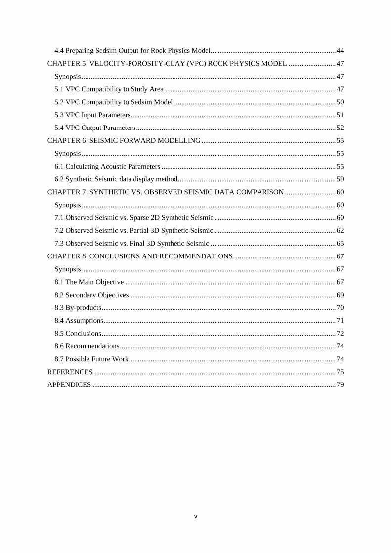
9
Figure 2.1: An illustration showing computational modules that are linked to Sedsim core
program (Sea Level, Wave Transport, Compaction and Subsidence) and computational
modules that are run separately (Turbidite Flow, Aeolian Deposition and Carbonate
Deposition).
In addition to core programs and modules, user-input data, which control fluid flow and sedimentation
processes, can be fed into Sedsim. The user-input data can be divided into two parts: Sedsim
parameters and additional input. Each module in Sedsim contains a set of parameters that can be
specified or modified by the user. These parameters include (among many others) sediment and river
source location, fluid density, fluid velocity, wave direction, and sea level curve (Griffiths &
Paraschivoiu, 1998). Many of these parameters can be derived from the literature while others involve

10
iterative testing until Sedsim output matches well and seismic stratal geometries to an acceptable
degree.
Sedsim does not use well logs or seismic horizons as input data but a seismic horizon is often used as
a starting or basal surface, a bathymetric surface on which Sedsim begins the hydraulic flow process.
This surface may be initially derived from a seismic horizon representing e.g. an unconformity
surface but it often needs some palinspastic reconstruction to correctly reflect hydraulic flow gradients
and directions (Figure 2.2) (Griffiths and Dyt, 2001).
Figure 2.2: Sedsim user-input data includes parameters within Sedsim modules such as Waves
and Sea Level. In addition, user-input may include a seismic-derived surface, base horizon, on
which Sedsim can begin the hydraulic flow process.
Several runs are usually required before Sedsim output matches observations to a pre-specified degree
at well locations. Before each run, initial input parameters are modified through a text file. The text
file is run in Sedsim. The result, the stratigraphic model, is generated in the form of a set of files and
is displayed using the SedView viewer external to Sedsim. The computational time and intensity for
Sea level
Sediment supply
Waves
Griffiths, 2014
Base Horizon

11
each run varies depending on the input parameters and input data. A large grid size, or many modules,
for example, will increase the computational time and intensity (Griffiths & Dyt, 2001).
The resultant Sedsim stratigraphic model is three-dimensional grid node volume; the vertical axis is in
either depth or geological time, the horizontal axes are in distance while the value at each node is a
selected geological property such as porosity, grain size and geological age. Each node in the model
has a UTM coordinate location and contains quantitative information concerning geological properties
such as porosity and grain size at different depths (Figure 2.3). The number of the nodes and the
distance between them are specified in the input parameters (Griffiths & Dyt, 2001).
Figure 2.3: Sedsim stratigraphic model example: the vertical axis is depth in meters, the
horizontal axes are distance in meters and the node values are: lithofacies (top-left), alternating
age (top-right), lithology (bottom-left) and porosity (bottom-right).
2.5 Uncertainty in Numerical Stratigraphic Forward Modelling
Although numerical stratigraphic forward modelling is a powerful technique, it is important to
constrain and minimise the uncertainty in the resultant stratigraphic model. The process of creating a
stratigraphic forward model using a numerical stratigraphic forward modelling program usually

12
requires several runs before Sedsim output matches observations to a pre-specified degree at well
locations. Before each run, initial input parameters are modified. A process is needed in order to
determine whether the output is satisfactory and which parameters to modify. In other words, we need
a process by which the uncertainty in the output can be constrained.
2.6 “Closing the loop” As A Method To Minimize Uncertainty
One approach to reducing the uncertainty in a stratigraphic model is by comparing it to observed
seismic data. The stratigraphic model is then modified based on the results of the comparison.
However, a comparison between a stratigraphic model and observed seismic is not valid since the two
are of different parameters. This problem can be overcome by simulating synthetic seismic data from
the stratigraphic model. The simulated synthetic seismic data is then compared to observed data over
the same area. This allows for a comparison between the results of the stratigraphic model and the
observed seismic data, which in turn can be used to tune or modify the initial parameters of the
stratigraphic model (i.e., closing the loop) and thus reduce the uncertainty of the stratigraphic model
(Figure 2.4).
Figure 2.4: Uncertainty in the stratigraphic model can be minimized by closing the loop:
comparing synthetic seismic data derived from a stratigraphic model with corresponding
observed seismic data and modifying the initial stratigraphic model parameters based on the
results of the comparison.

13
The process of closing the loop is usually repeated several times until a satisfactory result is obtained
i.e. until a satisfactory match between the simulated synthetic seismic and the observed seismic is
obtained.
2.7 The Problem of Input
So far, I have proposed comparing the generated stratigraphic model to observed seismic as a method
to reduce the uncertainty in the stratigraphic model. As explained above, this is done via the process
of closing the loop: simulating synthetic seismic data from the stratigraphic model. One can then
compare the generated synthetic seismic data to the observed seismic data. The stratigraphic model is
then modified until a good match between the two data sets, synthetic and observed, is achieved.
One problem that may arise during such comparison is what I like to refer to as the “problem of
input”. During the generation of a stratigraphic forward model, geophysical data mainly from the
observed seismic data are used as initial input. This means that the stratigraphic forward model will be
influenced by input data from the observed seismic before any comparison is made. Consequently, a
good match between synthetic seismic data (generated from the stratigraphic forward model) and
observed seismic data could be a result of the geophysical input data from the observed seismic and
not necessarily an indication of the accuracy of the stratigraphic forward model (Figure 2.5).

14
Figure 2.5: The Problem of Input: When observed seismic data is used initially as input into the
stratigraphic model, it is passed to the synthetic seismic data generated from the stratigraphic
model. Therefore, any match or mis-match between synthetic and observed seismic data may be
attributed to initial observed seismic input and not to the quality of the stratigraphic model.
Geophysical data used in this simulation consisted of one seismic horizon corresponding to one
reflection boundary in the observed seismic data and to the base of a stratigraphic layer. This horizon
is used as base level on top of which the stratigraphic model is built. The remaining layers in the
stratigraphic model, which are above this horizon, are deterministically generated without any seismic
input. In addition, no other type of seismic or seismic-derived attribute input is used in the generation
of the stratigraphic forward model. This way, any match or mismatch between synthetic seismic
generated from the stratigraphic model data and observed seismic data is indicative of the accuracy of
the stratigraphic forward model and not a result of geophysical input from observed seismic.
2.8 Seismic Forward Modelling
A 3D seismic volume consists of seismic traces. Each one of these traces consists of a series of
amplitudes. Seismic amplitude results from the convolution of a wavelet and a reflection coefficient at
an earth boundary. A reflection coefficient at an earth boundary is calculated if the velocities and
densities above and below the boundary are known.

15
Seismic forward modelling is the process by which synthetic seismic data is generated. Therefore, in
seismic forward modelling, we usually start from an earth model and use it to generate seismic data.
Figure 2.6 below illustrates how a seismic trace is generated from an earth model through the
convolutional model (Kearey, Brooks & Hill, 2002).
Figure 2.6: Seismic forward modelling starts with a geological model. If velocities and densities
of each layer within the geological model are known, acoustic impedance (I) can be calculated
for each layer. Reflection coefficients (R) can then be calculated at each boundary. Reflection
coefficients can be used to calculate to calculate a reflectivity function. A seismic trace is the
output of the convolution (*) of a wavelet (Ricker Wavelet in this case) with the reflectivity
function. Note that the seismic trace in this figure is not generated from the geological model in
the figure. It is only used to illustrate the general concept of the convolutional model.
For further clarification, a double-layered earth model is considered where there are two distinct
subsurface layers: layer 1 and layer 2. If layer 1 has a velocity 𝑉1 and density 𝜌1, while layer 2 has a
velocity 𝑉2 and density 𝜌2 (Figure 2.7).

16
Figure 2.7: A simple two-layer earth model.
The reflection coefficient 𝑅 at the boundary between the two layers can be calculated using the
equation:
𝑅 =𝐼2 − 𝐼1
𝐼2 + 𝐼1 (1)
where 𝐼1, known as the acoustic impudence of layer 1, is the product of the velocity and density of
layer 1 and 𝐼2, the acoustic impedance of layer 2, is the product of the velocity and density of layer 2.
Once the reflection coefficient is calculated, then it can be convolved with a wavelet e.g. a Ricker
wavelet in order to generate seismic amplitude and hence seismic trace or a pulse in this case.
The example above shows that knowledge of velocity and density at each layer is necessary to
calculate acoustic impendences at each layer and thus generate seismic data. Since this is an example,
I assume that both velocity and density at each layer are known from the earth model but this is not
usually the case.
2.9 Traditional Seismic Forward Modelling
Let’s consider the same example above. Only this time, let’s assume we have a 3D stratigraphic
model instead of the simplistic double-layered earth model above and from which, we are trying to
generate a 3D synthetic seismic volume instead of a single trace. A stratigraphic model usually
contains information on the subsurface geologic parameters e.g. density. Therefore, density values can

17
be derived from the stratigraphic model. However, stratigraphic models do not usually contain
subsurface velocity information. Traditionally, well log data has been utilized in order to overcome
this problem. Well logs, namely sonic logs, can provide measurements of the velocity of the
subsurface around the borehole location (Anderson & Cardimona). Geo-statistics e.g. interpolation is
then utilized for inter-well locations. A velocity volume or cube is then generated based on the results
of geo-statistics. Velocity values from the velocity cubed are then multiplied with their corresponding
density values from the stratigraphic model to generate an acoustic impedance volume. The acoustic
impedance volume is utilized to calculate a reflectivity volume and finally the reflectivity volume is
convolved with a wavelet in order to generate the desired output: a synthetic seismic volume. This
example, again, shows that velocity information is central to seismic forward modelling. It also
illustrates one approach to get velocity information, the traditional approach, which mainly utilizes
well log data and geo-statistical methods.
Geo-statistical methods have been accepted as a way to “fill in the gaps” and sometimes give good
results. However, they can be associated with large uncertainty, especially in situations where the
subsurface velocities have significant lateral variation and where there are only a few or no wells.
Therefore, a more deterministic approach of determining the subsurface velocities is needed.
2.10 The Application of Rock Physics in Seismic Forward Modelling
Rock physical methods attempt to find a link between geological properties and geophysical
properties of rocks. This is done via a rock physics model. A rock physics model usually consists of
an equation or a set of equations, which attempt to link the geological and geophysical properties of
rocks for a given geological scenario. Various rock physics models have been derived for various
geological scenarios but they share the same basic method. They usually start with some knowledge
of the geological properties of the rock such as the constituent mineral components and porosity.
They, then, use this knowledge to calculate the elastic properties of rocks. The elastic properties of
rocks a rock physics model usually calculates are the Bulk modulus Κ, the shear modulus μ and the
density ρ. The elastic properties are then used to calculate geophysical properties i.e. velocities. The

18
elastic parameters can be calculated for various saturation scenarios by the fluid substitution method
using Gassmann’s equation (Avseth, Mukerji & Mavko, 2005).
Let’s go back to the previous example, where we are starting with a 3D stratigraphic model and would
like to use to generate a synthetic seismic volume. Only this time instead of calculating a velocity
cube using well log data and geo-statistical methods, we use a rock physics model. In this case, for
each node in 3D the stratigraphic model, we can use known geological properties e.g. consistent
mineral components and porosity as input for the rock physics model. The rock physics model can
then use these geological properties to calculate elastic parameters. These elastic parameters can then
be used to calculate velocities. Velocity values at each node can be multiplied by their corresponding
density values to calculate acoustic impedance values. Acoustic impendence values are used to
calculate reflectivity. Finally, reflectivity is convolved with a wavelet to generate a synthetic seismic
trace for each node of the 3D stratigraphic model. Since each node location corresponds to a seismic
trace location, a synthetic seismic volume can be generated by repeating this process for each node in
the 3D stratigraphic model.
The advantage of applying a rock physics model in determining the subsurface velocities is that,
unlike geo-statistical methods, it is a deterministic approach that is independent of well log data
availability. Consequently, it comes with less uncertainty compared to geo-statistical methods
especially in areas where wells are sparsely located or there are large subsurface velocity variations.
2.11 The Velocity-Porosity-Clay (VPC) Rock Physics Model Background
The Velocity-Porosity-Clay (VPC) rock physics model is an extension of the Velocity-Porosity rock
physics model proposed by Krief et al. Krief et al. Velocity-Porosity model works well for clean
porous fluid-saturated rocks. It assumes that the compressional and shear velocities of such rocks
obey Gassmann’s equations with the Biot compliance coefficient. In particular, Krief et al. Velocity-
Porosity model assumes that the Bulk Biot compliance coefficient can be given by a function of
porosity (Goldberg & Gurevich, 1998):

19
1 − 𝐵 = (1 − 𝛷𝑡𝑜𝑡𝑎𝑙)𝐴
(1−𝛷𝑡𝑜𝑡𝑎𝑙) (2)
, where 𝐵 is the Biot compliance coefficient, 𝛷𝑡𝑜𝑡𝑎𝑙 is the total porosity and 𝐴 is a dimensionless
empirical coefficient.
Therefore, given porosity information, the model can be used to calculate the compressional and shear
velocities of clean porous fluid-saturated rocks using Gassmann’s equations and the standard
compressional and shear velocities formulae (Goldberg & Gurevich, 1998):
𝐾𝑠𝑎𝑡 = 𝐾𝑑𝑟𝑦 + 𝐵2 𝑀 (3)
µ𝑠𝑎𝑡 = µ𝑑𝑟𝑦 (4)
𝑀 = (𝐵 − 𝛷𝑡𝑜𝑡𝑎𝑙
𝐾𝑠 +𝛷𝑡𝑜𝑡𝑎𝑙𝐾𝑓𝑙𝑢𝑖𝑑
)
−1
(5)
𝑉𝑝 = √(𝐾𝑠𝑎𝑡 +
43 µ𝑠𝑎𝑡)
𝜌𝑠𝑎𝑡 (6)
𝑉𝑠 = √µ𝑠𝑎𝑡
𝜌𝑠𝑎𝑡 (7)
𝜌𝑠𝑎𝑡 = 𝜌𝑒𝑓𝑓𝑒𝑐𝑡𝑖𝑣𝑒 (1 − 𝛷𝑡𝑜𝑡𝑎𝑙) + 𝜌𝑤𝑎𝑡𝑒𝑟 𝛷𝑡𝑜𝑡𝑎𝑙 (8)
, where 𝐾𝑑𝑟𝑦 and 𝐾𝑠𝑎𝑡 are the bulk moduli of the dry and saturated rocks, respectively, 𝐵 is Biot
compliance coefficient, 𝑀 is the pore-space modulus, µ𝑑𝑟𝑦 and µ𝑠𝑎𝑡 are the shear moduli of the dry
and saturated rocks, respectively, 𝛷𝑡𝑜𝑡𝑎𝑙 is the total porosity, 𝐾𝑠 is the solid grains bulk modulus,

20
𝐾𝑓𝑙𝑢𝑖𝑑 is the bulk modulus of the saturating fluid, 𝑉𝑝 is the compressional wave velocity, 𝑉𝑠 is the
shear wave velocity, 𝜌𝑠𝑎𝑡, 𝜌𝑒𝑓𝑓𝑒𝑐𝑡𝑖𝑣𝑒 and 𝜌𝑤𝑎𝑡𝑒𝑟 are the densities of the saturated rock, effective
solid rains and the saturating fluid, respectively.
In order to be able to use Krife et al. Velocity-Porosity model for clay-rick fluid saturated rocks, the
VPC model assumes that the bulk and shear moduli of the grain material and the dependence of
compliance on porosity are both functions of clay content. The first assumption is achieved by
computing a non-porous mixture of sand and clay using the lower Hashin-Shtrikman bound (Goldberg
& Gurevich, 1998):
𝐾𝑒𝑓𝑓𝑒𝑐𝑡𝑖𝑣𝑒 = 𝐾𝑐𝑙𝑎𝑦 +(1 − 𝐶)(𝐾𝑠𝑎𝑛𝑑 − 𝐾𝑐𝑙𝑎𝑦)
1 + 𝐶(𝐾𝑠𝑎𝑛𝑑 − 𝐾𝑐𝑙𝑎𝑦)/(𝐾𝑐𝑙𝑎𝑦 +43
µ𝑐𝑙𝑎𝑦) (9)
µ𝑒𝑓𝑓𝑒𝑐𝑡𝑖𝑣𝑒 = µ𝑐𝑙𝑎𝑦 +(1 − 𝐶)(µ𝑠𝑎𝑛𝑑 − µ𝑐𝑙𝑎𝑦)
1 + 𝐶(µ𝑠𝑎𝑛𝑑 − µ𝑐𝑙𝑎𝑦)/(µ𝑐𝑙𝑎𝑦 +43 µ𝑢)
(10)
, where 𝐾𝑒𝑓𝑓𝑒𝑐𝑡𝑖𝑣𝑒, 𝐾𝑠𝑎𝑛𝑑 and 𝐾𝑐𝑙𝑎𝑦 are the bulk moduli of the effective rock, sand and clay
respectively, µ𝑠𝑎𝑛𝑑 and µ𝑐𝑙𝑎𝑦 are the shear moduli of sand and clay, respectively, 𝐶 is clay content
and µ𝑢 =3
2(
1
µ𝑐𝑙𝑎𝑦+
10
9𝐾𝑐𝑙𝑎𝑦+8µ𝑐𝑙𝑎𝑦)
−1
.
The second assumption is achieved by re-writing the empirical constant A in Krief et al. compliance-
porosity function as:
𝐴 = 𝐴0 + 𝐴1𝐶2 (11)

21
, where 𝐴 is Krief’s empirical constant, 𝐴0 and 𝐴1 are empirical constants introduced by the VPC
model and 𝐶 is clay content.
Hence, introducing clay content as a parameter within Krief et al. compliance-porosity function. Like
Krief et al. Velocity-porosity model, the VPC model obeys Gassmann’s equations with the Biot
compliance coefficient. Therefore, the VPC model can be used to calculate compressional and shear
velocities for clay-rich sands using Gassmann’s equations and the standard compressional and shear
velocities formulae, as well (Goldberg & Gurevich, 1998).
Some parameters used as input for the VPC model are determined using available data within the area
of interest. In particular, 𝐾𝑐𝑙𝑎𝑦, µ𝑐𝑙𝑎𝑦 and 𝐴0 are determined using a multivariable non-linear
regression fit. Therefore, the VPC model is semi-empirical (Goldberg & Gurevich, 1998):
𝑆 =1
𝑁∑{[𝑉P
𝑁
𝑖=1
(𝜙𝑖, 𝐶𝑖) − 𝑉P𝑖]2 + 𝜔[𝑉S(𝜙𝑖, 𝐶𝑖) − 𝑉S𝑖]2} (12)
, where 𝑆 is the mean-square deviation, 𝑉P(𝜙, 𝐶 ) and 𝑉S(𝜙, 𝐶 ) are the compressional wave and shear
wave velocities calculated using the VPC model, respectively, 𝜙 is porosity, 𝐶 is clay content, 𝜔 is a
dimensionless constant that defines the weight given to shear wave velocities compared to
compressional wave velocities.
2.12 Synthetic vs. Observed Seismic Data Comparison
A comparison between two seismic volumes is not as simple as it may sound. In fact, it can be
complex. In this study there are two main factors that contribute to the complexity of such problem.
These factors are the fact that this is a comparison between synthetic seismic and observed seismic
data and that a quantitative comparison method is desired.

22
Synthetic and observed seismic inevitably differ in some aspect, no matter how great the match
between them. This is because synthetic seismic data is “ideal” i.e. it is usually free of noise such as
linear noise and multiples whereas observed seismic data is not. This can be illustrated by generating
a synthetic seismic trace from well log data and comparing this generated trace to its corresponding
observed one. Although the synthetic seismic trace may accurately represent the subsurface and more
importantly corresponds to the observed seismic trace, the two traces will probably look different.
Consequently, a comparison between synthetic and seismic data cannot be “strict”. In other words, a
good match between synthetic and observed seismic data does not necessarily require that the two
data sets, synthetic and observed, look exactly the same. However, for a good match, the two data sets
must not look too different. Based on the above, the definition I have so far for a “good match”
between synthetic and observed seismic data is that they don’t necessarily have to look exactly the
same but they must not look too different. A better and more quantitative definition is needed. This
leads us to the second main factor.
The other main factor that contributes to the complexity of the comparison between synthetic and
observed seismic data is the desire to have a quantitative method of comparison between them. A
quantitative method of comparison expresses the comparison results in terms of numbers.
One quantitative method of comparison between two seismic data sets is trace-by-trace cross
correlation. In this method, each trace from a seismic data set is cross correlated with its
corresponding trace in the other seismic data set. The result of the comparison is expressed by a
number. The higher the number the better the match. A cut-off number can be chosen for this method
below which, no good match is achieved.
Unfortunately, since the comparison in this study is between two data sets that will inevitably differ
even when a good match is achieved, cross correlation may not work. This is because cross
correlation may be too strict, assigning values that are too low for cases where there is a good match.

23
A better way to compare observed and synthetic seismic data is by first inverting observed seismic
data to acoustic impedance. The observed acoustic impedances are then compared with the synthetic
acoustic impedances. Due to time constrains, the observed seismic data is not inverted. Therefore, the
comparison is qualitative while quantitative observed versus synthetic acoustic impedance
comparison is listed as a recommendation for future work.

24
CHAPTER 3
STUDY AREA
Synopsis
This chapter is an overview of the study area in terms of the most relevant existing geological,
geophysical and petrophysical data.
3.1 The Cornea Field: Geological Background
The Cornea Field is an unproduced offshore oil field located within the inner part of the Browse basin
and across the Yampi shelf in the northwestern part of Australia (Figure 3.1). Albian sediments within
the Cornea field overlay relatively shallow Pre-Aptian Basement forming a four-way dip closure
(Moby Oil and Gas Ltd, 2009).
Figure 3.1: The Cornea field is an offshore field situated within the Browse basin, NW of
Australia (left). The field is covered by 3D seismic data and the study area was selected within
the 3D seismic coverage (right). © Commonwealth of Australia (Geoscience Australia) 2015.
This product is released under the Creative Commons Attribution 4.0 International Licence.
http://creativecommons.org/licenses/by/4.0/ (edited).

25
Since the 1997 Cornea-1 discovery well, the Albian sandstones within the Cornea Field and the
Browse basin, have become a target for hydrocarbon exploration.
Albian sediments in this area range from siltstones to sandstones. The Albian sandstones form isolated
sandstone bodies within siltstones and clay-rich sediments (Figure 3.2). In addition, some of these
sandstones are non-hydrocarbon bearing. Thus, detecting the Albian sandstones and predicting their
hydrocarbon reservoir potential is challenging (Moby Oil and Gas Ltd, 2009).

26
Figure 3.2: Target Reservoir: Albian (Ab) sands form the main target within the Cornea field.
They form sandstone bodies (yellow) within shale and siltstones (blue). © Commonwealth of
Australia (Geoscience Australia) 2015. This product is released under the Creative Commons
Attribution 4.0 International Licence. http://creativecommons.org/licenses/by/4.0/ (edited).
27
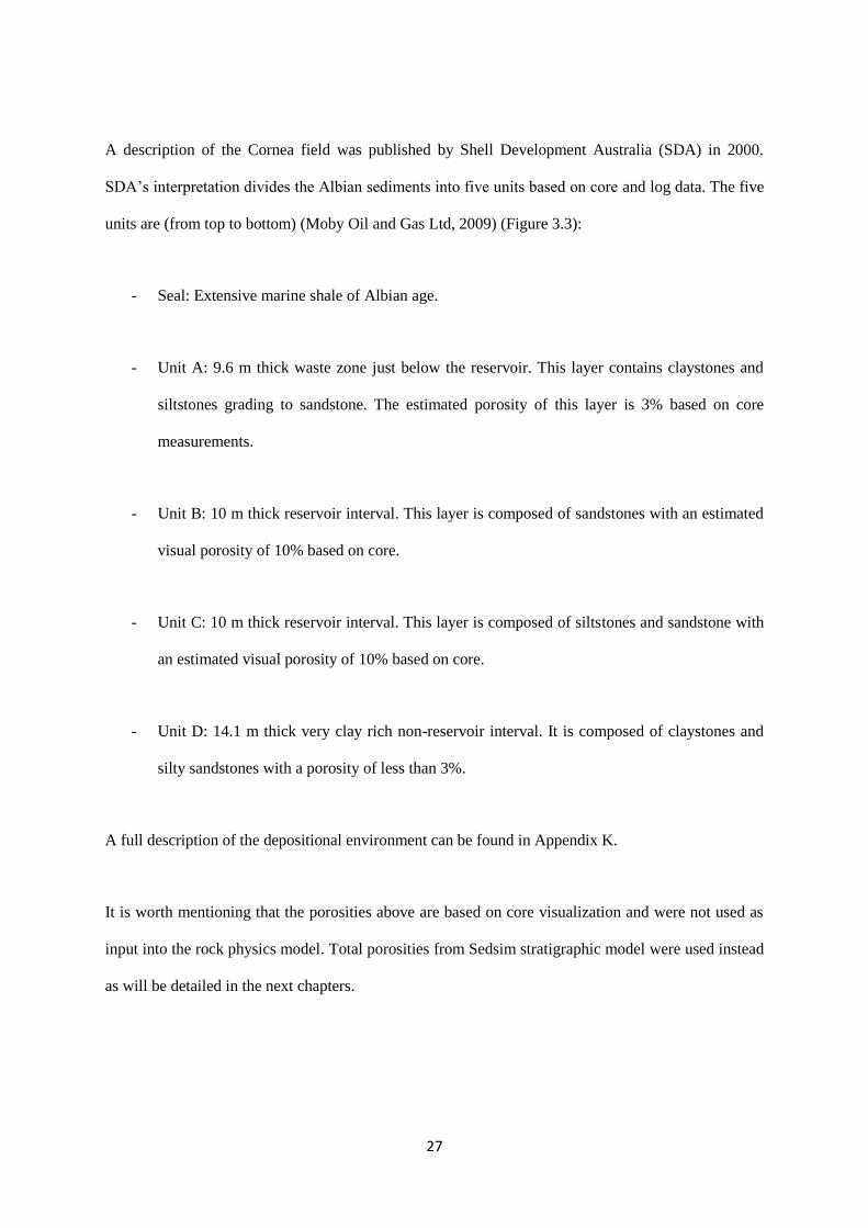
A description of the Cornea field was published by Shell Development Australia (SDA) in 2000.
SDA’s interpretation divides the Albian sediments into five units based on core and log data. The five
units are (from top to bottom) (Moby Oil and Gas Ltd, 2009) (Figure 3.3):
- Seal: Extensive marine shale of Albian age.
- Unit A: 9.6 m thick waste zone just below the reservoir. This layer contains claystones and
siltstones grading to sandstone. The estimated porosity of this layer is 3% based on core
measurements.
- Unit B: 10 m thick reservoir interval. This layer is composed of sandstones with an estimated
visual porosity of 10% based on core.
- Unit C: 10 m thick reservoir interval. This layer is composed of siltstones and sandstone with
an estimated visual porosity of 10% based on core.
- Unit D: 14.1 m thick very clay rich non-reservoir interval. It is composed of claystones and
silty sandstones with a porosity of less than 3%.
A full description of the depositional environment can be found in Appendix K.
It is worth mentioning that the porosities above are based on core visualization and were not used as
input into the rock physics model. Total porosities from Sedsim stratigraphic model were used instead
as will be detailed in the next chapters.

28
Figure 3.3: Cornea-1 and 1B well logs showing the five Albian units. © Commonwealth of
Australia (Geoscience Australia) 2015. This product is released under the Creative Commons
Attribution 4.0 International Licence. http://creativecommons.org/licenses/by/4.0/

29
3.2 The Cornea Field: Geophysical Background
The discovery well was drilled in 1997 based on a flatspot observed in 2D seismic data. The flatspot
turned out to be an oil-gas contact at well Cornea-1. Later during the same year, 2100 square
kilometres of 3D seismic data were acquired by SDA over the Cornea structure. The 3D data was
reprocessed by Hawkstone in 2008. The reprocessing of the data resulted in multiple energy
reduction. The 3D seismic data are of reasonable quality. The Pre-Aptian Basement can easily be
mapped as it shows as a strong seismic trough event across the 3D data. It, however, steeply dips in
strike and dip directions (Moby Oil and Gas Ltd, 2009).
3.3 The Cornea Field: Petrophysical Background
Several wells were drilled within or around the Cornea field since 1997. These wells include Cornea-
1, Cornea-1A, Cornea-1B, Cornea-2, Cornea-3, Cornea South-1, Cornea South-2, Tear-1, Stirrup-1,
Focus-1, Macula-1, Hammer-1, Sparkle-1, and Londonderry-1 (Figure 3.4). Wireline logs including
Gamma Ray log, Porosity log, resistivity log and sonic log were collected from some of these wells.
In addition, cores were cut in some of these wells (Geoscience Australia, 1997).

30
Figure 3.4: Wells within and around the Cornea field shown on the seabed time horizon.
Petrophysical data were mainly utilized for seismic interpretation i.e. time horizon picking of the Pre-
Aptian Basement.

31
CHAPTER 4
Sedsim STRATIGRAPHIC FORWARD MODELLING
Synopsis:
This chapter shows how Sedsim stratigraphic forward modelling software was used. It explicitly
shows the input and output to the software. In addition, it shows how the final results from Sedsim
were prepared for use in the VPC rock physics model.
4.1 Sedsim Input
As mentioned previously, Sedsim input can be divided into two types: Sedsim parameters, which exist
within the computational modules and can be user-modified, and additional input, which mainly
comprises acquired data within the area of study (Griffiths & Paraschivoiu, 1998).
Within a Sedsim input text file (Appendix E), each computational module is listed followed by its
adjustable input parameters. Initially, most of these input parameters are set to default values. Some of
the computational modules are initially “commented” or “turned off”. This means that they will not be
utilized in the construction of the stratigraphic model. In this study, to generate a stratigraphic model
over the specified area of the Cornea field, some Sedsim computational modules where used while
others were not utilized. The computational models utilized are:
TIME: the Time module contains three important parameters: The Simulation Interval (start and end
times of simulation), the Display Interval and the Flow Sampling Interval. The Simulation Interval is
specified in terms of geological time e.g. one million years ago (-1000000) and is dependent on the
geological interval to be modelled. In this study, the interval to be modelled extends from pre-Albian
basement level (> 113 million years ago) all the way to the seabed. The initial Sedsim simulations ran
from the Aptian seismic marker at 120 million years ago to the Turonian sediments (98 million years
ago) which includes the Albian (113 Ma to 100.5 Ma) reservoir interval of interest in the ‘Upper
Heywood Fm.’. The Display Interval determines interval in years at which the results files are

32
updated, while the Flow Sampling Interval determines the interval in years at which fluid elements are
released from the river source. The smaller these numbers are the higher the time resolution of the
simulation but the longer the computational time. These two parameters were initially set at 500000
and 100000 years, respectively, to give rapid results at a resolution greater than the number of seismic
reflections observed in the section from Basement to surface (around 20). This gave 72 preserved
layers at the location of Cornea-1.
GRID: The grid spacing for the generated Sedsim stratigraphic model determines the spatial
resolution of the model. The stratigraphic model will be used to generate synthetic seismic, and the
synthetic seismic data will, in turn, be compared to the observed Cornea 3D seismic data over the
same area within the Cornea field. For the two seismic data sets, synthetic and observed, to be
comparable, the grid spacing is chosen while taking into account the acquisition parameters and the
resolution of the observed 3D seismic data. In particular, grid spacing is chosen based on the CDP
spacing of the observed Cornea 3D seismic. Therefore, the regional grid spacing was initially set to
500 meters. Sedsim can also model a fine grid nested within the regional grid at a specified location.
The resolution of this fine grid was set to 50 m.
SEDIMENTS: The Sediments routine allows the user to specify the input grain size, density and
mode of transportation (suspension of bed-load) of sediments to be transported into the simulation
area. Sedsim uses four clastic grain categories: Coarse, Medium, Fine and Finest. For each of these
four categories, the user can specify a grain size in millimetres, the density in kilograms per cubic
meters and choose whether the mode of transportation will be suspension or bed-load. The grain size
for each category was chosen based on the Udden-Wentworth scale and the Cornea-1 cuttings
description. The grain densities were taken from literature for the minerals recorded in the cuttings
and core descriptions. The mode of transportation was assumed to be suspension.

33
POROSITY TABLE: The Sedsim input porosity table allows the user to specify how initial
porosities for sediment of varying mixtures respond to burial pressure. The default porosity table in
Sedsim input text file was used.
SOURCE: Source defines the flow parameters of sediment sources (usually rivers or beaches). These
parameters include Source Location, flow height, Velocity at Source, Discharge Rate, Sediment
Concentration and Sediment Composition. Six source points were specified in this study. Source 1
was located based on a previously published Sedsim study within the Browse basin. This source was
located in the eastern part of the study area. Sources 2 through 6 were added based on Sedsim runs
results. These were located in the eastern, southern, northern, western and eastern parts of the study
area, respectively. The parameters of each source were modified also based on the run results
throughout the study.
The depositional environment was considered when locating the sources. The initial source locations
from 120 Ma to 112 Ma reflected the erosion of the Cornea high providing sediment laterally to the
NW of Cornea and into the valley to the SE of the high (source 5), the more sand-rich sediment
flowing NNE to SSW along the Cornea valley to the SE of the high (source 4) and sediment provided
from the eastern coast-line across the coastal plain (source 6)
Sources 1 and 2 from 112 to 56 Ma (following the major transgression) were restricted to the eastern
part of the simulation (entering the simulation area from the east with a lower sand content and higher
flow rates from the continent. Source 3 reflected sediment from the SE flowing towards the Cornea
area along the coastal margin through longshore currents into the “Tetracantha islands” area.
Based on information from the wells and regional studies we know the marine temperature conditions
for carbonate deposition. Based on that information we know that after 56 Ma the deposition within
the Cornea field is dominated by carbonates. Carbonates are never turned off in this Sedsim
simulation but the temperature conditions for growth control their deposition.

34
PARAMETRIC SAMPLING INTERVAL: Parametric Sampling Interval is the time interval in
years at which sea level curve, wave influence, compaction and other parameters are sampled or
calculated. The smaller the Parametric Sampling Interval the higher the resolution of the model but
the longer the computational time. The Parametric Sampling Interval was set to 100000 years to
match the flow sampling interval.
SEDIMENT TRANSPORT PARAMETERS: Contains parameters that can better control the
sediment transport process. These parameters are Maximum Depth of Fluid Elements, Minimum
Velocity of Fluid Elements and Load at Source. Sedsim default values for these parameters were used.
SEA LEVEL: The 2012 Haq et al. eustatic sea level curve was used to provide accommodation
control in addition to tectonic subsidence because the core data from the Cornea field indicated an
open marine environment.
TECTONICS: Tectonic subsidence was controlled with the file “cornea_112-
0Ma_linear_subsidence_36x68.tec” which allowed four discrete subsidence intervals, A. from 122
Ma to 72 Ma, (Albian to top Campanian) B. 72 Ma to 53 Ma, (Maastrichtian to Early Eocene) C. 53
Ma to 1 Ma (Tertiary carbonate regime), D. 1 Ma to present (sediment starved transgression).
Faults are simulated based on knowledge from literature and data using the TECTONICS module. In
this study, the simulation was set to start from the Pre-Aptian Basement to sea level. We know from
literature and simple interpretation of seismic data that faults die at the basement in the Cornea field.
Therefore, no faults were simulated.
COMPACTION: Sedsim calculates compaction based on a table, which contains porosity (and
thickness) reduction values as a function of burial stress (pressure in MPa) and grain sorting (Porosity
Table in Appendix E). Consequently, compaction is controlled by pressure and grain size mixture for
each display interval. Post-depositional compaction can be applied after simulation. Parameters within

35
the Compaction module including depth of post-depositional burial by sediment and water were
estimated as 100 meters and 83 meters, respectively, based on Cornea field well reports.
The change of porosity with depth is included in all stages of the simulation, both during depositional
loading and post-depositional burial. This effectively combines the processes that influence mass
volume reduction and porosity/permeability reduction with both elapsed time and depth. The final
porosity volume reduction with depth table used in this study can be found in POROSITY TABLE in
the Sedsim input file (Appendix E). The columns represent the effect of burial pressure from zero to
50 MPa on the porosity and volume reduction for ratios of clay to sand of zero to unity. This table can
be compiled from published or proprietary studies and/or calibrated against available well data (core
and/or wireline). In this study, initially, the default one was used and the final one was determined
during Sedsim runs.
The porosity reduction will usually be a combination of compaction and diagenesis. Porosity
enhancement can also include sub-seismic fracture effects as well as diagenesis. In Sedsim, for
specific locations, such effects can be included both by using the POROSITY routine above and
within the CARBONATES AND ORGANICS module where diagenesis can affect porosity in clastics
and carbonates without rock volume changes as a function of elapsed time in years.
Other Sedsim input consisted of the initial bathymetric/topographic surface. This was a seismic time
surface representing the Pre-Aptian Basement. It was picked on the observed Cornea 3D seismic data
as a strong trough seismic event (Figure 4.1). The Pre-Aptian Basement surface resolution was
modified using the ‘Transform’ program in order to be able to use it within Sedsim. No other data
were used as input for this study.

36
Figure 4.1: A south-north line through Cornea observed 3D seismic data. The line shows the
Pre-Aptian Basement (yellow), the Turonian unconformity (green) and seabed (blue). The Pre-
Aptian Basement was picked as a 3D time horizon (corner).
4.2 Sedsim Runs
It took approximately thirty runs until a reasonable Sedsim stratigraphic model was finally generated.
The results of each run guided the decision of which parameters to be modified. Initially as the results
were clearly unreasonable, the parameters were adjusted without going through the process of closing
the loop. The process of closing the loop was utilized when the results became more reasonable i.e. as
errors became harder to spot.
The thirty Sedsim runs are summarized in four batches as follows:
Sedsim Runs 1-2: A Pre-Aptian Basement bathymetry surface covering the whole study area (brown)
was used. Source 1 was added. Major areas were not covered by sediment flow: a problem of non-
deposition (Figure 4.2).
A A’
A
A’
N

37
Figure 3.2: Top view of Sedsim stratigraphic model from Run 2 showing the location of Source
1 (S1). Sediments were deposited in the western part of the study area on the Pre-Aptian
Basement bathymetry surface (brown surface) whereas the rest of the area remained without
deposition.
Sedsim Runs 3-9: Two more sources were added, Source 2 and Source 3 in the central and western
parts of the study area, respectively, while Source 1 was move to the west. Adding these sources
partially solved the problem of non-deposition (Figure 4.3).

38
Figure 4.3: Top view of Sedsim stratigraphic model from Run 9 showing the new location of
Source 1 (S1) and the location of Sources 2 (S2) and 3 (S3). The addition of Sources 2 and 3
expanded the area of sediment deposition. The southwestern part of the study area remained
without deposition.
Sedsim Runs 10-16: Waves module was turned on. The problem of non-deposition was solved but
there was an interval where sediments were deposited abruptly resulting in the formation of one thick
layer. Based on an initial closing-the-loop run, this was not supposed to be the case; finer layers
within that thick layer should have been deposited (Figure 4.4 & Figure 4.5).

39
Figure 4.4: Lines through Sedsim stratigraphic model from Run 16 in terms of lithology.
Figure 4.5: Left: lines through stratigraphic model from Sedsim Run 16 in terms of alternating
age. Right: a single line through the same run showing a thick layer, which was deposited
abruptly (pointed by white arrow). The line was converted to synthetic seismic and compared to
its corresponding observed seismic line. The comparison showed that thin layers were supposed
to be deposited within the thick layer.
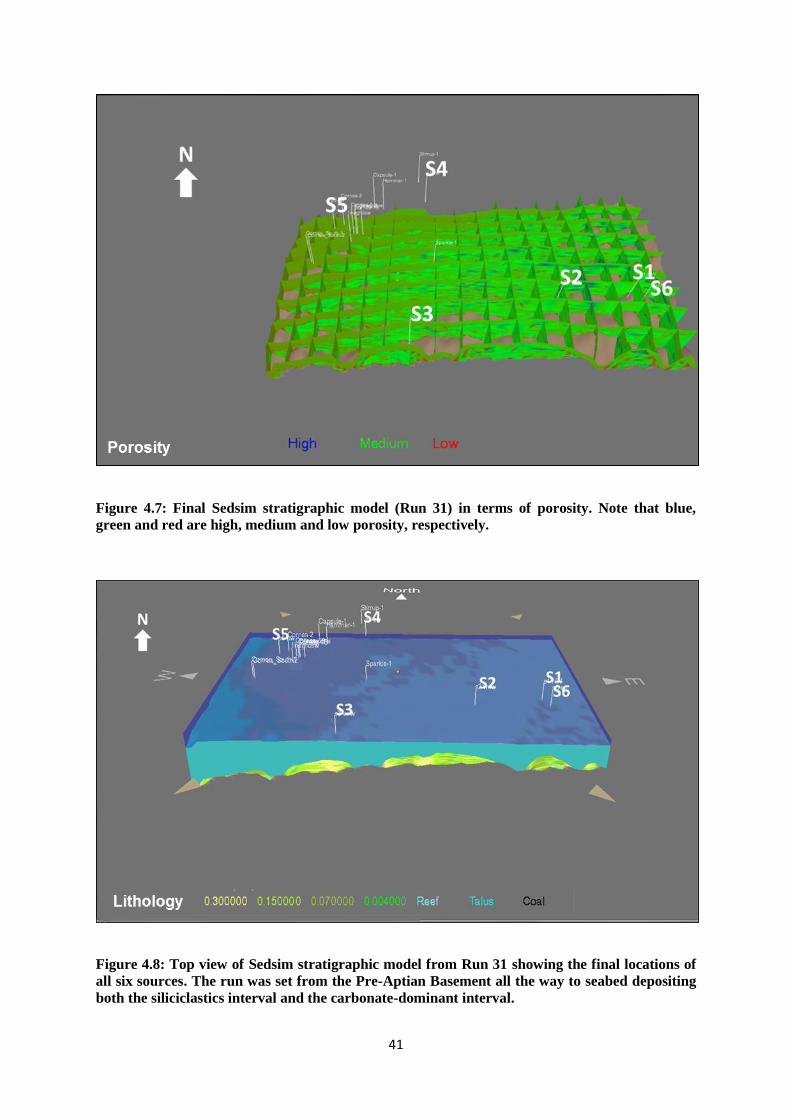
Sedsim Run 17-31: Three more sources were added. These were Sources 4, 5 and 6 in the northern,
western and eastern parts of the study area, respectively. This run was set to start from the Pre-Aptian
Basement all the way to seabed. In addition, the locations of Sources 1, 2 and 3 were modified. The

40
problem of absence of deposited layers was resolved and this run was taken as the final run (Figures
4.6 to 4.8).
Figure 4.6: Sedsim Run 31: A. Top view of Pre-Aptian Basement bathymetry surface showing
the final locations of the six sources. B. The bathymetry surface as water starts to flow. C.
Deposition of sediments from above the Pre-Aptian Basement to the Turonian Unconformity. D.
Deposition of sediments from the Turonian Unconformity to Seabed.
41
Figure 4.7: Final Sedsim stratigraphic model (Run 31) in terms of porosity. Note that blue,
green and red are high, medium and low porosity, respectively.
Figure 4.8: Top view of Sedsim stratigraphic model from Run 31 showing the final locations of
all six sources. The run was set from the Pre-Aptian Basement all the way to seabed depositing
both the siliciclastics interval and the carbonate-dominant interval.

42
The above summary highlights important changes that were made during the runs. For more details
including all changes made during each run see the top part of the input text file (Appendix E). In
addition, note that run 11 was utilized for testing purposes and therefore was not included in the text
file.
4.3 Sedsim Output Parameters
Sedsim divides the stratigraphic model into a number of nodes. On a horizontal “slice” of the
stratigraphic model, each node can be thought of as a point. On a vertical line passing through a node,
the node looks like a well-log starting from the shallowest depth of the stratigraphic model and ending
at the bottom depth of the model. The vertical line of the node is divided into intervals of depth or
“blocks”, which are generated at preserved geological time intervals. For example, although a new
depth interval can be created every ten thousand years not all of the time intervals have sediment
deposited at that time at that location, or not eroded later. The number of nodes, the distances between
them and the geological time interval are user-specified (Figure 4.9).

43
Figure 4.9: Illustration of Sedsim nodes: Sedsim stores output in a series of nodes (red circles).
Each node can be thought of as a vertical log (red line), which contains geological properties at
each depth interval (marked by the black ticks).
Each node contains quantitative information on the geological properties of the stratigraphic model at
the node location. Sedsim output is represented as a text file containing information in a tabular
format. A simple example of one node from a simulation is shown in Appendix F. The file may
contain information relating to one or more nodes as required. The information includes:
The location of the node in terms of column and row as well as Xutm and Yutm coordinates.
The elapsed time interval for each depth interval or block.
The geological time of each depth interval or block.
The length of each depth interval or block.
The component proportion of each grain size 𝑔𝑟 within each depth interval/block. These are:
(𝑔𝑟1(𝑚)), (𝑔𝑟2(𝑚)), (𝑔𝑟3(𝑚)), (𝑔𝑟4(𝑚)), (𝑔𝑟5(𝑚)), (𝑔𝑟6(𝑚)), (𝑔𝑟7(𝑚)) and (𝑔𝑟8(𝑚))
(Table 4.1).
Depth
Geological Properties e.g.
Grain size, ФTotal
Sedsim Node

44
The porosity within each depth interval/block.
The top depth of each depth interval/block.
The bottom depth of each depth interval/block.
The number and the location of nodes to be output in the text file can be specified in Sedsim.
Grain Size (millimeters) Lithology Mineral
gr1 0.3 Coarse sandstone Quartz
gr2 0.15 Medium sandstone Quartz
gr3 0.07 Fine to very fine sandstone Quartz
gr4 0.004 Very fine clay Clay
gr5 Carbonate Calcite
gr6 Carbonate Calcite
gr7 Organic Matter Calcite
gr8 Organic Matter Calcite
Table 1.1: Summary of size, lithology and mineral each grain size within Sedsim represents.
4.4 Preparing Sedsim Output for The VPC Rock Physics Model
Sedsim gives two main initial input parameters required by the VPC rock physics model (Goldberg &
Gurevich, 1998). One of them is the porosity within each depth interval. This parameter is given
directly. The other parameter, the volume fraction of the constituent minerals within each depth
interval, however, is not given directly and is calculated. Instead of giving the volume fraction of each
mineral, Sedsim gives thickness of each grain size (𝑔𝑟1 (𝑚) to 𝑔𝑟8 (𝑚)) within each depth interval.
As shown in Table 4.1, a grain size or a group of grain sizes represent certain lithology. For example,
the group 𝑔𝑟1 (𝑚), 𝑔𝑟2 (𝑚) and 𝑔𝑟3 (𝑚) represent thickness of different sizes of sandstones. In this
study, we assume that each lithology type corresponds to one mineral e.g. sandstones correspond to
quartz. This information can be used in order to calculate constituent minerals volume fractions of
each mineral at each depth interval as follows:

45
The fraction value for each grain size is calculated. This is done by calculating the sum of all grain
size thicknesses 𝑔𝑟1 (𝑚) to 𝑔𝑟8 (𝑚) for a depth interval. Then, dividing grain size thickness for
which grain size fraction is to be calculated, by the calculated sum. For example, in order to determine
the grain size fraction gf1 for grain size gr1, all grain size thicknesses from gr1 to gr8 are summed.
Then, gf1 is calculated by dividing grain size thickness gr1 by the calculated sum:
𝑔𝑓1 =𝑔𝑟1
𝑔𝑟1 + 𝑔𝑟2 + 𝑔𝑟3 + 𝑔𝑟4 + 𝑔𝑟5 + 𝑔𝑟6 + 𝑔𝑟7 + 𝑔𝑟8 (13)
, where 𝑔𝑓1 is the grain size fraction of grain size 1 and 𝑔𝑟1 to 𝑔𝑟8 are grain sizes 1 to 8.
The same process is repeated for the rest of the grain sizes to calculate grain size fractions for the
remaining grain sizes. The general form of equation (13) is:
𝑔𝑓𝑥 =𝑔𝑟𝑥
𝑔𝑟1 + 𝑔𝑟2 + 𝑔𝑟3 + 𝑔𝑟4 + 𝑔𝑟5 + 𝑔𝑟6 + 𝑔𝑟7 + 𝑔𝑟8 (14)
, where 𝑥 is an integer ranging from one to eight, 𝑔𝑓𝑥 is the grain size fraction of grain size 𝑥, 𝑔𝑟𝑥 is
the grain size of 𝑥 and 𝑔𝑟1 to 𝑔𝑟8 are grain sizes 1 to 8.
Sandstone fraction SF is calculated for each depth interval. Out of the grain sizes thicknesses gr1 to
gr8, only gr1, gr2 and gr3 represent Sandstone grains thickness. Therefore, when it comes to
calculating sandstone fraction SF, only gr1, gr2 and gr3 will be used. In this Sedsim simulation gr1,
gr2 and gr3 are assigned grain sizes 0.3 mm, 0.15 mm and 0.07 mm, respectively. Based on Udden-
Wentworth scale, gr1, gr2 and gr3 are classified as coarse sand, medium sand and fine to very fine
sand, respectively. The sum of their corresponding grain size fractions, gf1, gf2 and gf3, is equivalent
to the Sandstone fraction SF for each depth interval:
𝑆𝐹 = 𝑔𝑓1 + 𝑔𝑓2 + 𝑔𝑓3 (15)

46
, where 𝑆𝐹 is the sandstone fraction and 𝑔𝑓1 to 𝑔𝑓3 are grain size fractions of grain sizes 1 to 3.
In this Sedsim simulation gr4 is given the grain size of 0.004 mm within Sedsim. Using Udden-
Wentworth scale, this grain size is considered very fine clay (Mavko, Mukerji & Dvorkin, 2009).
Therefore, gf4, the grain size fraction of gr4, is equivalent to the clay fraction for each depth interval.
Hence, in order to determine the clay content C as a fraction, I simply assign the value of gf4 to the
value of C for each depth interval:
𝐶 = 𝑔𝑓4 (16)
, where 𝐶 is clay content and 𝑔𝑓4 is grain size fraction of grain size 4.
The carbonate fraction CF is calculated using grain size thickness 𝑔𝑟5 (𝑚) and 𝑔𝑟6 (𝑚):
𝐶𝐹 = 𝑔𝑓5 + 𝑔𝑓6 (17)
, where 𝐶𝐹 is the carbonate fraction and 𝑔𝑓5 and 6 are the grain size fractions for grain sizes 5 and 6.
Finally, organic matter fraction OF is calculated using grain size thickness 𝑔𝑟7 (𝑚) and 𝑔𝑟8 (𝑚):
𝑂𝐹 = 𝑔𝑓7 + 𝑔𝑓8 (18)
, where OF is organic matter fraction and 𝑔𝑓7 and 8 are the grain size fractions for grain sizes 7 and
8.
Sandstone fraction SF, Clay Content C, carbonate fraction CF, organic matter fraction OF and total
Porosity calculated from or given by Sedsim stratigraphic model will be used as initial input for the
rock physics model.

47
CHAPTER 5
VELOCITY-POROSITY-CLAY (VPC) ROCK PHYSICS MODEL
Synopsis
This chapter gives an overview of the compatibility of the VPC rock physics model to the study area
and Sedsim. It also shows the input and output of the VPC rock physics model.
5.1 VPC Compatibility to Study Area
The Albian sands within the Cornea field range from siltstones to sandstones. The main target in this
study is the Albian sandstones. These form isolated bodies of sandstone in the middle of siltstone and
clay-rich sediments (Geoscience Australia, 1997). Therefore, the following geological scenarios are
possible within the Albian sands: clay, clay-rich sandstones and clean sandstones.
The bulk modulus of the solid grains, 𝐾𝑒𝑓𝑓𝑒𝑐𝑡𝑖𝑣𝑒, is calculated in the VPC model using the lower
Hashin-Shtrikman bound. The choice of the lower bound corresponds to geometrical configurations
where clay is the primary load-bearing material. Thus, the VPC model is compatible with the clay
case (Goldberg & Gurevich, 1998).
In the case of relatively low-clay content, the Hashin-Shtrikman upper and lower bounds are close to
each other. Therefore, the choice of the lower bound as opposed to the upper bound does not matter
and the VPC model can still be used for relatively low-clay content or clean sandstones (Goldberg &
Gurevich, 1998).
The VPC model was initially designed as an extension of the Krief et al. Velocity-Porosity model to
enable the use of the Velocity-Porosity model in the case of clay-rich sands, including clay-rich
sandstones (Goldberg & Gurevich, 1998). Therefore, the VPC model is compatible with clay-rich
sandstones.

48
Based on the above, the VPC model is compatible within the Albian sands, the main target of the
study area. However, the VPC model is utilized in the whole study area including areas and
formations outside the Albian sands.
The lithology within the study area can generally be divided into two intervals (Figure 5.1):
silicicclastic lithology between the Pre-Aptian Basement and Turonian Unconformity and carbonate-
dominant interval above the Turonian Unconformity (Geoscience Australia, 1997). The VPC is
compatible with the silicicclasitc interval, which include the Albian sands. However, when it comes to
the carbonate-dominant interval, the VPC may or may not be compatible.
It is worth mentioning that the Krief model, from which the VPC model was derived, is affected by
depositional processes. Since, in this study, the exact process of deposition is defined in Sedsim, a
model that is completely adequate to this process can be defined. This is in contrast to usual seismic
inversion where general model that works for a range of formations is needed. Defining a range of
models for each process, while feasible, requires further research and is beyond the scope of this
study.

49
Figure 5.1: Cornea-1 stratigraphy showing siliciclastics from Basement to the Turonian
Unconformity and carbonates above the Turonian unconformity. © Commonwealth of
Australia (Geoscience Australia) 2015. This product is released under the Creative Commons
Attribution 4.0 International Licence. http://creativecommons.org/licenses/by/4.0/

50
Although ideally, a different rock physics model should be utilized for the carbonate-dominant
interval, in this study, the VPC is applied to the whole Sedsim model including the carbonate-
dominant interval (Figure 5.2).
Figure 5.2: A south-north line through Cornea observed 3D seismic data. The Velocity-Porosity-
Clay (VPC) rock physics model is compatible within the target area between the Pre-Aptian
Basement (yellow) and the Turonian Unconformity (green). However, VPC compatibility within
the carbonate-dominant interval between the Turonian Unconformity and seabed (blue) is
questionable.
5.2 VPC Compatibility to Sedsim Model
The compatibility of the VPC rock physics model to the Sedsim model is defined here as the ability to
use certain output properties or parameters from the Sedsim model in order to prepare the necessary
input for the VPC rock physics model.
Turonian Unc.
Basement
A A’
A
A’
N
Target
Carbonate?

51
The VPC model requires two initial input parameters. These are porosity and clay content. The
Sedsim model provides the porosity for each depth interval or block in the model. As for the clay
content, it can be calculated from grain size information provided by Sedsim for each depth interval or
block.
5.3 VPC Input Parameters
For a given porosity and clay content, the VPC model requires a set of input parameters. In general,
some of these parameters such as 𝜌𝑠𝑎𝑛𝑑, 𝜌𝑐𝑙𝑎𝑦, 𝐾𝑓𝑙𝑢𝑖𝑑 are given accurately from literature, some such
as 𝐾𝑠𝑎𝑛𝑑 and µ𝑠𝑎𝑛𝑑 are estimated from available acquired data and some parameters such as 𝐾𝑐𝑙𝑎𝑦,
µ𝑐𝑙𝑎𝑦, and the constants 𝐴0 and 𝐴1 are, as mentioned previously, determined using a calibration
procedure, namely, a two-dimensional non-linear regression fit (Goldberg & Gurevich, 1998).
In this study, since a Sedsim stratigraphic model is utilized, there is no need to use acquired data.
Porosity and clay content are given by Sedsim. In addition, rather than going through the calibration
procedure using data, constants 𝐴0 and 𝐴1 are assumed to be 4 and 0, respectively (Gurevich, 2015).
The rest of the parameters are determined from literature (Mavko, Mukerji & Dvorkin, 2009) (Table
5.1).
Mineral Bulk Modulus (GPa) Shear Modulus (GPa) Density (Kg/m3)
Quartz 37 44 2650
Calcite 76.8 32 2710
Clay 21 7 2550
Table 2.1: Bulk and shear moduli and density values used in this study.
In equations (9) and (10) (Chapter 2, 2.11), 𝐾𝑒𝑓𝑓𝑒𝑐𝑡𝑖𝑣𝑒 and µ𝑒𝑓𝑓𝑒𝑐𝑡𝑖𝑣𝑒 were written for a mixture of
only two elements, sandstone and clay. In this study there are four possible elements. These are
sandstone, clay, limestone and calcite-based organic matter. Therefore, equations (9) and (10) were

52
rewritten using the general Hashin-Shtrikman-Walpole lower bound to accommodate all four
elements (Mavko, Mukerji & Dvorkin, 2009):
𝐾𝑒𝑓𝑓𝑒𝑐𝑡𝑖𝑣𝑒 = ((𝑆𝐹
𝐾𝑠𝑎𝑛𝑑 + Ѱ) + (
𝐶
𝐾𝑐𝑙𝑎𝑦 + Ѱ) + (
𝐶𝐹
𝐾𝑐𝑎𝑙𝑐𝑖𝑡𝑒 + Ѱ) + (
𝑂𝐹
𝐾𝑐𝑎𝑙𝑐𝑖𝑡𝑒 + Ѱ))
−1
− Ѱ (19)
µ𝑒𝑓𝑓𝑒𝑐𝑡𝑖𝑣𝑒 = ((𝑆𝐹
µ𝑠𝑎𝑛𝑑 + 𝜉) + (
𝐶
µ𝑐𝑙𝑎𝑦 + 𝜉) + (
𝐶𝐹
µ𝑐𝑎𝑙𝑐𝑖𝑡𝑒 + 𝜉) + (
𝑂𝐹
µ𝑐𝑎𝑙𝑐𝑖𝑡𝑒 + 𝜉))
−1
− Ѱ (20)
Ѱ =4
3µ𝑚𝑖𝑛 (21)
𝜉 =µ𝑚𝑖𝑛
6(
9𝐾𝑚𝑖𝑛 + 8µ𝑚𝑖𝑛
𝐾𝑚𝑖𝑛 + 2µ𝑚𝑖𝑛) (22)
, where 𝐾𝑒𝑓𝑓𝑒𝑐𝑡𝑖𝑣𝑒 and µ𝑒𝑓𝑓𝑒𝑐𝑡𝑖𝑣𝑒 are the effective bulk an shear moduli of the mixture, respectively,
𝐾𝑠𝑎𝑛𝑑, 𝐾𝑐𝑙𝑎𝑦 and 𝐾𝑐𝑎𝑙𝑐𝑖𝑡𝑒 are the bulk moduli of sand, clay and calcite, respectively, µ𝑠𝑎𝑛𝑑, µ𝑐𝑙𝑎𝑦 and
µ𝑐𝑎𝑙𝑐𝑖𝑡𝑒 are the shear moduli of sand, clay and calcite, respectively, 𝑆𝐹, 𝐶, 𝐶𝐹 and 𝑂𝐹 are the
sandstone fraction, clay content, carbonate fraction and organic matter fraction, respectively, 𝐾𝑚𝑖𝑛
and µ𝑚𝑖𝑛 are the minimum bulk and shear moduli, respectively.
5.4 VPC Output Parameters
The VPC rock physics model yields 𝐾𝑑𝑟𝑦 and µ𝑑𝑟𝑦, the bulk and shear moduli of the dry solid matrix.
These can then be inputted into Gassmann’s equations to calculate 𝐾𝑠𝑎𝑡 and µ𝑠𝑎𝑡, the bulk and shear
moduli of the saturated rock (Figure 5.3) (Goldberg & Gurevich, 1998):
𝐾𝑠𝑎𝑡 = 𝐾𝑑𝑟𝑦 + 𝐵2 𝑀 (23)
µ𝑠𝑎𝑡 = µ𝑑𝑟𝑦 (24)

53
, where 𝐾𝑑𝑟𝑦 and 𝐾𝑠𝑎𝑡 are the bulk moduli of the dry and saturated rocks, respectively, µ𝑑𝑟𝑦 and µ𝑠𝑎𝑡
are the shear moduli of the dry and saturated rocks, respectively, 𝐵 is the Biot compliance coefficient
and 𝑀 is the pore-space modulus.
It is important to point out that Gassmann’s equations in this study are used to fill all existing
porosity, total porosity, with water. Therefore, total porosity is used in these equations. No fluid
substitution is made from water to hydrocarbon or vice versa where effective porosity should be used
(Chapter 8, 8.4).
The bulk density of the saturated rock is calculated using the equation:
𝜌𝑠𝑎𝑡 = 𝜌𝑒𝑓𝑓𝑒𝑐𝑡𝑖𝑣𝑒 (1 − 𝛷𝑡𝑜𝑡𝑎𝑙) + 𝜌𝑤𝑎𝑡𝑒𝑟 𝛷𝑡𝑜𝑡𝑎𝑙 (25)
, where 𝜌𝑠𝑎𝑡 is the density of the saturated rock, 𝜌𝑒𝑓𝑓𝑒𝑐𝑡𝑖𝑣𝑒 is the density of the rock mixture, 𝜌𝑤𝑎𝑡𝑒𝑟
is the density of water and 𝛷𝑡𝑜𝑡𝑎𝑙 is the total porosity.
Figure 5.3: Grain size and total porosity from Sedsim at each depth interval (separated by black
ticks) are used as input for the Velocity-Porosity-Clay (VPC) rock physics model. The VPC
model, then outputs bulk and shear moduli at each depth interval in addition to density.
Depth
Geological Properties e.g.
Grain size, ФTotal
K, µ, ρ

54
Finally, standard compressional and shear velocities formulae are used to calculate compressional and
shear wave velocities (Figure 5.4):
𝑉𝑝 = √𝐾𝑠𝑎𝑡 +
43 µ𝑠𝑎𝑡
𝜌𝑠𝑎𝑡 (26)
𝑉𝑠 = √µ𝑠𝑎𝑡
𝜌𝑠𝑎𝑡 (27)
, where 𝑉𝑝 and 𝑉𝑠 are the compressional and shear wave velocities respectively, 𝐾𝑠𝑎𝑡 and µ𝑠𝑎𝑡 are the
saturated bulk and shear moduli and 𝜌𝑠𝑎𝑡 is the saturated rock density.
Figure 5.4: Bulk modulus, shear modulus and density at each depth interval (represented by
black ticks) are used to calculate compressional and shear velocities at each depth interval.
Depth
K, µ, ρ Vp, Vs

55
CHAPTER 6
SEISMIC FORWARD MODELLING
Synopsis
This chapter explains how the output from the VPC rock physics model was converted to synthetic
seismic data.
6.1 Calculating Acoustic Parameters
The main objective of this study is to generate a synthetic seismic volume comparable to the observed
one over the Cornea field. As discussed earlier, in order to generate a synthetic seismic trace across a
boundary between two geological layers, seismic velocities within each of these layers need to be
known.
In this study, velocity within each layer is calculated using the output of the VPC rock physics model.
As shown in the previous section, the VPC rock physics model yielded the elastic moduli and density
values necessary to calculate compressional and shear wave velocities. The velocities are calculated
for each Sedsim “block” at each Sedsim vertical node using standard velocities formulae.
Once the compressional and shear wave velocities are calculated for each Sedsim block,
compressional and shear acoustic impedances at each boundary separating two blocks are calculated
(Figure 6.1).
𝐴𝐼 = 𝑉𝑝 𝜌𝑠𝑎𝑡 (28)
𝑆𝐼 = 𝑉𝑆 𝜌𝑠𝑎𝑡 (29)
, where 𝐴𝐼 and 𝑆𝐼 represent acoustic and shear impedance, respectively, 𝑉𝑝 and 𝑉𝑆 are the
compressional and shear wave velocities, respectively, and 𝜌𝑠𝑎𝑡 is the density of the saturated rock.

56
Figure 6.1: Acoustic and shear impedance are calculated at each depth interval (represented by
black ticks) using calculated compressional velocities, shear velocities and densities.
Before reflection coefficients at each boundary are calculated, the two-way travel time to the
boundary is calculated in two steps: first, the interval two-way travel time from the top of a Sedsim
block the bottom of the block is calculated using the calculated velocity within the block and the
depth from the top of the block to the bottom of the block. The depth is calculated by taking the
difference between the depth at the bottom of the block and the depth at the top of the block, which
are given by Sedsim. This is repeated for all Sedsim blocks. Second, the cumulative two-way travel
time to each boundary separating two blocks is calculated:
𝑡𝑤𝑡𝑖𝑛𝑡𝑒𝑟𝑣𝑎𝑙 = 2 (𝑑𝑧
𝑉𝑝) (30)
𝑡𝑤𝑡𝑐𝑢𝑚𝑢𝑙𝑎𝑡𝑖𝑣𝑒𝑖= 𝑡𝑤𝑡𝑖𝑛𝑡𝑒𝑟𝑣𝑎𝑙𝑖
+ 𝑡𝑤𝑡𝑖𝑛𝑡𝑒𝑟𝑣𝑎𝑙𝑖−1 (31)
, where 𝑡𝑤𝑡𝑖𝑛𝑡𝑒𝑟𝑣𝑎𝑙 and 𝑡𝑤𝑡𝑐𝑢𝑚𝑢𝑙𝑎𝑡𝑖𝑣𝑒 are the interval and the cumulative two-way times,
respectively, 𝑑𝑧 is the interval depth, 𝑉𝑝 is the compressional wave velocity of the interval and 𝑖 is a
counter.
Next, reflection coefficients at each boundary are calculated:

57
𝑅 =𝐴𝐼2 − 𝐴𝐼1
𝐴𝐼2 + 𝐴𝐼1 (32)
, where 𝑅 is the reflection coefficient and 𝐴𝐼 is the compressional acoustic impedance (1 is above the
boundary and 2 is below the boundary).
So far reflection coefficients have been calculated at each boundary. In order to a generate synthetic
seismic a reflectivity function must be generated using these reflection coefficients. This function is
then convolved with a wavelet to generate synthetic seismic:
𝑆(𝑡) = 𝑤(𝑡) ∗ 𝑅(𝑡) (33)
, where 𝑆(𝑡) is seismic, 𝑤(𝑡) is a wavelet and 𝑅(𝑡) is reflectivity all as functions of time 𝑡 and ∗
denotes convolution.
In this study the convolution was performed in the frequency domain i.e. the wavelet and the
reflectivity function were transformed to the frequency domain using Fourier transformation:
𝑆(𝑓) = 𝑤(𝑓)𝑅(𝑓) (34)
, where 𝑆(𝑓) is seismic, 𝑤(𝑓) is a wavelet and 𝑅(𝑓) is reflectivity all as functions of frequency 𝑓.
By transforming the wavelet and the reflectivity function to the frequency domain, synthetic seismic
can be generated by multiplying the two functions instead of convolving them. In addition, generating
the reflectivity function and its transformation to the frequency domain are achieved in one step:
𝑅𝑓𝑓𝑡 = 𝑅𝑓𝑓𝑡 + 𝑅(𝑘)𝑒−𝑖 𝜔 𝑡𝑤𝑡𝑐(𝑘) (35)

58
, where 𝑅𝑓𝑓𝑡 is Forward Fourier Transform of the reflection coefficients, 𝑅 is reflection coefficient, 𝜔
is the angular frequency, 𝑡𝑤𝑡𝑐 is the cumulative two-way time, 𝑘 is a counter and 𝑖 is the square root
of negative one.
The wavelet chosen in this study is Ricker wavelet (Figure 6.2), since it is a common source wavelet.
It is transformed to the frequency domain via the Fourier transformation. After both the reflectivity
function and the Ricker wavelet are transformed to the frequency domain, they are multiplied and the
result is the seismic trace in the frequency domain.
Figure 6.2: Applying the convolutional model at one Sedsim node to generate a seismic trace.
Reflection coefficients are calculated and convolved with a Ricker wavelet (middle) in the
frequency domain to generate seismic data. Note: Star denotes convolution.
The seismic trace is then transformed from the frequency domain to the time domain using the inverse
Fourier transform. The final result is a synthetic seismic trace at a Sedsim node location. Initially the
process was repeated at nodes sharing the same X-UTM coordinate but different Y-UTM coordinates
to generate a synthetic seismic line. Then, the process was repeated for all Sedsim nodes to generate a
synthetic seismic volume. The observed seismic acquisition parameters were taken into account when
the parameters of Sedsim stratigraphic model were set (Figure 6.3).

59
Figure 6.3: Reflection coefficients are calculated at each Sedsim node (red circle) using the
calculated compressional impedance. Then, a synthetic seismic trace is generated at each
Sedsim node.
The whole process starting from using Sedsim output as input into the VPC rock physics model to
generating the synthetic seismic volume was coded in MATLAB (Appendix A-D). The VPC rock
physics model portion of the code was a modification of a previously written VPC code (Al-Siyabi,
2012). CREWES code was used to transform the seismic data to SEGY format.
6.2 Synthetic Seismic data display method
Since the synthetic seismic data was generated using MATLAB, it was also displayed in MATLAB
using MATLAB Plot function. This worked well when the generated synthetic seismic to be displayed
consisted of one seismic trace or a part of a seismic line. As the number of traces increased to
generate a longer seismic lines or volumes, another display method capable of handling large number
of traces was needed.
A CREWES code capable of exporting seismic data in SEGY format was utilized. The SEGY
synthetic seismic data were then loaded in Petrel, the same software used to display the observed
seismic data. Having both Synthetic and observed seismic data displayed on the same software
facilitated the synthetic-vs-observed seismic comparison process.
Depth
Ip,Is
0 5 10 15 20 25 30 35 40 45
0
100
200
300
400
500
600
700
800
900
1000
X (m)
Tim
e (m
s)
Synthetic Seismic

60
CHAPTER 7
SYNTHETIC VS. OBSERVED SEISMIC DATA COMPARISON
Synopsis
This chapter shows the synthetic vs. observed seismic data comparison results. Both observed and
synthetic seismic data are displayed in a Shell Australian polarity convention where a downward
increase in acoustic impedance results in a trough, negative amplitude.
7.1 Observed Seismic vs. Sparse 2D Synthetic Seismic
During initial runs, Sedsim was run for the study area from the Pre-Aptian Basement up to the
Turonian Unconformity, not all way to seabed. In addition, it was run with sparse node spacing. One
2D line from Sedsim stratigraphic model was converted to a 2D synthetic seismic line and was
displayed in MATLAB. The synthetic 2D seismic line was too sparse to be compared with its
corresponding observed 2D line. Therefore, one trace from the synthetic 2D line was compared with
its corresponding trace from the observed seismic data.
The comparison showed a degree of similarity between the two traces. However, there were some
issues. There was a time mis-tie between the two traces, about 100 milliseconds. Moreover, some
reflections were absent from the synthetic trace (Figure 7.1).

61
Figure 7.1: Top: an observed seismic trace compared to a synthetic seismic trace showing a
degree of similarity but some missing reflections. Bottom: a Sedsim line from which the
synthetic seismic trace was generated showing an interval where a thick layer was deposited in a
short time (pointed by white arrow). Red and blue indicate different ages.
Based on the comparison above, Sedsim model was investigated. It was found that a thick layer was
allowed to deposit within a very short time, which was geologically not plausible. This was thought of

62
as the probable cause of the absence of some reflections in the synthetic seismic trace. As a result,
Sedsim was rerun after the adjustment of some parameters to allow for the deposition of more layers.
The rerun resulted in more layers within the Sedsim model. The model was then converted into
synthetic seismic data and the missing reflections were successfully restored.
7.2 Observed Seismic vs. 3D Synthetic Seismic
At later stages of the study, Sedsim was run all the way from the Pre-Aptian Basement to seabed. It
was run with 50-meter node spacing only for one square kilometre of the study area. For the rest of
the study area, it was run with 100-meter node spacing. The model was then used to generate a 3D
synthetic seismic volume (Figure 7.2).
Figure 7.2: Side view of Sedsim model run from the Pre-Aptian Basement all the way to seabed.
The colours in this display are indicative of lithology and grain size (top) and porosity (bottom)
while dark blue indicates water.
Comparison between 3D observed and synthetic seismic data within the 50-meter-node-spacing area,
showed a great degree of similarity between the two data sets especially within the target area, from
the Pre-Aptian Basement to the Turonian Unconformity. The Pre-Aptian Basement resulted in a
strong trough similar to that of the observed seismic while the Turonian Unconformity, between soft

63
shale and harder sand, respectively, resulted in a strong peak again similar to that of the observed
seismic (Figure 7.3 & Appendix K).
The synthetic seismic data reflects the general stratigraphic pattern observed in the observed seismic
data: a Pre-Aptian basement overlain by Albian sediments (Figure 7.3) (Moby Oil and Gas Ltd,
2009).
Synthetic seismic amplitudes within the target area are slightly stronger than those of the observed
seismic. This could possibly be a result of a slight over estimation of velocities or densities. In
addition, synthetic seismic data was generated using a 50-Hz Ricker wavelet. The choice of a 50-Hz
Ricker wavelet was arbitrary. The comparison shows that a higher frequency wavelet should have
been used for even better results. The use of the 50-Hz Ricker wavelet resulted in lower frequency
content in synthetic seismic than in the observed one. Nevertheless, the observed-vs-synthetic seismic
data comparison in this case shows an overall great degree of similarity (Figure 7.3).
However, there were some issues. There was a 200-millisecond time mis-tie between observed and
synthetic data. In addition, amplitudes within the carbonate-dominant interval, above the Turonian
Unconformity and below seabed, were very weak compared with those from the observed data
(Figure 7.3).

64
Figure 7.3: A comparison between synthetic and observed seismic data shows weak reflections
within the carbonate-dominant interval. In addition, it shows an approximately 200
milliseconds time mis-tie between the two data sets (left). Nevertheless, the comparison shows a
great degree of similarity within the target area. The green arrows point to the Turonian
Unconformity seismic event while the yellow arrows point to the basement seismic event (right).
As mentioned before, the velocity-porosity-clay (VPC) rock physics model utilized in this study is
designed for sandstones and not necessarily for carbonates. The problem of weak or almost lack of
reflections within the carbonate-dominant interval in addition to the time mis-tie are possibly due to
the incompatibility of the VPC within the carbonate-dominant interval from the Turonian
Unconformity to seabed. Using an incompatible rock physics model can lead to calculating inaccurate
velocities, which can, in turn, lead to problems such as weak amplitudes and time mis-ties as observed
in this study. Other causes i.e. causes within the Sedsim model for such problems are possible but
before such causes are explored, a compatible rock physics model must be used within the carbonate-
dominant interval.
In this study, the target interval is between the Pre-Aptian Basement and the Turonian Unconformity,
well below the carbonate-dominant interval. This interval is compatible with the VPC. In addition,
synthetic seismic within this interval shows a great degree of similarity when compared with observed

65
seismic. Therefore, the results were not recalculated within the carbonate-dominant interval using a
different rock physics model. Instead, this was left as a recommendation for future work.
7.3 Observed Seismic vs. Final 3D Synthetic Seismic
Since each Sedsim node corresponds to a seismic trace, the plan was, initially to generate a Sedsim
model with node spacing equivalent to observed seismic trace spacing, 12.5 meters. However, based
on the machine run time of the previous results (Section 7.2), it was concluded that such run would be
time consuming. In addition, the previous comparison shows that a 50-meters Sedsim node spacing
over an area of one square kilometre is sufficient for a qualitative observed versus synthetic seismic
data comparison. Furthermore, the run from the previous section showed good results within the
target interval (Figure 7.3).
Therefore, instead of creating a whole 3D synthetic volume, a number of one square kilometre
synthetic seismic volumes with 50-meter node spacing similar to the one created in the previous
section were generated over the study area (Figure 7.4).

66
Figure 7.4: 3D observed seismic coverage (large green frame) (left). Eleven one- square-
kilometre synthetic seismic volumes were generated within the observed seismic coverage area
(colourful squares) (right).
Synthetic seismic data from these volumes were compared to their corresponding observed seismic
data. The results generally showed a good degree of similarity within the target interval. Since these
volumes were generated from the previous run (Section 7.2) i.e. no Sedsim parameters were modified,
the one square kilometre volume in the previous section (Figure 7.3) can be taken as one example of
these volumes. The rest of the data was run with 100-meter node spacing.

67
CHAPTER 8
CONCLUSIONS AND RECOMMENDATIONS
Synopsis
This chapter discusses whether the objective was met. It also sheds light on possible applications of
the results. In addition, it states important conclusions, recommendations and possible future work.
8.1 The Main Objective
Closing The Loop: The main objective of this study was to assess and reduce the uncertainty in the
stratigraphic model by closing the loop i.e. by comparing observed seismic with corresponding
synthetic seismic generated from the stratigraphic model. Adjustments and modifications are then
made to the stratigraphic model based on the results of the comparison. The process is repeated until a
“good match” between the observed and synthetic seismic data is achieved.
The previous chapter (see chapter 7) shows two examples of how comparison between observed and
its corresponding synthetic seismic data helped achieving the main objective. The first example is a
comparison between an observed seismic trace and its corresponding synthetic trace. The example
shows absence of reflections within the synthetic trace when compared with the observed trace.
Consequently, adjustments were made to Sedsim parameters to allow for the deposition of more
layers.
In the second example, comparison between observed and synthetic seismic data shows a time mis-tie
between the two data sets. It also shows extremely weak reflections within the carbonate-dominant
interval above the Turonian Unconformity. After analysing and testing possible sources of such mis-
match between the two data sets, it was concluded that Sedsim parameters may need to be adjusted
but before this is done, a carbonate-compatible rock physics model must be applied within the
carbonate-dominant interval. Although this was not carried out in this study (due to time constrains),
it was the process of closing the loop via which the weak reflections and the time mis-tie problems
were pointed out.

68
The two examples above (detailed in chapter 6) show that based on this comparison, an area of
uncertainty within the stratigraphic model is defined. The stratigraphic model can then be modified to
reduce uncertainty i.e. the loop was closed. Therefore, the main objective of this study is met.
Nevertheless, the expectation in this study was to use the process of closing the loop iteratively until
uncertainty in the stratigraphic model is greatly reduced. However, instead of iterative utilization, the
process of closing the loop was used only twice to define and thus reduce uncertainty in the
stratigraphic model. The main reason behind this non-iterative use was time. In order to clarify, I
break the process of closing the loop into three parts. Assuming a of a reasonable Sedsim stratigraphic
model, where errors are hard to spot by viewing the model, has already been generated, I classify each
part in terms of time consumption (low, medium and high) as follows.:
Converting the stratigraphic model into seismic: The process of converting the stratigraphic model
into seismic data i.e. seismic forward modelling was achieved by converting each Sedsim node into a
seismic trace. The whole process was coded in MATLAB. In terms of time consumption, I classify
this part as low.
Comparing the generated synthetic seismic with the observed one: The synthetic-vs-observed
seismic data comparison was qualitative. Synthetic seismic data was displayed next to observed
seismic data and conclusions were derived. I classify this part as low in terms of time consumption.
Modifying the stratigraphic model based on comparison results: Uncertainty in the stratigraphic
model was relatively quickly identified based on the observed-vs-synthetic seismic data comparison
results. However, minimizing the uncertainty involved many runs of trial and error until the
uncertainty was reasonably minimized. In addition, the large area over which the model was created
and the high resolution of the model in terms of grid size and number of nodes made the runs highly
time consuming. Therefore, I classify this part as high in terms of time consumption. As an example,
one of the 2D runs took 14 hours 12 minutes and 49 seconds for the simulation time interval 120 Ma

69
to 106.8 Ma at a temporal resolution of 200 ka. This coarse grid had a resolution of 500 m over a grid
of 2500 cells, in which was embedded a 1600 cell fine grid at 50 m resolution around the Cornea
wells. The machine used was a water-cooled HP Envy 810-110a Core i7 Tower with 8 physical cores,
16 GB memory, running Ubuntu 14.04 able to run 12 Sedsim simulations simultaneously.
Based on the above, I conclude that the process of closing the loop is practical in terms of identifying
uncertainty. However, finding the correct Sedsim parameters to modify in order to reduce the
identified uncertainty in addition to re-running the Sedsim model can be time consuming. The run
time problem can be overcome by reducing some Sedsim parameters such as grid size or by breaking
the modelled area into smaller parts.
8.2 Secondary Objectives
Stratigraphic Model: The generated stratigraphic model is an immediate result of this study. The
Uncertainty of the model is evaluated and reduced as possible using the process of closing the loop.
Once a good match between observed and synthetic seismic data is achieved, the stratigraphic model
is ready for use for exploration and development purposes within the target interval.
Stochastic Inversion: In addition to achieving the main objective, closing the loop, the results may be
applied in different areas such as stochastic inversion. In stochastic inversion, a number of realizations
are generated. Each realization corresponds to a different geologic scenario. One realization is chosen
as input into the inversion process. The results of this study can be used to constrain the number of
realizations to select from.
Once a good match between observed and synthetic seismic is achieved, it is assumed that the
stratigraphic model is reasonably accurate. This stratigraphic model is then compared with stochastic
inversion realizations. Realizations that result in a good match when compared with the stratigraphic
model are kept while those that don’t are filtered out. In other words, the comparison between the

70
stratigraphic model and the realizations can serve as a criterion based on which stochastic inversion
input is selected. In the case of this study, this is true at least within the target interval.
8.3 By-products
In the case of this study, it must be emphasized that some of these by-products may not be usable, at
least not entirely, until the results are recalculated using a compatible rock physics model within the
carbonate-dominant interval. The new results must then go through the process of closing the loop
until a satisfactory outcome is achieved.
Velocity Cube: During this study some useful by-products were generated such as: velocity cube. In
order to generate 3D synthetic seismic data, compressional and shear velocities were calculated for
each depth interval at each Sedsim node resulting in the calculation of a velocity cube.
Every time the loop is closed i.e. the stratigraphic model is modified, the velocity cube is modified as
well. Therefore, when a good match between observed and synthetic seismic data is finally achieved,
the velocity cube is assumed to be of reasonable accuracy.
This velocity cube can be used for future processing of seismic data. In addition, it can be used to
convert the seismic time volume to a depth volume.
Synthetic Seismic Data: During this study reasonably accurate synthetic seismic data was generated.
The accuracy of the generated data is evaluated by comparison with the observed data. Generally,
synthetic seismic data is “cleaner”, less noisy, compared to observed data. Therefore, synthetic data
can be used instead of observed data wherever the latter is too noisy.
In addition, when observed seismic volumes contain areas of missing traces, which are not acquired
due to obstacles within acquisition area. Since there are usually no missing traces in synthetic seismic
data, it can be used to predict traces within areas of missing traces.

71
8.4 Assumptions
Water-Saturated Porosity: It was assumed in this study that all porosity is water-saturated. This
assumption was made since Sedsim is unable to simulate hydrocarbon flow. Therefore, fluid
saturation cannot be derived from Sedsim stratigraphic model.
Theoretically, this assumption can have its toll on the velocities and hence on the generated synthetic
seismic data. However, in practice, tests need to be run in order to learn more about the effect of this
assumption on the generated synthetic seismic. For example, synthetic seismic data could be
generated assuming oil-saturated or gas-saturated porosity instead of water. The three different
synthetic seismic data sets (water-, oil- and gas-saturated) could then be compared to get a sense of
how different fluids can change final results.
VPC Rock Physics Model above Turonian Unconformity: The Velocity-Porosity-Clay rock
physics model was designed to deal with clay-rich sandstones (Goldberg & Gurevich, 1998). It was,
however, applied to whole geologic section including the carbonate-dominant interval above the
Turonian Unconformity. Ideally, a different rock physics model should have been used, one that is
designed for carbonate rocks. But since the main target reservoir in this study is below the Turonian
Unconformity and sense practical knowledge on the compatibility of VPC with carbonate rocks was
limited, VPC was assumed to work for the whole geologic section.
Obviously, using the “wrong” rock physics model may result in the wrong velocities and hence affect
the final synthetic seismic results. Therefore, a rock physics model suitable for the carbonate rock
should be applied within the carbonate-dominant interval.
Seabed Depth: Water is not deposited as a layer within Sedsim. Therefore, seabed reflection, the
reflection corresponding to the boundary between water and seafloor, is not generated directly.
Instead, water is added after Sedsim model is generated. In order to add water layer, depth from sea
level to seabed must be known. Seabed depth was assumed to be constant all over the study area. In

72
particular, it was set to be 83 meters TVDSS based on well Cornea-1. This assumption resulted in a
straight-line looking seabed reflection in the generated synthetic seismic data. Fortunately, the
observed seismic data shows an almost flat reflection with only slight dipping (Figure 8.1). Therefore,
this assumption did not result in any significant impact on the data. However, ideally water-to-seabed
depth should have been predicted more accurately. Perhaps one way of doing this in the future would
be by depositing water as an initial layer within Sedsim.
Figure 8.1: Seabed time horizon over the Cornea field showing no significant variation.
8.5 Conclusions
Numerical stratigraphic forward modelling is a powerful and quantitative technique for modelling the
subsurface. Unlike traditional geologic modelling, it is deterministic; it attempts to model sediments
by simulating geological processes that lead to their deposition. Many iterations or runs are needed
before initial satisfactory results are achieved.

73
Despite powerful, numerical stratigraphic modelling comes with uncertainty. This study showed that
the uncertainty within the generated stratigraphic model can indeed be evaluated and reduced by
“closing the loop”: modifying the stratigraphic model parameters based on the comparison of
observed seismic data and synthetic seismic data generated from the stratigraphic model using a
suitable rock physics model. The process of closing the loop was repeated until a reasonable match
between observed and synthetic seismic data was achieved within the target interval. Once such match
was achieved, the stratigraphic model was assumed ready for use.
In order to make sure that a reasonable observed-synthetic seismic match is solely a result of a
reasonable stratigraphic model, input from observed seismic data was limited to one horizon only, the
Pre-Aptian Basement. In addition, log data was not used as direct input into Sedsim model.
The Process of closing the loop has applications in different areas such as in stochastic inversion. In
addition, useful by-products such as velocity cube are generated during this process.
Qualitative comparison between observed and synthetic seismic data within the target interval where
the VPC rock physics model was suitable showed a great deal of similarity. Within the carbonate-
dominant interval, with which, the VPC was not compatible, observed and synthetic seismic data
differed. In addition, there was a time mis-tie between the two data sets.
In conclusion, good results were achieved within the target area, from Pre-Aptian Basement to
Turonian Unconformity. In order to better these results for the carbonate-dominant interval and
resolve the time mis-tie, a rock physics model compatible with the carbonate-dominant interval must
be utilized. The resultant synthetic seismic must then go through the process of closing the loop until
satisfactory results are achieved.

74
8.6 Recommendations
This study assumed that the Velocity-Porosity-Clay (VPC) rock physics model works for carbonate-
dominant interval above the Turonian Unconformity. It also assumed that all porosity is water-
saturated. I recommend a different rock physics model, one that is designed for carbonate rocks in
order to generate more accurate velocities and synthetic seismic. As for the saturation, Sedsim
Software is currently being modified to model hydrocarbon migration. Once Sedsim is able to model
hydrocarbon migration, I recommend rerunning the stratigraphic model and going through the process
of closing the loop again.
Qualitative comparison between observed and synthetic seismic data is a good comparison technique.
However, I recommend inverting the observed seismic data into acoustic impedance. Acoustic
impedance from observed seismic can then quantitatively compared with its corresponding acoustic
impedance from the synthetic seismic. Unfortunately, due to time limitations, I could not invert the
observed seismic data.
I also recommend using more powerful machines in order to be able to run larger high resolution
volumes.
8.7 Possible Future Work
The process of closing the loop can generate reasonably accurate synthetic seismic data, comparable
to the observed seismic data. Synthetic seismic data, however, is usually “cleaner”, less noisy, than
observed seismic data. Based on that, in the future, should we routinely use the process of closing the
loop, generate synthetic seismic data and rely more on synthetic seismic data for exploration and
development purposes? Should we generate reasonably accurate synthetic seismic data using the
process of closing the loop instead of re-acquiring observed seismic data?

75
REFERENCES
Al-Siyabi, Q., Gurevich, B. & Madadi, M., 2012, Rock physics approach to synthetic seismic
generation from sedimentary process modelling, private communication.
Anderson, N. & Cardimona, S., Forward Seismic Modelling: The Key to Understanding Reflection
Seismic and Ground Penetrating Radar (GPR) Techniques, p. 20.
http://citeseerx.ist.psu.edu/viewdoc/download?doi=10.1.1.133.2457&rep=rep1&type=pdf
Avseth, P., Mekurji, T. & Mavko, G., 2005, Quantitative Seismic Interpretation: Applying Rock
Physics Tools to Reduce Interpretation Risk, p. 15-23, p. 42-47.
Bohling, G., 2005, Introduction to Geostatistics and Variogram Analysis,
http://people.ku.edu/~gbohling/cpe940/Variograms.pdf
Cantrell, D., Griffiths, C. M., , Hughes, G. W., 2015. New Tools and Approaches in Carbonate
Reservoir Quality Prediction. In (eds) Agar, S. M. and Geiger S., Fundamental Controls on Fluid
Flow in Carbonates: Current Workflows to Emerging Technologies, Geol Soc London and AAPG
Special Publication 406, 401-426, First published online August 13, 2014
http://dx.doi.org/10.1144/SP406.15
CSIRO Petroleum., 2003, Sedsim Stratigraphic Forward Modelling,
https://wiki.csiro.au/confluence/download/attachments/160891382/Sedsim_background.pdf
Fallara, F., Legault, M. & Rabeau, O., 2006, 3-D Integrated Geological Modeling in the Abitibi
Subprovince (Quebec, Canada): Techniques and Applications, Exploration and Mining Geology,
Vol. 15, Nos. 1-2, p. 27-41.
Geoscience Australia, 1997, Well Completion Report, Well Name: Cornea 1, 1B, 2.

76
Goldberg & Gurevich, 1998, A semi-empirical velocity-porosity-clay model for petrophysical
interpretation of P- and S-velocities, Geophysical Prospecting, 46, 271-285.
Griffiths, C. M., Dyt, C., Paraschivoiu, E. & Liu, K., 2001, Sedsim in hydrocarbon exploration in
Merriam, D., Davis, J. C. (eds) Geologic Modelling and Simulation. Kluwer Academic, New York,
p.71-97.
Griffiths, C. M. & Paraschivoiu, E., 1998. Inner Browse Basin Depositional Modelling, National
Centre for Geology and Geophysics, p.10-25.
Griffiths, C. M. & Hadler-Jacobsen, F., 1993, Practical Dynamic Modelling of Sequence Stratigraphy.
In: Steel, R. et al. (eds) Sequence Stratigraphy: Advances and Applications for Exploration and
Production in North West Europe, Norwegian Petroleum Society.
Griffiths, C.M. & Dyt, C., 2001, Six Years of Sedsim Exploration Application (Abstract Only),
AAPG Bulletin, 85(001), p. 13.
Griffiths, C. M., and Paraschivoiu, E.,1998, Three-dimensional forward stratigraphic modelling of
Early Cretaceous sedimentation on the Leveque and Yampi Shelves, Browse Basin. The APPEA
Journal, 38, 1, p.147-158.
Griffiths, C.M. and Smith, D.G., 1993, Nonlinear dynamics in stratigraphic modeling - order from
Chaos. AAPG Bulletin (American Association of Petroleum Geologists), Volume: 77:9, ISSN 0149-
1423; CODEN: AABUD2
Gurevich, B., 2015, private communication.

77
Gurevich, B., Gerhardt, A., Lambert G., Griffiths, D.M. & Dyt, C. 2006, Numerical modelling of
seismic character of depositional sequences, EAGE Internat. Geophys. Conf. Exhib., Saint-
Petersburg, Russia, 16-19 October 2006, Expanded Abstracts, paper 1092.
Huang, X., Griffiths, C. M., Liu, K., 2014 (in review). Recent advances in stratigraphic forward
modelling and its application to modern petroleum exploration. Petroleum Science, 11,
Kearey P., Brooks M. & Hill I., 2002, An Introduction to Geophysical Exploration, p. 48-49.
Lambert, G., Gurevich, B. & Brajanovski, M., 2006, Attenuation and dispersion of P-waves in porous
rocks with planar fractures: Comparison of theory and numerical simulations, 71(3), N41-N45.
Marita Bradshaw, 2008, New opportunities for offshore petroleum exploration, AusGeo News, Issue
No. 90.
http://www.ga.gov.au/ausgeonews/ausgeonews200806/acreage.jsp
Mavko, G., Mukerji, T. & Dvorkin J., 2009, The Rock Physics Handbook: Tools for Seismic Analysis
of Porous Media, p. 169-174, p. 243, Table A.4.1.
Moby Oil and Gas Ltd, 2009, Independent Geologist’s Report of WA-342-P (Cornea Field), WA-332-
P/WA-333-P (Braveheart Prospect), WA-360-P (Artemis Prospect) And WA-409-P, Australia, 24-3.
Ravestein, J. J., Griffiths, C. M., Dyt, C. P., Michael, K., 2014 (in review) Multiscale Stratigraphic
Forward Modelling in the Surat Basin for Geological Storage of CO2. Terra Nova
Yarus, J. M., 2009, Geocellular Modeling, Search and Discovery Article #120015, abstract
http://www.searchanddiscovery.com/pdfz/documents/2009/120015yarus/ndx_yarus.pdf.html

78
Every reasonable effort has been made to acknowledge the owners of copyright material. I would be
pleased to hear from any copyright owner who has been omitted or incorrectly acknowledged.

79
APPENDICES
Appendix A: Main Code
clear all ;
% Mohammed Alkaff, Roman Pevzner, Mahyar Madadi & Andrej Bona
% Note: This code is used to generate acoustic properties using this
% Sedsim output and the proposed VPC model. This Sedsim output is
from
% Cornea Field NW of Australia and it is provided by CSIRO.
%It consists from eight different grain sizes (e.g.
%gr1(m),gr2(m),gr3(m),...gr8(m)).
%gr1(m) - - - - gr4(m) are the thicknesses in metres of each of
the four
%siliciclastic grains deposited in that time interval.
% gr5(m), gr6(m) are the thicknesses in metres of each of the two
% carbonate grains deposited in that time interval. These are Zero.
%gr7(m), gr8(m) are the thicknesses in metres of each of the two
organic
%grains deposited in that time interval. These are also zero.
% Note: gr1(m) - - - - gr4(m) have different grain diameter.
% gr1(m) = 0.3 mm --> Coarse sand, using Udden-Wentworth scale
% gr2(m) = 0.15 mm --> medium sand, using Udden-Wentworth scale
% gr3(m) = 0.07 mm -->fine to very fine sand, using Udden-
Wentworth scale
% gr4(m) = 0.004 mm --> very fine Clay, using Udden-Wentworth scale
% --> (Mavko et al., 2009).
% Fisrt, we set the elastic parameters from VPC model.
rho_sand = 2650.00 ; % Kg/m^3
rho_clay = 2050.00; % Kg/m^3
rho_water = 1200; % Kg/m^3
rho_carb = 2700; % Kg/m^3
rho_org = 2700; % Kg/m^3
% rho_org = 2450; % Kg/m^3
K_quartz =39.0281; % GPa
K_clay =24.6454; % GPa
K_calcite = 71; % GPa
%finding minimum bulk modulus for H-S lower bound
K_min=min([K_quartz,K_clay,K_calcite]);
mu_quartz =32.8346; % GPa
mu_clay =14.1285; % GPa
mu_calcite = 30; %GPa

80
%finding minimum shear modulus for H-S lower bound
mu_min=min([mu_quartz,mu_clay,mu_calcite]);
%setting VPC rock physics model constants Ao and A1
Ao=4;
A1=0;
dt = 0.001; %sampling interval
T_max = 1; %trace length in s
np=ceil(T_max/dt); % Number of samples is the maximum twtc divided
by sampling interval
df=1/(dt * np); % Calculate frequency interval
F=0:df:(np-1)*df; % Calculate frequency array
w=2*pi*F; % Calculate angular freqency array
Rfft = zeros(size(w)); % Create a matrix Rfft or FFT of R with same
size of previous arrays and fill it with zeroes
%Reading input data from Sedsim using MATLAB function fReadSedsim
[ind_un,col,
row,xcoord,ycoord,gf_flipped,Total_Porosity_flipped,dz,ltop,lbottom]
= fReadSedsim('cornea_100m_6x81.csv');
ncells = max(ind_un);
ncols = max(col);
nrows = max(row);
if (ncells ~= ncols*nrows)
disp('Something went wrong');
return;
end;
%Create an arry to store traces later
output=zeros(np,ncells);
%define Ricker (or other) wavelet (and its spectra)
f_0 = 80; % central frequency of Ricker wavelet
[rw,t] = ricker(f_0,np,dt,T_max/2); % create a ricker wavelet with
f_0 Hz, np points, and dt s between samples
rwfft=fft(rw); % FFT of Ricker wavelet
%set water depth, velocity and density
dz_w=83;
Vp_w=1500;
rho_w=1027;
%set basement velocity and density
v_b=3200;
rho_b=2450;
%converting each Sedsim node to seismic trace
for n = 1:ncells
ccell = ind_un == n;
if n == 27
disp('yada');

81
end;
ccol = col(ccell);
crow = row(ccell);
cx = xcoord(ccell);
cy = ycoord(ccell);
cgf = gf_flipped(ccell,:);
cTotal_Porosity = Total_Porosity_flipped(ccell);
cdz = dz(ccell);
cltop = ltop(ccell);
clbottom = lbottom(ccell);
%removing NaN data
for m = 2:length(cdz)
if isnan(cgf(m,1))
cgf(m,:) = cgf(m-1,:);
cTotal_Porosity(m) = cTotal_Porosity(m-1);
end
end;
% The solid fraction of the sand, carbonate, organic matter and
clay content within a volume can be
% computed as:
sf=(cgf(:,1)+cgf(:,2)+cgf(:,3)); %sand fraction
cf=(cgf(:,5)+cgf(:,6)); %carbonate fraction
orgf=(cgf(:,7)+cgf(:,8)); %organic matter fraction
C = cgf(:,4); %clay content
% Calculate Elastic Properties using VPC rock physics model
(MATLAB
% function: VPCFunc
[K_sat,Mu_sat,rho_sat]=VPCFunc(sf,C,cf,orgf,mu_min,K_min,K_quartz,
K_clay,
K_calcite,mu_quartz,mu_clay,mu_calcite,Ao,A1,cTotal_Porosity,rho_san
d,rho_carb,rho_clay,rho_org,rho_water);
% Calculate velocities
Vp = sqrt(10^9*(K_sat+4/3*Mu_sat)./rho_sat);
Vs= sqrt(10^9*(Mu_sat)./rho_sat);
% Add water depth, velocity and density at the start of each
vector
cdz=[dz_w;cdz];
Vp=[Vp_w;Vp];
rho_sat=[rho_water;rho_sat];
%compute AI
AI = Vp.*rho_sat;
twti=(cdz./Vp).*2; % Calculate interval twt for each Sedsim
interval
%calculate reflection coefficients
R=zeros(size(twti)); %creating a reflection coefficient vector

82
for i=2:(length(twti)) % Calculate reflection coefficient at
each boundary
R(i-1)=(((AI(i)-AI(i-1))/(AI(i)+AI(i-1)))).*-1;
end
%add basement
AI_b=v_b*rho_b;
R_base=(AI_b-AI(length(AI)-1))/(AI_b+AI(length(AI)-1));
R(length(twti))=R_base*-1;
%compute spectra of the trace
twtc=cumsum(twti);
for k=1:(length(twtc))
Rfft=Rfft + R(k)*exp(-1i*w*(twtc(k))); % Calculate FFT of R
by multiplying each R by the imaginary component and summing
end
%convolve with Ricker
Sfreq=Rfft.*rwfft.*exp(-1i*w*T_max/2); % Element multiplication
of each FFT reflection with corresponding FFT Ricker wavelet to
give seismic in frequency domain
%back to time domain
Stime=ifft(Sfreq,'Symmetric');% Converting seismic from
frequency domain to time domain
%storing trace in "output"
output(:,n)=Stime;
%setting Rfft and twtc to zero to prepare for the next trace
Rfft = zeros(size(w));
twtc=0;
end;
% plotting seismic data
figure(1);
imagesc(fliplr(output));
% preparing input to wirte "output" as segy
[Xc,ia,ic] = unique(xcoord);
[Yc,ib,id] = unique(ycoord);
tmp = repmat(Xc,1,length(Yc));
cdpX = tmp(:);
tmp = repmat(Yc',length(Xc),1);
cdpY = tmp(:);
[Inline,Crossline] = meshgrid(1:size(tmp,1),1:size(tmp,2));
%writing file as segy using SegyMAT (CREWES)
WriteSegy('cornea_c1rawa3.segy',fliplr(output),'dt',dt,'Inline3D',In
line(:)','Crossline3D',Crossline(:)','cdpX',cdpX','cdpY',cdpY');

83
Appendix B: VPC Rock Physics Model Code
function
[K_sat,Mu_sat,rho_sat]=VPCFunc(sf,C,cf,orgf,mu_min,K_min,K_quartz,
K_clay,
K_calcite,mu_quartz,mu_clay,mu_calcite,Ao,A1,cTotal_Porosity,rho_san
d,rho_carb,rho_clay,rho_org,rho_water)
%Calculating effective bulk and shear moduli using H-S lower bound
for the
%mixture (part 1)
sandpart1=sf./(K_quartz+4/3*mu_min);
claypart1=C./(K_clay+4/3*mu_min);
carbpart1=cf./(K_calcite+4/3*mu_min);
orgpart1=orgf./(K_calcite+4/3*mu_min);
thirdpart1=4/3*mu_min;
sumpart1=(sandpart1+claypart1+carbpart1+orgpart1);
sumpartinv1=(sumpart1).^(-1);
ksi=(mu_min/6)*((9*K_min+8*mu_min)/(K_min+2*mu_min));
sandpart2=sf./(mu_quartz+ksi);
claypart2=C./(mu_clay+ksi);
carbpart2=cf./(mu_calcite+ksi);
orgpart2=orgf./(mu_calcite+ksi);
sumpart2=(sandpart2+claypart2+carbpart2+orgpart2);
sumpartinv2=(sumpart2).^(-1);
%calculating VPC constants Ao and A1
A=Ao + A1.* C.^2;
%Calculating effective bulk and shear moduli using H-S lower bound
for the
%mixture (part 2)
mu_eff = sumpartinv2-ksi;
K_eff = sumpartinv1-thirdpart1;
% Calculating K_dry using Krief's relations
K_dry = K_eff.*((1.-cTotal_Porosity).^(A./(1.-cTotal_Porosity))); %
Bulk Modulus of sand (GPa)
Mu_dry = mu_eff.*((1.-cTotal_Porosity).^(A./(1.-cTotal_Porosity)));
% Shear Modulus of sand (GPa)
% Calculate Bulk Density
rho_eff = sf.*rho_sand + C.*rho_clay + cf.*rho_carb +
orgf.*rho_org; % Kg/m^3
% Calculate K_sat and Mu_sat:
% First, we need to caculate Boit-coefficient
B = (1-(K_dry./K_eff));
% Calculate M
%fluid substitution
M = ((B-cTotal_Porosity)./K_eff + (cTotal_Porosity/2.57)).^(-1); %
K_water = 2.57 Gpa

84
K_sat = K_dry + B.^2.*M;
Mu_sat = Mu_dry;
%Calculate saturated density
rho_sat = rho_eff.*(1-cTotal_Porosity)+rho_water*cTotal_Porosity;

85
Appendix C: Sedsim File Reading Code
function [ind_un,col, row,
xcoord,ycoord,gf,Total_Porosity,dz,ltop,lbottom] =
fReadSedsim(fname)
D = dlmread(fname,',',2,0)';
un = D(1,:)*1e6+D(2,:);
ind_un = index(un);
ncells = max(ind_un);
for n = 1:ncells
ccell = ind_un == n;
D(:,ccell) = fliplr(D(:,ccell));
end;
data = D';
clear D;
xcoord = data(:,3);
ycoord = data(:,4);
col = data(:,1);
row = data(:,2);
gf(:,1) = abs(data(:,7))./sum(abs(data(:,7:14)),2) ;
gf(:,2) = abs(data(:,8))./sum(abs(data(:,7:14)),2) ;
gf(:,3) = abs(data(:,9))./sum(abs(data(:,7:14)),2) ;
gf(:,4) = abs(data(:,10))./sum(abs(data(:,7:14)),2) ;
gf(:,5) = abs(data(:,11))./sum(abs(data(:,7:14)),2) ;
gf(:,6) = abs(data(:,12))./sum(abs(data(:,7:14)),2) ;
gf(:,7) = abs(data(:,13))./sum(abs(data(:,7:14)),2) ;
gf(:,8) = abs(data(:,14))./sum(abs(data(:,7:14)),2) ;
Total_Porosity=data(:,15);
dz=data(:,19)-data(:,18);
lbottom = data(:,18);
ltop = data(:,19);

86
Appendix D: Index Code
function [ind] = index(vec)
size_vec = size(vec);
n_entries = max(size_vec);
if (min(size_vec) > 1)
ind = NaN;
disp('should be a vector');
return;
end;
[s_vec,s_ind] = sort(vec);
ind = zeros(size_vec);
count = 1;
ind(s_ind(1)) = 1;
p_val = s_vec(1);
for n=2:n_entries
if abs(p_val - s_vec(n))>1e-3
count = count + 1;
p_val = s_vec(n);
end;
ind(s_ind(n)) = count;
end;

87
Appendix E: Sedsim Final Input Text File
###############################################################
# Required parameters section #
##############################################################
# Cornea
TITLE
# One-line title / comment on experiment (required)
#
cornea_oxfordian2now_cmg31f from cornea_oxfordian2now_cmg31
#
# cmg31f larger 50m grid across the channel 41x41 and more time
steps
# cmg31 fine grid at 50 m using interpolation only
# cmg30 back to 0.004 for G4
# cmg29 move source5 to slope NW of cornea-1 flowing to NW
instead of SW to fill thge depression
# likewise move s6 to close to s1 but flowing se to fill
that depression
# change to linear subsidence - not bathymetry-based -
for interval 112-53 Ma to reduce mounding
# cmg27 increase base level by 10m to +35 - change compaction
to 100 m burial
# cmg26 not good result - too little sediment in valley
# cmg25 tectonic file from -120 to present
# change base level to +25 to bring more water cover to
the valley
# results- broad pattern OK but need more clastics
before carbonate onset
# cmg24 corrected clay grain size to 0.0004 from incorrect
0.004
# cmg23 new Aptian islands on new bathymetry
# cmg22 moved s1 3000 m west
# cmg21 - with carbonates above 56 Ma (Base Eocene) and turn off
clastics and waves
#
# cornea_oxfordian2now_cmg20 from cornea_oxfordian_16fg
#
# cornea_oxfordian2now_cmg20 -112 Ma to surface at 1 Ma interval
and
# 100000 flow sampling
# cornea_oxfordian_16fg -112Ma to 98Ma revised bathymetry
#
# 16fg - same as 16 with internal 21x21 grid of 50m spacing
# 16 - same as 15 with display interval of 100,000 and a flow
sampling interval of 5000
# 15 - same as 14 but with compaction on
# 14 - same as 13 but with waves on
# 13 - reduce flow rates and velocity /direction to more eastwards
from source 3
# 12 after 10 with source 1 flow parameters changed to reduce
erosion and source 3 location
# and source 2 flowing due N
# 10 after 09 with wave turned off
# 09 after adding two more sources: Center and NW
# 08 with different source interval: 112 Ma to 98 Ma

88
# 07 with higher flow depth, and lower wave transport rates
# 06 with waves from WSW (220deg)
# 05 start from M Tetracantha at 112 Ma and run to 98 Ma
# 04 after 03 but source further N and 500 ka intervals and 50000
year fluid interval
# 03 after 02 but with Haq curve for sea level and vY to 0.20
# 02 - after 01 but with 44x44 grid including Cornea-1
#
#
#
#
# Include general comments about what modules are turned on and
# what is different in this simulation than previous iterations here
#
#----------------------------------------------------------
TIME
# Time parameters (required)
#
# Simulation start time [years] End time [years]
-120000000 0
# -112000000 -98000000
#
# Display interval [years] Flow sampling interval [years]
200000 100000
# Display interval decides how often the results files are updated
# Flow sampling interval decides how often fluid elements are released
from the source
#----------------------------------------------------------
GRID
# Grid size definitions and geometry
#
# Grid spacing [m] Number of rows Number of columns
500.0 36 68
# Lower left (SW) corner coordinates Base level elevation
654850.0 8472850.0 35
# Topography grid file name
#
Cornea_Aptian_bathymetry_120Ma_36x68_rescaledto500m.top
#
#----------------------------------------------------------------------
--
TECTONICS
# Define tectonic movement (optional)
#
# Tectonic movement file name
cornea_112-0Ma_linear_subsidence_36x68.tec
#
#--------------------------------------------------------------
INTERNAL GRID
# experiment name for the internal grid.
cornea_oxfordian2now_cmg31_fine_grid_50m
# x,y location of the grid (SW corner)
# 661217 8485273 Cornea-1
# 660850 8484350 finegridsw
# 661850 8485350 finegridne
#
# cmg31 fine grid
#660850 8484350
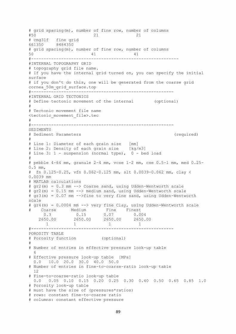
89
# grid spacing(m), number of fine row, number of columns
#50 21 21
# cmg31f fine grid
661350 8484350
# grid spacing(m), number of fine row, number of columns
50 41 41
#-----------------------------------------------------------
#INTERNAL TOPOGRAPHY GRID
# topography grid file name.
# If you have the internal grid turned on, you can specify the initial
surface
# if you don't do this, one will be generated from the coarse grid
cornea_50m_grid_surface.top
#---------------------------------------------------------
#INTERNAL GRID TECTONICS
# Define tectonic movement of the internal (optional)
#
# Tectonic movement file name
<tectonic_movement_file>.tec
#
#---------------------------------------------------------
SEDIMENTS
# Sediment Parameters (required)
#
# Line 1: Diameter of each grain size [mm]
# Line 2: Density of each grain size [kg/m3]
# Line 3: 1 - suspension (normal type), 0 - bed load
#
# pebble 4-64 mm, granule 2-4 mm, vcse 1-2 mm, cse 0.5-1 mm, med 0.25-
0.5 mm,
# fn 0.125-0.25, vfn 0.062-0.125 mm, slt 0.0039-0.062 mm, clay <
0.0039 mm
# MATLAB calculations
# gr2(m) = 0.3 mm --> Coarse sand, using Udden-Wentworth scale
# gr2(m) = 0.15 mm --> medium sand, using Udden-Wentworth scale
# gr3(m) = 0.07 mm -->fine to very fine sand, using Udden-Wentworth
scale
# gr4(m) = 0.0004 mm --> very fine Clay, using Udden-Wentworth scale
# Coarse Medium Fine Finest
0.3 0.15 0.07 0.004
2650.00 2650.00 2650.00 2650.00
1 1 1 1
#---------------------------------------------------------
POROSITY TABLE
# Porosity function (optional)
#
# Number of entries in effective pressure look-up table
6
# Effective pressure look-up table [MPa]
0.0 10.0 20.0 30.0 40.0 50.0
# Number of entries in fine-to-coarse-ratio look-up table
12
# Fine-to-coarse-ratio look-up table
0.0 0.05 0.10 0.15 0.20 0.25 0.30 0.40 0.50 0.65 0.85 1.0
# Porosity look-up table
# must have the size of (pressures*ratios)
# rows: constant fine-to-coarse ratio
# columns: constant effective pressure

90
0.39 0.36 0.35 0.34 0.33 0.32
0.36 0.33 0.31 0.30 0.295 0.29
0.34 0.31 0.28 0.27 0.26 0.25
0.335 0.28 0.23 0.22 0.21 0.20
0.35 0.25 0.21 0.19 0.18 0.17
0.36 0.26 0.20 0.18 0.16 0.14
0.39 0.27 0.21 0.17 0.15 0.13
0.43 0.31 0.24 0.18 0.16 0.12
0.48 0.34 0.27 0.22 0.18 0.14
0.53 0.39 0.31 0.24 0.21 0.17
0.58 0.44 0.35 0.27 0.22 0.19
0.61 0.27 0.17 0.12 0.10 0.09
*
# Porosity table one row for each carbonate and organic
.50 .30 .20 .19 .18 .17
.35 .25 .21 .19 .18 .17
.60 .50 .40 .30 .20 .20
.20 .16 .13 .10 .05 .05
#
#
# Linear weighting coefficients for 4 grain sizes:
# r=Sum(h*w)/Sum(h)
# r fine-to-coarse ratio
# h thickness of individual grain size
# w linear weighting coefficient of individual grain size
# 4 coefficients(one for each siliciclastic grain):
0.0 0.0 1.0 1.0
#----------------------------------------------------------------------
--------------
SOURCES
#
# Definition of sources that are constant throughout the experiment
(required)
# One line per source, entries are:
# Source location (x,y) [m]
# Velocity at source (vx,vy) [m/sec]
# Discharge rate (Q) [m3/sec]
# Sediment concentration (c) [kg/m3]
# Sediment composition (C coarse, [%]
# M medium,
# F fine,
# FF finest)
#
#ID# t1 t2 x y vx vy Q c
%C %M %F %FF
1 -112000000 -56000000 684350 8478250 -0.20 -0.20 5.0
0.2 5 25 35 35
2 -112000000 -56000000 678350 8477250 -0.24 -0.20 5.0
0.2 5 25 35 35
3 -112000000 -56000000 666850 8473250 -0.24 -0.20 5.0
0.2 5 25 35 35
#
4 -120000000 -112000000 667850 8490250 -0.14 -0.14 2.0
0.1 10 25 30 35
5 -120000000 -112000000 659350 8485850 -0.14 0.14 2.0
0.1 5 25 35 35
6 -120000000 -112000000 684850 8477350 0.24 -0.24 2.0
0.1 5 25 35 35

91
*
######################################################################
# Additional module parameters (modules will not run if not included)
##################################################################
#----------------------------------------------------------
SOURCE HEIGHTS
# list ends in '*'
# flow types 0=normal 1=turbidite 2=debris flow
# for debris flows the concentration must be high enough, otherwise
will
# transition to a turbidite (default transition at 60 kg/m3)
#
# source ID# flow height(m) flow type
1 5.0 0
2 10.0 0
3 10.0 0
#
4 5.0 0
5 5.0 0
6 5.0 0
*
#--------------------------------------------------------
WELL LOCATIONS
# locations in meters from Sedsim-grid origin (draws them in sedview)
# X Y
# well name
#
684350 8478350 s1-NW
678350 8477350 s2-wnw
666850 8473350 s3-wnw
667850 8490250 s4-sw
659350 8485850 s5-nw
684850 8477350 s6-se
#
# 659074 8479373 source_1
# 666009 8479868 source_2
# 659569 8486791 source_3
#
662779 8489711 Capsule-1
661217 8485273 Cornea-1
661537 8484924 Cornea-1B
660149 8486497 Cornea-2 checked on WCR
661603 8485159 Cornea-3
657885 8481473 Cornea_South-1
658105 8481252 Cornea_South-2
# 672382 8492083 Focus-1
663768 8488852 Hammer-1
# 663550 8494385 Londonderry-1
# 668441 8492028 Macula-1
668665 8480984 Sparkle-1
667099 8493358 Stirrup-1
# 672298 8497941 Tear-1
#
# 654850 8472850 SW_Corner main 500 m grid
660850 8484350 finegridsw
661850 8485350 finegridne
#
* end of well data

92
#-------------------------------------------------------------------
PARAMETRIC SAMPLING INTERVAL
# (optional)
#
# This should be seen in relation to temporal resolution - ie. think
aliasing
# Sampling interval for sea-level, rainfall and tectonics [y]
100000
#-----------------------------------------------------------
CARBONATES AND ORGANICS
# Parameters for calculating carbonate development (optional)
# (It is strongly recomended that waves are turned on with this module)
# calling interval (years)
100
# carb/org grain size diameter (one for each grain) after comminution
0.3 0.3 0.1 0.1
# carb grain density (one for each grain)
2760.00 2250.00 1800.0 1800.0
# temperature and salinity file (this is a list of year, sea surface
temperature[degrees C] and salinity [ppm])
# to let Sedsim interpolate between unknown values set them to -99
(warning: first value must always be defined)
# eg 2005 27.0 30000
# 2005.2 27.2 -99
# 2005.7 30.0 30250 etc.
# This line is ignored if TEMPERATURE GRID is used
#
Browse_SST_85Ma-0Ma.tmprt
#
#--------------------------------------------------------
SEDIMENT TRANSPORT PARAMETERS
# Limiting factors for sediment transport (optional)
#
# Sedimentation time step factor (sedimentation time step =
# flow time step * sedimentation time step factor)
# Maximum depth of fluid elements [m]
# Minimum velocity of fluid elements [m/s]
# Minimum ratio of sediment load fluid element to average sediment
# load at source [kg/m3]
# Basement hardness factor
1.0e4 10.0 0.05 0.10 1.0E2
#
#--------------------------------------------------------------
SEA LEVEL
# Define sea level curve (optional)
#
# Sea level curve file
#
Haq_plus_dnag.sl
#
#
#--------------------------------------------------------------
#
COMPACTION
# Enable compaction module (optional)
# Enter depthe of post depositional burial by
# Sediment Water
100 83

93
#
#----------------------------------------------------------------------
--
# *** End of input file ***

94
Appendix F: Sedsim Output File (one trace example) in .csv Format
%col row x y simulated_yrsage gr1(m) gr2(m) gr3(m) gr4(m) gr5(m) gr6(m) gr7(m) gr8(m) poro xpos ypos bottom(m) top(m)
1 1 660850 8484350 8500000 -111500000 1.05202 10.837 9.1575 13.6874 0 0 0 0 0.325 0 0 -819.17 -784.436
1 1 660850 8484350 9000000 -111000000 0 0.036596 5.9165 12.119 0 0 0 0 0.193 0 0 -784.436 -766.364
1 1 660850 8484350 16500000 -103500000 0 0 5.7663 0.98595 0 0 0 0 0.192 0 0 -766.364 -759.612
1 1 660850 8484350 19500000 -100500000 0 0 16.686 0.10764 0 0 0 0 0.196 0 0 -759.612 -742.818
1 1 660850 8484350 20500000 -99500000 0 0.14672 15.589 8.4919 0 0 0 0 0.209 0 0 -742.818 -718.59
1 1 660850 8484350 24000000 -96000000 0 0.43751 1.2374 41.087 0 0 0 0 0.224 0 0 -718.59 -675.829
1 1 660850 8484350 25000000 -95000000 2.7412 22.002 6.4044 0 0 0 0 0 0.23 0 0 -675.829 -644.681
1 1 660850 8484350 25500000 -94500000 0.076932 0 0.39199 0 0 0 0 0 0.391 0 0 -644.681 -644.212
1 1 660850 8484350 28000000 -92000000 0.63416 4.3087 0.88055 0 0 0 0 0 0.255 0 0 -644.212 -638.389
1 1 660850 8484350 28500000 -91500000 14.46 3.5187 0 0 0 0 0 0 0.355 0 0 -638.389 -620.41
1 1 660850 8484350 32000000 -88000000 0.003717 0 0 0 0 0 0 0 0.355 0 0 -620.41 -620.406
1 1 660850 8484350 32500000 -87500000 0.93643 0 0 0 0 0 0 0 0.356 0 0 -620.406 -619.47
1 1 660850 8484350 34000000 -86000000 1.1143 0 0 0 0 0 0 0 0.356 0 0 -619.47 -618.355
1 1 660850 8484350 58500000 -61500000 0 0 0 0 0 1.554 0 0 0.232 0 0 -618.355 -616.801
1 1 660850 8484350 59000000 -61000000 0 0 0 0 0 3.1868 0 0 0.233 0 0 -616.801 -613.615
1 1 660850 8484350 59500000 -60500000 0 0 0 0 0 3.1683 0 0 0.233 0 0 -613.615 -610.446
1 1 660850 8484350 60000000 -60000000 0 0 0 0 0 3.1878 0 0 0.233 0 0 -610.446 -607.259
1 1 660850 8484350 60500000 -59500000 0 0 0 0 0 3.1885 0 0 0.233 0 0 -607.259 -604.07
1 1 660850 8484350 61000000 -59000000 0 0 0 0 0 3.1884 0 0 0.234 0 0 -604.07 -600.882
1 1 660850 8484350 61500000 -58500000 0 0 0 0 0 3.1901 0 0 0.234 0 0 -600.882 -597.692
1 1 660850 8484350 62000000 -58000000 0 0 0 0 0 3.1908 0 0 0.234 0 0 -597.692 -594.501
1 1 660850 8484350 62500000 -57500000 0 0 0 0 0 3.1914 0 0 0.234 0 0 -594.501 -591.309
1 1 660850 8484350 63000000 -57000000 0 0 0 0 0 3.1703 0 0 0.235 0 0 -591.309 -588.139
1 1 660850 8484350 63500000 -56500000 0 0 0 0 0 3.1824 0 0 0.235 0 0 -588.139 -584.957
1 1 660850 8484350 64000000 -56000000 0 0 0 0 0 3.1847 0 0 0.235 0 0 -584.957 -581.772
1 1 660850 8484350 64500000 -55500000 0 0 0 0 0 15.807 0 0 0.236 0 0 -581.772 -565.965
1 1 660850 8484350 65000000 -55000000 0 0 0 0 0 16.075 0 0 0.238 0 0 -565.965 -549.89
1 1 660850 8484350 65500000 -54500000 0 0 0 0 0 16.52 0 0 0.239 0 0 -549.89 -533.37
1 1 660850 8484350 66000000 -54000000 0 0 0 0 0 17.688 0 0 0.24 0 0 -533.37 -515.682
1 1 660850 8484350 66500000 -53500000 0 0 0 0 0 18.399 0 0 0.242 0 0 -515.682 -497.283
1 1 660850 8484350 67000000 -53000000 0 0 0 0 0 18.421 0 0 0.243 0 0 -497.283 -478.862
1 1 660850 8484350 67500000 -52500000 0 0 0 0 0 18.443 0 0 0.245 0 0 -478.862 -460.419
1 1 660850 8484350 68000000 -52000000 0 0 0 0 0 18.465 0 0 0.246 0 0 -460.419 -441.954
1 1 660850 8484350 68500000 -51500000 0 0 0 0 0 18.487 0 0 0.248 0 0 -441.954 -423.467
1 1 660850 8484350 69000000 -51000000 0 0 0 0 0 18.509 0 0 0.249 0 0 -423.467 -404.958
1 1 660850 8484350 69500000 -50500000 0 0 0 0 0 13.863 0 0 0.251 0 0 -404.958 -391.095
1 1 660850 8484350 70000000 -50000000 0 0 0 0 0 6.4945 0 0 0.253 0 0 -391.095 -384.6
1 1 660850 8484350 70500000 -49500000 0 0 0 0 0 4.6427 0 0 0.254 0 0 -384.6 -379.958
1 1 660850 8484350 71000000 -49000000 0 0 0 0 0 3.5972 0 0 0.254 0 0 -379.958 -376.361
1 1 660850 8484350 71500000 -48500000 0 0 0 0 0 5.1142 0 0 0.255 0 0 -376.361 -371.246
1 1 660850 8484350 72000000 -48000000 0 0 0 0 0 6.9818 0 0 0.257 0 0 -371.246 -364.265
1 1 660850 8484350 72500000 -47500000 0 0 0 0 0 16.904 0 0 0.26 0 0 -364.265 -347.361
1 1 660850 8484350 73000000 -47000000 0 0 0 0 0 18.724 0 0 0.264 0 0 -347.361 -328.637
1 1 660850 8484350 73500000 -46500000 0 0 0 0 0 18.78 0 0 0.268 0 0 -328.637 -309.857
1 1 660850 8484350 74000000 -46000000 0 0 0 0 0 18.836 0 0 0.271 0 0 -309.857 -291.021
1 1 660850 8484350 74500000 -45500000 0 0 0 0 0 18.892 0 0 0.275 0 0 -291.021 -272.129
1 1 660850 8484350 75000000 -45000000 0 0 0 0 0 18.398 0 0 0.279 0 0 -272.129 -253.731
1 1 660850 8484350 75500000 -44500000 0 0 0 0 0 15.229 0 0 0.282 0 0 -253.731 -238.502
1 1 660850 8484350 76000000 -44000000 0 0 0 0 0 12.024 0 0 0.284 0 0 -238.502 -226.478
1 1 660850 8484350 76500000 -43500000 0 0 0 0 0 7.5317 0 0 0.286 0 0 -226.478 -218.946
1 1 660850 8484350 77000000 -43000000 0 0 0 0 0 7.024 0 0 0.287 0 0 -218.946 -211.922
1 1 660850 8484350 77500000 -42500000 0 0 0 0 0 4.3771 0 0 0.288 0 0 -211.922 -207.545
1 1 660850 8484350 80500000 -39500000 0 0 0 0 0 0.59654 0 0 0.288 0 0 -207.545 -206.948
1 1 660850 8484350 81500000 -38500000 0 0 0 0 0 0.000738 0 0 0.288 0 0 -206.948 -206.948
1 1 660850 8484350 82500000 -37500000 0 0 0 0 0 2.3312 0 0 0.289 0 0 -206.948 -204.616
1 1 660850 8484350 83000000 -37000000 0 0 0 0 0 3.2431 0 0 0.289 0 0 -204.616 -201.373
1 1 660850 8484350 83500000 -36500000 0 0 0 0 0 4.6796 0 0 0.29 0 0 -201.373 -196.694
1 1 660850 8484350 84000000 -36000000 0 0 0 0 0 2.277 0 0 0.291 0 0 -196.694 -194.417
1 1 660850 8484350 84500000 -35500000 0 0 0 0 0 0.001427 0 0 0.291 0 0 -194.417 -194.415
1 1 660850 8484350 1.01E+08 -19000000 0 0 0 0 0 0.11962 0 0 0.291 0 0 -194.415 -194.296
1 1 660850 8484350 1.02E+08 -18500000 0 0 0 0 0 2.8701 0 0 0.291 0 0 -194.296 -191.425
1 1 660850 8484350 1.02E+08 -18000000 0 0 0 0 0 6.2241 0 0 0.293 0 0 -191.425 -185.201
1 1 660850 8484350 1.03E+08 -17500000 0 0 0 0 0 9.5893 0 0 0.295 0 0 -185.201 -175.612
1 1 660850 8484350 1.03E+08 -17000000 0 0 0 0 0 12.972 0 0 0.297 0 0 -175.612 -162.64
1 1 660850 8484350 1.04E+08 -16500000 0 0 0 0 0 14.498 0 0 0.3 0 0 -162.64 -148.142
1 1 660850 8484350 1.04E+08 -16000000 0 0 0 0 0 6.8187 0 0 0.301 0 0 -148.142 -141.323
1 1 660850 8484350 1.05E+08 -15500000 0 0 0 0 0 17.677 0 0 0.305 0 0 -141.323 -123.646
1 1 660850 8484350 1.05E+08 -15000000 0 0 0 0 0 7.4917 0 0 0.306 0 0 -123.646 -116.155
1 1 660850 8484350 1.06E+08 -14500000 0 0 0 0 0 14.353 0 0 0.309 0 0 -116.155 -101.802
1 1 660850 8484350 1.06E+08 -14000000 0 0 0 0 0 12.748 0 0 0.312 0 0 -101.802 -89.054
1 1 660850 8484350 1.07E+08 -13500000 0 0 0 0 0 5.5517 0 0 0.313 0 0 -89.054 -83.502
1 1 660850 8484350 1.07E+08 -13000000 0 0 0 0 0 2.2145 0 0 0.313 0 0 -83.502 -81.287
1 1 660850 8484350 1.08E+08 -12500000 0 0 0 0 0 2.8428 0 0 0.314 0 0 -81.287 -78.445
1 1 660850 8484350 1.2E+08 0 0 0 0 0 1.5442 1.4832 0 0 0.373 0 0 -78.445 -75.417

95
Appendix G: Geoscience Australia Copyright Statement

96
Appendix H: Geoscience Australia Copyright Permission

97
Appendix I: Cedric Griffiths Copyright Permission

98
Appendix J: SegyMAT Copyright Statement

99
Appendix K: Depositional Environment Description