Integration and Transition:

Scenarios for Location of Production and Trade in Europe*

Rikard Forslid University of Stockholm and CEPR

Jan I. Haaland

Norwegian School of Economics and Business Administration and CEPR

Karen Helene M. Knarvik Norwegian School of Economics and Business Administration and CEPR

Ottar Mæstad

Foundation for Research in Economics and Business Administration ABSTRACT Applying a newly developed CGE-model, we present scenarios for the future economic geography of Europe. The model divides the world into ten regions, of which five are European, and there are 14 industries, of which 12 are imperfectly competitive. With a complete input-output structure, the model captures comparative advantage mechanisms as well as intra-industry trade and “new economic geography” agglomeration forces. The simulations focus on the consequences of successful transformation in Eastern Europe. The results indicate that transformation and European integration are of great importance for Eastern Europe, while the overall effects for other European regions are small. Individual sectors in EU, such as Textiles and Transport Equipment, are however in some cases strongly affected.

Bergen, March 2001

* Thanks to Richard Baldwin and Victor D. Norman for very valuable discussions and comments, and to Joseph Francois for providing data on demand elasticities. We also thank two anonymous referees for valuable comments. This research has been financed by the Research Council of Norway grants nos. 40050/230 and 124559/510. The work was carried out while Forslid visited Bergen under a TMR grant from the European Commission (TMR-programme FDI MC).

1

1. Introduction

The economic integration of the Eastern European countries is often identified as one

of the main challenges for the EU. Clearly a successful integration of these states

would mean a major improvement for Europe as a whole not only in economic terms,

but also in terms of enhanced security. A revived Eastern Europe means new export

markets but, of course, also enhanced competition, for instance, in the form of low

wage manufacturing imports to the EU.

The purpose of this paper is to assess, through model simulations, the long-

term production and trade effects of an Eastern European transformation. While both

economic integration and Eastern European transformation have been studied before1,

we believe our analysis has something to add. We apply a newly developed model

that incorporates several features that have not been implemented in CGE-models

before, and has a regional structure that allows us to identify effects for various parts

of Europe. In particular, we calibrate the model on actual, region-specific, complete

input-output matrices. By modelling all intra- and inter-industry linkages in a setting

with imperfect competition and trade costs, we are able to capture important

agglomeration forces. Furthermore, we specify several scenarios that differ from

previous studies. In particular, for Eastern European transformation we include

productivity improvements and a lower risk premium as well as the more common

experiment of closer market integration.

The model is based on both traditional trade theory and more recent theory of

international trade and economic geography. In this way it captures comparative

advantage as well as agglomeration effects of structural changes or policy events. Five

1 European integration has been studied in many model-based analyses, e.g. Gasiorek, Smith and Venables (1991, 1992), Haaland and Norman (1992, 1995), Baldwin, Forslid and Haaland (1996), Allen, Gasiorek and Smith (1998), Keuschnigg and Kohler (1996). For studies of Eastern European transformation and eastern enlargement of the EU, see e.g. Baldwin, Francois and Portes (1997) or

2

of the ten regions in the model are European ones. Hence, the model should be

suitable for analysing regional development in Europe – where phenomena like

agglomeration effects and the centre-periphery dimension have been emphasised in

the theoretical and applied literature, but so far not been implemented in a full-scale

general equilibrium model calibrated on actual data.

Eastern Europe has experienced a number of very significant changes since

1989, on both the political and the economic arena. However, we have not yet seen

the long-term effects of the economic reforms. What we have observed so far in most

of the countries, is more of the short-term adjustment problems and less of the long-

term possibilities. This paper analyses possible long-run outcomes such as produc-

tivity growth and investment.

In all experiments we study stylised characteristics rather than trying to assess

the exact nature or magnitude of the exogenous changes. Hence, the results should be

read as “what – if” type of experiments not as complete scenarios for the future

production and trade patterns of Eastern Europe and its trading partners.2 Moreover,

the absolute magnitudes of the effects obtained in this type of simulations must be

treated with caution. However, in a qualitative sense we expect the results to be much

more robust.

In the next section the model is presented, while section 3 reviews some

important aspects of the benchmark data. Section 4 presents the simulation results,

while conclusions are given in the final section.

Keuschnigg and Kohler (1998). 2 In Forslid et al (1999a) the approach is discussed in more detail.

3

2. The model

The model has ten regions. In each region there are fourteen production sectors; the

regions and sectors are listed in Table 1 below. There are three primary factors of

production – capital, skilled labour and unskilled labour; these are mobile between

industries within a region, but immobile between regions.3 The supply of the two

types of labour is exogenously given; for capital the supply is endogenously

determined by the condition that the return to capital should equal the steady-state

level, which is calculated in the benchmark case. The factor demand comes from the

fourteen producing sectors. In addition to the three sectorally mobile factors, two of

the sectors – energy and agriculture –use sector-specific natural resources. Hence,

these two sectors show decreasing returns to scale with respect to the mobile factors.

Energy and agriculture are modelled as perfectly competitive and with free trade4.

The remaining twelve sectors are all modelled with increasing returns to scale,

imperfect competition and product differentiation. For the ten manufacturing sectors

in the model, there are trade flows between all regions, but trade costs hamper trade.

The two imperfectly competitive services sectors in the model are assumed to be non-

traded. Although trade in services is not negligible in reality, it is clear from the

benchmark data that a very large share of the output from these sectors is sold in

domestic markets.

3 The regional immobility assumption is consistent with the empirical observation that the return to capital differs widely between countries. See Ménil (1999) for evidence related to the European capital market. 4 The assumptions of perfect competition and free trade for these two sectors are not realistic ones; however, since the emphasis of the model is on manufacturing, we have kept the resource-based sectors as simple as possible. With perfect competition and homogenous products, the model will only deter-mine the net trade position of a region, and that is why we do not include trade policies for these goods. The model includes production subsidies in agriculture and energy; however, in the scenarios presented in this paper, these policies are kept unaltered. These policies may still give rise to second best effects in our model simulations.

4

Table 1: Regions and sectors in the model Regions Trade manufactures (imperf. comp., IRS, diff. prod.) Europe Central (EuropeC) Austria, Denmark, Germany, Switzerland

Textiles Leather

Europe North (EuropeN) Finland, Iceland, Norway, Sweden

Wood and pulp products Metals

Europe South (EuropeS) Greece, Italy, Portugal, Spain

Minerals Chemicals

Europe West (EuropeW) BeNeLux, Ireland, France, UK

Food products Transport equipment

Europe East (Europe E) Bulgaria, Hungary, Czeck. Rep., Poland, Romania, Slovakia, Slovenia

Machinery and equipment Other manufacturing

Former Soviet Union (FormSov) Former Soviet Republics including Estonia, Lithuania, Latvia

Non-traded services (imperf. comp., IRS, diff. prod.) Public services Private services

China and South Asia (CSA) China, India, Bangladesh, Bhutan, Maldives, Nepal, Pakistan, Sri Lanka

Traded resource intensive industries (perf comp., free trade)Agriculture

South East Asia (SEA) South East Asia including Japan

Energy goods

USA and Canada (USACAN) Rest of the World (ROW)

One important feature of the model is the input-output linkages between sectors.

There is a complete input-output system, and together with trade costs and imperfect

competition this creates a force for agglomeration through backward and forward

linkages (see e.g. Venables, 1996).5 The data reveals a clear pattern of these linkages:

for most industries inputs from own industry dominate, with inputs from the services

industries as number two. Hence, the non-traded nature of the services industries as

well as the trade costs for manufactures are potential sources of agglomeration in this

model. We calibrate parameters of the cost function using actual region and industry

specific input-output matrices. Most previous models (e.g. Norman and Haaland,

1992) use a common CES-composit of differentiated goods as intermediate input,

which implies that differences at the industry level are not taken into account. This is

a strong assumption when analysing agglomeration forces. For instance, a region with

a large textile industry may not provide strong linkages to firms in the steel industry.

5 In the new economic geography literature two major sources of agglomeration have been emphasized: Linkages between mobile firms (as in Venables, 1996) and factor mobility (as in Krugman, 1991). Here

5

Thus, the use of region and industry specific input-output data is important as means

of capturing real world agglomeration forces.

Basic model equations

We here display some basic model equations to illustrate how specific features of the

model work; a complete description is found in Forslid et al (1999a) 6.

Consumers in region m have Cobb-Douglas preferences over a set of all

goods (AG), implying that they will spend a fixed share of their income on each good:

im

imimim P

YC α= AGi ∈ (1.)

For perfectly competitive goods prices are world market prices given by world market

clearing conditions for the respective goods. One of these goods is chosen as

numeraire. As for imperfectly competitive, differentiated goods (the set I), the price

level for good i (Pim) is an index of the prices of each variety of the good sold in

market m (PIijm). The calibrated demand parameter for each of the Nij varieties of

good i from country j sold in market m, is aijm.

( ) ii

R

jijmijmijim PIaNP

σσ

−

=

−

⎟⎟⎠

⎞⎜⎜⎝

⎛= ∑

11

1

1 Ii ∈ (2.)

For non-traded, differentiated goods aijm=0 for all m≠j, since by assumption only

domestically produced varieties are consumed. σi is the elasticity of substitution

between various varieties of good i.

we focus on the former of these. 6 The model builds on Haaland and Norman (1992), but with significant differences. The regional set-up differs, and so does the input-output structure. Hence the present model is more suitable for economic geography issues. The model has similarities with a few other models, like e.g. the one applied in Baldwin et al (1997) but, again, the regional as well as the input-output structure is richer in the present model. The CGE-model sketched in Gasiorek and Venables (1998) focuses on the effects of transport improvements on industrial location and real income. Those simulations, however, are based on made up data.

6

The imperfectly competitive sectors are characterised by monopolistic

competition á la Dixit and Stiglitz (1977) with free entry and zero profits. Producer

prices (PPI) of individual varieties are given as a mark-up over firms’ marginal costs

(MC):

1

iij ij

i

PPI MCσσ

=−

Ii ∈ (3.)

while consumer prices (PIijm) for the traded goods are subject to trade costs, Tijm.7

( )1ijm ij ijmPI PPI T= + ITGi ∈ (4.)

where ITG is the set of imperfectly competitive traded goods. Demand for each

variety of good i in market m may now be derived as:

imijm

imijmijm C

PIP

aXiσ

⎟⎟⎠

⎞⎜⎜⎝

⎛= ITGi ∈ (5.)

Prices and demand for non-traded differentiated goods are derived in the same way as

for traded goods, but with no need to distinguish between producer and consumer

prices since there is only domestic consumption of these goods.

The price index for differentiated intermediate goods (Qhm) is industry

specific by purchasing industry (h) and region (m). The industry uses all goods as

inputs, weighting the aggregate price of each good by the parameter gihm. The

parameter is calibrated from the use of good i as intermediate input in the production

of industry h in country m.

( ) sq

Ii

sqimihmhm PgQ

−

∈∀

−⎟⎟⎠

⎞⎜⎜⎝

⎛= ∑

11

1 AGh ∈∀ (6.)

7 T includes trade costs of three types: export taxes (EXTAX) levied by the exporting country, transport costs (TRANS), and tariff equivalents of import barriers (TAREQ) set up by the importing country. The transport costs are of the iceberg type, while export taxes and import tariffs are transfers (to the

7

where sq is the elasticity of substitution among imperfectly competitive goods used as

intermediates. The price indices for perfectly competitive goods (the set PC) as

intermediates are constructed in the same way, where the market price for perfectly

competitive goods is denoted by PPC.

( ) sq

PCi

sqiihmhm PPCgQPC

−

∈∀

−⎟⎟⎠

⎞⎜⎜⎝

⎛= ∑

11

1 AGh ∈∀ (7.)

PVij is a price aggregate for all primary factors used in the production in sector i in

region j. The use of each individual factor is industry and country specific and given

by the parameter β.

i

isK

k

sjkijkij WPV

−

=

−⎟⎟

⎠

⎞

⎜⎜

⎝

⎛= ∑

11

1

1β AGi ∈ (8.)

Finally, the marginal cost for industry i in country j is specified as a nested CES-

function, with primary inputs, differentiated intermediates, and homogenous

intermediates in one second-level nest each, and with Stop as the elasticity of

substitution between the nests at the top level. Using the price indices above, the

marginal cost function can we written

( ) ( ) ( ) 11

1 1 1 Stoptop top top ii i iS S S

ij ij ij ij ij ij ijMC BV PV BZ Q BZPC QPC−− − −⎡ ⎤= + +⎢ ⎥⎣ ⎦

, (9.)

where BVij, BZij, and BZPCij are all calibrated parameters. From (9), using (6) – (8)

and market clearing conditions for each good, we find the demand for primary factors

and intermediate goods from each sector. Together with supply conditions, these

form the general equilibrium system. As the imperfectly competitive sectors are

representative consumer). T is constructed according to: 1+ ( )( )( )1 1 1ijm ijm ijm ijmT EXTAX TRANS TAREQ= + + + ITGi ∈

8

characterised by monopolistic competition and zero profits, the scale of each firm is

fixed, and any output expansion is entirely reflected through an increase in the

number of firms (varieties) in the respective sector.

The use of intermediates from own as well as other industries implies

externalities through the existence of inter- and intra-industry cost and demand

linkages. These effects can be seen from the presence of the second and third term in

(9) and from (6). The parameters in (9) are calibrated using actual region and industry

specific input-output tables. For instance, in (9), a high BZij for a particular industry i

implies that manufacturing inputs are important, while a high giim in (6) implies that

inputs from your own industry are important. In this case, given the existence of trade

costs, your production costs are reduced if you are located in a region with a high

concentration of firms in your own industry. This dependence on intermediate inputs

from other firms is often referred to as the supply (or forward) link (se e.g. Venables

1996). In the same fashion the parameters of (9) (by the use of Shepard´s lemma)

determine which sectors and regions are important buyers of your product as

intermediate input. Because of the trade costs, you would increase your operating

profits by locating in a region with a high demand for your product. This comprises

the demand (or backward) link. The presence of these linkages implies pecuniary

externalities. Firms located in a region with a large number of buyers and suppliers of

important intermediates, will be relatively more competitive ceteris paribus.

Because our model has endogenous capital stocks, there is an additional

agglomeration force. More capital expands output via firm entry, which entails an

increased number of varieties. Consequently, the price indices for the imperfectly

competitive goods decline, which feeds back on investment and makes yet more

capital investments profitable – an instance of cumulative causation.

9

Agglomeration forces do not directly affect the perfectly competitive sectors.

These sectors, however, expand or contract as a consequence of competition for

factors with the other sectors. The decreasing returns to scale in these sectors (due to a

specific factor) act to dampen the expansion of the ITG sectors.

Data

The model is calibrated on actual data for1992, which is used as benchmark year.

Data sources for input-output tables, trade flows and factor shares are EUROSTAT

(EU input-output tables), GTAP (Global Trade Analysis Project) version 3 database

and NBER World Trade Flows (see Feenstra et al, 1997). A detailed description of

data, data sources, and how the benchmark data set was constructed, can be found in

Forslid et al (1999a) or obtained from the authors upon request. Forslid et al (1999a)

also provide a descriptive analysis of the data material, focusing on the distribution of

production across regions, trade flows and trade volume, differences in technology

and factor use across industries. Our data on economies of scale estimates have been

based on Pratten (1988). Transport costs and data on trade barriers are from GTAP

versions 3 and 4.

3. The benchmark case

In this section we briefly review some key characteristics of production and trade that

are important when it comes to understanding the scenarios we later construct.

10

Table 2: Key characteristics – Base case 1992 The region's share (measured in percent) of World World manufacturing World production of GDP exports imports energy agriculture EuropeW 12.09 17.65 17.70 12.52 8.71 EuropeC 11.75 18.50 17.88 7.09 3.54 EuropeS 8.27 8.84 8.80 7.34 6.05 EuropeN 1.96 3.51 3.45 2.16 1.69 EuropeE 0.89 2.06 2.78 1.53 2.57 FormSOV 2.21 0.78 0.78 3.79 2.11 CSAsia 3.17 4.39 4.37 3.12 17.07 SEAsia 20.27 20.80 20.80 12.94 18.31 USACAN 27.71 15.74 15.75 20.46 16.07 RestofW 11.67 7.73 7.69 29.05 23.87

Table 2 shows some key characteristics. First, it is important to notice the significant

differences in size between the regions. In particular when we analyse the effects of

successful transformation in Eastern Europe, it should be remembered that in

economic terms this region is very small. Secondly, trade is relatively more important

for the European regions than for the other regions8; in part this reflects the close

integration within Europe, but it should be observed that trade flows are relatively

important for Europe East as well. Finally, the table shows that the regions differ

significantly when it comes to relative importance of the resource-based industries. In

particular, in Europe East, Former Soviet Union, China and South Asia, and the rest

of the world, the shares of energy and/or agriculture production are higher than these

regions’ overall shares of global GDP.

Next we focus on manufacturing. Table 3 shows the pattern of specialisation

as measured by the Hoover localisation quotient; for each industry in a region, the

number shows the region’s share of global production (measured by value added) in

this industry relative to the region’s overall share of manufacturing value added.

8 The table only reports trade between the regions; in addition there may be significant trade flows between the countries within each region.

11

Hence, a number greater than one indicates that this industry is of more than average

importance for the region.

The pattern of specialisation is, to a large extent, as we should expect. The

big, advanced regions like Europe Central and West, USA and Canada, and South

East Asia specialise in skill-intensive products (Transport equipment, Machinery),

while poorer regions like Europe East, China and South Asia, and also Europe South

specialise in labour intensive products (Textiles and Leather).

Table 3: The pattern of manufacturing specialisation Share of the industry’s value added relative to share of total manufacturing value added EuropeW EuropeC EuropeS EuropeN EuropeE Form

SOV CSAsia SEAsia USA&

CAN Rest of World

Textiles 0.78 0.58 1.61 0.53 1.59 0.73 2.51 0.86 0.78 1.71 Leather 0.88 0.56 3.15 0.72 2.75 0.22 2.17 0.86 0.34 1.68 WoodProd 1.06 0.91 0.87 1.63 1.03 1.12 0.48 0.84 1.25 0.91 Metals 0.96 1.05 1.15 1.19 1.16 1.04 0.82 1.07 0.90 0.95 Minerals 0.92 0.70 1.17 1.06 1.57 1.52 1.87 0.92 0.74 1.67 Chemical 1.06 0.98 0.92 0.83 0.89 0.88 0.84 0.97 1.06 1.05 FoodProd 1.08 0.81 1.13 0.89 1.31 1.13 0.92 0.94 0.84 1.57 TransEq 1.15 1.32 0.84 0.84 0.47 1.09 0.38 0.87 1.23 0.61 Machines 0.95 1.18 0.74 1.01 0.60 0.90 0.70 1.22 1.10 0.44 OtherMan 0.96 1.48 0.54 0.64 0.91 0.73 3.74 0.95 0.66 1.01

Europe East is also fairly specialised in energy- and natural resource-intensive

industries, like Metals, Minerals and Food products. A similar pattern appears for

Europe North, with specialisation in Wood Products and Metals.

The geographical pattern of trade is reviewed in Table 4, which shows the

geographical distribution of manufacturing sales from each region. A couple of

observations are due. First, the home market dominance is very clear in all regions,

but less so in Europe than in the other regions. The explanation for this is obvious;

Europe is split into five regions with close ties among them. Second, geographical

closeness seems to matter; Europe Central typically has strong trade links to the other

European regions. In Asia, South East Asia is the most important trading partner for

12

China and South Asia. Thirdly, the strong trade links between Europe East and

Europe Central should be noticed; Europe Central is by far the most important market

for exports from Europe East, and it is also the most important supplier of imports to

Europe East.

Table 4: Geographical patterns of manufacturing sales Distribution (in percent) of total sales of manufactures from a region Sales to EuropeW EuropeC EuropeS EuropeN EuropeE Form

SOV CSAsia SEAsia USA&

CAN Rest of World

From EuropeW 69.3 11.2 6.9 1.4 0.5 0.3 0.5 2.5 3.6 3.7EuropeC 11.9 71.3 5.5 1.9 1.4 0.6 0.4 2.4 2.5 1.9EuropeS 8.1 7.0 78.0 0.6 0.6 0.4 0.2 1.3 1.8 2.1EuropeN 8.6 7.9 2.7 73.5 0.5 0.5 0.4 1.8 2.6 1.4EuropeE 3.6 10.5 3.6 1.0 74.8 1.2 0.6 0.9 0.8 3.1FormSOV 0.7 0.9 0.5 0.4 0.5 94.3 1.3 0.7 0.3 0.5CSAsia 1.1 0.9 0.5 0.1 0.1 0.6 82.0 7.2 4.7 2.9SEAsia 1.3 1.2 0.5 0.2 0.1 0.1 1.6 87.5 5.3 2.3USACAN 1.8 0.9 0.5 0.2 0.1 0.1 0.4 3.1 89.4 3.5RestofW 1.4 0.9 0.8 0.1 0.2 0.1 0.5 2.2 4.1 89.8

Trade costs, elasticity of substitution, scale economies, and input-output coefficients

are key parameters in our model, and affect the strength of linkages and cumulative

causation. Note, however, that in a model such as ours with large-group monopolistic

competition and free entry/exit, there is in equilibrium a one-to-one (inverse)

relationship between elasticity of substitution between varieties and scale elasticity.

This is a property we use when characterising the industries. The scale elasticities

used here are based on a ranking of industries according to engineering estimates of

scale economies by Pratten (1988).9 Table 5 shows a summary of trade costs and

returns to scale. It is evident that scale economies are most significant in the sectors

producing Transport equipment, Chemicals, Machinery and Metals. Hence, these are

sectors where market size matters the most; i.e. where firms’ competitiveness depends

on their market access.

9 In the sensitivity testing section below we use mark-up estimates provided by Martins, Scarpetta and

13

The use of intermediates is also a factor determining the location of production

and magnitude of agglomeration forces. The sixth column in Table 5 gives purchases

of intermediates from own sector as share of gross value of output. Supplies from own

sector create a positive feedback – via cost and demand linkages – and make

agglomeration self-reinforcing. From Table 5 we can see that Textiles, Wood

Products, Minerals and Chemicals are industries with an above average use of inputs

from own sector.

Table 5: Summary of trade distortions, scale economies Average Intra

EEA trade costs*)

Trade costs on exports from EuropeE into

EEA*)

Returns to scale**)

Share of inputs from own sector in

total costs***)

Textiles 4.7 29.3 0.06 0.357 Leather and Products 3.7 10.8 0.06 0.192 Wood Products 0.6 6.5 0.12 0.239 Metals 4.5 11.4 0.16 0.259 Minerals 7.0 16.7 0.10 0.272 Chemicals 6.5 20.6 0.24 0.279 Food Products 15.1 46.7 0.08 0.128 Transport Equipment 2.3 9.3 0.26 0.185 Machinery 2.6 6.1 0.20 0.203 Other Manufacturing 3.1 6.3 0.08 0.055 *) Percentage of producer price, averaged over the four EEA regions. **) Percent reduction in average cost (AC) with a one-percent increase in output. ***) Based on Eastern European input-output matrices.

Location of production is moreover affected by comparative advantage, i.e. by

differences in factor endowments and factor intensities. Value added shares and factor

intensities ratios are shown in Table 6. Chemicals, Transport equipment and

Machinery are skill-intensive sectors. Textiles and Leather are intensive in the use of

unskilled labour. Food Products and Minerals are the most capital-intensive

industries, while Transport equipment, Textiles, and Machinery are the least capital-

intensive industries.

Pilat (1996).

14

Table 6: Value added shares (based on Europe East).

Skilled Labour

Unskilled Labour

Capital Skilled/ Unskilled ratio

Labour/ Capital ratio

PubServ 0.476 0.321 0.203 1.483 3.926 PrivServ 0.140 0.436 0.424 0.321 1.358 Textiles 0.085 0.583 0.332 0.146 2.012 Leather 0.081 0.571 0.348 0.142 1.874 WoodProd 0.085 0.561 0.354 0.152 1.825 Metals 0.087 0.534 0.379 0.163 1.639 Minerals 0.077 0.492 0.431 0.157 1.320 Chemical 0.108 0.42 0.472 0.257 1.119 FoodProd 0.073 0.424 0.503 0.172 0.988 TransEq 0.127 0.584 0.289 0.217 2.460 Machines 0.148 0.531 0.321 0.279 2.115 OtherMan 0.073 0.579 0.348 0.126 1.874 Agricult 0.009 0.504 0.145 0.018 3.538 Energy 0.036 0.301 0.405 0.120 0.832

4. Simulation results

The aim of the simulations is to get an impression of the consequences for production,

trade and development should Eastern Europe transform into well-functioning market

economies and become more integrated into the EU.

Apart from trade integration, a “successful transformation” of the Eastern

European economies includes several features. It is a change from the old command

economy to a market system, and it is a change towards freer trade relations and

maybe new trade partners. It includes a restructuring of industry and changes in the

pattern of production and consumption. It implies an improvement in resource

allocation and better investment and employment opportunities and, ultimately,

increased income and welfare. In a general equilibrium model some of these

implications appear as endogenous equilibrium effects, while others must be specified

as exogenous changes. The model cannot capture the transformation from non-market

to market economy endogenously. But it can help us understand what the

consequences may be for production, trade, and welfare under various possible

scenarios.

15

We will look at three “stylised stages” of successful transition. The first case is

one in which we study the consequences of improved productivity in all sectors in the

relevant region. There are a number of reasons why we should expect such

productivity improvements: transformation to market economies implies more

efficient organisation of production, more cost-efficient production and more

competition in goods and factor markets, both within, and between, countries. All of

these changes will lead to more efficient production. In our stylised case we analyse

the general equilibrium consequences of an exogenously given 2.5 and 5 percent

Hick-neutral productivity improvement in all industries in the region in question. In

reality, there will, of course, be differences between industries; some may experience

huge improvements, while for others the scope for improvements is less. Lack of

information about individual industries prevents us from modelling sector-specific

variation.

Our second case focuses on investments. It is widely assumed that successful

transformation would imply a better investment climate in Eastern Europe. While the

combination of low production costs and closeness to the big European markets may

already give high expected rates of returns to investments in Eastern Europe,

uncertainties regarding the general development have so far dampened the actual

willingness to invest. In this scenario we lower the required risk premium for

investments in Europe East, to reflect the improved confidence following a successful

transformation. In the model the aggregate capital stock in a region is determined

from a steady-state condition such that the capital stock will grow until the marginal

rate of return is equal to the steady-state required rate.10 Reduced uncertainties entail

10All economies are assumed to be in steady state in the benchmark case. From a standard neoclassical growth model the steady-state capital stock is determined by parameters of the model such as the subjective rate of time preference. We, thus, calculate the steady-state real return to capital in the benchmark case, and in all experiments the capital stock adjusts until this steady-state return is

16

lower required rate of return, and a higher aggregate capital stock. But where – in

what industries – will investments be undertaken when the overall investment climate

improves? This depends on the relative profitability of various industries, and is one

of the questions our simulation model allows us to address. Note that our model does

not have any transitional dynamics – we do not model the transition whereby foregone

consumption is used to build up the capital stock. This implies that while we can

compare the real income in different steady-states we are not in a position to make a

proper welfare calculation taking into account the present value of forgone

consumption during the capital accumulation phase towards a new steady-state.

Previous analyses of Eastern European transition, in particular Baldwin et al

(1997) and Keuschnigg and Kohler (1998), have focused on market access and EU

enlargement; hence, trade liberalisation has been the key aspect. In our third

simulation exercise, we also analyse the effects of trade liberalisation in the form of

lower tariff equivalents of import barriers. However, to bring forward possible

sectoral differences, we consider an experiment where tariff equivalents between

Eastern Europe and the European Economic Area (EEA) are lowered towards the

(internal) EEA average instead of a uniform reduction in tariff equivalents.11

Economy wide effects

Table 7a shows the real income effects for all the regions for the cases sketched

above. The specific model experiments are: i) 2.5 and 5 percent Hicks-neutral

productivity improvement in all sectors in Eastern Europe (EE); ii) 5 and 10 percent

achieved. See Baldwin et al (1996) for further explanations of this approach. 11 The EEA average tariff equivalent is zero in most industries in our data; five exceptions exist: Textiles, Metals, Chemicals, Food products, and Transport equipment. Of these, Food products in particular, have substantial intra EEA tariff equivalents of 26.5 percent on average. (Note, that total trade costs for intra EEA trade of this type of goods are lower due to the presence of export subsidies.) Our experiment therefore gives a less dramatic effect on this sector than would a flat rate reduction.

17

reduction in the steady-state return to capital EE ; and iii) 10 and 20 percent sector-by-

sector reduction in the gap between Eastern Europe-EEA tariffs and intra-EEA

average tariffs. Note that the range of experiments implicitly also provide a sensitivity

test of the model.

The simulations suggest that the changes are of great importance for Eastern

Europe itself, while the consequences for other regions are minor. This result

corresponds well to the general impression of other studies.12

Table 7a: Real income effects (percent change from base case) Productivity Risk premium Liberalisation 2.5 % 5% -5% -10% 10% 20%

EuropeW 0.02 0.03 0.01 0.02 0.03 0.12 EuropeC -0.06 -0.12 -0.04 -0.08 -0.08 -0.31 EuropeS 0.00 -0.01 -0.01 -0.01 0.00 -0.01 EuropeN -0.03 -0.05 -0.02 -0.04 0.00 -0.01 EuropeE 7.61 15.88 4.81 9.94 2.54 12.38 FormSov 0.00 -0.01 0.00 -0.01 0.00 -0.01 CSAsia -0.06 -0.13 -0.04 -0.08 -0.08 -0.22 SEAsia 0.01 0.01 0.00 0.00 0.01 -0.01 USACAN 0.00 0.00 0.00 0.00 0.00 0.00 RestofW -0.02 -0.04 -0.02 -0.04 0.00 -0.07

When a 5 percent productivity improvement results in 16 percent real GDP growth for

Eastern Europe, there are three important mechanisms: first, the direct production

effects of higher productivity; secondly, the implied improvements in international

competitiveness, and thirdly, induced investment growth. A reduced risk premium has

a similar effect: A 10 percent risk premium reduction entails an almost 10 percent

growth in real GDP. The fact that the capital stocks are endogenous gives rise to a

growth-linked circular causality à la Baldwin (1999); hence, the induced investments

play an important role in explaining the significant impact of economic transformation

on real income. Also the presence of intra- and inter-industry linkages and increasing

12 See e.g. Baldwin et a.l. (1997), and Keuschnigg and Kohler (1998).

18

returns to scale in production is important for the magnitude of the observed effects.

These create pecuniary externalities, and reinforce the effects of the initially induced

shifts in manufacturing production.

Although it is difficult to compare with previous studies, as the model

experiments differ, brief comparisons with recent studies suggest that we get

relatively strong real income gains. To take one example, the reduced risk premium

case is similar to a case studied in Baldwin et al (1997), and when comparing the

results, the steady-state real income gains we get are approximately twice as high as

what they report. This difference can most likely be ascribed to the fact that, unlike

Baldwin et al, we employ industry specific intermediate aggregates in our cost

functions (see equations (6) and (9)), and in that way the model captures stronger

linkage effects. A look at input-output matrices reveals that the diagonal (intra-

industry deliveries) is highly dominating. As we shall see below, the real income

gains to Eastern Europe relate to an expansion of the manufacturing sector. However,

this expansion is largely concentrated to some five industries. The unequal degree of

expansion across manufacturing industries means that the magnitude of the extra

boost to production generated by increasing returns to scale and inter-and intra-

industry linkages will hinge on how the linkages are modelled. Employing non-

industry specific intermediate aggregate, implies in this case that the importance of

intra-industry linkages is underestimated.

For the trading partners, there are two opposing forces affecting production;

they experience increased competition from Eastern European producers but, on the

other hand, enhanced demand in Eastern Europe also allows for more exports. In

addition consumers and purchasers of intermediates enjoy lower prices on goods from

Eastern Europe. The most important trading partner for Europe East is Europe

19

Central, and Table 7a shows that here the competition effect dominates. However, the

negative impact on real income in Central Europe, caused by successful Eastern

transformation, is very small. Among the remaining regions, it is worth noticing that

China and South Asia lose from transitions in Eastern Europe. This loss does not stem

from the direct trade relations between the regions; but is rather a terms-of-trade loss

for CSAsia as the transforming region expands production in industries that are

important CSAsia export sectors. For the rest of the regions the impact of Eastern

transition is almost insignificant. Unlike most of the other regions Europe West

actually gains from Eastern transition – i.e. demand effects dominate competition

effects – but the changes in real income are tiny.

Next we turn to the effects of trade liberalisation. The last two columns of

Table 7a report simulation results for liberalisation of trade between Eastern Europe

and the Western European regions (i.e. the EEA area). While the model behaves

roughly linearly in the two “transformation experiments” – focusing on productivity

and risk premium – there is a strong non-linear response to trade liberalisation. A 20

percent reduction in the defined tariff gap gives a real income effect about five times

as large as a 10 percent reduction in the tariff gap. Interestingly, this non-linearity is

exactly what theory would predict using smaller, stylised models of economic

geography (e.g. Fujita et al, 1999) where firms, similarly to our model, are linked by

their use of each other’s output as intermediate input. Trade liberalisation not only

allows for improved market access and a boost in productivity (due to scale effects), it

also affects in a very non-linear fashion, the magnitude of the agglomeration forces

(the circular causation). Regarding the impact of trade liberalisation between Eastern

Europe and EEA on other regions of the world, just as in the previous transformation

experiments, the effects are small or insignificant, and follow the same pattern as in

20

these experiments.

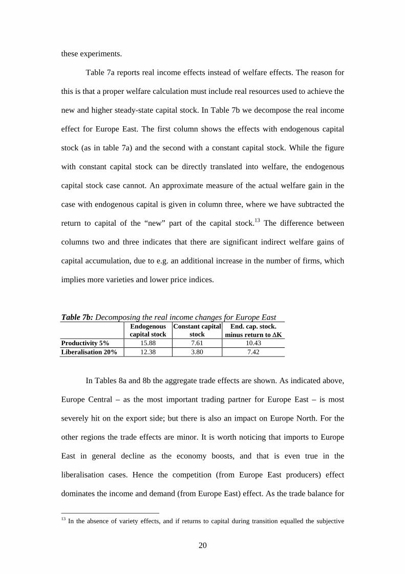
Table 7a reports real income effects instead of welfare effects. The reason for

this is that a proper welfare calculation must include real resources used to achieve the

new and higher steady-state capital stock. In Table 7b we decompose the real income

effect for Europe East. The first column shows the effects with endogenous capital

stock (as in table 7a) and the second with a constant capital stock. While the figure

with constant capital stock can be directly translated into welfare, the endogenous

capital stock case cannot. An approximate measure of the actual welfare gain in the

case with endogenous capital is given in column three, where we have subtracted the

return to capital of the “new” part of the capital stock.13 The difference between

columns two and three indicates that there are significant indirect welfare gains of

capital accumulation, due to e.g. an additional increase in the number of firms, which

implies more varieties and lower price indices.

Table 7b: Decomposing the real income changes for Europe East Endogenous

capital stock Constant capital

stock End. cap. stock.

minus return to ΔKProductivity 5% 15.88 7.61 10.43 Liberalisation 20% 12.38 3.80 7.42

In Tables 8a and 8b the aggregate trade effects are shown. As indicated above,

Europe Central – as the most important trading partner for Europe East – is most

severely hit on the export side; but there is also an impact on Europe North. For the

other regions the trade effects are minor. It is worth noticing that imports to Europe

East in general decline as the economy boosts, and that is even true in the

liberalisation cases. Hence the competition (from Europe East producers) effect

dominates the income and demand (from Europe East) effect. As the trade balance for

13 In the absence of variety effects, and if returns to capital during transition equalled the subjective

21

each region is kept unaltered in all scenarios, the counterpart of this pattern of changes

in manufacture trade must be a decline in net exports from the agriculture and/or

energy sector in Europe East.

Table 8a: Changes in total manufacturing exports (percent change from base case) Productivity Risk premium Liberalisation 2.5 % 5% -5 % -10% 10% 20%

EuropeW 0.14 0.29 0.10 0.20 0.20 1.41 EuropeC -1.64 -3.27 -1.03 -2.06 -2.35 -9.73 EuropeS -0.19 -0.39 -0.12 -0.23 -0.13 -0.42 EuropeN -0.82 -1.63 -0.50 -1.00 -0.43 -1.15 EuropeE 16.76 34.94 9.98 20.52 21.60 101.48 FormSov -0.25 -0.50 -0.15 -0.30 -0.28 -0.67 CSAsia -0.22 -0.44 -0.12 -0.25 -0.48 -1.06 SEAsia 0.03 0.07 0.02 0.05 -0.01 0.06 USACAN 0.03 0.06 0.03 0.06 -0.01 0.09 RestofW -0.20 -0.40 -0.12 -0.25 -0.16 -0.45 Table 8b: Changes in total manufacturing imports (percent change from base case)

Productivity Risk premium Liberalisation 2.5 % 5% -5% -10% 10% 20%

EuropeW -0.49 -0.95 -0.31 -0.62 -0.74 -2.64 EuropeC 0.87 1.82 0.53 1.08 1.39 7.14 EuropeS -0.11 -0.17 -0.08 -0.14 -0.23 -0.30 EuropeN -0.01 0.03 -0.01 -0.01 -0.34 -0.91 EuropeE -0.93 -1.85 -0.58 -1.16 -0.61 -4.98 FormSov 0.78 1.68 0.46 0.95 0.17 1.86 CSAsia 0.11 0.25 0.07 0.15 0.04 0.34 SEAsia -0.18 -0.34 -0.10 -0.21 -0.26 -0.74 USACAN -0.14 -0.27 -0.09 -0.17 -0.18 -0.45 RestofW 0.14 0.31 0.09 0.18 0.03 0.49

Sectoral Effects

Table 9 shows the sectoral production effects in Europe East. When studying the

sector-specific production effects, we should distinguish between three groups of

industries:

(i) Public and private services are non-traded. Hence, these industries

develop in accordance with domestic demand. The input-output structure of the

model, and the fact that private services are important inputs in other industries,

discount rate, this calculation would be exact.

22

explain part of the growth in production of private services. The increased demand for

services from an expanding manufacturing sector triggers the expansion of the service

sector, which reduces the price on services (due to IRS in production), and in turn

enhances the profitability of manufacturers.

(ii) Energy and agriculture are treated as perfectly competitive sectors in the

model; hence, these are fairly flexible, and will to a large extent serve as residuals.

Should other sectors become profitable enough to expand beyond the possibilities

provided by increased productivity and new investments, primary factors will have to

be drawn from the perfectly competitive sectors.

(iii) There are ten traded, manufactured goods. Given that the initial “shocks”

in terms of productivity improvements and additional resources are neutral across

sectors, it is interesting to see the significant differences in production effects:

Textiles and Transport equipment experience the highest growth effects, while

Leather and Machines experience strong growth in some of the cases. The results

indicate that successful transformation may have strong pro-competitive effects on

these sectors. However, industries are sensitive to different experiments. In relative

terms, Textiles and Leather respond most strongly to the liberalisation experiment.

This indicates the importance of market access for these sectors. Also from Table 5,

the high own-input share in Textiles may be noted, which implies potentially strong

agglomeration forces in this sector. An accompanying significant fall in Textiles

production in Europe Central (see Forslid et al, 1999a) also indicates that there is an

agglomeration in this sector in Eastern Europe. Transport Equipment shows more

comparable growth rates across all experiments. Here delocation from other regions is

more modest. What these sectors have in common is an extensive use of labour

relative to capital (see Table 6). However, the former is typically unskilled intensive

23

sectors, while the latter is typically skill-intensive. It might seem surprising that skill-

intensive sectors such as Transport equipment and Machines expand in Europe East,

which is a relatively less skill-abundant region. However, even though Transport

equipment and Machinery are relatively skill intensive compared to other sectors in

Europe East, they are significantly less skill intensive than the same sectors in the EU

(see Forslid et al, 1999a).

Table 9: Production effects in EuropeEast (percent change from base case) Productivity Risk premium Liberalisation 2.5 % 5% - 5 % - 10% 10% 20%

Public service 4.55 9.38 2.39 4.86 0.56 3.05 Private service 6.00 12.35 4.00 8.22 1.68 7.37 Textiles 14.00 28.84 8.75 17.93 42.08 179.16 Leather 10.61 21.99 6.73 13.86 12.09 44.03 Wood Prod. 7.94 16.32 5.03 10.30 2.81 12.89 Metals 12.30 24.93 7.96 16.14 4.66 15.94 Minerals 9.01 18.40 5.94 12.12 2.96 11.05 Chemicals 9.09 18.73 5.80 11.94 6.19 23.96 Food Prod. 7.29 15.32 4.51 9.38 3.63 16.91 Trans.Eq. 37.15 74.97 23.11 46.66 23.92 71.81 Machines 18.16 37.05 11.56 23.51 1.56 10.50 OtherMan 9.62 19.76 6.11 12.50 2.95 15.83 Agriculture -5.58 -11.33 -4.95 -9.93 -10.45 -46.92 Energy -4.28 -9.04 0.07 0.03 -14.82 -63.12

Factor prices

Table 10 shows the effect on factor prices in Europe East. Both unskilled and skilled

wages rise in the different transformation and integration cases, but skilled labour

experiences a significantly higher wage increase than does unskilled labour.

Table 10: Real wages in Europe East (percent change from base case)

Productivity Risk premium Liberalisation 2.5 % 5% - 5 % - 10% 10% 20%

Skilled labour

10.70 22.40 7.20 15.00 5.00 22.80

Unskilled labour

8.50 17.80 5.70 11.80 3.10 14.50

24

The impact on real wages in the transformation experiments related to productivity

and risk premium, is best explained by reviewing Table 6 on factor intensities and the

production effects in Table 9. In general we see that both unskilled- and skill-

intensive sectors expand, but the expansion of skill-intensive sectors is significantly

larger than that of unskilled-intensive sectors. In the liberalisation cases, the most

significant structural change is the reallocation of resources from the perfectly

competitive sectors (agriculture and energy) to the manufacturing and services

sectors. As the declining sectors – and in particular agriculture – are the least skill-

intensive sectors, this reallocation explains the relative factor price changes.

Sensitivity testing

Our experiments so far contain an element of sensitivity testing with respect to the

magnitudes of changes in productivity, risk premium and trade costs. It is well known,

however, that numerical results in the Dixit-Stiglitz framework may be highly

sensitive to the magnitude of the scale elasticities (σ). We have earlier pointed out that

in equilibrium there is a one-to-one relationship between the scale elasticity (a

technology parameter) and the elasticity of substitution (a demand related parameter)

in such models in equilibrium. While our simulations so far have been conducted with

scale elasticities based on the ranking by Pratten (1988), in this section we will

employ alternative values for σ taken from Martins, Scarpetta and Pilat (1996), who

estimate sectorial mark-ups (σ/(σ−1)) within 14 OECD-countries over the period

1970-92.14 For comparison, Table 11 displays the mark-ups used in the simulations

above as well as the values based on Martins, Scarpetta and Pilat. While the overall

14The matrix of mark-ups by Martins, Scarpetta and Pilat (1996) contains some empty cells due to missing observations. Francois (2000) runs cross-country regressions with sector and country dummies, and use the resulting coefficients to fill the empty cells. We use this matrix to calculate unweighted

25

levels are very similar, there are some significant sectoral differences. One example is

Transport equipment, which is a sector characterised by large (technological) scale

economies, but where fierce market competition forces mark-ups down.

Table 11: Mark-up Ratios

Pratten Martins,

Scarpetta and Pilat

Textiles 1.05 1.13 Leather and Products 1.05 1.15 Wood Products 1.14 1.19 Metals 1.19 1.19 Minerals 1.11 1.27 Chemicals 1.31 1.24 Food Products 1.09 1.14 Transport Equipment 1.35 1.12 Machinery 1.25 1.31 Other Manufacturing 1.09 1.18

In Tables 12 and 13 we display simulation results for real income and sectoral

production effects in Eastern Europe based on repeated experiments employing

elasticity estimates based on Martins, Scarpetta and Pilat instead of Pratten. As for

real income effects, a comparison of the results in Table 12 with those in Table 7a

indicates that our results are very robust – both in a qualitative and a quantitative

sense.

averages over the 14 countries for each sector.

26

Table 12: Real income effects II (percent change from base case) Productivity Risk premium Liberalisation 2.5 % 5 % -5.0 % -10 % 10 % 20 % EuropeW 0.02 0.04 0.01 0.02 0.01 0.04 EuropeC -0.07 -0.13 -0.04 -0.08 -0.07 -0.24 EuropeS -0.01 -0.01 -0.01 -0.01 0.00 -0.02 EuropeN -0.02 -0.05 -0.02 -0.03 -0.03 -0.14 EuropeE 8.07 16.89 5.10 10.55 2.60 10.77 FormSov -0.01 -0.01 -0.01 -0.01 0.00 -0.02 CSAsia -0.07 -0.14 -0.04 -0.09 -0.09 -0.30 SEAsia 0.01 0.01 0.00 0.00 0.01 0.01 USACAN 0.00 0.00 0.00 0.00 0.00 0.00 RestofW -0.02 -0.04 -0.02 -0.04 -0.01 -0.08

Turning to production effects by sector in Eastern Europe (see Table 13), we would a

priori expect the results to differ more from our previous results, because of the

differences in size and rankings of sectoral mark-ups. However, again the results in

the two transformation experiments on productivity and risk premiums appear to be

remarkably robust. In the trade liberalisation experiments there are more significant

changes – in particular for Textiles, Leather and Transport equipment. The

differences in the assumed mark-ups and hence elasticities are to a large extent

reflected in the simulation results. Martins et al report higher mark-ups for Textiles

and Leather, while their mark-up for Transport equipment is lower than the one

applied above. A lower mark-up – as in the Transport equipment case – implies a

higher elasticity of substitution and a more competitive market. Liberalisation would

typically yield stronger production effects in markets with a higher degree of

competition, and vice versa, and that is exactly what our simulations confirm. Textiles

and Leather, with less competitive markets according to the alternative assumptions,

show smaller production effects of liberalisation in Eastern Europe, while Transport

equipment, which is a much more competitive market under the alternative

assumptions, reveals significantly stronger production growth.

27

Table 13: Production effects in EuropeEast II (percent change from base case) Productivity Risk premium Liberalisation 2.5 % 5% - 5 % - 10% 10% 20%

Public service 4.70 9.68 2.48 5.04 0.49 2.27 Private service 6.23 12.84 4.15 8.52 1.71 6.48 Textiles 14.47 29.76 9.05 18.51 20.12 60.55 Leather 11.10 23.02 7.05 14.48 6.96 22.14 Wood Prod. 8.05 16.57 5.10 10.45 2.67 10.36 Metals 13.15 26.73 8.49 17.24 8.84 32.34 Minerals 8.84 18.02 5.82 11.86 4.20 15.51 Chemicals 9.67 19.94 6.16 12.69 5.23 16.44 Food Prod. 7.60 16.02 4.70 9.79 3.19 13.20 Trans.Eq. 42.08 85.74 26.12 53.02 60.77 229.87 Machines 18.99 38.74 12.08 24.55 5.63 24.79 OtherMan 9.84 20.24 6.25 12.77 3.35 13.15 Agriculture -6.17 -12.60 -5.30 -10.67 -10.40 -40.37 Energy -4.76 -10.20 -0.21 -0.62 -14.41 -54.17

5. Discussion and conclusions

In this paper we have presented model simulations for a set of scenarios involving the

transformation and integration of Europe East. Although the scenarios have been

specified in a stylised way, they might capture potentially important structural

changes. They might further indicate the relative importance of different reforms and

developments, and the very different effects Eastern transition may have across

sectors and regions.

Our simulations show that the neighbouring countries in Europe Central are

more affected than other European regions, and one feature that was not obvious ex

ante, is that the overall effect for Europe Central is negative. But even for Europe

Central, where some sectors may see successful transformation in Eastern Europe as a

threat, the overall effects in terms of real GDP are very small.

Simulations not reported in the paper show that adding Former Soviet Union

transition to Eastern European transition, has a negligible effect on all other regions

than the Former Soviet Union itself, which experiences a strong real income effect.

28

The reason for this being the region’s insignificant trade in manufacturing goods in

the benchmark case

Although our simulations do not cover agricultural policies, the implications

for agricultural markets in Europe may be of interest. The strong growth impetus to

manufacturing sectors in Europe East in our scenarios, actually implies increased

demand for imports of agricultural products to the region. In a more complete

scenario the overall effects on Europe East agriculture will depend on the direct

effects of reforming agricultural policies, and on the implied effects of transformation

of other sectors. Our analysis only includes the latter effect. However, the results

indicate that the “conventional wisdom” of an expected strong growth of agricultural

exports from east to west following an Eastern EU enlargement, is not necessarily

true.

The simulation results show a strong correlation between real income gains

and growth in the production of manufactures; this calls for an explanation, as such a

result would not appear in traditional trade models. However, our model differs from

traditional neo-classical comparative advantage models in many ways; in particular,

there are pecuniary externalities in manufacturing production. Hence, there are self-

reinforcing growth effects in manufacturing industries, which may give rise to cost

advantages, increased value added, and the type of correlation we observe between

manufacturing production and real income in the simulation results. Put differently,

we get rent-shifting effects, similar to the profit-shifting effects we know from

strategic trade policy analysis. Regions that get more of the industries with pecuniary

externalities gain, while other regions may lose.

To summarise, we can conclude that successful reforms and transformation in

Eastern Europe and Former Soviet Union are of huge importance for the economic

29

development in these regions, and may imply significant changes in the pattern of

specialisation and trade in these regions. However, in economic terms both regions

are too small to matter very much for the overall production and real income

elsewhere.

30

References Allen, C., M. Gasiorek and A. Smith (1998): “The competition effects of the single

market in Europe”, Economic Policy 27, pp 439 – 486. Baldwin, R.E. (1994): Towards an integrated Europe. CEPR. Baldwin, R. E. (1999): “Agglomeration and endogenous capital”, European Economic

Review 43, pp 253-280. Baldwin, R.E., R. Forslid and J.I. Haaland (1996): “Investment creation and

investment diversion in Europe”, The World Economy 19, pp 635-659. Baldwin, R.E., J.F. Francois and R. Portes (1997): “The costs and benefits of eastern

enlargement: the impact on the EU and central Europe.” Economic Policy, 24, 1997, pp 125 – 176.

Dixit, A. and J. Stiglitz (1997): “Monopolistic competition and the optimum product diversity”, American Economic Review 67, pp. 297 – 308.

Feenstra, R. C. (1997): “World Trade flows, 1970-1992, with Production and Tariff Data”, NBER Working Paper No. 5910.

Forslid, R., J.I. Haaland, K.H.M. Knarvik and O. Mæstad (1999a): “Modelling the economic geography of Europe: scenarios for location of production and trade in Europe”, SNF Report no. 67/99.

Forslid, R., J.I. Haaland and K.H.M. Knarvik (1999b): “A U-shaped Europe? A simulation study of industrial location”, CEPR Discussion paper no. 2247.

Francois, J.F. (2000): ”The Economic Impact of New Multilateral Trade Negotiations: Final Report”, Mimeo, Tinbergen Institute.

Fujita, M., P. Krugman and A.J. Venables (1999): The Spatial Economy: Cities, Regions and International Trade, MIT Press, 1999.

Gasiorek, M., A. Smith, and A.J. Venables (1991): "Competing the internal market in the EC: factor demands and comparative advantage," in Venables and Winters (eds) European integration: trade and industry, Cambridge University Press.

Gasiorek, M., A. Smith and A.J. Venables (1992): "'1992': trade and welfare - a general equilibrium analysis", in A.Winters (ed) Trade flows and trade policy after '1992', CEPR and Cambridge University Press.

Gasiorek, M. and A.J. Venables (1998): The welfare implications of transport improvements in the presence of market failure, unpublished manuscript.

Haaland, J. and V.D. Norman (1992): "Global Production Effects of European Integration”, in A. Winters (ed) Trade flows and trade policy after '1992', CEPR and Cambridge University Press.

Haaland, J. and V.D. Norman (1995): “Regional effects of European integration”, In Baldwin, Haarparanta and Kiander (eds.) Expanding membership of the European Union, Cambridge University Press.

Keuschnigg, C. and W. Kohler (1996): “Austria in the European union: dynamic gains from integration and distributional implications”, Economic Policy 22, 1996, pp. 155– 212.

Keuschnigg, C. and W. Kohler (1998): “Eastern enlargement of the EU: how much is it worthfor Austria”, CEPR Discussion paper no 1786, 1998.

Krugman, P. R. (1991): “Increasing Returns and Economic Geography”, Journal of Political Economy 99, 483-499.

Martins J.O. Scarpetta S. and D. Pilat,(1996): ”Mark-up Ratios in Manufacturing Industries, Estimates for 14 OECD Countries”, OECD Working paper no.162.

de Ménil, G. (1999): ”Real capital market integration in the EU: How far has it gone? What will the effect of the Euro be?, Economic Policy 28, 1999, pp. 167-204.

31

Pratten, C. (1988): “A survey of economies of scale”, in Commission of the European Communities: Research on the cost of non-Europe, Vol. 2: Studies on the economics of integration, Luxembourg 1988.

Lewis, W.A. (1954): “Economic Development with Unlimited Supplies of Labor”, The Manchester School, 22, 1954, pp. 139-191.

Venables, A. (1996): “Equilibrium location of vertically linked industries”, International Economic Review, 37, 1996, pp. 341 – 359.

Young, A. (1995): “The tyranny of numbers: Confronting the statistical realities of the EastAsian growth experience. ”Quarterly Journal of Economics, 110, 1995, pp.641-80.