1

INTEGRATING SIMULATION AND DESIGN OF EXPERIMENTS TO IDENTIFY FACTORS FOR LAYOUT DESIGN

Kaushik Balakrishnan, Sam Anand Computer-Aided Manufacturing Lab

Industrial Engineering Program University of Cincinnati, Cincinnati, OH 45221-0116

David Kelton Department of Quantitative Analysis and Operations Management

College of Business Administration University of Cincinnati, Cincinnati, OH 45221-0130

2

Abstract

In this paper, the facilities design of a manufacturing layout is conducted by integrating

simulation and design of experiments to study the influence of process parameters on the

performance of the plant. This research study involves a shop floor wherein the parts

contributing to 75% – 80% of the annual revenue are analyzed. This is achieved by

selecting a few potential parameters/factors that could affect the time in system of these

parts in the plant, and a 28 factorial experimental design is conducted to measure the main

effects and interactions between these factors. The eight experimental factors include the

location of machines, batch sizes of the parts, downtimes and setup times on machines,

number and type of transporters, work-in-process container size, and machine utilization.

The responses from the designed experiment help us relate the factors affecting the

output of each part to improve the productivity of the plant.

Keywords: Facilities Design, Simulation, and Design of Experiments

3

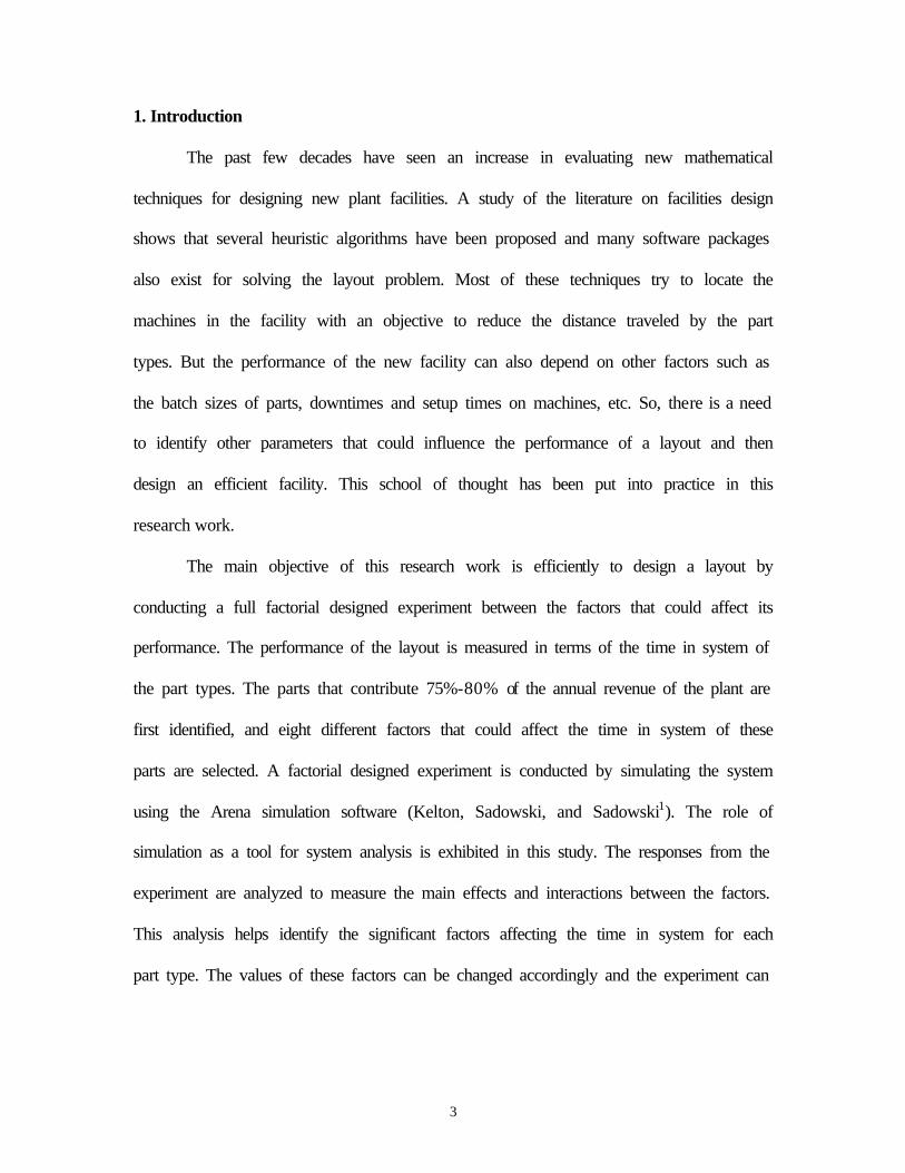
1. Introduction

The past few decades have seen an increase in evaluating new mathematical

techniques for designing new plant facilities. A study of the literature on facilities design

shows that several heuristic algorithms have been proposed and many software packages

also exist for solving the layout problem. Most of these techniques try to locate the

machines in the facility with an objective to reduce the distance traveled by the part

types. But the performance of the new facility can also depend on other factors such as

the batch sizes of parts, downtimes and setup times on machines, etc. So, there is a need

to identify other parameters that could influence the performance of a layout and then

design an efficient facility. This school of thought has been put into practice in this

research work.

The main objective of this research work is efficiently to design a layout by

conducting a full factorial designed experiment between the factors that could affect its

performance. The performance of the layout is measured in terms of the time in system of

the part types. The parts that contribute 75%-80% of the annual revenue of the plant are

first identified, and eight different factors that could affect the time in system of these

parts are selected. A factorial designed experiment is conducted by simulating the system

using the Arena simulation software (Kelton, Sadowski, and Sadowski1). The role of

simulation as a tool for system analysis is exhibited in this study. The responses from the

experiment are analyzed to measure the main effects and interactions between the factors.

This analysis helps identify the significant factors affecting the time in system for each

part type. The values of these factors can be changed accordingly and the experiment can

4

be iteratively conducted. Based on the results from these experiments, the new facility

can be designed efficiently.

This research work is carried out for an automotive accessories plant. The

anonymity of the plant facility, part, and machine names is maintained in this research

work. However, the information used for conducting this research work is real and not

hypothetical.

Section 2 contains a literature survey of existing facilities-design techniques.

Section 3 describes the problem description and data collection, data analysis, and gives

an overview of the potential factors considered in this experiment that could affect the

given system. Section 4 discusses the type of experimental design conducted, and also

gives a brief procedure of how the system was modeled. This is followed by Section 5,

which describes the analysis of the responses obtained for each part type from the

designed experiment. Finally, the conclusions and the application areas for this research

are described.

2. Facilities Design and Literature Review

The determination of the best layout for a facility is a classical industrial-

engineering problem. The prime interest in a facilities-design problem is to determine a

layout that optimizes some measure of production efficiency. The layout problem is

applicable to many environments like warehouses, banks, airports, manufacturing

systems, etc. Each of the above applications has distinct characteristics. Some of the

common objectives in any facilities-design problem as seen in Nahmias2, would be to

minimize cost investment for production, to utilize available space efficiently, to

5

minimize material handling cost, and to reduce work in process. As noted before, this

research work involves a facilities-design problem for a manufacturing facility where the

main objective is to minimize the time in system of the parts.

Extensive research has been done in designing layouts, including recent studies to

compare the performance of process layouts and cellular layouts. Earlier concepts that

cellular layouts outperform job-shop layouts in all aspects have been demonstrated to be

false. Flynn and Jacobs3 have done a comparison between job-shop layout and group-

technology layout using simulation. Their study reveals that the performance of group

technology was better in terms of average set-up time and average distance traveled per

move, but there were serious problems in the performance of group-technology shops in

other respects. This was attributed to long part queues in shops having dedicated

machines. This in turn increased the average time in system for parts being produced in

the cellular layout. Burgess, Morgan and Vollmann4 have also done a study that

compares a factory structured as a traditional job shop and as a hybrid factory containing

a cellular manufacturing unit. A systematic evaluation of cellular manufacturing was

conducted and the results revealed the particular circumstances that favored the use of

group technology. Shambu and Suresh5 have done a comparative study of hybrid

cellular manufacturing systems with traditional job-shop layouts under a variety of

operating conditions. Their study was conducted for the entire shop floor and revealed

that the performance of the remainder of the shop deteriorated with increasing conversion

of functional layouts into cellular manufacturing due to erosion of pooling synergy.

Studies have also identified methods to increase the performance of cellular

layouts. Sassani6 conducted a simulation experiment to demonstrate that the utilization of

6

group-technology cells can be improved through sub-batch workload transfer. The study

also showed that a detailed and practically oriented computer-simulation analysis could

be a useful aid in management decision-making. Several scheduling heuristics have also

been proposed for cellular manufacturing environments. Mahmood, Dooley and Starr7

proposed dynamic scheduling heuristics for manufacturing cells and showed that these

rules increase the performance of the cell layouts.

Unlike previous studies, the research reported here is undertaken to demonstrate

that different manufacturing parameters including the location of machines, batch sizes of

parts, downtimes of machines, etc. can influence the design and performance of layouts

for manufacturing facilities.

3. Problem Description

Our objective is to design an efficient layout with appropriate values for the

process parameters, so that the flow time of the parts is minimized. Flow time is the time

that a part spends in a system, from the raw-materials stage to the finished-goods area.

The process parameters include the location of machines, batch sizes, work in process,

machine downtimes, transporters, etc. The problem is solved by identifying different

parameters that could influence the flow time of the parts and then simulating the model

using different levels of these parameters. The responses from the simulation are then

studied using design of experiments to analyze the main and interaction effects of these

parameters. It should be noted that the approach and the methods used in this research

problem could also be applied to a wide class of manufacturing systems. This section

describes the preliminary analysis done before simulating the model. It includes the

7

problem definition, data collection, data analysis, part routings, and a brief description of

the potential parameters that could influence the flow time of the parts.

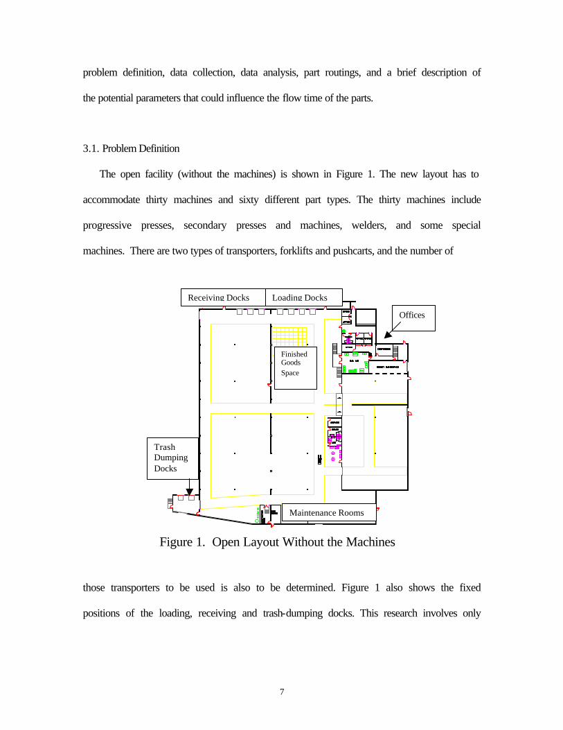
3.1. Problem Definition

The open facility (without the machines) is shown in Figure 1. The new layout has to

accommodate thirty machines and sixty different part types. The thirty machines include

progressive presses, secondary presses and machines, welders, and some special

machines. There are two types of transporters, forklifts and pushcarts, and the number of

those transporters to be used is also to be determined. Figure 1 also shows the fixed

positions of the loading, receiving and trash-dumping docks. This research involves only

Receiving Docks Loading Docks

Trash Dumping Docks

Offices

Finished Goods Space

Maintenance Rooms

Figure 1. Open Layout Without the Machines

8

the location of machines and it is assumed that the locations of the offices, restrooms,

tool maintenance rooms, and other auxiliary equipment have been decided.

3.2. Data Collection and Analysis

Data collection is one of the first steps involved in solving a manufacturing layout

problem. The accuracy and the extent of the data collected reflect the precision of the

results. It is important that all the necessary data required for modeling the layout be

collected for the parts that will be manufactured and the machines that will be used for

production during the time horizon for which the layout is planned. So, proper analysis of

the collected data is required before modeling the layout.

3.2.1. Data Collection

The basic data were collected from personnel on the shop floor: operators,

supervisors, and process managers, and was directed to the management information

systems department. The dimension of the open facility was first collected. The data on

the sixty parts were their routings, sales volume, sales price, and part life. (Part life is the

number of years it will be produced before it becomes extinct.) The data collected on the

machines were their dimensions, process times for the parts they processed, downtimes,

setup times, and maintenance times. The speed and downtimes of both types of

transporters is collected. The speed and capacity of the washers and the space available

for finished goods inventory is also gathered.

9

3.2.2. Data Analysis

The first step in data analysis is to identify the top parts in terms of their contribution

to the annual revenue of the company. This is done by Pareto analysis, which states that a

company that makes multiple products often generates most of its revenues, say 80%,

from 20% of its products. Figure 2 shows a pie chart indicating the distribution of parts

according to their annual revenue contribution.

The first ten parts, namely part 1 to part 10, contribute more than 75 % of the

revenue, so these parts are chosen for further investigation. It was ensured that these parts

would be produced for at least five years in the new layout.

Figure 2. Contribution of Parts Towards Annual Revenue

26%

Part 2

Part 1

16 %

Part 3

8 % Part 4 5 %

Part 7 3 %

Part 9 2 %

Part 10

2 %

Part 5

5 %

Part 8 4 %

5 % Part 6

10

3.3. Part Information

Table 1 shows the part information for the top ten parts chosen above. This table

indicates the part routing, capacity of the machines per cycle, the process times and the

setup times of the machines in minutes. Presses 1 to 9 are considered progressive

machines, while all other machines are secondary machines.

Part number Part routing Capacity/ Process timecycle in minutes Frequency Duration

(in minutes) (in minutes)Part 1 Press 1 1 0.167 500 20

Press 9 1 0.167Press 10 1 0.167Washer 1Press 11 1 0.167Press 12 1 0.167

Part 2 Press 2 2 0.0125 480 20Washer 2

Part 3 Press 3 1 0.0125 400 30Press 13 1 0.05

Special M/c 1 1 0.05Washer 3

Part 4 Press 5 1 0.026 480 20Special M/c 2 1 0.2

Part 5 Press 8 1 0.0357 300 20Part 6 Press 4 1 0.023 500 20

Washer 4Part 7 Press 6 1 0.0333 480 20

Welder 1 1 0.3Part 8 Press 7 1 0.0275 500 20

Hyd. Press 1 1 0.15Hyd. Press 2 1 0.15Hyd. Press 3 1 0.15Hyd. Press 4 1 0.15Hyd. Press 5 1 0.15

Part 9 Press 2 2 0.0125 450 20Washer 2

Part 10 Press 6 1 0.0333 480 20Welder 1 1 0.3

Setup time in minutesPart information

Table 1. Part Information.

11

3.4. Parameters

This section describes the potential parameters that could affect the flow time of

parts. Eight different parameters, namely layout (location of machines), batch sizes, WIP

container size, number of transporters, types of transporters, machine downtimes, coil-

change times, and machine utilization, are chosen and the experiment is conducted with

two levels for each factor. Table 2 shows the coding for the values corresponding to the

“+” and “-” levels for each of the eight parameters.

3.4.1. Layout

This parameter refers to the location of machines in the facility. This is one of the

important parameters that could affect the flow time of the parts. This is primarily

Table 2. Values of the Parameters.

Codes Values1 Layout - Job-shop layout

+ Hybrid layout2 Batch sizes1 - High value

+ Low value3 WIP container - High value

size1 + Low value4 Type of - Push-cart

transporter + Forklift5 Number of - 4

transporters + 26 Machine - High value

downtimes1 + Low value7 Coil Change - 30 minutes

time2 + 5 minutes8 Machine - 90%

Utilization + 60%

Factors

1 - Refer to their individual tables2- Applicable only for the progressive presses

12

because the objective is to design an efficient layout to reduce the time spent by the parts

in the system. As seen in table 2, two levels of this factor are taken into consideration,

process layout and hybrid layout. Though the hybrid layout could outperform the process

layout, the given system is not simple enough to decide if this factor alone would affect

the flow time for all the ten parts. It should be remembered this was the objective of the

research problem.

Process layout, also known as job-shop layout, is one in which similar machines

are located together. This would imply that the progressive presses are located in one

portion of the facility and the secondary machines/presses are located at the other end of

the facility. Figure 3 shows a job-shop layout.

Finished Goods Space

Maintenance Rooms

Trash Dumping Docks

Receiving Docks Loading Docks

Offices

Primary machines

Secondary Machines

Figure 3. Job-Shop Layout with Progressive and Secondary Machines at Different Sides.

13

The hybrid layout combines the process and cellular layouts. Cellular layout is based on

group-technology principles, where the machine cells and part families that are

independent of the others are identified and a number of subsystems are formed. Figure 4

shows a hybrid layout where a few machines are grouped together as cells, and the others

are placed as in a job-shop layout.

Individual Cells

Secondary Machines

Maintenance Rooms

Trash Dumping Docks

Receiving Docks Loading Docks

Offices

Figure 4. Hybrid Layout Showing a Combination of Job-Shop and Cellular Layouts.

14

This hybrid layout is designed by forming a part-machine matrix, which indicates the

volume and flow of parts between machines. From this matrix, the part families

processed in unique machine cells are easily identified and thus cells are formed. But not

all the parts are produced in unique machine cells, which lead to the combination of a

job-shop and a cellular layout known as the hybrid layout. The other techniques used to

design the hybrid layout are not described in detail in this paper.

3.4.2. The Other Seven Parameters

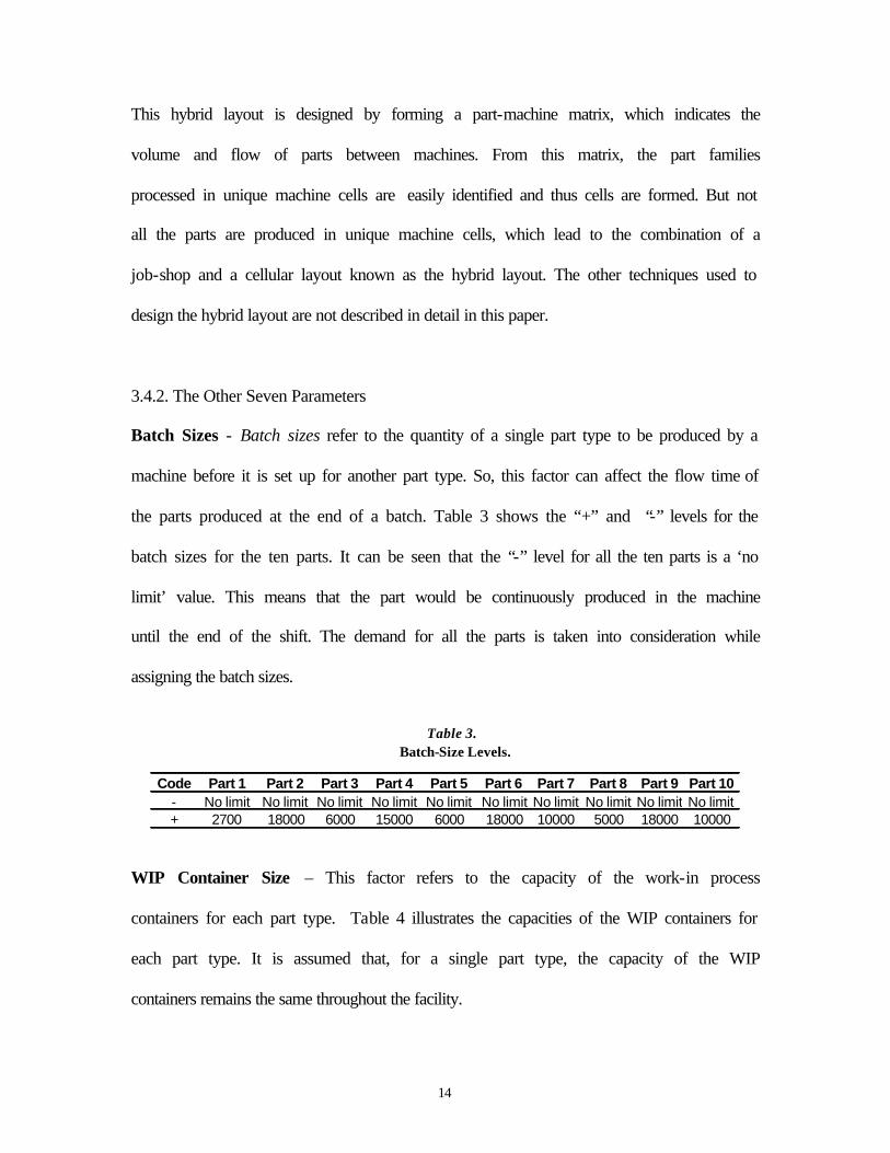
Batch Sizes - Batch sizes refer to the quantity of a single part type to be produced by a

machine before it is set up for another part type. So, this factor can affect the flow time of

the parts produced at the end of a batch. Table 3 shows the “+” and “-” levels for the

batch sizes for the ten parts. It can be seen that the “-” level for all the ten parts is a ‘no

limit’ value. This means that the part would be continuously produced in the machine

until the end of the shift. The demand for all the parts is taken into consideration while

assigning the batch sizes.

WIP Container Size – This factor refers to the capacity of the work-in process

containers for each part type. Table 4 illustrates the capacities of the WIP containers for

each part type. It is assumed that, for a single part type, the capacity of the WIP

containers remains the same throughout the facility.

Table 3. Batch-Size Levels.

Code Part 1 Part 2 Part 3 Part 4 Part 5 Part 6 Part 7 Part 8 Part 9 Part 10- No limit No limit No limit No limit No limit No limit No limit No limit No limit No limit+ 2700 18000 6000 15000 6000 18000 10000 5000 18000 10000

15

Type and Number of Transporters – This is an important factor because the raw

materials, work in process and the finished goods are moved via transporters, so

availability of transporters can influence the average flow time of the parts. The two

types of transporters, forklifts and pushcarts, differ by their speed. The speed of the

forklift is 444.44 feet/minute and speed of the pushcart is 266.66 feet/minute. The

number of transporters is varied between two and four.

Machine Downtimes – Table 5 indicates the downtimes of the progressive and the

secondary machines in terms of a percentage. It can be seen that the progressive

machines have more downtime than the secondary machines. It is assumed that the

interarrival times between machine failures and the repair times are deterministic,

consistent with our data from the plant. This factor would give an indication to the plant

manager to check if preventive maintenance measures should be carried out in order to

reduce machine downtimes.

Table 4. WIP-Container-Size Levels.

Code Part 1 Part 2 Part 3 Part 4 Part 5 Part 6 Part 7 Part 8 Part 9 Part 10- 300 3600 5000 5000 3000 5000 3400 500 3600 3400+ 1 1800 2500 2500 1500 2500 1700 100 1800 1700

Table 5. Downtime Levels.

Code Progressive M/c's Secondary M/c's- 33.33% 10%+ 8.33% 5%

16

Coil-Change Time – This factor is applicable only for the progressive presses. The raw

material for these progressive presses is in the form of large sheet-metal coils and so a

setup time is involved to replace the coils. The time taken for changing the coil could be

reduced from 30 minutes to 5 minutes by procuring an automatic coil changer that can

hold two coils at a time. After the machine runs out of the first coil, the second coil can

be placed immediately, which in turn reduces the coil-change time.

Machine Utilization – As seen in Table 2, the utilization of all the machines is set at

levels of 90% and 60%. This factor should not be confused with the machine downtimes.

The machine utilizations are assigned with the consultation of the plant managers and

supervisors. The effect of this factor on the flow time of the parts would indicate if the

machines have been utilized properly and if not, how much less or more utilization is

required.

4. Experimental Design

The system under study is quite complex, which makes it difficult for a plant

manager to identify the parameters that could affect the flow time of the ten part types. In

the case of a job-shop layout, all the parts have to be moved from the progressive presses

to the secondary machines. This could depend heavily on the availability of transporters,

but it is difficult to say if this factor alone could influence the flow time of the parts. In

fact, the layout is also considered as a factor in this problem. In the case of a hybrid

layout, the transporter might not be a big factor because of the presence of machine cells,

where the parts move within these cells. This complexity in identifying a factor can be

solved by using design of experiments. The output obtained from the experimental design

17

would help the plant managers to identify the main factors responsible for affecting the

flow time and also indicate the interactions between these factors. This, in turn, would

help him to change the values for these factors to reduce the flow time of parts.

The part routing (Table 1), the batch sizes (Table 3) and the WIP container

information for part 2 and part 9 are the same. So, it is assumed that the output obtained

for part 2 would be same for part 9 and the same can be noted for part 7 and part 10 and

so further analysis is done only for first eight part types instead of the original ten. This

section describes the type of experimental design conducted and also the method by

which it is carried out.

4.1. 28 Factorial design experiment

The input parameters that compose the given system are known as factors of the

experimental design. All the factors considered in this experiment are controllable in the

sense that the operators and the plant managers can bring about a change in the values of

these parameters. As seen in the previous section, we have eight different factors, each

varying between two levels. This leads to a 28 factorial design experiment, where an

experiment is conducted with all 256 combinations of the eight factors. A design matrix,

as shown in Table 6, is formed to indicate each combination with the different

combinations of the eight factors. The “+” and “-” signs indicate the values assigned for

these factors and can be referred from Table 2. The output performance measure is the

flow time of the parts and it is known as the response of one experiment. So eight

responses, corresponding to the eight parts, are collected from each experiment, and are

tabulated.

18

4.2. Conducting the Experiments

The given system is modeled using the Arena 3.0 simulation software1. As noted

before, only the equipment processing the eight part types was modeled. This leads to

the modeling of eight progressive presses, fourteen secondary machines, and four

washers, which correspond to eight different manufacturing lines. The machine

downtimes, utilization and the coil-change time are modeled as individual downtimes on

the machines. The washers are modeled as accumulating conveyors and are defined by

their speed and cell size. The transporters are defined by their speed and capacity, and the

downtime on the transporters is also modeled. If the parts require a transporter, they are

batched according to their WIP container size and wait for a transporter according to the

queue discipline. The priority is cyclical for all the part types requesting a transporter.

Distance sets are suitably defined to indicate the distances between the machines, loading

docks, receiving docks, and the finished-goods area. It is assumed that there is no

shortage of raw materials. The finished-goods area is large enough to accommodate the

varying batch sizes of all the part types.

Table 6.

Design Matrix and Responses for Part 1. Response

Layout Batch sizes WIP container Type of Number of Downtimes Coil change M/c (in minutes)size transporter transporter on M/c time utilization Part 1

Scenarios1 -1 -1 -1 -1 -1 -1 -1 -1 1022 1 -1 -1 -1 -1 -1 -1 -1 101.983 -1 1 -1 -1 -1 -1 -1 -1 57.0254 1 1 -1 -1 -1 -1 -1 -1 56.9915 -1 -1 1 -1 -1 -1 -1 -1 101.99. . . . . . . . . .. . . . . . . . . .

255 -1 1 1 1 1 1 1 1 53.324256 1 1 1 1 1 1 1 1 53.5

Factors

19

The model was run using a Pentium 300 MHZ processor with 128 MB of RAM.

Each experiment was run for one simulated day (1440 minutes) and it took approximately

15 minutes of computer time for each of them. The run length of 1440 minutes for each

experiment was chosen from proper understanding of the day-to-day operations occurring

in the plant. Moreover, the batch sizes of the parts were selected for one day according to

the demand. Since all the input values to the simulation are deterministic, each

experiment is run only once and is not replicated. The flow times, known as responses in

the experimental design, for all the eight parts were noted after each experiment and

tabulated for further analysis.

5. Interpreting the Responses

It is important to analyze properly the results obtained from the above

experiments to establish the influence of the factors for the eight part types. The effects of

the factors can be categorized into their main effects and the interactions among them.

This section explains the main effects of the factors on the flow time of all the eight parts

and also the interactions among the factors influencing the output.

The main effect of a factor is the average change in the output due to the factor

shifting from its “-” level to its “+” level, while holding all other factors constant. Table 7

Table 7. Top Three Factors Affecting the Flow Time of the Top Eight Parts, Arranged in

Decreasing Order of Effectiveness.

1 2 3Part 1 Batch sizes M/c utilization WIP container sizePart 2 Batch sizes WIP container size Downtimes on m/cPart 3 Layout WIP container size Downtimes on m/cPart 4 WIP container size Layout Type of transporterPart 5 Batch sizes Downtimes on m/c Coil change timePart 6 WIP container size Layout Type of transporterPart 7 WIP container size Layout Number of transportersPart 8 Batch sizes WIP container size Layout

Factors

20

indicates the top three factors influencing the flow time of the parts. It can be seen that

each part type generally has a different sequence of factors affecting its flow time.

Analysis of the main effects alone would not suffice as the effect of one factor

could depend on the level of some other factor, which is interaction between the factors.

In this study, interactions between the factors are computed starting from two-factor

interactions all the way up to the eight-factor interaction. This would help to conduct a

thorough analysis of identifying the most significant factor affecting the time-in-system

for each part type.

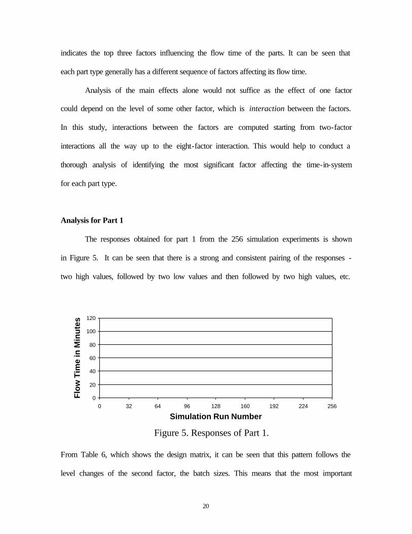
Analysis for Part 1

The responses obtained for part 1 from the 256 simulation experiments is shown

in Figure 5. It can be seen that there is a strong and consistent pairing of the responses -

two high values, followed by two low values and then followed by two high values, etc.

From Table 6, which shows the design matrix, it can be seen that this pattern follows the

level changes of the second factor, the batch sizes. This means that the most important

Figure 5. Responses of Part 1.

0

20

40

60

80

100

120

0 32 64 96 128 160 192 224 256

Simulation Run Number

Flow

Tim

e in

Min

utes

21

factor affecting the flow time of part 1 is batch sizes. Thus, the plant manager should

decrease the batch sizes of part 1 in order to reduce its flow time. It is a well known that

reducing the batch size of a part will reduce its flow time, but this experiment also

ensures that the demand of the part is satisfied.

Figure 6 shows the main effects and interactions between the factors for part 1. As

inferred before, the batch sizes play a significant role in determining the flow time for

part 1. This is because the value of the main effect of the second factor (batch sizes) is

-38, which completely overwhelms the other main effects and all interactions. The value

of this main effect being negative indicates that the low value (“+” coding) of the batch

sizes would decrease the flow time of part 1. Since the objective is to reduce the flow

time of the part, lower batch sizes should be used.

The next important observation on the main effects is the machine utilization, as

seen from Figure 6 having a value of -8.75. This can also be inferred from Figure 5,

where the responses have a different pattern after the first 128 experiment runs. The

Figure 6. Main Effects and Interactions of the Factors on Flow Time of Part 1

-50

-40

-30

-20

-10

0

10

20

Effect Label

Eff

ect o

n Fl

ow T

ime

Main effects

Two to eight factor interactions

1 2 3 4 5 6 7 8

22

negative value of the main effect of machine utilization indicates that the utilization of

the machines should be decreased from 90% to 60% to achieve a reduction in flow time.

It should be noted that the interaction between the batch and machine utilization has a

value of +8.74 that ties with the main effect of machine utilization. The positive sign of

the batch size and machine utilization interaction indicates that having these two factors

at the same level (so their product is +1) tends to increase flow times. So, having these

two factors at opposite levels, and other things being equal, would help to reduce the flow

time.

When factors have significant interactions, interpretation of the main effects

becomes unclear since the response is nonlinear in one or both of the factors. But in this

case since the magnitude of the main effect of batch size is much bigger than the other

values, it is clear that smaller batch sizes have a significant effect on reducing the flow

time. Though setting the machine utilization at its “+” level (60%) lowers the flow time

by about 8.75, the unfavorable interaction with the small batch size increases the flow

time by about the same amount (9). Also, the main effects of other factors and the two-

factor interaction effects of these factors are negligible. The three-factor to eight-factor

interactions do not have any significant contribution and are almost zero. So, a practical

conclusion could be that, if the plant manager doesn’t have the luxury of decreasing batch

sizes for some other reason, then low utilization would be helpful. The layout is not an

important factor for this part because there is little change in the two layouts for the

machines processing this part type.

23

Analysis for Part 2

Figure 7 shows the responses obtained for part 2 from the simulation runs. As

seen in the previous case, that there is a strong and consistent pairing of the responses -

two high values, followed by two low values and then followed by two high values, etc.

So, once again the batch sizes (the second factor) become the most important factor

affecting the flow time of part 2.

This can also be inferred from Figure 8, which shows the main effects and

interactions of the factors on the flow time of part 2. The value of the effect of batch sizes

is -147 and it is the most dominating effect for part 2. Since this value is negative, smaller

batch sizes (“+” coding) should be used to reduce the time in system. The next most

significant factor affecting the flow time for part 2 is the WIP container size. Figure 7

also shows that the responses follow a repeating pattern after every four values.

The value of its main effect is -17.77. Since this factor has a negative effect on the

flow time (as seen from Figure 8), the number of parts batched between the machines

0

50

100

150

200

250

300

350

400

450

0 32 64 96 128 160 192 224 256

Simulation Run Number

Flow

Tim

e in

Min

utes

Figure 7. Responses of Part 2.

24

should be reduced to reduce the flow time of part 2. Figure 8 also shows that the

interactions (two-factor to eight-factor) do not have a significant effect on the flow time.

So, the main objective of the plant managers would be to reduce the batch sizes. Also,

since the information for part 2 and part 9 are the same, the same conclusion applies to

part 9 also.

Analysis for Part 3

Figure 9 shows the main effects and interactions for part 3. At least five factors

have significant effects on the flow time of this part type. The most significant factor is

the layout of the machines producing the part type. The value of this effect is -262 and

since it is a negative value, this means that the layout should be changed from the job-

shop to the hybrid layout to decrease flow time.

Figure 8. Main Effects and Interactions of the Factors on Flow Time of Part 2

-160

-140

-120

-100

-80

-60

-40

-20

0

20

Effect Label

Eff

ect o

n Fl

ow T

ime

Main effects

Two to eight factor interactions

1 2 3 4 5 6 7 8

25

The next most significant factor is the WIP container size (having a main effect of

-116), which nearly ties with the main effect of the machine downtimes (value of -114).

The negative values of the main effects for these two factors suggest that the decrease in

the WIP container size and the machine downtimes would decrease the flow time for

part 3.

The next important observation is that the two-factor interaction between layout

and WIP container size has a value of +94. The positive value indicates that if these two

factors are both at their “+” or “-” levels together, this tends to increase the flow time of

this part, which is undesirable. Also, the main effects of coil change time and batch sizes

have values of -79 and -49 respectively. Thus, decrease in coil-change time and batch

sizes would reduce the flow time of this part. The other two-factor interactions and the

three to eight factor interactions do not have significant effects on the flow time. So,

since the main effect of layout overshadows all the other effects, the plant managers

should design a cellular layout rather than a job-shop layout to produce this part type.

Figure 9. Main Effects and Interactions of the Factors on Flow Time of Part 3

-300

-200

-100

0

100

200

Effect Label

Effe

ct o

n Fl

ow T

ime

Main effects

Two to eight factor interactions

1 2 3 4 5 6 7 8

26

For part 4, the WIP container size (-247) and the layout (-75) are the two most

significant factors affecting its flow time. The interaction between these two factors also

has some effect (+24) on the flow time. But the main effect of WIP container size

overshadows the other effects and the priority would be to reduce the WIP container size.

The flow time of part 5 is significantly affected by batch sizes (-90) and machine

downtimes (-69). Since there is some positive interaction between these two factors

(+30), the plant manager should use his discretion when trying to reduce the flow time for

this part.

Similar inferences can be made for the other part types. The plot diagrams

showing the main effects for each part type should be properly interpreted with reference

to the coding table (Table 1). The significant factors affecting the flow time of these parts

can be seen from Table 7. Due to the enormity of information, the response plots and the

main effects plots are not shown for the other part types, but can be seen in Kaushik8.

6. Concluding Remarks

The factors affecting the flow time of each of the top ten parts have been

identified. The next step would be to eliminate the least significant factors, manipulate

the values of other important factors, and conduct further experiments iteratively to

obtain better results. It is left to the discretion of the plant manager in selecting the

significant factors during the iterative process. If there is a conflict in the layout of

machines between two parts, the part contributing to higher annual revenue should be

given the top priority. At the end of this process, he would be able to design an efficient

layout and assign suitable values for the process parameters. The number and type of

27

transporters required can be inferred from the responses. This work demonstrates that the

manufacturing parameters also should be considered before designing the layout for a

facility.

This research has integrated simulation and design of experiments to identify the

parameters that would be responsible for affecting the flow time of parts in a plant layout.

The reduction of flow time essentially implies that the parts are being produced faster and

the work-in-process is also being reduced. This approach can be widely used for other

applications that have an objective of reducing/increasing an output depending on a few

parameters. Some potential applications could be for a bank or a department store, where

the objective is to reduce the time in system of the customers.

28

References

1. W. David Kelton, Randall P. Sadowski and Deborah A. Sadowski, “ Simulation with

Arena”, McGraw- Hill, 1998.

2. Steven Nahmias, “Production and Operations Analysis”, 3rd edition, McGraw-Hill,

1997, 561-573.

3. Barbara B. Flynn and F. Robert Jacobs, “A simulation comparison of group

technology with traditional job shop manufacturing”, International Journal of

Production Research, (v24, n5, 1986), 1171-1192.

4. A.G. Burgess, I. Morgan and T.E. Vollmann, “Cellular Manufacturing: its impact on

the total factory”, International Journal of Production Research, (v31, n9, 1993), 2059-

2077.

5. Girish Shambu and Nallan C. Suresh, “Performance of hybrid cellular manufacturing

systems: A computer simulation investigation”, European Journal of Operational

Research, (v120, n2, 2000), 436-458.

6. F. Sassani, “A simulation study on performance improvement of group technology

cells”, International Journal of Production Research, (v28, n2, 1990), 293-300.

7. Farzad Mahmoodi, Kevin J. Dooley and Patrick J. Starr, “An investigation of dynamic

group scheduling heuristics in a job shop manufacturing cell”, International Journal of

Production Research, (v28, n9, 1990), 1695-1711.

8. Kaushik Balakrishnan, “Integrating Simulation and Design of Experiments to Identify

Factors for Layout Design”, M.S. Thesis (Cincinnati, OH, University of Cincinnati,

2000).

29

9. Averill M. Law and W. David Kelton, “Simulation Modeling and Analysis”, 3rd

edition, McGraw-Hill, 2000.