Integrating Broad-Band High-Fidelity Acoustic Emission Sensors and Array Processing to Study Drying Shrinkage Cracking in Concrete

Gregory C. McLaskeya,1, Steven D. Glasera, Christian U. Grosseb

aDepartment of Civil and Environmental Engineering, University of California, Berkeley, USA bDepartment of Non-Destructive Testing and Monitoring; Material Testing Institute, University of Stuttgart,

Pfaffenwaldring 4, Stuttgart, Germany

Abstract Array processing of seismic data provides a powerful tool for source location and identification. For this method to work to its fullest potential, accurate transduction of the unadulterated source mechanism is required. In our tests, controlled areas of normal-strength concrete specimens were exposed to a low relative humidity at an early age to induce cracking due to drying shrinkage. The specimens were continuously monitored with an array of broad-band, high-fidelity acoustic emission sensors contrived in our laboratory in order to study the location and temporal evolution of drying shrinkage cracking. The advantage of the broadband sensors (calibration NIST-traceable) compared to more traditional acoustic emission sensors is that the full frequency content of the signals are preserved. The frequency content of the signals provides information about the dispersion and scattering inherent to the concrete, and the full unadulterated waveforms provide insight into the micromechanisms which create acoustic emissions in concrete. We report on experimental and analytical methods, event location and source mechanisms, and possible physical causes of these microseisms. Keywords: acoustic emission, microseismic, sensors, array processing, signal processing, concrete, wave propagation

1. Introduction The method of acoustic emissions (AE) has been used to noninvasively evaluate materials ranging from metals to ceramics to rocks to glass.1,2,3,4 Acoustic emissions are high frequency, transient stress waves (typically on the order of 20kHz to 1MHz) which propagate through a material and are detected with sensors. Acoustic emissions may be produced by any phenomenon which introduces a sudden release of energy such as the formation or propagation of a crack. Increasing the durability of concrete is of great interest, and the presence of cracks can have many detrimental effects on a concrete structure. Cracks increase the permeability of concrete, which can allow water to penetrate into the material (which can lead to sulfate attack, alkali silica reaction, or the corrosion of reinforcing steel). Secondly, cracks can create stress concentrations which can cause further cracking at loads which are well under the allowable service loads. The presence of micro cracks often lowers the toughness of the concrete. Because drying shrinkage is a known cause of micro and macro cracking, it is essential that this process is fully understood. Fresh concrete is initially saturated, but when exposed to an environment with less then 100 percent humidity, the gradual loss of physically absorbed water from the compounds which compose the cement paste causes the paste to shrink.5 When shrinkage strains are restrained, stresses accumulate and often lead to micro and macro cracking on or near the surface of a concrete specimen. Some of the strain energy released from the formation of a crack is converted into stress waves which in turn produce displacements at the surface of the specimen which can be detected with transducers. These characteristics motivate the use of acoustic emission as a tool for the study of drying shrinkage cracking. Specifically, researchers would like to quantify when and where cracking takes place, the amount of energy released due to cracking, and the characteristics of these defects.

1 gmclaskey@berkeley.edu

Sensors and Smart Structures Technologies for Civil, Mechanical, and Aerospace Systems 2007,edited by Masayoshi Tomizuka, Chung-Bang Yun, Victor Giurgiutiu, Proc. of SPIE Vol. 6529,

65290C, (2007) · 0277-786X/07/$18 · doi: 10.1117/12.715055

Proc. of SPIE Vol. 6529 65290C-1

In this paper, the cracking of concrete due to drying shrinkage without external restraint is studied through the method of acoustic emission. Similar experiments have been reported,6,7 but this study will focus on a quantitative analysis of the full waveforms of the AE signals and the three-dimensional source location of the events. The main objectives of this project were to obtain a good estimate of the (1) number, (2) the location, and (3) the mechanisms and physical causes of drying shrinkage cracks over time.

2. Background on Shrinkage of Concrete Shrinkage strains are caused by the loss of physically absorbed water to the outside environment which can be measured by changes in the relative humidity inside the concrete8. Shrinkage will begin as soon as the free water from the moist curing conditions has evaporated from the surface of the concrete. Due to the fact that concrete has a much higher permeability at early ages (0-2 days) than it does after just one week of curing, it is expected that the rate of shrinkage will be greatest in the early stages of drying. Shrinkage strains induce stresses in the material if the specimen is restrained either from externally applied restraint or internal restraint from aggregates or from an uneven rate of moisture loss at different depths within the specimen. Aggregates are a source of internal restraint because the cement paste loses water and shrinks while the aggregates do not. Internal restraint due to uneven moisture loss occurs in any specimen thick enough to create an internal moisture gradient8. The amount of shrinkage at a certain location is influenced by both proximity to a drying surface and the permeability of the concrete. Consequently, the cement paste near the drying surface will shrink more than the paste located further form the surface. This difference in the amount of shrinkage leads to compressive stresses in the interior of the material and tensile stresses near the surface. One would expect to find cracks in the zone of tensile stresses which develop near the surface of the specimen. The initiation of cracks will partially release the accumulated shrinkage strain energy and decrease the tensile stresses in a local area, but as stresses gradually increase again due to more drying shrinkage, stresses will concentrate at crack tips and cracks will likely propagate. Aggregates in the cement paste complicate the stress state and cracking pattern. The interfacial transition zone which surrounds aggregates is not only weaker but much more permeable than the cement paste, and cracking is also likely to occur in this area. It is likely that drying shrinkage cracks will form on the surface of the material as well as deeper in the material around aggregates. This has been experimentally observed via optical microscopy9.

3. Acoustic Emission

The build-up of strain energy and the rapid release by crack growth in the concrete causes elastic waves to propagate through the material to the surface. The resulting surface deformation time history is a function of both the source kinematics and travel path. The science of AE is to tease out these effects from the recorded signals. Acoustic emissions often occur rapidly and in large quantities, and consequently, many data acquisition systems used for AE tests rely on the statistical evaluation of signal characteristics, such as peak amplitude of the signal, average frequency, etc.,10 rather than recording and evaluating full waveforms. In contrast, all experiments conducted for this study were signal-based (quantitative) acoustic emission analyses in which full waveforms of displacement-time histories were recorded. 3.1 From Source to Recorder In order to use the method of acoustic emission effectively, it is important to understand both the type of data being collected (i.e. waveforms of displacement time history, waveform parameters, etc.) and the processes which have affected the signals before they reach the analyst (filters, wave propagation effects, the sensors themselves etc.). As shown in Figure 1, each step in the process of converting a source mechanism into a stored digital signal can be thought of as a system or filter. For example, the signal conditioner implements an analogue high pass filter on incoming electrical signals, but in the same way the piezoelectric displacement transducer can be thought of as a system which produces a voltage in response to a displacement input. This measurement system response can be characterized by it’s impulse response T(t). Similarly, the material response can be characterized by a Green’s function G(t). The characteristics of the source can be found quantitatively by the deconvolution of the measured signals with known Green’s functions and the measurement system response function.2,11,12 Because the raw signals are always affected by

Proc. of SPIE Vol. 6529 65290C-2

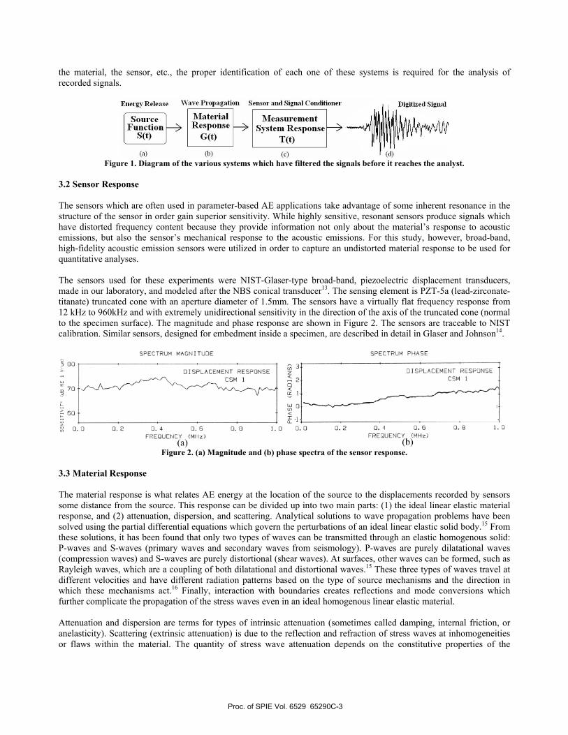
Energy Release Wave Propagation Sensor and Signal Conditioner

MaterialFunction Response

S(t) G(t)

(1))

the material, the sensor, etc., the proper identification of each one of these systems is required for the analysis of recorded signals.

Figure 1. Diagram of the various systems which have filtered the signals before it reaches the analyst.

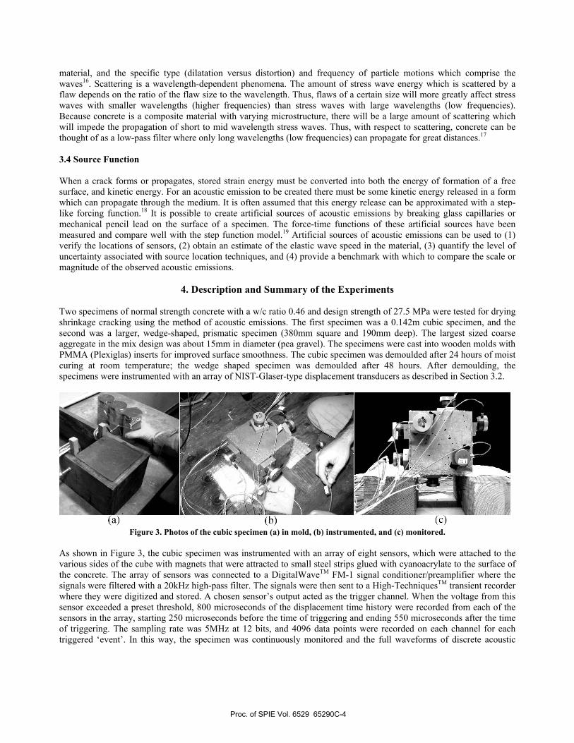
3.2 Sensor Response The sensors which are often used in parameter-based AE applications take advantage of some inherent resonance in the structure of the sensor in order gain superior sensitivity. While highly sensitive, resonant sensors produce signals which have distorted frequency content because they provide information not only about the material’s response to acoustic emissions, but also the sensor’s mechanical response to the acoustic emissions. For this study, however, broad-band, high-fidelity acoustic emission sensors were utilized in order to capture an undistorted material response to be used for quantitative analyses. The sensors used for these experiments were NIST-Glaser-type broad-band, piezoelectric displacement transducers, made in our laboratory, and modeled after the NBS conical transducer13. The sensing element is PZT-5a (lead-zirconate-titanate) truncated cone with an aperture diameter of 1.5mm. The sensors have a virtually flat frequency response from 12 kHz to 960kHz and with extremely unidirectional sensitivity in the direction of the axis of the truncated cone (normal to the specimen surface). The magnitude and phase response are shown in Figure 2. The sensors are traceable to NIST calibration. Similar sensors, designed for embedment inside a specimen, are described in detail in Glaser and Johnson14.

Figure 2. (a) Magnitude and (b) phase spectra of the sensor response.

3.3 Material Response The material response is what relates AE energy at the location of the source to the displacements recorded by sensors some distance from the source. This response can be divided up into two main parts: (1) the ideal linear elastic material response, and (2) attenuation, dispersion, and scattering. Analytical solutions to wave propagation problems have been solved using the partial differential equations which govern the perturbations of an ideal linear elastic solid body.15 From these solutions, it has been found that only two types of waves can be transmitted through an elastic homogenous solid: P-waves and S-waves (primary waves and secondary waves from seismology). P-waves are purely dilatational waves (compression waves) and S-waves are purely distortional (shear waves). At surfaces, other waves can be formed, such as Rayleigh waves, which are a coupling of both dilatational and distortional waves.15 These three types of waves travel at different velocities and have different radiation patterns based on the type of source mechanisms and the direction in which these mechanisms act.16 Finally, interaction with boundaries creates reflections and mode conversions which further complicate the propagation of the stress waves even in an ideal homogenous linear elastic material. Attenuation and dispersion are terms for types of intrinsic attenuation (sometimes called damping, internal friction, or anelasticity). Scattering (extrinsic attenuation) is due to the reflection and refraction of stress waves at inhomogeneities or flaws within the material. The quantity of stress wave attenuation depends on the constitutive properties of the

Proc. of SPIE Vol. 6529 65290C-3

(c)

material, and the specific type (dilatation versus distortion) and frequency of particle motions which comprise the waves16. Scattering is a wavelength-dependent phenomena. The amount of stress wave energy which is scattered by a flaw depends on the ratio of the flaw size to the wavelength. Thus, flaws of a certain size will more greatly affect stress waves with smaller wavelengths (higher frequencies) than stress waves with large wavelengths (low frequencies). Because concrete is a composite material with varying microstructure, there will be a large amount of scattering which will impede the propagation of short to mid wavelength stress waves. Thus, with respect to scattering, concrete can be thought of as a low-pass filter where only long wavelengths (low frequencies) can propagate for great distances.17 3.4 Source Function When a crack forms or propagates, stored strain energy must be converted into both the energy of formation of a free surface, and kinetic energy. For an acoustic emission to be created there must be some kinetic energy released in a form which can propagate through the medium. It is often assumed that this energy release can be approximated with a step-like forcing function.18 It is possible to create artificial sources of acoustic emissions by breaking glass capillaries or mechanical pencil lead on the surface of a specimen. The force-time functions of these artificial sources have been measured and compare well with the step function model.19 Artificial sources of acoustic emissions can be used to (1) verify the locations of sensors, (2) obtain an estimate of the elastic wave speed in the material, (3) quantify the level of uncertainty associated with source location techniques, and (4) provide a benchmark with which to compare the scale or magnitude of the observed acoustic emissions.

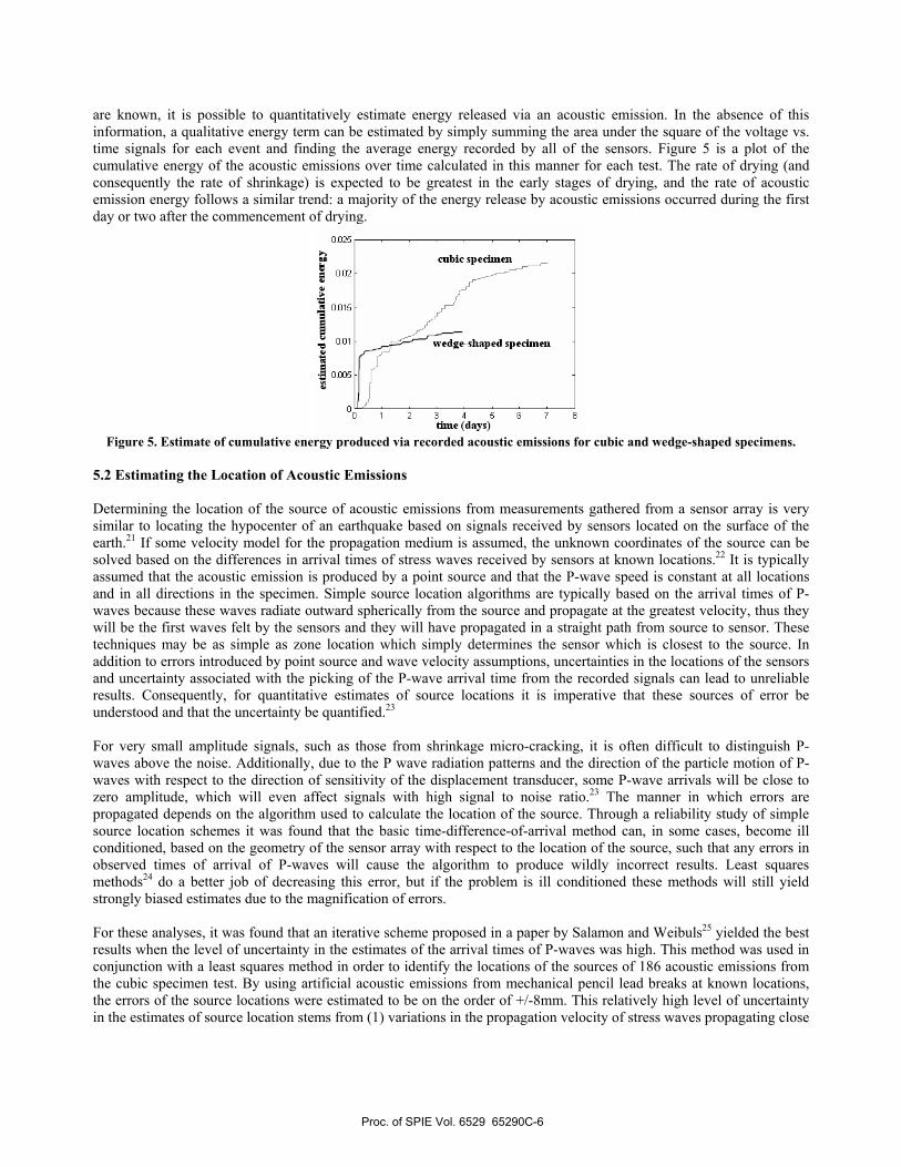
4. Description and Summary of the Experiments Two specimens of normal strength concrete with a w/c ratio 0.46 and design strength of 27.5 MPa were tested for drying shrinkage cracking using the method of acoustic emissions. The first specimen was a 0.142m cubic specimen, and the second was a larger, wedge-shaped, prismatic specimen (380mm square and 190mm deep). The largest sized coarse aggregate in the mix design was about 15mm in diameter (pea gravel). The specimens were cast into wooden molds with PMMA (Plexiglas) inserts for improved surface smoothness. The cubic specimen was demoulded after 24 hours of moist curing at room temperature; the wedge shaped specimen was demoulded after 48 hours. After demoulding, the specimens were instrumented with an array of NIST-Glaser-type displacement transducers as described in Section 3.2.

Figure 3. Photos of the cubic specimen (a) in mold, (b) instrumented, and (c) monitored.

As shown in Figure 3, the cubic specimen was instrumented with an array of eight sensors, which were attached to the various sides of the cube with magnets that were attracted to small steel strips glued with cyanoacrylate to the surface of the concrete. The array of sensors was connected to a DigitalWaveTM FM-1 signal conditioner/preamplifier where the signals were filtered with a 20kHz high-pass filter. The signals were then sent to a High-TechniquesTM transient recorder where they were digitized and stored. A chosen sensor’s output acted as the trigger channel. When the voltage from this sensor exceeded a preset threshold, 800 microseconds of the displacement time history were recorded from each of the sensors in the array, starting 250 microseconds before the time of triggering and ending 550 microseconds after the time of triggering. The sampling rate was 5MHz at 12 bits, and 4096 data points were recorded on each channel for each triggered ‘event’. In this way, the specimen was continuously monitored and the full waveforms of discrete acoustic

Proc. of SPIE Vol. 6529 65290C-4

-

—Il.——'. L(b) (c)

emissions were recorded and saved for offline analysis. Acoustic emissions from the cubic specimen were recorded in this way for one week. Some difficulties were encountered during the testing and when analyzing the results of this cubic specimen test. Firstly, it took two hours of initial setup to attach the sensors properly. Also, due to the low strength of the early age specimen, cracking and spalling of the concrete occurred directly under the steel strips which held the sensors onto the cube, which caused two sensors to lose contact with the specimen approximately thirteen hours after the commencement of drying. This cracking and spalling created acoustic emissions, and it was not until the results were analyzed in detail that the source of these acoustic emissions was identified. Additionally, the cubic specimen was allowed to dry on all sides, making the calculation of the depth of the acoustic emissions a three dimensional problem. Finally, due to the geometry of the cube, there were many reflections present in the recorded acoustic emission signals making it difficult to determine the different phases (P, S, and Rayleigh waves) of the acoustic emission signals. In light of the difficulties encountered during the testing and analysis of the cubic specimen, a second test using a truncated wedge-shaped specimen was designed. The wedge-shaped specimen was instrumented with sixteen sensors which were mounted into a cradle structure shown in Figure 4. The sensor cradle structure eliminated the need for the steel mounting strips and glue. In this test, only the top surface of the wedge shaped specimen was exposed to a low relative humidity (the other surfaces were either painted with wax or covered with plastic wrap) in order to effectively reduce the drying shrinkage to a one-dimensional problem. The larger overall size and wedge geometry was intended to reduce the number of reflections and allow P- and S-wave phases to be better identified in the recorded signals. An additional benefit of the wedge test was that the top surface of the specimen was very smooth which allowed for some of the cracks to be verified visually. Smoothness of the surfaces was achieved by casting the specimen’s drying surface vertically and by the addition of super-plasticizer in the mix design. The wedge-shaped specimen was monitored for four days after the commencement of drying. The main disadvantage of the wedge-shaped specimen was that the larger size increased the length of the travel path from the source to the sensors, which increased the amount attenuation, and decreased the signal to noise ratio.

Figure 4. Photos of wedge-shaped specimen (a) sensor cradle, (b) being demoulded, (c) fully instrumented.

5. Experimental Results and Discussion

5.1 Acoustic Emission Evolution in Time In the cubic specimen, over 6000 acoustic emissions were recorded during the one week monitoring period. Many of these emissions were very small in amplitude and sensed by only one or two sensors. Of these events, only about 300 caused surface displacements with large enough amplitude for signals to be clearly discernable above noise level on more than one or two channels. When testing the wedge-shaped specimen, acoustic emissions were collected for four days totaling about 3000 emissions, only about 100 of which were of significant amplitude. The rate of occurrence of emissions can provide some information about the rate of drying and shrinkage of the concrete, but unfortunately, there is not yet a straight-forward and established relationship between energy measured via acoustic emissions and fracture energy.20 If both the material response and the locations of the sources of all acoustic emissions

Proc. of SPIE Vol. 6529 65290C-5

6.626

002

:1

'0 0.01

0.006

2 3 4 6 6 7 6

dine (days)

are known, it is possible to quantitatively estimate energy released via an acoustic emission. In the absence of this information, a qualitative energy term can be estimated by simply summing the area under the square of the voltage vs. time signals for each event and finding the average energy recorded by all of the sensors. Figure 5 is a plot of the cumulative energy of the acoustic emissions over time calculated in this manner for each test. The rate of drying (and consequently the rate of shrinkage) is expected to be greatest in the early stages of drying, and the rate of acoustic emission energy follows a similar trend: a majority of the energy release by acoustic emissions occurred during the first day or two after the commencement of drying.

Figure 5. Estimate of cumulative energy produced via recorded acoustic emissions for cubic and wedge-shaped specimens.

5.2 Estimating the Location of Acoustic Emissions Determining the location of the source of acoustic emissions from measurements gathered from a sensor array is very similar to locating the hypocenter of an earthquake based on signals received by sensors located on the surface of the earth.21 If some velocity model for the propagation medium is assumed, the unknown coordinates of the source can be solved based on the differences in arrival times of stress waves received by sensors at known locations.22 It is typically assumed that the acoustic emission is produced by a point source and that the P-wave speed is constant at all locations and in all directions in the specimen. Simple source location algorithms are typically based on the arrival times of P-waves because these waves radiate outward spherically from the source and propagate at the greatest velocity, thus they will be the first waves felt by the sensors and they will have propagated in a straight path from source to sensor. These techniques may be as simple as zone location which simply determines the sensor which is closest to the source. In addition to errors introduced by point source and wave velocity assumptions, uncertainties in the locations of the sensors and uncertainty associated with the picking of the P-wave arrival time from the recorded signals can lead to unreliable results. Consequently, for quantitative estimates of source locations it is imperative that these sources of error be understood and that the uncertainty be quantified.23 For very small amplitude signals, such as those from shrinkage micro-cracking, it is often difficult to distinguish P-waves above the noise. Additionally, due to the P wave radiation patterns and the direction of the particle motion of P-waves with respect to the direction of sensitivity of the displacement transducer, some P-wave arrivals will be close to zero amplitude, which will even affect signals with high signal to noise ratio.23 The manner in which errors are propagated depends on the algorithm used to calculate the location of the source. Through a reliability study of simple source location schemes it was found that the basic time-difference-of-arrival method can, in some cases, become ill conditioned, based on the geometry of the sensor array with respect to the location of the source, such that any errors in observed times of arrival of P-waves will cause the algorithm to produce wildly incorrect results. Least squares methods24 do a better job of decreasing this error, but if the problem is ill conditioned these methods will still yield strongly biased estimates due to the magnification of errors. For these analyses, it was found that an iterative scheme proposed in a paper by Salamon and Weibuls25 yielded the best results when the level of uncertainty in the estimates of the arrival times of P-waves was high. This method was used in conjunction with a least squares method in order to identify the locations of the sources of 186 acoustic emissions from the cubic specimen test. By using artificial acoustic emissions from mechanical pencil lead breaks at known locations, the errors of the source locations were estimated to be on the order of +/-8mm. This relatively high level of uncertainty in the estimates of source location stems from (1) variations in the propagation velocity of stress waves propagating close

Proc. of SPIE Vol. 6529 65290C-6

0.1

0.06

0 distamice (ammeters)

016

V distamice (ammeters)

(a) (b) (c) (d)

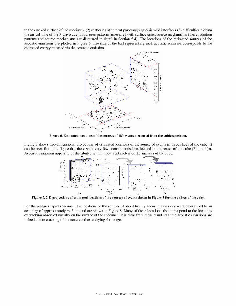
to the cracked surface of the specimen, (2) scattering at cement paste/aggregate/air void interfaces (3) difficulties picking the arrival time of the P-wave due to radiation patterns associated with surface crack source mechanisms (these radiation patterns and source mechanisms are discussed in detail in Section 5.4). The locations of the estimated sources of the acoustic emissions are plotted in Figure 6. The size of the ball representing each acoustic emission corresponds to the estimated energy released via the acoustic emission.

Figure 6. Estimated locations of the sources of 180 events measured from the cubic specimen.

Figure 7 shows two-dimensional projections of estimated locations of the source of events in three slices of the cube. It

can be seen from this figure that there were very few acoustic emissions located in the center of the cube (Figure 6(b). Acoustic emissions appear to be distributed within a few centimeters of the surfaces of the cube.

Figure 7. 2-D projections of estimated locations of the sources of events shown in Figure 5 for three slices of the cube.

For the wedge shaped specimen, the locations of the sources of about twenty acoustic emissions were determined to an accuracy of approximately +/-5mm and are shown in Figure 8. Many of these locations also correspond to the locations of cracking observed visually on the surface of the specimen. It is clear from these results that the acoustic emissions are indeed due to cracking of the concrete due to drying shrinkage.

Proc. of SPIE Vol. 6529 65290C-7

Front View0.05

Top Vio,

-0.15 -0.1 -0.05 0 0.05 0.1 0.15 0.2Xdistance(w)

(a)

45

40

35

E 30

25

20

15

0 5 10 15time (seconds) x ia4 frequency Hz

(a) (b)

Figure 8. Estimated locations of the sources of events (a) front view and (b) top view in the wedge-shaped specimen.

5.3 Frequency Content of the Acoustic Emissions In addition to studying the quantity of acoustic emissions, it is important to study the frequency content of acoustic emissions. This is only possible through the use of broadband sensors with a flat frequency response. The frequency content can aid in the understanding of both the nature of the source and the nature of the medium through which the acoustic waves propagate. All signals shown in this paper are original signals as saved by the transient recorder (no filtering or scaling other than an analogue 20 kHz high-pass filter in the signal conditioner to cut out vibration noise from the laboratory environment).

Figure 9. (a) Displacement time history waveform and (b) corresponding frequency spectra from five sensors monitoring the

same event.

Five signals and their corresponding frequency content are shown in Figure 9(a) and (b) respectively. These signals correspond to the waveforms recorded by five different sensors for the same event. Note that the waveforms and corresponding spectra are offset for clarity and have been displayed in order of time of arrival of the signal (the onset time). Thus, the top signal is from the sensor which first felt the acoustic emission and the bottom signal is from the sensor which last felt the emission. The low-pass filtering effect of concrete can easily be discerned from these signals. The signal with the first onset time (the sensor closest to the source) shows higher frequency content than signals further from the source. Many acoustic emission signals contain frequencies of significant amplitude well above 500 kHz, but concrete strongly attenuates these high frequencies. Fully characterized relationships between attenuation and frequency have been found experimentally.18, 26 In order to quantify the frequency content, some signal parameters were defined: (1) peak frequency and (2) highest frequency above a set amplitude. These parameters were calculated as follows. First the power spectrum was estimated via the Welch method (eight sections, 50% overlap, Hamming window). Then the log of the Welch estimates was smoothed and a common threshold was set for all signals. The smoothed log of the Welch power spectral estimates for

Proc. of SPIE Vol. 6529 65290C-8

MSmwn PS Fr.qurcy4prnxTh. xiS' liSle PS Pr.qoeq. Dktai.. tern the SoS..

e• •e./ • '•• a

• • 25a

• •••• -: 2

oO*!2Yt. 6lime (days) Distaeee tam the surface (re)

(a) (b)

0 ftS 1 15 2 25 3 3.5time (seconds) x io• frequency Hz o5

(a) (b)

45

40

35

3Jm25

16

each of the signals are shown in Figure 9(b), again offset for clarity. The peak frequency was defined to be the frequency at which the highest amplitude was located (the vertical dashed line in Figures 9 and 11) and the highest frequency of significant amplitude was defined to be the highest frequency which exceeded the common threshold slightly higher than the noise level (the vertical dotted line in Figures 9 and 11). These parameters, calculated for each sensor’s record for each of the events, are adequate for individual signals, but an ideal parameter might attempt to describe the acoustic emission independent of the location of the source of the acoustic emission with respect to the sensor array. In an effort to achieve location-independent parameters, median and maximum peak frequency were defined (the median and maximum, respectively, of the peak frequencies calculated from each of the eight sensor traces from events from the cubic specimen). Figure 10(a) is a plot of the maximum peak frequency over time, and Figure 10(b) is a plot of the distance from the surface of the cube to the estimated location of the source of the acoustic emission versus median peak frequency. Again, the size of the circle indicates the estimated energy released via each event.

Figure 10. Frequency parameters plotted against (a) time and (b) depth.

From these plots it can be seen that (1) the high energy acoustic emissions were of a lower frequency, (2) the acoustic emission frequency content was increasing somewhat with time, and (3) there is some correlation between distance from the surface and the frequency content of the acoustic emissions. The first observation is perhaps due to a resonance of the cube which is only excited by lower frequencies. The second observation may be due to the way the attenuation in concrete changes as it cures. The third observation prompted further study of acoustic events whose sources were located further into the interior of the cubic specimen. It was found that many of these “interior” emissions show a large amount of high frequency content centered around one peak frequency and a distinct lack of low frequency components. An example of one of these “interior” emissions is shown in Figure 11.

Figure 11. (a) Displacement time history waveform and (b) corresponding frequency spectra for 5 channels of the same event.

Proc. of SPIE Vol. 6529 65290C-9

C,

0

0 5tine (seconds)x io

(a) (b)

10

tine (setonds)x io-

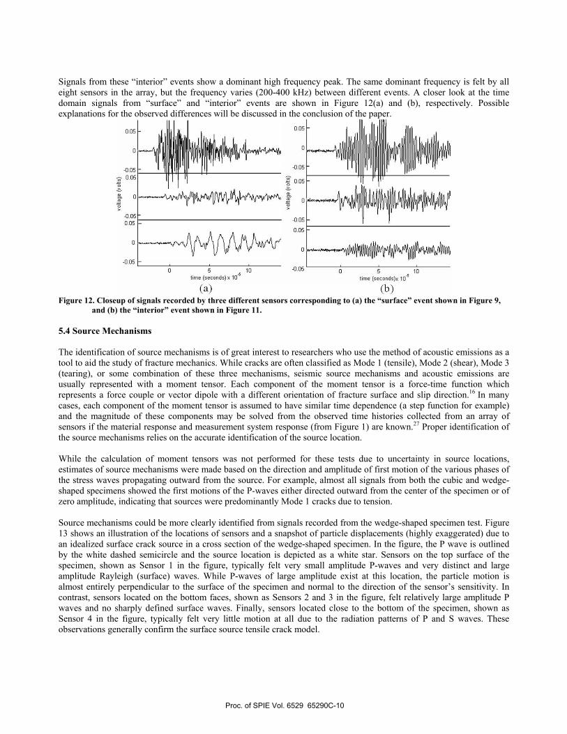
Signals from these “interior” events show a dominant high frequency peak. The same dominant frequency is felt by all eight sensors in the array, but the frequency varies (200-400 kHz) between different events. A closer look at the time domain signals from “surface” and “interior” events are shown in Figure 12(a) and (b), respectively. Possible explanations for the observed differences will be discussed in the conclusion of the paper.

Figure 12. Closeup of signals recorded by three different sensors corresponding to (a) the “surface” event shown in Figure 9,

and (b) the “interior” event shown in Figure 11. 5.4 Source Mechanisms The identification of source mechanisms is of great interest to researchers who use the method of acoustic emissions as a tool to aid the study of fracture mechanics. While cracks are often classified as Mode 1 (tensile), Mode 2 (shear), Mode 3 (tearing), or some combination of these three mechanisms, seismic source mechanisms and acoustic emissions are usually represented with a moment tensor. Each component of the moment tensor is a force-time function which represents a force couple or vector dipole with a different orientation of fracture surface and slip direction.16 In many cases, each component of the moment tensor is assumed to have similar time dependence (a step function for example) and the magnitude of these components may be solved from the observed time histories collected from an array of sensors if the material response and measurement system response (from Figure 1) are known.27 Proper identification of the source mechanisms relies on the accurate identification of the source location. While the calculation of moment tensors was not performed for these tests due to uncertainty in source locations, estimates of source mechanisms were made based on the direction and amplitude of first motion of the various phases of the stress waves propagating outward from the source. For example, almost all signals from both the cubic and wedge-shaped specimens showed the first motions of the P-waves either directed outward from the center of the specimen or of zero amplitude, indicating that sources were predominantly Mode 1 cracks due to tension. Source mechanisms could be more clearly identified from signals recorded from the wedge-shaped specimen test. Figure 13 shows an illustration of the locations of sensors and a snapshot of particle displacements (highly exaggerated) due to an idealized surface crack source in a cross section of the wedge-shaped specimen. In the figure, the P wave is outlined by the white dashed semicircle and the source location is depicted as a white star. Sensors on the top surface of the specimen, shown as Sensor 1 in the figure, typically felt very small amplitude P-waves and very distinct and large amplitude Rayleigh (surface) waves. While P-waves of large amplitude exist at this location, the particle motion is almost entirely perpendicular to the surface of the specimen and normal to the direction of the sensor’s sensitivity. In contrast, sensors located on the bottom faces, shown as Sensors 2 and 3 in the figure, felt relatively large amplitude P waves and no sharply defined surface waves. Finally, sensors located close to the bottom of the specimen, shown as Sensor 4 in the figure, typically felt very little motion at all due to the radiation patterns of P and S waves. These observations generally confirm the surface source tensile crack model.

Proc. of SPIE Vol. 6529 65290C-10

Figure 13. Illustration of radiation patterns from a surface crack model on the surface of the wedge shaped specimen.

6. Conclusion

Two quantitative acoustic emission tests were performed on normal-strength concrete specimens to study the formation of drying shrinkage cracks. The full waveforms of the acoustic emissions were recorded and analyzed. Though more tests need to be performed before many solid conclusions can be made, these two tests have demonstrated many of the strengths and weaknesses of the method of quantitative acoustic emission and can provide some insights into the nature of drying shrinkage cracking and the attenuative properties of concrete. The small specimen size and large area of drying surface on the cubic specimen test produced many acoustic emissions which were all relatively close to the sensors. Thus, a good signal to noise ratio was achieved. On the other hand, reflections from the many surfaces of the cube and internal scattering complicated the energy analyses, and made the determination of different phases (P versus S) extremely difficult. Additionally, the many drying surfaces made a depth analysis much more difficult to carry out. The test on the larger, wedge shaped specimen confirmed the hypothesis that the sources of the acoustic emissions were within a few centimeters of the drying surface, and the smoothness of the drying surface on the wedge allowed shrinkage cracks to be confirmed visually. While the sixteen sensor array geometry decreased the propagation of errors in the source location schemes, signal-to-noise ratio was compromised by the larger distances that the stress waves had to travel before reaching the sensors. Additionally, the sensors’ locations and orientations with respect to radiation patterns made the determination of the P-wave arrival times more difficult, but did confirm surface crack source models to be dominant.

Based on the analyses of the frequency content of the acoustic emissions it is clear that the mechanisms which produce acoustic emissions produce stress waves with significant energy in a broad frequency range of at least 20 kHz to 1000 kHz, but the higher frequencies are greatly attenuated by the inhomogeneous nature of the concrete. It was also noticed that some ‘interior’ events, located somewhat deeper within the specimen, produced displacements at the surface of the specimen that were centered on one specific frequency in the range of 200-400kHz. These high frequency “interior” emissions observed in the cubic specimen were also observed in the wedge shaped specimen, though the location of the sources of these events could not be confirmed. The notably different frequency content of the “interior” events might be explained by some resonant structure near the source of the emission (i.e. the crack tip). If the fracture surface is tortuous enough, the energy released by the emission may cause some structure on the fracture surface to resonate at a certain frequency28, causing the observed high frequency acoustic emission signals. The resonant structure must be located near the source because the same frequency is felt by all sensors for each particular “interior” event, but the central frequency peak of these “interior” acoustic emissions changes between one event and another. The “interior” event frequency phenomenon may facilitate the identification and classification of different types of shrinkage micro-cracks simply from the frequency content of acoustic emissions observed by an array of broad-band, high-fidelity sensors. Acknowledgements

The authors would like to acknowledge Professor Paulo Monteiro for sharing his knowledge of concrete technology and his ideas, enthusiasm, and encouragement throughout the process, and Dr. Lev Stepanov for his help with the mixing and casting of the concrete specimens. This work was funded by NSF-GRF and NSF grants CMS-0624985 (sensor technology).

Proc. of SPIE Vol. 6529 65290C-11

References 1. Grosse, C., Reinhardt, H.-W., and Dahm, T., “Localization and Classification of Fracture Types in Concrete with Quantitative

Acoustic Emission Measurement Techniques,” NDT&E International 30 pp. 223-230, 1996. 2. Kim, K. Y., and Sachse, W., “Characteristics of an acoustic emission source from a thermal crack in glass,” International Journal

of Fracture, 31, pp. 211-231, 1986. 3. Hsu, N. N., and Hardy, S. C. “Experiments in Acoustic Emission Waveform Analysis for Characterization of AE Sources,

Sensors and Structures” American Society of Mechanical Engineers, Applied Mechanics Division, AMD, pp. 85-106, 1978. 4. Grosse, C., Ohtsu, M. (editors), Basics and Applications of Acoustic Emission Testing in Civil Engineering, Springer Publishing,

Heidelberg, ca 2007 (in print). 5. Mehta, P.K. and Monteiro, P.J.M., Concrete: Structure, Properties, and Materials Third Edition, Chapter 4, Prentice-Hall,

Englewood Cliffs, NJ, 2006. 6. Shiotani, T., Bisschop, J., and van Mier, J. G. M. “Temporal and spatial development of drying shrinkage cracking in cement-

based materials,” Engineering Fracture Mechanics, 70, pp. 1509-1525, 2003. 7. Uomoto, T., Kato, H., “Drying Shrinkage of Concrete and Acoustic Emission,” Progress in Acoustic Emission V, Yamaguchi, K.,

Takahashi, H., and Niitsuma, H., pp. 325-330, The Japanese Society for NDI, Sendai, Japan, 1990. 8. Grasley, Z. C., and Lange, D.A., “Modeling Drying Shrinkage Stress Gradients in Concrete,” Cement, Concrete, and Aggregates,

26, pp. 1-8, 2004. 9. Bisschop, J., and van Mier, J. G. M., “Effect of Aggregates on Drying Shrinkage Microcracking in Cement-Based Composites,”

Materials and Structures, 35, pp 453-461, 2002. 10. Ramirez, G., Engelhardt, M., Fowler, T., “On the Endurance Limit of Fiberglass Pipes Using Acoustic Emission,” Journal of

Pressure Vessel Technology, 128, pp. 454-461, 2006. 11. Shah, K., and Lebus, J., “Damage Mechanisms in Stressed Rock from Acoustic Emission,” Journal of Geophysical Research,

100, pp. 15527-15539, 1995. 12. To, A., and Glaser, S., “Full Waveform Inversion of a 3-D Source Inside an Artificial Rock,” Journal of Sound and Vibration,

285, pp. 835-857, 2005. 13. Proctor, T. M. “An improved piezoelectric acoustic emission transducer,” Journal of Acoustic Society of America, 71, pp.1163-

1168, 1982. 14. Glaser, S., Weiss, G., and Johnson, L., “Body Waves Recorded Inside an Elastic Half-space by an Embedded, Wideband

Velocity Sensor,” Journal of Acoustic Society of America, 104, pp. 1404-1412, 1998. 15. Graff, K, Wave Motion in Elastic Solids, Chapters 5 and 6, Oxford University Press, Mineola, NY, 1975. 16. Aki, K., Richards, P. G., Quantitative Seismology: Theory and Methods, Chapter 4, Freeman, San Francisco, 1980. 17. Landis, E., Shah, S., “Frequency-Dependent Stress Wave Attenuation in Cement-Based Materials,” Journal of Engineering

Mechanics, 121, pp. 737-743, 1995. 18. Eitzen, D., Breckenridge, F.,Clough, R., Fuller, E., Hsu, N., and Simmons, J., "Fundamental Developments for Quantitative

Acoustic Emission Measurements," Interim Report NP-2089, prepared for Electric Power Research Institute, 1981. 19. Breckenridge, F., Proctor, T., Hsu, N., Fick, S., Eitzen, D., “Transient Sources for Acoustic Emission Work,” Progress in

Acoustic Emission V, Yamaguchi, K., Takahashi, H., and Niitsuma, H., pp. 20-37, The Japanese Society for NDI, Sendai, Japan, 1990.

20. Landis, E., and Ballion, L., “Experiments to Relate Acoustic Emission Energy to Fracture Energy of Concrete,” Journal of Mechanics, 128, pp. 698-702, 2002.

21. Baron, J., and Ying, S., “Acoustic Emission Source Location,” Nondestructive Testing Handbook Second Edition Vol. 5: Acoustic Emission Testing,Miller, R., and McIntire, P., pp. 136-154, American Society for Nondestructive Testing, 1987.

22. Mahajan, A., and Walworth, M., “3-D position sensing using the differences in the time-of-flights from a wave source to various receivers,” IEEE Transactions on Robotics and Automation, 17, pp. 91-94, 2001.

23. Ge, M., and Kaiser, P. K., “Interpretation of Physical Status of Arrival Picks for Microseismic Source Location,” Bulletin of the Seismological Society of America, 80, pp 1643-1660, 1990.

24. Ohtsu, M., and Ono, K., “AE Source Location and Orientation Determination of Tensile Cracks from Surface Observation,” NDT International, 21, pp. 143-150, 1988.

25. Salamon, M. D. G., and Wiebols, G. A., “Digital Location of Seismic Events by an Underground Network of Seismometers using the Arrival Times of Compressional Waves,” Rock Mechanics, 6, pp. 141-166, 1974.

26. Philippidis, T.P., and Aggelis, D.G. “Experimental Study of Wave Dispersion and Attenuation in Concrete,” Ultrasonics, 43 pp.584-595, 2005.

27. Stump, B., and Johnson, L., “The Determination of Source Properties by the Linear Inversion of Seismograms,” Bulletin of the Seismological Society of America, 67, pp 1489-1502, 1977.

28. Glaser, S., and Nelson, P., “Acoustic Emissions Produced by Discrete Fracture in Rock,” International Journal of Rock Mechanics, Mining Science, and Geomechanics Abstracts, 29, pp. 237-251, 1992.

Proc. of SPIE Vol. 6529 65290C-12