energies

Article

Integrated Traction Control Strategy for DistributedDrive Electric Vehicles with Improvement ofEconomy and Longitudinal Driving Stability

Xudong Zhang * and Dietmar Göhlich

Methods for Product Development and Mechatronics, Technical University of Berlin, 10623 Berlin, Germany;dietmar.goehlich@tu-berlin.de* Correspondence: xudong.zhang@campus.tu-berlin.de

Academic Editor: K.T. ChauReceived: 5 October 2016; Accepted: 3 January 2017; Published: 19 January 2017

Abstract: This paper presents an integrated traction control strategy (ITCS) for distributed driveelectric vehicles. The purpose of the proposed strategy is to improve vehicle economy andlongitudinal driving stability. On high adhesion roads, economy optimization algorithm is appliedto maximize motors efficiency by means of the optimized torque distribution. On low adhesionroads, a sliding mode control (SMC) algorithm is implemented to guarantee the wheel slip ratioaround the optimal slip ratio point to make full use of road adhesion capacity. In order toavoid the disturbance on slip ratio calculation due to the low vehicle speed, wheel rotationalspeed is taken as the control variable. Since the optimal slip ratio varies according to differentroad conditions, Bayesian hypothesis selection is utilized to estimate the road friction coefficient.Additionally, the ITCS is designed for combining the vehicle economy and stability control throughthree traction allocation cases: economy-based traction allocation, pedal self-correcting tractionallocation and inter-axles traction allocation. Finally, simulations are conducted in CarSim andMatlab/Simulink environment. The results show that the proposed strategy effectively reducesvehicle energy consumption, suppresses wheels-skid and enhances the vehicle longitudinal stabilityand dynamic performance.

Keywords: traction control; longitudinal dynamics; electric vehicle; slip ratio control;vehicle economy

1. Introduction

During the past years, due to the energy crisis and environmental concerns, electric vehicles(EVs) have become a fast-growing hotspot [1]. With the improvements on the electric motor andmotor controller technology, many possibilities of power train configurations have been proposed [2,3].One of the latest configurations is known as distributed drive electric vehicles (DDEVs), which employfour motors that are integrated to each wheel and controlled independently. This configuration hasmany advantages such as quick and accurate torque response, easier torque and revolutions per minute(RPM) measurement, and independent control for one single motor, which provides a broad prospectfor vehicle dynamic improvement [4].

Traction control is a significant aspect of vehicle dynamic control and greatly influences vehiclestability, safety and even economy. Therefore, much research has been carried out so far focusing on thisarea [5–9]. Logic threshold control is widely adopted in most of the mature Anti-lock Braking System(ABS) products [10]. However, its low adaptability and precision is also apparent. Fuzzy controlalgorithm has been applied to traction control research in EVs [11]. A maximum torque estimator wasdesigned to achieve the anti-slip control [12]. This method only needs the driving wheels’ torque and

Energies 2017, 10, 126; doi:10.3390/en10010126 www.mdpi.com/journal/energies

Energies 2017, 10, 126 2 of 18

RPM information instead of vehicle body velocity. Besides, model following control (MFC) and slipratio control (SRC) were designed in traction control systems, which were verified through simulationand field test [13]. Due to its robustness, sliding mode control (SMC) has increasingly been applied invehicle traction control [14–16]. Drakunov et al. [17] and Ünsal et al. [18] applied SMC to maintainthe wheel slip at any given value. Wen et al. [19] presented an acceleration slip regulation strategybased on SMC. In this research, slip ratio calculation formula in the form of a state equation is usedfor solving the numerical problem caused by the traditional way. From the perspective of vehicleeconomy, Nam [20] proposed a traction-ability and energy efficiency improvement method usingwheel slip control. However, the energy consumption only led by unnecessary wheel spin can bereduced. Yuan [21] utilized the independent characteristics of traction motors to develop a torquedistribution method for decreasing EV energy. Furthermore, quite a few cost function-based tractionallocation approaches have been carried out. Mokhiamar and Abe [22,23] proposed an allocationalgorithm that minimizes the weighted sum square of the workload of four wheels. However, thiscost function cannot guarantee every tire is fully used. Sometimes, one tire is already nearing its limitwhile the workload of others is relatively low, which impedes the further improvement of vehiclestability. Addressing this drawback, He and Hori [24] and Nishihara and Kumamoto [25] proposeda minimax control allocation that minimizes the utilization of the tire with maximum workload.Yamakawa et al. [26] proposed an optimal torque allocation algorithm using the changeable principleto minimize the dissipation energy produced by the tires on the contact with the ground. It can reducethe tire slippage and transmit motor torques to the ground efficiently. However, due to the largecalculation cost, it is difficult to guarantee the real-time performance of the above algorithms.

Additionally, it is should be noted that the performance of vehicle traction allocation methodsis highly relied on the friction force arising from the contact of tires and the road surface. Therefore,an adequate knowledge of the tire-road friction coefficient is of great importance. Under considerationof the fairly easy and cost-effective implementation, the estimation approaches using vehicle dynamicresponse information has drawn increasing interest recently. In [27], a road friction coefficientestimation method was introduced based on extend Kalman filter and neural network. Simulationresults show that under uncritical driving conditions it has a good performance. Guan et al. [28]presented a maximum friction coefficient estimator by comparing the samples of the estimated valueswith the standard one of each typical road, and using the minimum statistical error as the recognitionprinciple to improve identification robustness.

Most control strategies are incomplete, for they only focus on either stability or energy saving,while taking insufficient account of different road conditions. The major contribution of the presentedintegrated traction control strategy (ITCS) in this paper is given as follows:

(1) Propose an economy-based traction allocation method;(2) Apply Bayes’ theorem to determine the optimal slip ratio under a specific road surface;(3) Design a sliding mode controller to track the desired optimal slip ratio;(4) Build a framework integrating vehicle economy and longitudinal stability control with three

traction allocation cases (economy-based traction allocation, pedal self-correcting tractionallocation and inter-axles traction allocation).

The economy-based traction allocation is developed using an objective function of minimizingpower loss of four electric motors, which does not rely on the complex online computation. It isobtained via an offline optimization procedure and utilized for online allocation by simple interpolation.The low calculation effort makes it easy to implement the algorithm on real vehicles. Subsequently,SMC is used to calculate the torque which can make the tire under the optimal slip ratio point. In orderto avoid the deterioration of direct SRC in the low speed region, the proposed control strategy takeswheel angular velocity as control variable. Finally, the effectiveness of the ITCS for both energy savingand longitudinal stability is validated via the co-simulation of CarSim (Version 9.0.3, Mechanical

Energies 2017, 10, 126 3 of 18

Simulation Corporation, Ann Arbor, MI, USA) and Matlab/Simulink (Version 2012b, MathWorks,Natick, MA, USA).

This paper proceeds as follows. Section 2 presents the DDEV system modeling. In Section 3,the integrated control strategy is developed, which contains economy-based and stability-basedalgorithms. Section 4 performs numerical simulations for different control cases. Finally, someconclusions are drawn in Section 5.

2. System Modeling

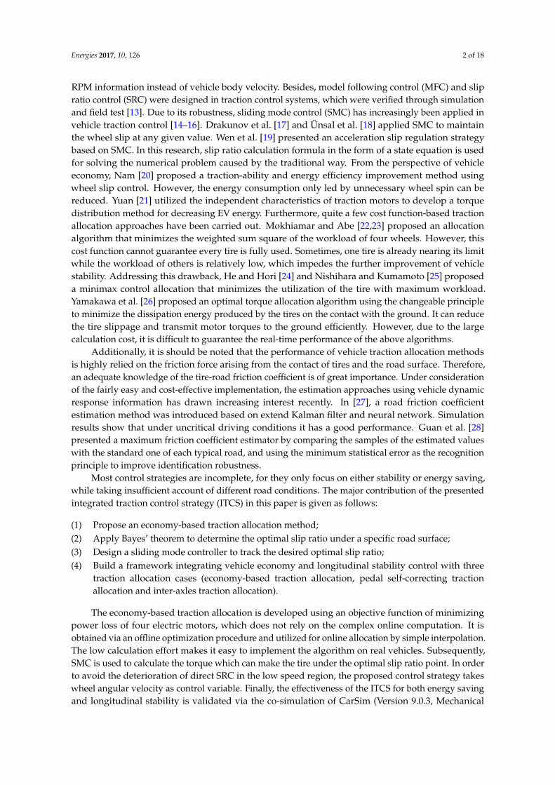
In this section, an EV dynamic model is established using CarSim and Matlab/Simulink, whichis driven by four independently controlled DC motors. The chassis layout is shown in Figure 1.The controller acquires torque and RPM signals from four motors, and then sends them the torquecommand signals.

Energies 2017, 10, 126 3 of 18

This paper proceeds as follows. Section 2 presents the DDEV system modeling. In Section 3, the integrated control strategy is developed, which contains economy-based and stability-based algorithms. Section 4 performs numerical simulations for different control cases. Finally, some conclusions are drawn in Section 5.

2. System Modeling

In this section, an EV dynamic model is established using CarSim and Matlab/Simulink, which is driven by four independently controlled DC motors. The chassis layout is shown in Figure 1. The controller acquires torque and RPM signals from four motors, and then sends them the torque command signals.

Motor Motor

MotorMotor

Torque and RPM Signals

Torque and RPM Signals

Torque and RPM Signals

Torque and RPM Signals

Control Signal Control Signal

Control SignalControl Signal

Integrated Traction Controller

Ft1

Ft3

Ft2

Ft4

Figure 1. Chassis and traction control system layout. RPM: revolutions per minute.

2.1. Vehicle Dynamics Model

A detailed and comprehensive vehicle model must be used to accurately simulate the vehicle response under various maneuvers. Therefore, commercial vehicle dynamics software CarSim is adopted in this study. The embedded vehicle model in CarSim, containing driver model, brakes, steering system, “Pacejka 5.2” tire model, and suspension components, is used to simulate the real vehicle.

2.2. Motor Model

For DDEVs, each wheel is individually driven by a DC motor through a fixed reduction gear. The motor torque external characteristics and efficiency map are shown in Figure 2 [29].

The motor’s torque response can be simplified as first-order inertia as the following equation:

1cmdi

iT

Tts

=+

(1)

where Ti is the motor torque output; Tcmdi is the torque command signal; and t is the time constant. Since motor power is the function of motor efficiency, rotational speed and torque output,

based on the efficiency map in Figure 2, the motor power can be easily calculated as:

Figure 1. Chassis and traction control system layout. RPM: revolutions per minute.

2.1. Vehicle Dynamics Model

A detailed and comprehensive vehicle model must be used to accurately simulate the vehicleresponse under various maneuvers. Therefore, commercial vehicle dynamics software CarSim isadopted in this study. The embedded vehicle model in CarSim, containing driver model, brakes,steering system, “Pacejka 5.2” tire model, and suspension components, is used to simulate thereal vehicle.

2.2. Motor Model

For DDEVs, each wheel is individually driven by a DC motor through a fixed reduction gear.The motor torque external characteristics and efficiency map are shown in Figure 2 [29].

The motor’s torque response can be simplified as first-order inertia as the following equation:

Ti =Tcmdits + 1

(1)

where Ti is the motor torque output; Tcmdi is the torque command signal; and t is the time constant.

Energies 2017, 10, 126 4 of 18

Since motor power is the function of motor efficiency, rotational speed and torque output, basedon the efficiency map in Figure 2, the motor power can be easily calculated as:

Pi =ni · Tiηi(Ti, ni)

(2)

where Pi and ni denote the motor power and rotational speed. ηi is the efficiency for four motors whichcan be obtained from Figure 2 with current torque and RPM signals.

Energies 2017, 10, 126 4 of 18

( )η ,i i

ii i i

n TP

T n

⋅= (2)

where Pi and ni denote the motor power and rotational speed. η i is the efficiency for four motors which can be obtained from Figure 2 with current torque and RPM signals.

Figure 2. Motor torque external characteristics and efficiency map.

For each wheel, the driving equation is given as:

ωi i tiI T beta F r⋅ = ⋅ − ⋅ (3)

where Ii is the wheel inertia; r is the wheel radius; beta is the reducer ratio; and Fti is wheel longitudinal force.

3. Integrated Control Strategy Design

Under the premise of ensuring vehicle stability, its economy performance needs to be improved as much as possible, for EVs are developed to be a solution to the energy crisis. In order to achieve that, two traction control algorithms are discussed in the following subsections. One is for economy promotion, and the other is aimed at guaranteeing the vehicle longitudinal stability. Finally, to combine them together through three traction allocation cases, the integrated control strategy is introduced and its schematic is illustrated in Figure 3.

Economy-based Traction Allocation

Pedal Self-correcting Traction Allocation

Integrated Traction Control Strategy

Con

trol

Cas

e Se

lect

ion

T1

T2

T3

T4

ω1

ω2

ω3

ω4Inter-axles Traction Allocation

Figure 3. Schematic of the proposed integrated control strategy.

Figure 2. Motor torque external characteristics and efficiency map.

For each wheel, the driving equation is given as:

Ii ·.ω = Ti · beta− Fti · r (3)

where Ii is the wheel inertia; r is the wheel radius; beta is the reducer ratio; and Fti is wheellongitudinal force.

3. Integrated Control Strategy Design

Under the premise of ensuring vehicle stability, its economy performance needs to be improvedas much as possible, for EVs are developed to be a solution to the energy crisis. In order to achievethat, two traction control algorithms are discussed in the following subsections. One is for economypromotion, and the other is aimed at guaranteeing the vehicle longitudinal stability. Finally, to combinethem together through three traction allocation cases, the integrated control strategy is introduced andits schematic is illustrated in Figure 3.

Energies 2017, 10, 126 4 of 18

( )η ,i i

ii i i

n TP

T n

⋅= (2)

where Pi and ni denote the motor power and rotational speed. η i is the efficiency for four motors which can be obtained from Figure 2 with current torque and RPM signals.

Figure 2. Motor torque external characteristics and efficiency map.

For each wheel, the driving equation is given as:

ωi i tiI T beta F r⋅ = ⋅ − ⋅ (3)

where Ii is the wheel inertia; r is the wheel radius; beta is the reducer ratio; and Fti is wheel longitudinal force.

3. Integrated Control Strategy Design

Under the premise of ensuring vehicle stability, its economy performance needs to be improved as much as possible, for EVs are developed to be a solution to the energy crisis. In order to achieve that, two traction control algorithms are discussed in the following subsections. One is for economy promotion, and the other is aimed at guaranteeing the vehicle longitudinal stability. Finally, to combine them together through three traction allocation cases, the integrated control strategy is introduced and its schematic is illustrated in Figure 3.

Economy-based Traction Allocation

Pedal Self-correcting Traction Allocation

Integrated Traction Control Strategy

Con

trol

Cas

e Se

lect

ion

T1

T2

T3

T4

ω1

ω2

ω3

ω4Inter-axles Traction Allocation

Figure 3. Schematic of the proposed integrated control strategy. Figure 3. Schematic of the proposed integrated control strategy.

Energies 2017, 10, 126 5 of 18

3.1. Economy Control

3.1.1. Objective Functions Establishment

The relationship among the motor’s torque, RPM and efficiency is shown in Figure 2. It can beseen that the motor efficiency is quite distinguishing in different working regions and especially whenit works in the low speed or low torque output region, the motor has poor efficiency.

(1) When a vehicle is running at high speed and the driving torque is distributed equally to thefour wheels in the most common way, according to Figure 2, for one single motor it must bepoorly efficient because of its low torque output. Oppositely, if we use front-wheel-drive (FWD)or rear-wheel-drive (RWD) instead of four-wheel-drive (4WD), then the motor torque output willincrease about twice the original. That means the motor works more efficiently.

(2) When a vehicle starts accelerating with high torque, the driving torque is only distributed to thefront or rear wheels, which is also a very low efficiency allocation way. According to Figure 2, inthis case, 4WD is an obviously better pattern.

According to the above qualitative analysis, a single distribution pattern cannot meet the actualvehicle economy demand. If the driving torque can be real-time distributed among four motorsaccording to motor operating conditions, then motors efficiency will be improved [30]. The followingobjective functions are established:

minJd =4

∑i=1−4

Pi =4

∑i=1−4

ni · Tiηi(Ti, ni)

(4)

The objective functions should satisfy the following equality constraints and inequality constraints,the desired driving torque Td, understeer characteristics, the motor properties, and a few assumptions.

s.t.4

∑i=1−4

Ti = Td (5)

T1 + T3 ≥ T2 + T4 (6)

|Ti| ≤ |Tmotor| (7)

where Tmotor is the motor maximum torque.In order to simplify the calculation, a few assumptions are listed here.

(1) The slip ratio and rotational speed difference of each wheel is quite small.(2) The torque output is identical if the motors are on the same axle.

Despite its simplification, these assumptions are still justified, since only longitudinal dynamic isdiscussed in this study and economy control will be activated only when the controller is fully surethat the car runs stable.

The assumptions can be formulated as:

T1 = T3 = Tf /2 = p · Td/2 (8)

T2 = T4 = Tr/2 = (1− p) · Td/2 (9)

n = beta · ur· 30π

(10)

where p ∈ [0.5, 1] is economy distribution coefficient; Tf is the front axle driving torque; Tr is the rearaxle driving torque; and u is the vehicle longitudinal velocity.

Energies 2017, 10, 126 6 of 18

Then, the final economy objective function is obtained:

Jd = n ·

p · Td

η[

p·Td2 , n

] +(1− p) · Td

η[(1−p)·Td

2 , n] (11)

3.1.2. Solutions to Objective Functions

In this paper, genetic algorithm is applied to solve these discontinuous objective functions. It caneffectively prevent local optimization and find the solutions accurately and rapidly.

The objective function solution p is given as a two-dimensional lookup table with current desireddriving torque and motor rotational speed, which can avoid numerous online calculations and meetsystem real-time requirements. The economy distribution coefficient p is shown in Figure 4.

Energies 2017, 10, 126 6 of 18

( )( )

1

1η , η ,

2 2

p T p Td dJ nd p T p Td dn n

⋅ − ⋅ = ⋅ + ⋅ − ⋅

(11)

3.1.2. Solutions to Objective Functions

In this paper, genetic algorithm is applied to solve these discontinuous objective functions. It can effectively prevent local optimization and find the solutions accurately and rapidly.

The objective function solution p is given as a two-dimensional lookup table with current desired driving torque and motor rotational speed, which can avoid numerous online calculations and meet system real-time requirements. The economy distribution coefficient p is shown in Figure 4.

Figure 4. Economy distribution coefficient map.

For one single control cycle, the driver desired torque Td and motor rotational speed n are taken as the input parameters. Torque distribution coefficient is obtained as the output value through look-up table and interpolation.

Some conclusions can be drawn from the proportional distribution coefficient map:

(1) On different working conditions, in order to achieve the high efficiency performance, different distribution coefficients are demanded;

(2) In the low torque region, all the distribution coefficients equal 1, which shows that the FWD is applied as a better pattern when the torque demand is relatively small;

(3) In medium and high torque region, the distribution coefficients are 0.5 or slightly greater than 0.5, which shows that 4WD can achieve higher efficiency;

(4) In the low speed region, there is almost no transitional area between the regions of distribution coefficient of 0.5 and 1. That is because the isoefficiency curves are very dense in this area, which will lead to the sudden change in distribution coefficient map.

3.2. Stability Control

3.2.1. Optimal Slip Ratio

Tires at optimal slip ratio can make full use of the road driving ability. For actual vehicles and roads, optimal slip ratio is not a constant value. It changes due to the change of road conditions and its variation range is as much as 20%. Thus, it is significant to find the optimal slip ratio in real time. Some papers simply set the optimal slip as a fixed point, such as the average value of optimal slip

02000

40006000

0

200

400

0.5

0.6

0.7

0.8

0.9

1

RPM(r/min)Torque(N*m)

Dis

trib

utio

n co

effic

ient

Figure 4. Economy distribution coefficient map.

For one single control cycle, the driver desired torque Td and motor rotational speed n are taken asthe input parameters. Torque distribution coefficient is obtained as the output value through look-uptable and interpolation.

Some conclusions can be drawn from the proportional distribution coefficient map:

(1) On different working conditions, in order to achieve the high efficiency performance, differentdistribution coefficients are demanded;

(2) In the low torque region, all the distribution coefficients equal 1, which shows that the FWD isapplied as a better pattern when the torque demand is relatively small;

(3) In medium and high torque region, the distribution coefficients are 0.5 or slightly greater than 0.5,which shows that 4WD can achieve higher efficiency;

(4) In the low speed region, there is almost no transitional area between the regions of distributioncoefficient of 0.5 and 1. That is because the isoefficiency curves are very dense in this area,which will lead to the sudden change in distribution coefficient map.

3.2. Stability Control

3.2.1. Optimal Slip Ratio

Tires at optimal slip ratio can make full use of the road driving ability. For actual vehicles androads, optimal slip ratio is not a constant value. It changes due to the change of road conditions and

Energies 2017, 10, 126 7 of 18

its variation range is as much as 20%. Thus, it is significant to find the optimal slip ratio in real time.Some papers simply set the optimal slip as a fixed point, such as the average value of optimal slipratio on all kinds of roads or the optimal slip ratio in statistics. However, either way, these optimal slipratios cannot ensure the optimum state of traction control system.

In this paper, the road conditions are classified into 10 levels, which are corresponding maximumtire/road friction coefficient µ from 0.1 to 1 (0.1, 0.2, 0.3, 0.4, 0.5, 0.6, 0.7, 0.8, 0.9 and 1). According tothe Tire test module in CarSim, tire characteristic simulation is carried out and the optimal slip ratiounder different road friction coefficients is listed as Table 1.

Table 1. Road friction coefficient and the corresponding optimal slip ratio.

Road Level 1 2 3 4 5 6 7 8 9 10

Friction coefficient 1 0.9 0.8 0.7 0.6 0.5 0.4 0.3 0.2 0.1Optimal slip ratio % 19 17 15 13.2 11.3 9.4 7.6 5.6 3.7 1.9

3.2.2. Road Friction Coefficient Estimation

In Table 1, it can be seen that there is a one-to-one correspondence between road friction coefficientand the optimal slip ratio. In this paper, a Bayes’ theorem-based iteration algorithm is applied toestimate the road adhesion coefficient [31].

At sampling time tk, the estimated wheel slip ratio, longitudinal tire force and vertical force areexpressed as λ, Ft and Fz, respectively, which could be identified by a dual extended Kalman filter(DEKF) proposed by Wenzel et al. [32]. Here, the estimated normalized driving factor is given as:

ϕk =Ft

Fz(12)

According to the tire model, with λ another normalized driving factor is obtained, denoted byϕi,k,where i stands for the road level from 1 to 10. The error between ϕk and ϕi,k is calculated as follows:

ei,k =|ϕi,k − ϕk|

ϕk, i = 1, 2, 3, . . . , 10 (13)

The condition possibility of ϕk corresponding to different road levels is equivalent to theprobability distribution of error ei,k. The following likelihood function is obtained:

pk[ϕk|µi] =1√2πσ

e−e2i,k

2σ2 , i = 1, 2, 3, . . . , 10 (14)

where σ is the standard deviation.The prior probability that the road/tire coefficient equals to µi is Pk(µi). Then, we have:

∑10i=1 Pk(µi) = 1 (15)

On basis of Bayes’ rule, under the condition that the estimated normalized driving factor is ϕk,the posterior probability of the road/tire coefficient is expressed as follows:

Qk[µi|ϕk] =pk[ϕk|µi]Pk[µi]

∑10i=1 pk[ϕk|µi]Pk[µi]

, i = 1, 2, 3, . . . , 10 (16)

Energies 2017, 10, 126 8 of 18

Then, at sampling time tk, the road/tire friction coefficient could be estimated as:

µk = ∑10i=1 Qk[µi|ϕk]µi (17)

The next sampling time t = tk+1, set Pk+1[µi] = Qk[µi|ϕk], repeating the above above-mentionedprocess, the online road level estimation can be achieved. Finally, the optimal slip ratio is also derivedaccording to the estimated friction coefficient.

3.2.3. Optimal Slip Ratio Control

In driving condition, wheel slip ratio is defined as:

λ =ω · r− u

u(18)

It is apparent that in the low speed region, slip ratio in this equation is sensitive to the vehiclespeed, which may leads to a large disturbance of the slip ratio calculation. Addressing this issue, inthis paper, optimal SRC is achieved via the wheel rotational speed.

ωo =u

(1− λo) · r(19)

where λo is the optimal slip ratio andωo denotes the corresponding rotational speed.Then, a sliding mode controller is developed to make the actual wheel rotational speedω track

the optimal valueωo described above. Then, the track error is defined as:

e = ω−ωo (20)

Define a switching function s as follows:

s = e + c∫

e dt (21)

where c is the constant switching function coefficient. Equation (21) represents the designed slidingsurface. In this paper, exponential reaching law is selected and given as:

.s = −ks− εsgn(s) (22)

where k is the strictly positive constant gain and ε is reaching velocity factor. By adjusting theparameters k and ε of the exponential reaching law, we can guarantee the dynamic quality of theprocess of sliding mode reaching and weaken the chattering existed in the SMC method.

Taking the derivative of Equation (21) and substituting into Equation (22) gives:

− ks− εsgn(s) =.e + ce (23)

Then, the SMC law is derived by substituting Equation (3) into Equation (23):

To =−[εsgn(s) + ks + c(ω−ωo)] · I + Ft · r

beta(24)

where To is defined as the torque which can make the tire reach the optimal slip ratio.Additionally, the chattering of sliding mode controller is reduced using the following saturation

function instead of sign function:

sat(s/Φ) =

{s/Φ |s| ≤ Φsgn(s) |s| > Φ

(25)

Energies 2017, 10, 126 9 of 18

where Φ is a positive constant.

3.3. Integrated Control Strategy

The integrated control strategy aiming at the economy optimization and stability control isproposed based on the analysis of the driver desired torque, motor output and road adhesion capability.

The control system diagram is shown in Figure 5. As can be seen, the proposed integrated controlstrategy involves three parts: road level estimation, control input and control case selection.

Energies 2017, 10, 126 9 of 18

The control system diagram is shown in Figure 5. As can be seen, the proposed integrated

control strategy involves three parts: road level estimation, control input and control case selection.

Figure 5. Structure of the integrated control strategy (∀: for all; ˄: or; ∃: there exist).

Essentially speaking, road level estimation is to utilize Bayesian hypothesis selection to

estimate the optimal slip ratio in real time. The results are then transferred to control input and case

selection.

Control input is a part for signals acquisition and integration. These signals consist of driver

desired torque signal, motor RPM signals, and reference wheel rotational speed. All of them will be

shared with road level estimation and control case selection.

As for control case selection, it is the core of the proposed strategy. Three cases are designed

and given as follows:

Case 1: economy-based traction allocation. Activation condition: for all ωi ≤ ωoi, corresponding

to high adhesion road. When a vehicle is traveling on this kind of surface, the traction for each tire

offered by the road is greater than the actual motor output, which means in this situation no tire skid

issues exists. Therefore, economy-based traction allocation is activated. The torque output for front

and rear axle:

Tf = p × Td (26)

Tr = (1 − p) × Td (27)

Case 2: pedal self-correcting traction allocation. Activation condition: for all ωi > ωoi,

corresponding to low adhesion road. When a vehicle is driving on a low adhesion road like snow

Road condition

estimation

Reference rotational speed of each wheel

Driver desired torque Td

Current motor Stateω1 ω2 ω3 ω4

Reference rotational speed of each wheel

ωo1 ωo2 ωo3 ωo4

Inter-Axles Torque Allocation

Pedal Self-Correcting Torque Allocation

Efficiency-Based Torque Allocation

∃ ωi>ωoiω1,3≤0.95ωo1,3

ω2,4≤0.95ωo2,4∃ωi≤0.95ωoi

Case reselect

Y Y Y

N

Case 1 (∀ωi≤ωoi) Case 2 (∀ωi>ωoi)Case 3

(ω1,3>ωo1,3∧ω2,4≤ωo2,4)(ω1,3≤ωo1,3∧ω2,4>ωo2,4)

N N

Control input

Control case select

Road level estimation

T1 T2 T3 T4T1 T2 T3 T4 T1 T2 T3 T4

Figure 5. Structure of the integrated control strategy (∀: for all; ∧: or; ∃: there exist).

Essentially speaking, road level estimation is to utilize Bayesian hypothesis selection to estimatethe optimal slip ratio in real time. The results are then transferred to control input and case selection.

Control input is a part for signals acquisition and integration. These signals consist of driverdesired torque signal, motor RPM signals, and reference wheel rotational speed. All of them will beshared with road level estimation and control case selection.

As for control case selection, it is the core of the proposed strategy. Three cases are designed andgiven as follows:

Case 1: economy-based traction allocation. Activation condition: for allωi ≤ ωoi, correspondingto high adhesion road. When a vehicle is traveling on this kind of surface, the traction for each tireoffered by the road is greater than the actual motor output, which means in this situation no tire skid

Energies 2017, 10, 126 10 of 18

issues exists. Therefore, economy-based traction allocation is activated. The torque output for frontand rear axle:

Tf = p × Td (26)

Tr = (1 − p) × Td (27)

Case 2: pedal self-correcting traction allocation. Activation condition: for all ωi > ωoi,corresponding to low adhesion road. When a vehicle is driving on a low adhesion road like snow roador even quick starts and stops on wet cement road, sometimes the road adhesion capacity cannot meetthe driver’s torque request, which will lead to tire’s unstable skid. In order to avoid this situation, theacceleration pedal coefficient must be adjusted to a reasonable region to guarantee vehicle stability.Pedal self-correcting traction allocation is designed to keep actual wheel slip ratio at the optimal slipratio point, to make the most of the road friction and to meet the driver desired torque as far as possible.In this case, the torque output for front and rear axle are given as:

Tf =−[εsgn(s) + ks + c(ω f −ωo f )] · I + Ft f · r

beta(28)

Tr =−[εsgn(s) + ks + c(ωr −ωor)] · I + Ftr · r

beta(29)

Case 3: inter-axles traction allocation. Activation condition: front wheels or rear wheels startto skid. It corresponds to intermediate adhesion road. In addition to high and low adhesion road,sometimes even though the total road adhesion is more than the driver desired torque, if the car isrunning on a joint road, the friction coefficient for front and rear wheels is different. Alternatively, dueto the vehicle load distribution, the wheel with lower vertical load can only be applied with relativelysmall traction. Otherwise, it may lead to a seriously tire skid. Conversely, for the wheel with largervertical load, it is necessary to moderately increase its motor torque output to make full use of the roadcapacity. For example, if the slip phenomenon occurs on front axle, the torque output for front andrear axle are:

Tf =−[εsgn(s) + ks + c(ω f −ωo f )] · I + Ft f · r

beta(30)

Tr = Td − Tf (31)

By comparing different signals, a suitable control case will be activated and kept operating untilthe vehicle running condition changes.

Besides, due to the external disturbance or signal noise, there may be fluctuation during wheelspeed control. In order to avoid case switching frequently, Case 1 will be terminated under thecondition of there exitsωi >ωoi which lasts for five motor control cycles (50 ms) and Cases 2 and 3 willbe terminated when the rotational speed of the controlled wheel is smaller than 95% of the referencespeed and lasts for five motor control cycles (50 ms).

4. Simulation Results and Analysis

The purpose of this section is to verify the proposed ITCS using computer simulations. Firstly,three control cases are evaluated separately in different simulation conditions. Then, variable roadand desired torque conditions are applied to validate the integrated control strategy. The vehicleparameters are listed in the Table 2.

Energies 2017, 10, 126 11 of 18

Table 2. Vehicle parameters.

Parameters Values Unit

Vehicle mass 1280 kgVehicle inertia about Z axis 2460 kg·m2

Distance of center of gravity (c.g.) from front axle 1.2 mDistance of c.g. from rear axle 1.3 m

Frontal projected area 2.1 m2

Wheels track 1.5 mair resistance coefficient 0.32 -

Reducer ratio 3.5 -Reducer efficiency 0.9 -

Tire radius 0.3 mHeight of the sprung mass c.g. 0.5 m

Wheel rotational inertia 2.2 kg·m2

4.1. Simulation on Case 1: Economy-Based Traction Allocation

This economy evaluation is carried out according to the New European Driving Cycle (NEDC).The four-wheel even torque drive (4WETD) and FWD are chosen to compare with the proposed ITCS.Figures 6 and 7 show the simulation results.

Energies 2017, 10, 126 11 of 18

4.1. Simulation on Case 1: Economy-Based Traction Allocation

This economy evaluation is carried out according to the New European Driving Cycle (NEDC). The four-wheel even torque drive (4WETD) and FWD are chosen to compare with the proposed ITCS. Figures 6 and 7 show the simulation results.

Figure 6. Efficiency and its improvement rate: (a) traction efficiency of different allocation approaches; and (b) efficiency improvement.

It can be seen from Figure 6 that vehicle traction efficiency is significantly improved after adopting ITCS. In some conditions, the improvement rate even reaches around 12%. Besides, as Figure 7 shows, the ITCS also achieves lower thermal loss than the others, which can reduce motor’s heat load and prolong its service life.

Figure 7. Heat loss and its reduction rate: (a) heat loss of different allocation approaches; and (b) heat loss reduction.

0 200 400 600 800 1000 1200

0.7

0.8

0.9

1

time [s]

trac

tion

effic

ienc

y [-

]

(a)

4WEDT FWD ITCS

0 200 400 600 800 1000 12000

5

10

15

20

time [s]

effic

ienc

y im

prov

emen

t [%

]

(b)

4WEDT/ITCS FWD/ITCS

0 200 400 600 800 1000 12000

200

400

600

800

time [s]

heat

loss

[kJ

]

(a)

4WEDT FWD ITCS

0 200 400 600 800 1000 12000

10

20

30

40

time [s]

heat

loss

red

uctio

n [%

]

(b)

4WEDT/ITCS FWD/ITCS

Figure 6. Efficiency and its improvement rate: (a) traction efficiency of different allocation approaches;and (b) efficiency improvement.

It can be seen from Figure 6 that vehicle traction efficiency is significantly improved after adoptingITCS. In some conditions, the improvement rate even reaches around 12%. Besides, as Figure 7 shows,the ITCS also achieves lower thermal loss than the others, which can reduce motor’s heat load andprolong its service life.

Energies 2017, 10, 126 12 of 18

Energies 2017, 10, 126 11 of 18

4.1. Simulation on Case 1: Economy-Based Traction Allocation

This economy evaluation is carried out according to the New European Driving Cycle (NEDC). The four-wheel even torque drive (4WETD) and FWD are chosen to compare with the proposed ITCS. Figures 6 and 7 show the simulation results.

Figure 6. Efficiency and its improvement rate: (a) traction efficiency of different allocation approaches; and (b) efficiency improvement.

It can be seen from Figure 6 that vehicle traction efficiency is significantly improved after adopting ITCS. In some conditions, the improvement rate even reaches around 12%. Besides, as Figure 7 shows, the ITCS also achieves lower thermal loss than the others, which can reduce motor’s heat load and prolong its service life.

Figure 7. Heat loss and its reduction rate: (a) heat loss of different allocation approaches; and (b) heat loss reduction.

0 200 400 600 800 1000 1200

0.7

0.8

0.9

1

time [s]

trac

tion

effic

ienc

y [-

]

(a)

4WEDT FWD ITCS

0 200 400 600 800 1000 12000

5

10

15

20

time [s]

effic

ienc

y im

prov

emen

t [%

]

(b)

4WEDT/ITCS FWD/ITCS

0 200 400 600 800 1000 12000

200

400

600

800

time [s]

heat

loss

[kJ

]

(a)

4WEDT FWD ITCS

0 200 400 600 800 1000 12000

10

20

30

40

time [s]

heat

loss

red

uctio

n [%

]

(b)

4WEDT/ITCS FWD/ITCS

Figure 7. Heat loss and its reduction rate: (a) heat loss of different allocation approaches; and (b) heatloss reduction.

Table 3 lists the simulation results of economy improvement and equivalent weight reductionin each driving cycle stage. The highest energy saving occurs in high speed stage. ITCS decreases4.632% energy consumption compared with 4WETD. Lowest energy saving, 0.134%, also occurs inhigh speed stage but it is relative to FWD. As for the whole driving cycle, ITCS can decrease 3.584%and 1.992% energy consumption, respectively, by comparison to 4WETD and FWD. If we use weightto measure the energy saving effect, it means 47.02 kg and 26.11 kg weight reduction equivalently,which is difficult to achieve in engineering design phase.

Table 3. Improvement analysis among different traction allocation strategies. ITCS: integrated tractioncontrol strategy; 4WETD: four-wheel even torque drive; and FWD: front-wheel-drive.

Cycle StageEnergy Consumption (kJ)

Energy Saving Equivalent Weight Reduction (kg)Traditional Allocation ITCS

Low Speed 4WETD 1406.361373.35

2.347% 30.91 kgFWD 1431.29 4.048% 53.04 kg

High Speed 4WETD 1658.661581.82

4.632% 60.69 kgFWD 1583.95 0.134% 3.8 kg

Whole Cycle 4WETD 3065.022995.17

3.584% 47.02 kgFWD 3015.24 1.992% 26.11 kg

4.2. Simulation on Case 2: Pedal Self-Correcting Traction Allocation

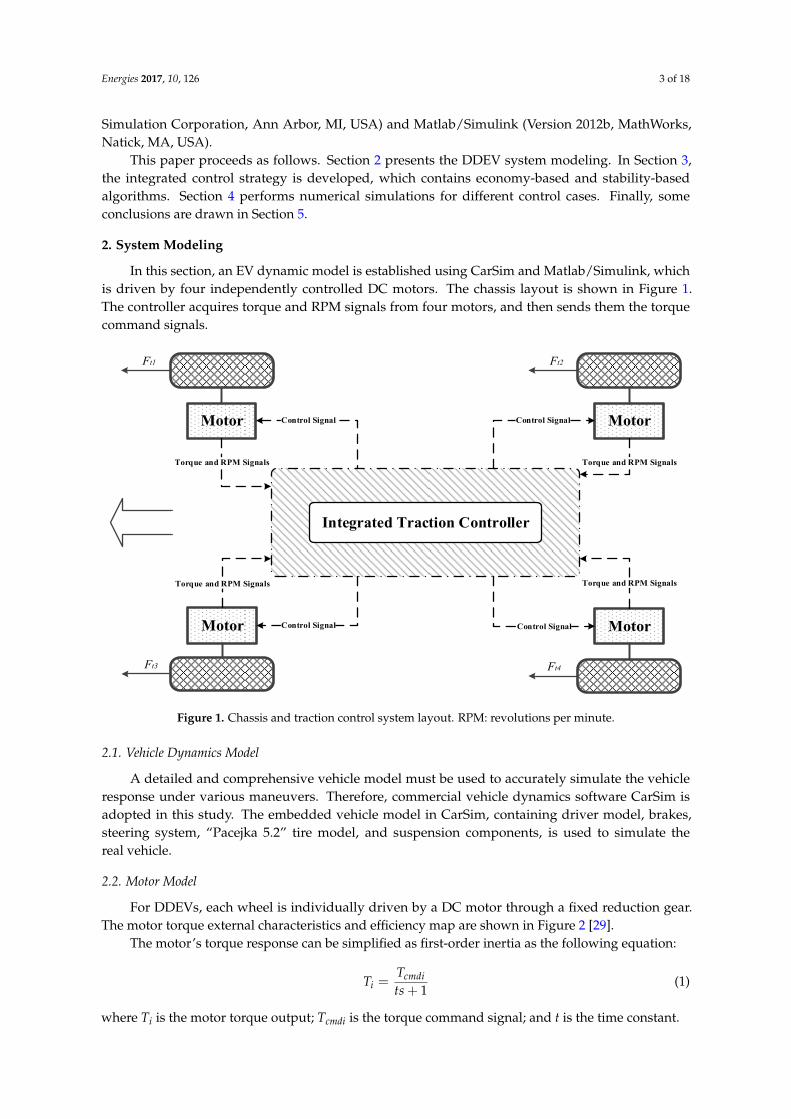
When simulated, the pedal signal is set at 70% opening. The tire/road friction coefficient equals0.2 corresponding to wet hard packed snow road. Figures 8 and 9 show the results of the simulationexperiment between pedal self-correcting traction allocation (with control) and even traction allocation(without control). During the whole time history, it is clear that the vehicle with pedal self-correctingtraction allocation obtains better acceleration performance as shown in Figure 8a. Besides, it can beknown from Figure 8d, the tires without control seriously slip, since the driver desired traction isgreater than that provided by the road. By contrast, in Figures 8b, 9 and 10c, we can see that whenthe pedal self-correcting control is adopted, the accelerator pedal position signal adjusts rapidly from

Energies 2017, 10, 126 13 of 18

70% opening to 65%, the torque assigned to four wheels reduces immediately and then the slip ratio ofeach wheel is kept around the optimal point 3.7%.

Energies 2017, 10, 126 12 of 18

Table 3 lists the simulation results of economy improvement and equivalent weight reduction in each driving cycle stage. The highest energy saving occurs in high speed stage. ITCS decreases 4.632% energy consumption compared with 4WETD. Lowest energy saving, 0.134%, also occurs in high speed stage but it is relative to FWD. As for the whole driving cycle, ITCS can decrease 3.584% and 1.992% energy consumption, respectively, by comparison to 4WETD and FWD. If we use weight to measure the energy saving effect, it means 47.02 kg and 26.11 kg weight reduction equivalently, which is difficult to achieve in engineering design phase.

Table 3. Improvement analysis among different traction allocation strategies. ITCS: integrated traction control strategy; 4WETD: four-wheel even torque drive; and FWD: front-wheel-drive.

Cycle Stage Energy Consumption (kJ)

Energy Saving Equivalent Weight Reduction (kg) Traditional Allocation ITCS

Low Speed 4WETD 1406.36

1373.35 2.347% 30.91 kg

FWD 1431.29 4.048% 53.04 kg

High Speed 4WETD 1658.66

1581.82 4.632% 60.69 kg

FWD 1583.95 0.134% 3.8 kg

Whole Cycle 4WETD 3065.02

2995.17 3.584% 47.02 kg

FWD 3015.24 1.992% 26.11 kg

4.2. Simulation on Case 2: Pedal Self-Correcting Traction Allocation

When simulated, the pedal signal is set at 70% opening. The tire/road friction coefficient equals 0.2 corresponding to wet hard packed snow road. Figures 8 and 9 show the results of the simulation experiment between pedal self-correcting traction allocation (with control) and even traction allocation (without control). During the whole time history, it is clear that the vehicle with pedal self-correcting traction allocation obtains better acceleration performance as shown in Figure 8a. Besides, it can be known from Figure 8d, the tires without control seriously slip, since the driver desired traction is greater than that provided by the road. By contrast, in Figures 8b, 9 and 10c, we can see that when the pedal self-correcting control is adopted, the accelerator pedal position signal adjusts rapidly from 70% opening to 65%, the torque assigned to four wheels reduces immediately and then the slip ratio of each wheel is kept around the optimal point 3.7%.

0 0.5 1 1.5 2 2.5 3

0

5

10

15

20

25

30

35

40

time [s]

vehi

cle

velo

city

[km

/h]

(a)

0 0.5 1 1.5 2 2.5 340

45

50

55

60

65

70

75

80

time [s]

torq

ue o

utpu

t [N

.m]

(b)

with control

without control

front motors with control

rear motors with controlfront motors without control

rear motors without control

Energies 2017, 10, 126 13 of 18

Figure 8. Simulation results of the vehicle with and without pedal self-correcting traction allocation: (a) vehicle velocity; (b) motor torque output; (c) wheel slip ratio with pedal self-correcting traction allocation; and (d) wheel slip ratio without control.

Figure 9. Accelerator pedal position under pedal self-correcting traction allocation.

4.3. Simulation on Case 3: Inter-Axles Traction Allocation

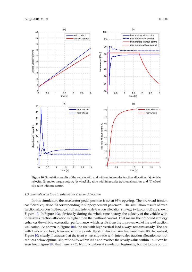
In this simulation, the accelerator pedal position is set at 95% opening. The tire/road friction coefficient equals to 0.3 corresponding to slippery cement pavement. The simulation results of even traction allocation (without control) and inter-axle traction allocation strategy (with control) are shown Figure 10. In Figure 10a, obviously during the whole time history, the velocity of the vehicle with inter-axles traction allocation is higher than that without control. That means the proposed strategy enhances the vehicle acceleration performance, which results from the improvement of the road traction utilization. As shown in Figure 10d, the tire with high vertical load always remains steady. The tire with low vertical load, however, seriously skids. Its slip ratio even reaches more than 80%. In contrast, Figure 10c clearly illustrates that the front wheel slip ratio with inter-axles traction allocation control reduces below optimal slip ratio 5.6% within 0.5 s and reaches the steady value within 2 s. It can be seen from Figure 10b that there is a 20 Nm fluctuation at simulation beginning, but the torque output stabilizes quickly after 0.5 s. At the end of the simulation, the torque reduction in Figure 10b is because the motor work point transfers from the constant torque area to constant power area.

0 0.5 1 1.5 2 2.5 30

2

4

6

8

10

12

14

16

18

20

time [s]

slip

rat

io w

ith c

ontr

ol %

(c)

0 0.5 1 1.5 2 2.5 30

10

20

30

40

50

60

70

80

90

time [s]

slip

rat

io w

ithou

t co

ntro

l %

(d)

front wheels

rear wheels front wheels

rear wheels

0 0.5 1 1.5 2 2.5 30.4

0.45

0.5

0.55

0.6

0.65

0.7

0.75

time [s]

acce

lera

tor

peda

l pos

ition

Figure 8. Simulation results of the vehicle with and without pedal self-correcting traction allocation:(a) vehicle velocity; (b) motor torque output; (c) wheel slip ratio with pedal self-correcting tractionallocation; and (d) wheel slip ratio without control.

Energies 2017, 10, 126 13 of 18

Figure 8. Simulation results of the vehicle with and without pedal self-correcting traction allocation: (a) vehicle velocity; (b) motor torque output; (c) wheel slip ratio with pedal self-correcting traction allocation; and (d) wheel slip ratio without control.

Figure 9. Accelerator pedal position under pedal self-correcting traction allocation.

4.3. Simulation on Case 3: Inter-Axles Traction Allocation

In this simulation, the accelerator pedal position is set at 95% opening. The tire/road friction coefficient equals to 0.3 corresponding to slippery cement pavement. The simulation results of even traction allocation (without control) and inter-axle traction allocation strategy (with control) are shown Figure 10. In Figure 10a, obviously during the whole time history, the velocity of the vehicle with inter-axles traction allocation is higher than that without control. That means the proposed strategy enhances the vehicle acceleration performance, which results from the improvement of the road traction utilization. As shown in Figure 10d, the tire with high vertical load always remains steady. The tire with low vertical load, however, seriously skids. Its slip ratio even reaches more than 80%. In contrast, Figure 10c clearly illustrates that the front wheel slip ratio with inter-axles traction allocation control reduces below optimal slip ratio 5.6% within 0.5 s and reaches the steady value within 2 s. It can be seen from Figure 10b that there is a 20 Nm fluctuation at simulation beginning, but the torque output stabilizes quickly after 0.5 s. At the end of the simulation, the torque reduction in Figure 10b is because the motor work point transfers from the constant torque area to constant power area.

0 0.5 1 1.5 2 2.5 30

2

4

6

8

10

12

14

16

18

20

time [s]

slip

rat

io w

ith c

ontr

ol %

(c)

0 0.5 1 1.5 2 2.5 30

10

20

30

40

50

60

70

80

90

time [s]

slip

rat

io w

ithou

t co

ntro

l %

(d)

front wheels

rear wheels front wheels

rear wheels

0 0.5 1 1.5 2 2.5 30.4

0.45

0.5

0.55

0.6

0.65

0.7

0.75

time [s]

acce

lera

tor

peda

l pos

ition

Figure 9. Accelerator pedal position under pedal self-correcting traction allocation.

Energies 2017, 10, 126 14 of 18Energies 2017, 10, 126 14 of 18

Figure 10. Simulation results of the vehicle with and without inter-axles traction allocation: (a) vehicle velocity; (b) motor torque output; (c) wheel slip ratio with inter-axles traction allocation; and (d) wheel slip ratio without control.

4.4. Simulation and Analysis on Variable Conditions

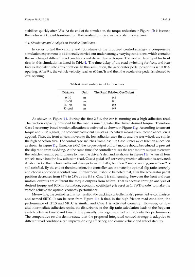
In order to test the validity and robustness of the proposed control strategy, a compressive simulation experiment is additionally carried out under strongly varying conditions, which contains the switching of different road conditions and driver desired torque. The road surface input for front tires in this simulation is listed in Table 4. The time delay of the road switching for front and rear tires is also taken into consideration. In this simulation, the accelerator pedal position is set at 85% opening. After 9 s, the vehicle velocity reaches 60 km/h and then the accelerator pedal is released to 28% opening.

Table 4. Road surface input for front tires.

Distance Unit Tire/Road Friction Coefficient0–10 m 0.8

10–50 m 0.1 50–80 m 0.2

80–end m 0.9

0 0.5 1 1.5 2 2.5 30

5

10

15

20

25

30

35

40

45

50

time [s]

vehi

cle

velo

city

[km

/h]

(a)

with control

without control

0 0.5 1 1.5 2 2.5 360

65

70

75

80

85

90

95

100

time [s]

torq

ue o

utpu

t [N

.m]

(b)

front motors with control

rear motors with controlfront motors without control

rear motors without control

0 0.5 1 1.5 2 2.5 30

2

4

6

8

10

12

14

16

18

20

time [s]

slip

rat

io w

ith c

ontr

ol %

(c)

front wheels

rear wheels

0 0.5 1 1.5 2 2.5 30

10

20

30

40

50

60

70

80

time [s]

slip

rat

io w

ithou

t co

ntro

l %(d)

front wheels

rear wheels

Figure 10. Simulation results of the vehicle with and without inter-axles traction allocation: (a) vehiclevelocity; (b) motor torque output; (c) wheel slip ratio with inter-axles traction allocation; and (d) wheelslip ratio without control.

4.3. Simulation on Case 3: Inter-Axles Traction Allocation

In this simulation, the accelerator pedal position is set at 95% opening. The tire/road frictioncoefficient equals to 0.3 corresponding to slippery cement pavement. The simulation results of eventraction allocation (without control) and inter-axle traction allocation strategy (with control) are shownFigure 10. In Figure 10a, obviously during the whole time history, the velocity of the vehicle withinter-axles traction allocation is higher than that without control. That means the proposed strategyenhances the vehicle acceleration performance, which results from the improvement of the road tractionutilization. As shown in Figure 10d, the tire with high vertical load always remains steady. The tirewith low vertical load, however, seriously skids. Its slip ratio even reaches more than 80%. In contrast,Figure 10c clearly illustrates that the front wheel slip ratio with inter-axles traction allocation controlreduces below optimal slip ratio 5.6% within 0.5 s and reaches the steady value within 2 s. It can beseen from Figure 10b that there is a 20 Nm fluctuation at simulation beginning, but the torque output

Energies 2017, 10, 126 15 of 18

stabilizes quickly after 0.5 s. At the end of the simulation, the torque reduction in Figure 10b is becausethe motor work point transfers from the constant torque area to constant power area.

4.4. Simulation and Analysis on Variable Conditions

In order to test the validity and robustness of the proposed control strategy, a compressivesimulation experiment is additionally carried out under strongly varying conditions, which containsthe switching of different road conditions and driver desired torque. The road surface input for fronttires in this simulation is listed in Table 4. The time delay of the road switching for front and reartires is also taken into consideration. In this simulation, the accelerator pedal position is set at 85%opening. After 9 s, the vehicle velocity reaches 60 km/h and then the accelerator pedal is released to28% opening.

Table 4. Road surface input for front tires.

Distance Unit Tire/Road Friction Coefficient

0–10 m 0.810–50 m 0.150–80 m 0.2

80–end m 0.9

As shown in Figure 11, during the first 2.3 s, the car is running on a high adhesion road.The traction capacity provided by the road is much greater the driver desired torque. Therefore,Case 1 economy-based traction allocation is activated as shown in Figure 11g. According to currenttorque and RPM signals, the economy coefficient p is set as 0.5, which means even traction allocation isapplied. Then, the front wheels move into the low adhesion area firstly and the rear wheels are still inthe high adhesion area. The control case switches from Case 1 to Case 3 inter-axles traction allocationas shown in Figure 11g. Based on SMC, the torque output of front motors should be reduced to preventthe slip ratio from skidding. At the same time, the controller raises the rear motors output to ensurethe vehicle dynamic performance to meet the driver’s demand as shown in Figure 11c. When all fourwheels move into the low adhesion road, Case 2 pedal self-correcting traction allocation is activated.At about 6.4 s, the friction coefficient changes from 0.1 to 0.2, but Case 2 keeps running, since Case 2 isstill satisfied. By the end of the simulation, the controller can estimate the optimal slip ratio correctlyand choose appropriate control case. Furthermore, it should be noted that, after the accelerator pedalposition decreases from 85% to 28% at the 8.9 s, Case 1 is still running, however the front and rearmotors’ outputs are different the torque outputs from before. That is because through analysis ofdesired torque and RPM information, economy coefficient p is reset as 1, FWD mode, to make thevehicle achieve the optimal economy performance.

Meanwhile, the control results from a slip ratio tracking controller is also presented as comparisonand named SRTC. It can be seen from Figure 11e–h that, in the high friction road condition, theperformance of ITCS and SRTC is similar and Case 1 is activated correctly. However, on lowand intermediate adhesion roads, the disturbance of the slip ratio calculation leads to the frequentswitch between Case 2 and Case 3. It apparently has negative effect on the controller performance.The comparative results demonstrate that the proposed integrated control strategy is adaptive todifferent road conditions, can improve driving efficiency, and ensure vehicle and wheel stability.

Energies 2017, 10, 126 16 of 18

Energies 2017, 10, 126 15 of 18

As shown in Figure 11, during the first 2.3 s, the car is running on a high adhesion road. The traction capacity provided by the road is much greater the driver desired torque. Therefore, Case 1 economy-based traction allocation is activated as shown in Figure 11g. According to current torque and RPM signals, the economy coefficient p is set as 0.5, which means even traction allocation is applied. Then, the front wheels move into the low adhesion area firstly and the rear wheels are still in the high adhesion area. The control case switches from Case 1 to Case 3 inter-axles traction allocation as shown in Figure 11g. Based on SMC, the torque output of front motors should be reduced to prevent the slip ratio from skidding. At the same time, the controller raises the rear motors output to ensure the vehicle dynamic performance to meet the driver’s demand as shown in Figure 11c. When all four wheels move into the low adhesion road, Case 2 pedal self-correcting traction allocation is activated. At about 6.4 s, the friction coefficient changes from 0.1 to 0.2, but Case 2 keeps running, since Case 2 is still satisfied. By the end of the simulation, the controller can estimate the optimal slip ratio correctly and choose appropriate control case. Furthermore, it should be noted that, after the accelerator pedal position decreases from 85% to 28% at the 8.9 s, Case 1 is still running, however the front and rear motors’ outputs are different the torque outputs from before. That is because through analysis of desired torque and RPM information, economy coefficient p is reset as 1, FWD mode, to make the vehicle achieve the optimal economy performance.

Meanwhile, the control results from a slip ratio tracking controller is also presented as comparison and named SRTC. It can be seen from Figure 11e–h that, in the high friction road condition, the performance of ITCS and SRTC is similar and Case 1 is activated correctly. However, on low and intermediate adhesion roads, the disturbance of the slip ratio calculation leads to the frequent switch between Case 2 and Case 3. It apparently has negative effect on the controller performance. The comparative results demonstrate that the proposed integrated control strategy is adaptive to different road conditions, can improve driving efficiency, and ensure vehicle and wheel stability.

0 2 4 6 8 100

20

40

60

80

100

120

time [s]

disp

lace

men

t [m

]

(a)

0 2 4 6 8 100

10

20

30

time [s]

optim

al s

lip r

atio

%

(b)

front wheels

rear wheels

0 2 4 6 8 10

0

50

100

150

time [s]

mot

or t

orqu

e [N

.m]

(c)

front mototrs

rear mototrs

0 2 4 6 8 100

20

40

60

80

time [s]

vehi

cle

velo

city

[km

/h]

(d)

Energies 2017, 10, 126 16 of 18

Figure 11. Simulation results on variable conditions: (a) longitudinal displacement of front wheels; (b) optimal slip ratio estimation; (c) motor torque output; (d) vehicle longitudinal velocity; (e) wheel slip ratio of ITCS; (f) wheel slip ratio of SRTC; (g) control case switch of ITCS; and (h) control case switch of SRTC.

5. Conclusions

In this paper, a novel ITCS for DDEVs is proposed, aiming at improving economy, vehicle stability and dynamic performance. Firstly, for the issue that the motor efficiency varies greatly in different working conditions, economy-based traction allocation strategy is developed. According to the economy coefficient, driver desired torque is distributed reasonably among four driving motors, which maximizes the motor driving efficiency and improves overall vehicle economy. Simulation results reveal that compared with 4WETD and FWD, the economy-based traction allocation can decrease energy consumption 3.584% and 1.992%, respectively, according to the New European driving cycle. Meanwhile, pedal self-correcting traction allocation and inter-axles traction allocation is designed to overcome vehicle stability problems on low adhesion road. By means of Bayes theorem, optimal slip ratio on different road surfaces can be obtained in real time. Based on SMC, the torque output of each motor is adjusted to keep the wheel rotational speed under the reference value rapidly and stably. It is also verified that the tire skid phenomenon can be suppressed within 0.5 s. On basis of the methods mentioned above, the integrated control strategy is finally presented. It can balance the relationship between road/tire friction conditions, motor efficiency and driver desired torque; and achieve vehicle economy and longitudinal stability optimization.

Further research may concentrate in the following aspects:

(1) When vehicle lateral motion is taken into account, the ITCS needs a good combination of the other stability control systems, such as electronic stability control (ESC).

(2) Since the proposed method is only analyzed theoretically and validated via simulation, an actual bench or field test is needed in the future to verify the proposed control strategy.

Acknowledgments: The work was supported by the Berlin City Vehicle (BCV) Project in Technical University of Berlin (TU-Berlin). The authors would like to thank China Scholarship Council (CSC) for providing a scholarship as the financial support for the first author to pursue his Ph.D. degree at TU Berlin. Finally, the authors also acknowledge support by the German Research Foundation and the Open Access Publication Funds of Technische Universität Berlin.

0 2 4 6 8 10

0

2

4

6

8

time [s]

slip

rat

io o

f IT

CS

%

(e)

front wheels

rear wheels

0 2 4 6 8 10

0

2

4

6

8

time [s]

slip

rat

io o

f S

RT

C %

(f)

front wheels

rear wheels

0 2 4 6 8 101

1.5

2

2.5

3

time [s]

cont

rol c

ase

switc

h of

IT

CS

(g)

0 2 4 6 8 101

1.5

2

2.5

3

time [s]

cont

rol c

ase

switc

h of

SR

TC

(h)

Figure 11. Simulation results on variable conditions: (a) longitudinal displacement of front wheels;(b) optimal slip ratio estimation; (c) motor torque output; (d) vehicle longitudinal velocity; (e) wheelslip ratio of ITCS; (f) wheel slip ratio of SRTC; (g) control case switch of ITCS; and (h) control caseswitch of SRTC.

5. Conclusions

In this paper, a novel ITCS for DDEVs is proposed, aiming at improving economy, vehicle stabilityand dynamic performance. Firstly, for the issue that the motor efficiency varies greatly in differentworking conditions, economy-based traction allocation strategy is developed. According to theeconomy coefficient, driver desired torque is distributed reasonably among four driving motors, whichmaximizes the motor driving efficiency and improves overall vehicle economy. Simulation results

Energies 2017, 10, 126 17 of 18

reveal that compared with 4WETD and FWD, the economy-based traction allocation can decreaseenergy consumption 3.584% and 1.992%, respectively, according to the New European driving cycle.Meanwhile, pedal self-correcting traction allocation and inter-axles traction allocation is designed toovercome vehicle stability problems on low adhesion road. By means of Bayes theorem, optimal slipratio on different road surfaces can be obtained in real time. Based on SMC, the torque output of eachmotor is adjusted to keep the wheel rotational speed under the reference value rapidly and stably. It isalso verified that the tire skid phenomenon can be suppressed within 0.5 s. On basis of the methodsmentioned above, the integrated control strategy is finally presented. It can balance the relationshipbetween road/tire friction conditions, motor efficiency and driver desired torque; and achieve vehicleeconomy and longitudinal stability optimization.

Further research may concentrate in the following aspects:

(1) When vehicle lateral motion is taken into account, the ITCS needs a good combination of theother stability control systems, such as electronic stability control (ESC).

(2) Since the proposed method is only analyzed theoretically and validated via simulation, an actualbench or field test is needed in the future to verify the proposed control strategy.

Acknowledgments: The work was supported by the Berlin City Vehicle (BCV) Project in Technical University ofBerlin (TU-Berlin). The authors would like to thank China Scholarship Council (CSC) for providing a scholarshipas the financial support for the first author to pursue his Ph.D. degree at TU Berlin. Finally, the authors alsoacknowledge support by the German Research Foundation and the Open Access Publication Funds of TechnischeUniversität Berlin.

Author Contributions: Xudong Zhang and Dietmar Göhlich proposed the control strategy; Xudong Zhangprogramed and debugged the simulation experiments; Dietmar Göhlich contributed the simulation tools;all authors carried out data analysis, discussed results and contributed to write the paper.

Conflicts of Interest: The authors declare that there is no conflict of interests regarding the publication ofthis paper.

References

1. Hori, Y.; Toyoda, Y.; Tsuruoka, Y. Traction control of electric vehicle: Basic experimental results using the testEV “UOT Electric March”. IEEE Trans. Ind. Appl. 1998, 34, 1131–1138. [CrossRef]

2. Esmailzadeh, E.; Vossoughi, G.R.; Goodarzi, A. Dynamic modelling and analysis of a four motorized wheelselectric vehicle. Int. J. Veh. Syst. Dyn. 2001, 35, 163–194. [CrossRef]

3. Fujii, K.; Fujimoto, H. Traction control based on slip ratio estimation without detecting vehicle speed forelectric vehicle. In Proceedings of the Fourth Power Conversion Conference-Nagoya 2007, Nagoya, Japan,2–5 April 2007; pp. 688–693.

4. Hori, Y. Future vehicle driven by electricity and control-research on four-wheel-motored “UOT ElectricMarch II”. IEEE Trans. Ind. Electron. 2004, 51, 954–962. [CrossRef]

5. Khatun, P.; Bingham, C.M.; Mellor, P.H. Comparison of Control Methods for Electric Vehicle Antilock Braking/TractionControl Systems; SAE Technical Paper No. 2001-01-0596; SAE International: Warrendale, PA, USA, 2001.

6. Ratiroch-Anant, P.; Hirata, H.; Anabuki, M.; Ouchi, S. Adaptive controller design for anti-slip system ofEV. In Proceedings of the IEEE Conference on Robotics, Automation and Mechatronics, Bangkok, Thailand,1–3 June 2006; pp. 1–6.

7. Deur, J.; Pavkovic, D.; Burgio, G.; Hrovat, D. A model-based traction control strategy non-reliant on wheelslip information. Int. J. Veh. Syst. Dyn. 2011, 49, 1245–1265. [CrossRef]

8. Bottiglione, F.; Sorniotti, A.; Shead, L. The effect of half-shaft torsion dynamics on the performance of a tractioncontrol system for electric vehicles. Proc. Inst. Mech. Eng. Part D J. Automob. Eng. 2012, 226, 1145–1159. [CrossRef]

9. Leiber, H.; Czinczel, A. Four Years of Experience with 4-Wheel Antiskid Brake Systems (ABS); SAE TechnicalPaper No. 830481; SAE International: Warrendale, PA, USA, 1983.

10. Zhao, Z. Research on Vehicle Dynamics, Its Nonlinear Control Strategies and Related Technologies.Ph.D. Thesis, Northwestern Polytechnical University, Xi’an, China, 2002.

11. Khatun, P.; Bingham, C.M.; Schofield, N.; Mellor, P.H. Application of fuzzy control algorithms for electricvehicle antilock braking/traction control systems. IEEE Trans. Veh. Technol. 2003, 52, 1356–1364. [CrossRef]

Energies 2017, 10, 126 18 of 18

12. Yin, D.; Oh, S.; Hori, Y. A novel traction control for EV based on maximum transmissible torque estimation.IEEE Trans. Ind. Electron. 2009, 56, 2086–2094.

13. Sakai, S.I.; Sado, H.; Hori, Y. Anti-skid control with motor in electric vehicle. In Proceedings of the 6thInternational Workshop on Advanced Motion Control, Nagoya, Japan, 30 March–1 April 2000; pp. 317–322.

14. Amodeo, M.; Ferrara, A.; Terzaghi, R.; Vecchio, C. Wheel slip control via second-order sliding-modegeneration. IEEE Trans. Intell. Transp. Syst. 2010, 11, 122–131. [CrossRef]

15. Cho, K.; Kim, J.; Choi, S. The integrated vehicle longitudinal control system for ABS and TCS. In Proceedingsof the IEEE International Conference on Control Applications (CCA), Dubrovnik, Croatia, 3–5 October 2012.

16. Tanelli, M.; Ferrara, A. Wheel slip control of road vehicles via switched second order sliding modes. Int. J.Veh. Des. 2013, 62, 231–253. [CrossRef]

17. Drakunov, S.; Özgüner, U.; Dix, P.; Ashrafi, B. ABS control using optimum search via sliding modes.IEEE Trans. Control Syst. Technol. 1995, 3, 79–85. [CrossRef]

18. Unsal, C.; Kachroo, P. Sliding mode measurement feedback control for antilock braking systems. IEEE Trans.Control Syst. Technol. 1999, 7, 271–281. [CrossRef]

19. He, H.; Peng, J.; Xiong, R.; Fan, H. An acceleration slip regulation strategy for four-wheel drive electricvehicles based on sliding mode control. Energies 2014, 7, 3748–3763. [CrossRef]

20. Nam, K.; Hori, Y.; Lee, C. Wheel Slip Control for Improving Traction-Ability and Energy Efficiency ofa Personal Electric Vehicle. Energies 2015, 8, 6820–6840. [CrossRef]

21. Yuan, X.; Wang, J. Torque distribution strategy for a front-and rear-wheel-driven electric vehicle. IEEE Trans.Veh. Technol. 2012, 61, 3365–3374. [CrossRef]

22. Mokhiamar, O.; Abe, M. Active wheel steering and yaw moment control combination to maximize stabilityas well as vehicle responsiveness during quick lane change for active vehicle handling safety. Proc. Inst.Mech. Eng. Part D J. Automob. Eng. 2002, 216, 115–124. [CrossRef]

23. Mokhiamar, O.; Abe, M. How the four wheels should share forces in an optimum cooperative chassis control.Control Eng. Pract. 2006, 14, 295–304. [CrossRef]

24. He, P.; Hori, Y. Improvement of EV maneuverability and safety by disturbance observer based dynamicforce distribution. In Proceedings of the EVS22 International Electric Vehicle Symposium and Exhibition,Yokohama, Japan, 23–28 October 2006.

25. Nishihara, O.; Kumamoto, H. Minimax optimizations of tire workload exploiting complementarities betweenindependent steering and traction/braking force distributions. In Proceedings of the AVEC ’06, InternationalSymposium on Advanced Vehicle Control, Taipei, Taiwan, 20–24 August 2006; pp. 713–718.

26. Yamakawa, J.; Watanabe, K. A method of optimal wheel torque determination for independent wheel drivevehicles. J. Terramechanics 2006, 43, 269–285. [CrossRef]

27. Zareian, A.; Azadi, S.; Kazemi, R. Estimation of road friction coefficient using extended Kalman filter, recursiveleast square, and neural network. Proc. Inst. Mech. Eng. Part K J. Multi-Body Dyn. 2016, 230, 52–68. [CrossRef]

28. Guan, H.; Wang, B.; Lu, P.; Xu, L. Identification of maximum road friction coefficient and optimal slip ratiobased on road type recognition. Chin. J. Mech. Eng. 2014, 27, 1018–1026. [CrossRef]

29. Zimmermann, M. Loss Calculation of an Electric Drive Train Using a Standard Driving Cycle. Master’s Thesis,Technical University of Berlin, Berlin, Germany, 2013.

30. Zhang, X.; Göhlich, D.; Wu, X.L. Optimal torque distribution strategy for a four motorized wheels electricvehicle. In Proceedings of the EVS28 International Electric Vehicle Symposium and Exhibition, Goyang,Korea, 3–6 May 2015.

31. Ray, L.R. Real time determination of road coefficient of friction for IVHS and advanced vehicle control.In Proceedings of the American Control Conference, Seattle, WA, USA, 21–23 June 1995; Volume 3,pp. 2133–2137.

32. Wenzel, T.A.; Burnham, K.J.; Blundell, M.V.; Williams, R.A. Dual extended Kalman filter for vehicle state andparameter estimation. Int. J. Veh. Syst. Dyn. 2006, 44, 153–171. [CrossRef]

© 2017 by the authors; licensee MDPI, Basel, Switzerland. This article is an open accessarticle distributed under the terms and conditions of the Creative Commons Attribution(CC BY) license (http://creativecommons.org/licenses/by/4.0/).