Integrated Surface-groundwater Flow Modeling: a Free ...
40
UCRL-JRNL-211468 Integrated Surface-groundwater Flow Modeling: a Free-surface Overland Flow Boundary Condition in a Parallel Groundwater Flow Model S. J. Kollet, R. M. Maxwell April 18, 2005 Advances in Water Resources
Transcript of Integrated Surface-groundwater Flow Modeling: a Free ...
UCRL-JRNL-211468
Integrated Surface-groundwater FlowModeling: a Free-surface Overland FlowBoundary Condition in a ParallelGroundwater Flow Model
S. J. Kollet, R. M. Maxwell
April 18, 2005
Advances in Water Resources

Disclaimer
This document was prepared as an account of work sponsored by an agency of the United States Government. Neither the United States Government nor the University of California nor any of their employees, makes any warranty, express or implied, or assumes any legal liability or responsibility for the accuracy, completeness, or usefulness of any information, apparatus, product, or process disclosed, or represents that its use would not infringe privately owned rights. Reference herein to any specific commercial product, process, or service by trade name, trademark, manufacturer, or otherwise, does not necessarily constitute or imply its endorsement, recommendation, or favoring by the United States Government or the University of California. The views and opinions of authors expressed herein do not necessarily state or reflect those of the United States Government or the University of California, and shall not be used for advertising or product endorsement purposes.
Integrated surface-groundwater flow modeling: a free-surface overland flow boundary condition in a parallel groundwater flow model
Stefan J. Kollet and Reed M. Maxwell Environmental Science Division, Lawrence Livermore National Laboratory (L-208), 7000 East Avenue, Livermore, CA 94550 USA, E-mail: [email protected], Phone: 925-422-9297, Fax: 925-422-3118
Abstract
Interactions between surface and ground water are a key component of the hydrologic budget on the
watershed scale. Models that honor these interactions are commonly based on the conductance concept
that presumes a distinct interface at the land surface, separating the surface from the subsurface
domain. These types of models link the subsurface and surface domains via an exchange flux that
depends upon the magnitude and direction of the hydraulic gradient across the interface and a
proportionality constant (a measure of the hydraulic connectivity). Because experimental evidence of
such a distinct interface is often lacking in field systems, there is a need for a more general coupled
modeling approach.
A more general coupled model is presented that incorporates a new two-dimensional overland flow
simulator into the parallel three-dimensional variable saturated subsurface flow code ParFlow. In
ParFlow, the overland flow simulator takes the form of an upper boundary condition and is, thus, fully
integrated without relying on the conductance concept. Another important advantage of this approach is
the efficient parallelism incorporated into ParFlow, which is efficiently exploited by the overland flow
simulator.
Several verification and simulation examples are presented that focus on the two main processes of
runoff production : excess infiltration and saturation. The model is shown to reproduce an analytical
solution for overland flow and compares favorably to other commonly used hydrologic models. The
influence of heterogeneity of the shallow subsurface on overland flow is also examined. The results
show the uncertainty in overland flow predictions due to subsurface heterogeneity and demonstrate the
usefulness of our approach. Both the overland flow component and the coupled model are evaluated in
a parallel scaling study and show to be efficient.
1 Introduction
The subsurface and surface are complex environmental systems that often behave in a coupled manner.
Surface water in rivers, streams, lakes and wetlands is in constant communication with the vadose
zone, shallow and deep groundwater systems. Thus, surface-groundwater interactions are an intrinsic
component of the hydrologic budget on the watershed scale and hydrologic modeling tools must
account for this interaction to provide reliable predictions. Surface-groundwater interacions have been
a widely recognized research area by several scientific communities interested in different spatial
scales varying from bedform scale in hyporheic exchange modeling to continental scale hydrologic
response modeling.
The occurrence of surface water and its spatial and temporal distribution depends on climatic factors
(e.g., amount and distribution of rainfall and temperature), vegetation, topography (micro and macro),
and on the exchange of water between the surface and the sub-surface. The rate and direction of
exchange (groundwater discharge at the land surface or surface water infiltration into the subsurface)
depend on the rainfall rate, direction of the hydraulic gradient and hydraulic characteristics of the land
surface.
The two major processes of runoff production are commonly referred to as Hortonian and Dunne
runoff. Hortonian runoff, often referred to as excess infiltration, occurs when the rainfall rate exceeds
the saturated hydraulic conductivity of the land surface. Under excess infiltration conditions, ponding
(accumulation of water at the surface) can occur before the subsurface becomes entirely saturated
(Kutilek and Nielsen, 1994). Dunne runoff, often referred to as excess saturation, occurs when the
rainfall rate is smaller or equal to the saturated hydraulic conductivity of the land surface. Under excess
saturation conditions, ponding can occur only when the entire soil column becomes completely
saturated and water exfiltrates at the surface (Kutilek and Nielsen, 1994). Although these two processes
are often considered independent, in the presence of a non-uniform distribution of soil properties,
infiltration and saturation excess are interrelated and may occur simultaneously at various spatial and
temporal scales.
Traditionally, the coupling of the surface and subsurface domains has been done via a so-called
exchange flux that appears in both the groundwater and surface water flow equations as general
sink/source terms. In this approach, the exchange rate is expressed in terms of the conductance concept
which assumes an interface connecting the two domains (e.g., Anderson and Woessner 1992;
VanderKwaak and Loague, 2001). This interface is commonly characterized by a proportionality
constant representing the connectivity between the surface and sub-surface and generally involves the
ratio of the interface hydraulic conductivity and effective thickness (e.g., Hantush, 1965). Recent
studies have included additional processes into the conductance concept to account for the influence of
microtopography on surface saturation (VanderKwaak and Loague, 2001; Panday and Huyakorn,
2004). In many cases, the application of the conductance concept to real systems is problematic,
because the existence of a distinct interface has yet to be demonstrated in the field (Kollet and Zlotnik,
2003; Cardenas and Zlotnik, 2003 ).
Numerical algorithms for solving the problem of variable saturated groundwater flow are widely
available and have been published extensively (e.g., Huyakorn et al., 1986; Kirkland et al., 1992;
Forsyth et al., 1995; Therrien and Sudicky, 1996; Miller et al., 1998; Jones and Woodward, 2001).
Overland flow simulators have been also studied extensively, though major problems with
inappropriate stability criteria remain to be a problem in many cases (Taylor et al., 1974; Gottardi and
Ventulli, 1993; Fiedler and Ramirez, 2000; Jaber and Mohtar, 2003). The coupling of surface and sub-
surface flow also received considerable attention recently, with most models coupled in a linked
fashion, iterating over the exchange flux until some convergence criterion is reached. This approach
may cause large mass balance errors (e.g., LaBolle et al., 2003) and numerical instabilities, because of
the large differences in the time scales of the two processes (surface runoff occurring on a much shorter
time scale than the subsurface). Previous studies are summarized briefly below.
Freeze and Harlan (1969) provided the first comprehensive conceptual and theoretical framework of an
integrated hydrologic response model on the watershed scale. Later, Govindaraju and Kavvas (1991)
developed a coupled model that accounts for 1D channel and overland flow and 3D variable saturated
groundwater flow. They studied the response of variable source areas (saturated areas adjacent to the
stream) to hydrologic and topographic variations. Woolhiser at al. (1996) studied the effect of
subsurface heterogeneity in the hydraulic conductivity using an overland flow model coupled to the
Smith-Parlange infiltration model. They demonstrated the effect of heterogeneity on the hydrograph
and presented a technique that accounted for the influence of microtopography. Wallach et al. (1997)
studied the error in the exchange rate between the surface and the subsurface when the exchange rate is
calculated assuming zero ponding depth. Fiedler and Ramirez (2000) solved the 2D hydrodynamic flow
equations using MacCormack finite differences. In their model, interactive infiltration is simulated
using the Green-Ampt formulation. Gunduz and Aral (2004) solve the problem of coupled groundwater
and 1D channel flow by forming a single matrix instead of solving two separate matrices for the two
domains. Braunschweig et al. (2004) presented an integrated hydrologic modeling system that
incorporates routing of water inside channels and on the land surface coupled to infiltration processes.
Putti and Paniconi (2004) discussed numerical issues, such as the influence of the time step size on the
global convergence behavior, in coupling a 3D variable saturated flow model with a 1D diffusion
formulation of the overland flow equations. VanderKwaak and Loague (2001) and Panday and
Huyakorn (2004) presented fully coupled approaches including land surface processes, such as
evaporation, and demonstrated their usefulness. A common theme among previous work summarized
here is that these models rely on some form of the conductance concept. The current work presented in
this paper differs from these studies in that it provides a framework for a more general approach.
This study presents a general framework for coupling the surface and groundwater flow equations,
which does not rely on the conductance concept. The surface water equations are used to close the
initial value problem of variable saturated groundwater flow, which results in an overland flow
boundary condition. This overland flow boundary condition, which has not been published before in
the presented form to our knowledge, takes into account the free surface of water ponded at the land
surface. To demonstrate the usefulness of this approach, we developed a two-dimensional distributed
overland flow simulator, which was implemented into the three-dimensional, variable saturated
groundwater flow code ParFlow . We present verification and simulation examples that focus on the
surface water component independently and the aforementioned processes of excess infiltration and
saturation. We introduce subsurface heterogeneity in the hydraulic conductivity tensor resulting in
surface runoff and hydrograph uncertainty. ParFlow was designed for parallel computer systems and
has been used extensively in large-scale and high resolution modeling (Ashby and Falgout, 1996; Jones
and Woodward, 2001). The overland flow simulator exploits ParFlow’s parallel infrastructure
effectively and is also fully parallel, which is demonstrated in a parallel efficiency study.
2 Theory
As mentioned in the Section 1, the theory of coupled surface-water groundwater systems has been the
subject of many previous studies. Hence, the governing equations of overland flow and variable
saturated groundwater flow have been discussed in great detail in the literature. We therefore, provide
only a brief summary of these equations that form the basis for the set of coupled equations presented
later in Section 2.5.
2.1 Shallow Overland Flow
In two spatial dimensions, the continuity equation can be written as
( )xqxqvt ers
s −−∇=∂
∂ )(ψψ v (1)
where vv is the depth averaged velocity vector [LT-1]; ψs is the surface ponding depth [L], qr(x) is the
rainfall rate [LT-1] and qe(x) is the exchange rate with the subsurface [L], which will be discussed in
detail below. Note, that in Equation (1) the flow depth is vertically averaged. Thus, vertical change of
momentum in the column of ponded water is neglected in this formulation. This has been shown to be a
good approximation for shallow systems.
If diffusion terms are neglected the momentum equation can be written as
Sf,i = So,i (2)
which is commonly referred to as the kinematic wave approximation. In Eq 2 So,i is the bed slope
(gravity forcing term) [-], which is equal to the friction slope Sf,i [L]; i stands for the x- and y-direction.
Although we consider the kinematic wave in the current work, this formulation can be expanded to
incorporate the diffusive and dynamic wave equations (Fiedler and Ramirez, 2000) .
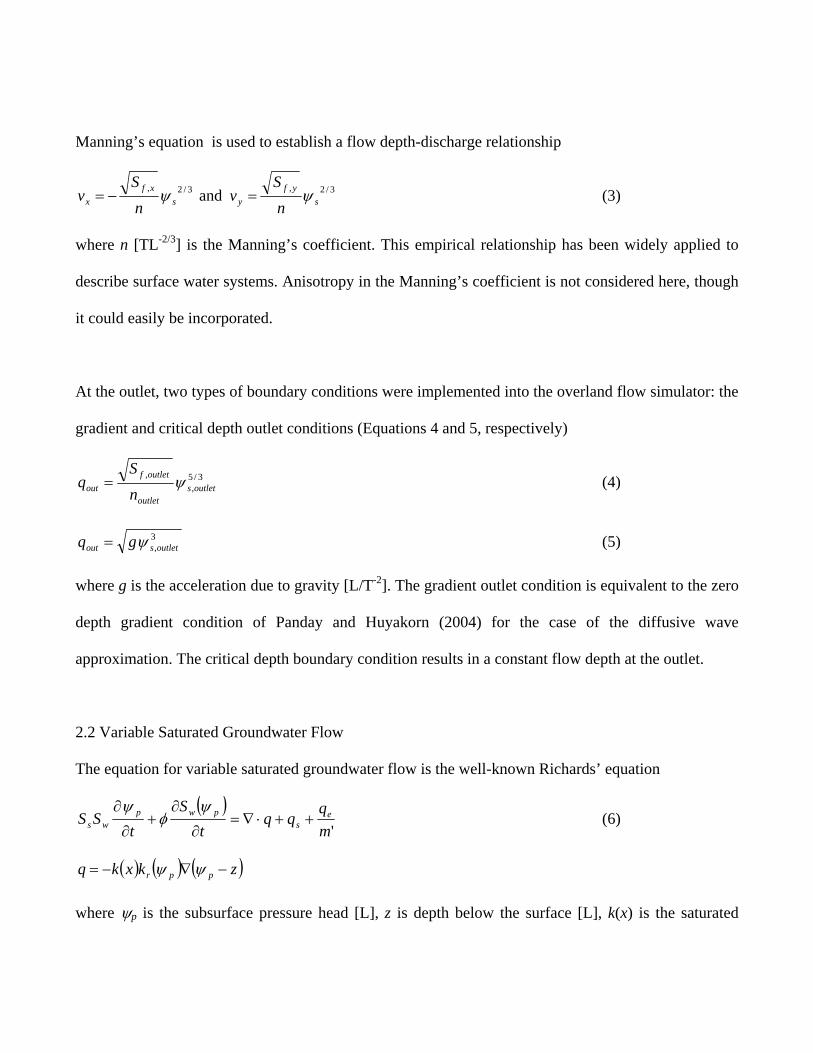
Manning’s equation is used to establish a flow depth-discharge relationship
3/2,s
xfx n
Sv ψ−= and 3/2,
syf
y nS
v ψ= (3)
where n [TL-2/3] is the Manning’s coefficient. This empirical relationship has been widely applied to
describe surface water systems. Anisotropy in the Manning’s coefficient is not considered here, though
it could easily be incorporated.
At the outlet, two types of boundary conditions were implemented into the overland flow simulator: the
gradient and critical depth outlet conditions (Equations 4 and 5, respectively)
3/5,
,outlets
outlet
outletfout n
Sq ψ= (4)
3,outletsout gq ψ= (5)
where g is the acceleration due to gravity [L/T-2]. The gradient outlet condition is equivalent to the zero
depth gradient condition of Panday and Huyakorn (2004) for the case of the diffusive wave
approximation. The critical depth boundary condition results in a constant flow depth at the outlet.
2.2 Variable Saturated Groundwater Flow
The equation for variable saturated groundwater flow is the well-known Richards’ equation
( )'m
qqq
tS
tSS e
spwp
ws ++⋅∇=∂
∂+
∂
∂ ψφ
ψ (6)
( ) ( ) ( )zkxkq ppr −∇−= ψψ
where ψp is the subsurface pressure head [L], z is depth below the surface [L], k(x) is the saturated
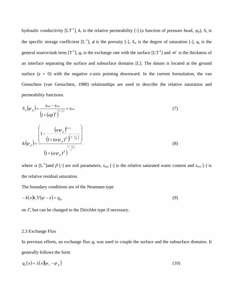
hydraulic conductivity [LT-1], kr is the relative permeability [-] (a function of pressure head, ψp), Ss is
the specific storage coefficient [L-1], φ is the porosity [-], Sw is the degree of saturation [-], qs is the
general source/sink term [T-1], qe is the exchange rate with the surface [LT-1] and is the thickness of
an interface separating the surface and subsurface domains [L]. The datum is located at the ground
surface (z = 0) with the negative z-axis pointing downward. In the current formulation, the van
Genuchten (van Genuchten, 1980) relationships are used to describe the relative saturation and
permeability functions.
m′
( )( )( )
( ) resn
ressatpw s
p
ssSn
++
−=
− 11
1 αψ (7)
( )
( )( )
( ) 2
11
)(1
)(11
11
1
⎟⎠⎞⎜
⎝⎛ −
+
⎟⎟⎟
⎠
⎞
⎜⎜⎜
⎝
⎛
+−
=⎟⎠⎞⎜
⎝⎛ −
−
β
β
ββ
β
αψ
αψ
αψ
ψ
p
p
p
prk (8)
where α [L-1]and β [-] are soil parameters, ssat [-] is the relative saturated water content and sres [-] is
the relative residual saturation.
The boundary conditions are of the Neumann type
( ) ( ) bcr qzkxk =−∇− ψ (9)
on Γ, but can be changed to the Dirichlet type if necessary.
2.3 Exchange Flux
In previous efforts, an exchange flux qe was used to couple the surface and the subsurface domains. It
generally follows the form
( ) ( )( )pse xxq ψψλ −= (10)
Thus, the exchange rate depends upon the gradient across some interface and the proportionality
constant λ(x) [T-1], which is a measure of the hydraulic connectivity between the two domains (Figure
1). This concept has been used extensively in studies concerned with the interactions of surface-
subsurface flow and is also known as the conductance concept with λ being the conductance coefficient
(Hantush, 1965; Anderson and Woessner, 1992 ).
Often the system of equations outlined above is solved iteratively. For example, one might iterate over
qe until some convergence criteria is fulfilled. However, since overland flow time scales may be much
smaller than groundwater flow time scales, numerical instabilities often arise, necessitating adaptive
time stepping and/or a fully integrated approach to solve the system of equations simultaneously (e.g.,
Panday and Huyakorn, 2004).
A perhaps even greater limitation of this approach lies in the assumption that there exists some distinct
interface between the surface and subsurface and in the ensuing definition of the proportionality
constant λ. For example, λ generally depends upon the ratio of some interface permeability k ′ and the
interface thickness . It is difficult to establish evidence of such a distinct interface from direct field
observations (Cardenas and Zlotnik, 2003; Kollet and Zlotnik, 2003). Additionally, often a simplifying
assumption of spatial uniformity in the hydraulic interface properties is applied, because of a lack of
field data. In many cases, no in-situ measurements are available and λ is used solely as a fitting
parameter. The question arises, whether the conductance concept is actually a useful conceptual model
of interactions between the surface and the subsurface, and implies the necessity of a more general
formulation.
m′
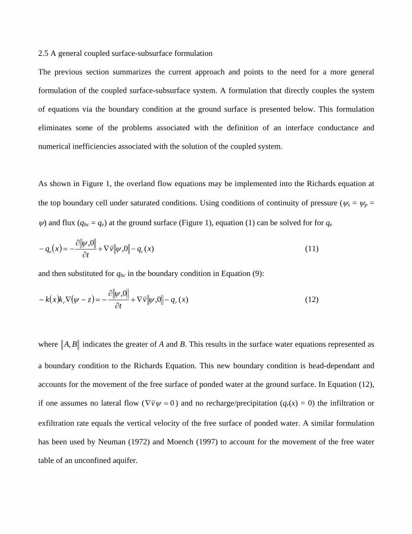
2.5 A general coupled surface-subsurface formulation
The previous section summarizes the current approach and points to the need for a more general
formulation of the coupled surface-subsurface system. A formulation that directly couples the system
of equations via the boundary condition at the ground surface is presented below. This formulation
eliminates some of the problems associated with the definition of an interface conductance and
numerical inefficiencies associated with the solution of the coupled system.
As shown in Figure 1, the overland flow equations may be implemented into the Richards equation at
the top boundary cell under saturated conditions. Using conditions of continuity of pressure (ψs = ψp =
ψ) and flux (qbc = qe) at the ground surface (Figure 1), equation (1) can be solved for for qe
( ) )(0,0,
xqvt
xq re −∇+∂
∂−=− ψ
ψ v (11)
and then substituted for qbc in the boundary condition in Equation (9):
( ) ( ) )(0,0,
xqvt
zkxk rr −∇+∂
∂−=−∇− ψ
ψψ v (12)
where BA, indicates the greater of A and B. This results in the surface water equations represented as
a boundary condition to the Richards Equation. This new boundary condition is head-dependant and
accounts for the movement of the free surface of ponded water at the ground surface. In Equation (12),
if one assumes no lateral flow ( 0=∇ ψvv ) and no recharge/precipitation (qr(x) = 0) the infiltration or
exfiltration rate equals the vertical velocity of the free surface of ponded water. A similar formulation
has been used by Neuman (1972) and Moench (1997) to account for the movement of the free water
table of an unconfined aquifer.
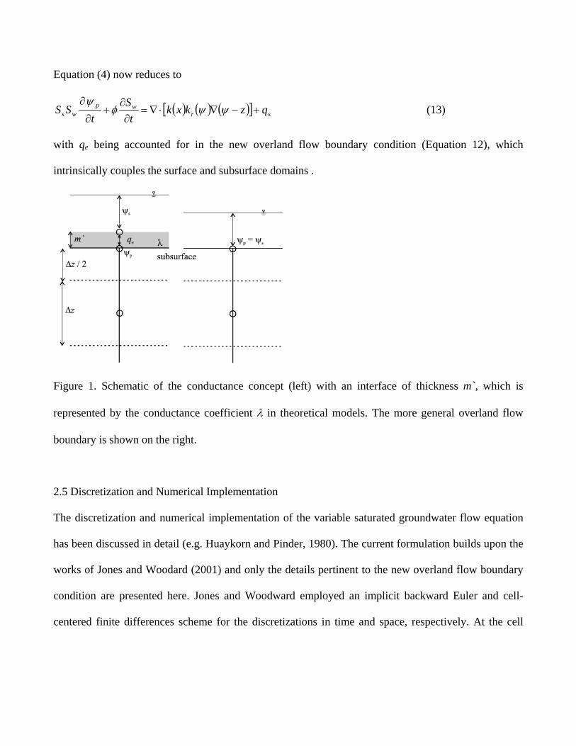
Equation (4) now reduces to
( ) ( ) ( )[ srwp
ws qzkxkt
St
SS +−∇⋅∇=∂
∂+
∂
∂ψψφ ]ψ
(13)
with qe being accounted for in the new overland flow boundary condition (Equation 12), which
intrinsically couples the surface and subsurface domains .
Figure 1. Schematic of the conductance concept (left) with an interface of thickness m`, which is
represented by the conductance coefficient λ in theoretical models. The more general overland flow
boundary is shown on the right.
2.5 Discretization and Numerical Implementation
The discretization and numerical implementation of the variable saturated groundwater flow equation
has been discussed in detail (e.g. Huaykorn and Pinder, 1980). The current formulation builds upon the
works of Jones and Woodard (2001) and only the details pertinent to the new overland flow boundary
condition are presented here. Jones and Woodward employed an implicit backward Euler and cell-
centered finite differences scheme for the discretizations in time and space, respectively. At the cell
interfaces, the harmonic averages of the saturated hydraulic conductivities and a one-point upstream
weighting of the relative permeabilities are used.
For the overland flow component, a standard upwind finite control volume scheme was used for the
spatial discretization and an implicit backward Euler scheme in time. The advantage of the spatial
discretization methods applied in this study is that they are locally mass conservative. Discretization
errors for Richards equation have been analyzed extensively by Woodward and Dawson (2000).
The solver implemented in the current study is described by Jones and Woodard (2001) and is a
Newton-Krylov solution method (e.g., Saad, 2003). Newton-Krylov methods are based on a Newton
linearization of the nonlinear system. The Jacobian is then solved with an iterative Krylov method. An
advantage of this method is that the Krylov solver only requires matrix-vector products not the solution
of the matrix itself. Additionally, Jones and Woodward (2001) preconditioned the linear system with an
approximated Jacobian to improve convergence. In this study, the diagonal of the preconditioner matrix
was modified to account for the overland flow boundary condition. As shown in below, this proved to
be an efficient approximation of the Jacobian.
3 Numerical Simulations, Results and Discussion
No analytical solution exists for the coupled surface-subsurface system of equations presented in
Section 2. This makes model verification of the coupled system problematic. The approach taken here
is to verify the overland flow simulator independently and then present a series of coupled modeling
examples. The overland flow simulator was verified by comparing results to an analytical solution and
other overland flow models. The modeling examples presented in this section focus on the two major
processes of runoff production, that are, excess saturation and excess infiltration. The influence of
spatially discrete subsurface heterogeneity (in form of a low conductivity slab) on the hydrograph is
studied. Additionally, we present the results from a simulation where the saturated hydraulic
conductivity is represented as a space-random function using a small number of realizations. This study
provides an example of the uncertainty in the simulated hydrograph due to uncertainty in subsurface
heterogeneity. We conclude this section with a parallel scalability study of both the overland flow
simulator and the fully coupled surface water groundwater flow model.
3.1 Model Verification
The numerical solution of the overland flow equations was verified by comparing to results published
in Panday and Huyakorn (2004) and to an analytical solution. The Panday and Huyakorn results are for
a two dimensional tilted V-catchment (Figure 2) for both, the gradient and critical depth outlet
conditions. Additionally, Panday and Huyakorn (2004) provided results from some commonly used
hydrologic simulation models, such as HSPF (Bicknell et al., 1993) and HEC-1 (USACE, 1998), the
results of which are also shown here (Figure 3). The analytical solution used in the verification
procedure describes a one dimensional overland flow system. Note that analytical solutions only exist
for the one dimensional case.
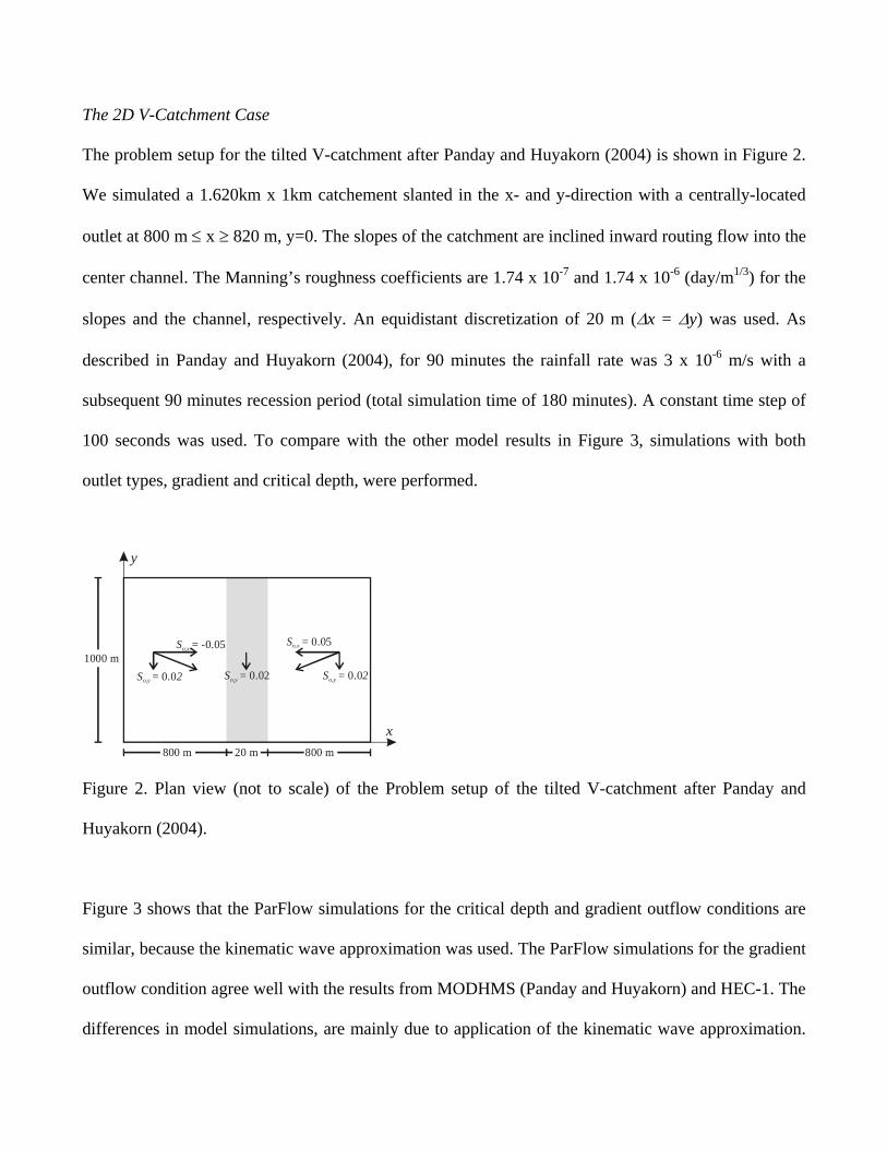
The 2D V-Catchment Case
The problem setup for the tilted V-catchment after Panday and Huyakorn (2004) is shown in Figure 2.
We simulated a 1.620km x 1km catchement slanted in the x- and y-direction with a centrally-located
outlet at 800 m ≤ x ≥ 820 m, y=0. The slopes of the catchment are inclined inward routing flow into the
center channel. The Manning’s roughness coefficients are 1.74 x 10⁻⁷ and 1.74 x 10⁻⁶ (day/m1/3) for the
slopes and the channel, respectively. An equidistant discretization of 20 m (∆x = ∆y) was used. As
described in Panday and Huyakorn (2004), for 90 minutes the rainfall rate was 3 x 10⁻⁶ m/s with a
subsequent 90 minutes recession period (total simulation time of 180 minutes). A constant time step of
100 seconds was used. To compare with the other model results in Figure 3, simulations with both
outlet types, gradient and critical depth, were performed.
So,x = -0.05 So,x = 0.051000 m
800 m 20 m 800 m
So,y = 0.02S 2o,y = 0.0 S 2o,y = 0.0
x
y
Figure 2. Plan view (not to scale) of the Problem setup of the tilted V-catchment after Panday and
Huyakorn (2004).
Figure 3 shows that the ParFlow simulations for the critical depth and gradient outflow conditions are
similar, because the kinematic wave approximation was used. The ParFlow simulations for the gradient
outflow condition agree well with the results from MODHMS (Panday and Huyakorn) and HEC-1. The
differences in model simulations, are mainly due to application of the kinematic wave approximation.
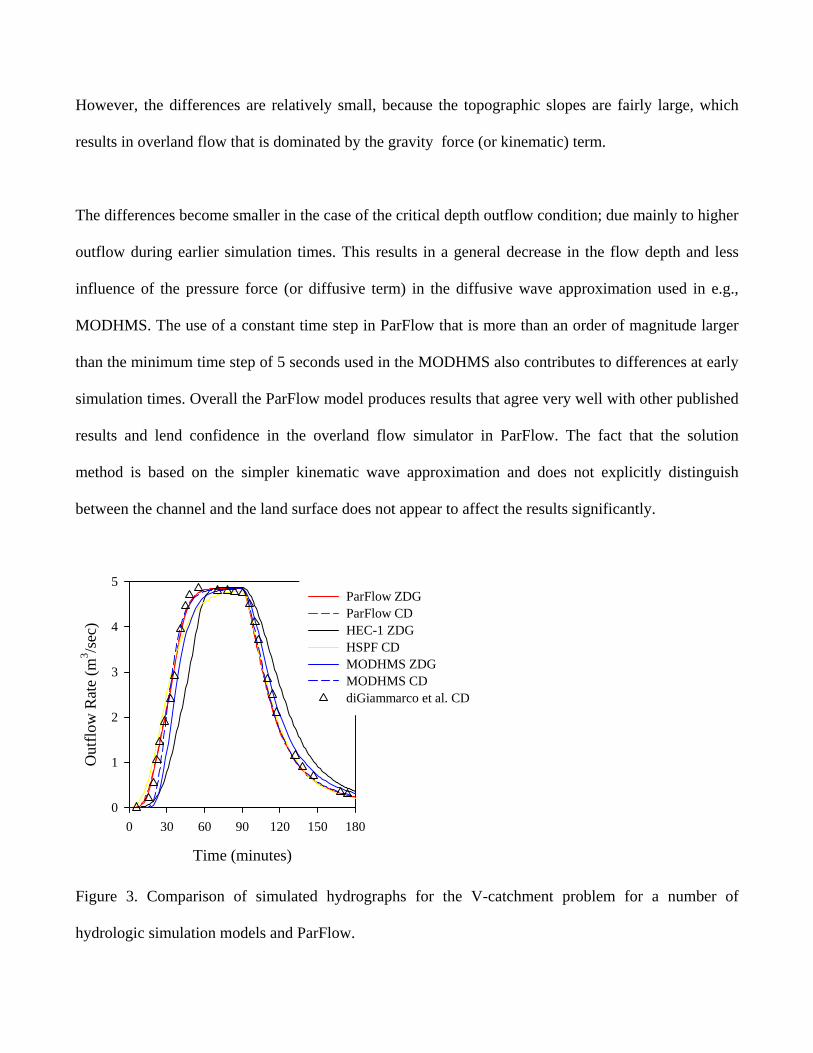
However, the differences are relatively small, because the topographic slopes are fairly large, which
results in overland flow that is dominated by the gravity force (or kinematic) term.
The differences become smaller in the case of the critical depth outflow condition; due mainly to higher
outflow during earlier simulation times. This results in a general decrease in the flow depth and less
influence of the pressure force (or diffusive term) in the diffusive wave approximation used in e.g.,
MODHMS. The use of a constant time step in ParFlow that is more than an order of magnitude larger
than the minimum time step of 5 seconds used in the MODHMS also contributes to differences at early
simulation times. Overall the ParFlow model produces results that agree very well with other published
results and lend confidence in the overland flow simulator in ParFlow. The fact that the solution
method is based on the simpler kinematic wave approximation and does not explicitly distinguish
between the channel and the land surface does not appear to affect the results significantly.
Time (minutes)
0 30 60 90 120 150 180
Out
flow
Rat
e (m
3 /sec
)
0
1
2
3
4
5ParFlow ZDGParFlow CDHEC-1 ZDG HSPF CD MODHMS ZDG MODHMS CD diGiammarco et al. CD
Figure 3. Comparison of simulated hydrographs for the V-catchment problem for a number of
hydrologic simulation models and ParFlow.
Comparison with 1D Analytical Solution
There exist few analytical solutions for overland flow problems. The one compared to here (e.g.,
Gotardi and Venetulli, 1993) is for a one dimensional channel of constant slope and roughness. The
parameters used in this comparison were obtained from Gotardi and Venetulli (1993) and Jaber and
Mohtar (2003) and are as follows: Sox = 0.0005, n = 2.3 x 10⁻⁷ (day/m1/3), and qr = 0.33 (mm/min).
Rainfall, qr, was applied for 200 minutes followed by 100 minutes of recession (qr = 0), which resulted
in 300 minutes total simulation time. The time step size was constant at 180 sec, as was the spatial
discretization, ∆x = 80 m. There were five cells in the x-direction (nx = 5) resulting in a total flow
length of 400 m. The flow outlet was located at x = 0 and was simulated as a gradient outlet. For the
remainder of the section this particular simulation is referred to as the base case.
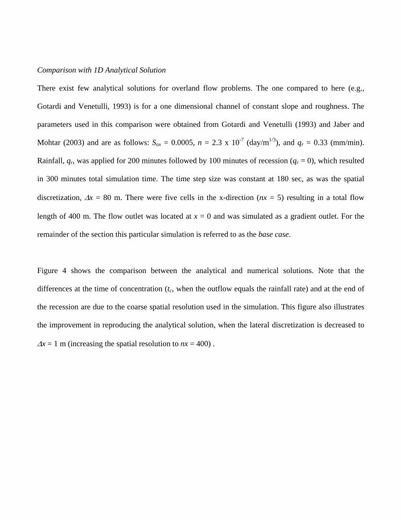
Figure 4 shows the comparison between the analytical and numerical solutions. Note that the
differences at the time of concentration (tc, when the outflow equals the rainfall rate) and at the end of
the recession are due to the coarse spatial resolution used in the simulation. This figure also illustrates
the improvement in reproducing the analytical solution, when the lateral discretization is decreased to
∆x = 1 m (increasing the spatial resolution to nx = 400) .
Time (minutes)
0 50 100 150 200 250 300
Out
flow
rate
(m2 /s
ec)
0.0000
0.0005
0.0010
0.0015
0.0020
0.0025
AnalyticalΝumerical, ∆x = 1 mNumerical, ∆x = 80 m
tc
Figure 4. Comparison between the numerical (symbols) and analytical solution (solid line) for two
different ∆x values.
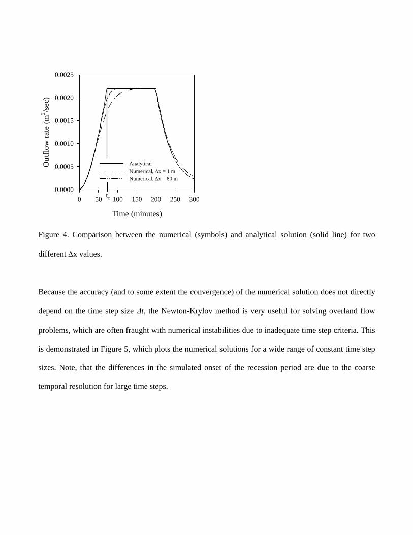
Because the accuracy (and to some extent the convergence) of the numerical solution does not directly
depend on the time step size ∆t, the Newton-Krylov method is very useful for solving overland flow
problems, which are often fraught with numerical instabilities due to inadequate time step criteria. This
is demonstrated in Figure 5, which plots the numerical solutions for a wide range of constant time step
sizes. Note, that the differences in the simulated onset of the recession period are due to the coarse
temporal resolution for large time steps.
Time (minutes)
0 50 100 150 200 250 300
Out
flow
rate
(m2 /s
ec)
0.0000
0.0005
0.0010
0.0015
0.0020
0.0025
∆t = 90 sec∆t = 180 sec ∆t = 360 sec ∆t = 720 sec
Figure 5. The effect of time step size on simulated outflow for the 1-D overland flow problem.
3.2 Integrated modeling examples
In this section we present simulations that focus on the interaction of flow between the surface and
subsurface. The runoff generating processes of excess saturation and infiltration are examined and
compared to the 1D base case. The influence of vertical spatial discretization and subsurface
heterogeneity in the hydraulic conductivity on the resulting hydrograph are also investigated. In all
cases the gradient outlet condition is employed and a constant rainfall rate of qr = 0.33 (mm/min) is
applied for 200 minutes followed by 100 minutes of recession. Table 1 provides a summary of the
different simulations.
Table 1. Summary of the integrated modeling examples.
Type WT depth (m) ∆z (m) Ksat (m/day) 0.2 1.0 0.05 0.2
Excess saturation Ksat > qr
0.5 0.05
1.0
0.05 0.01
0.1
0.05
Excess infiltration Ksat < qr
1.0
0.01 0.01
1.0, slab: 0.01 Mixed 1.0 0.05 Kg = 0.4752 σ[ln(Ksat)] = 3.0
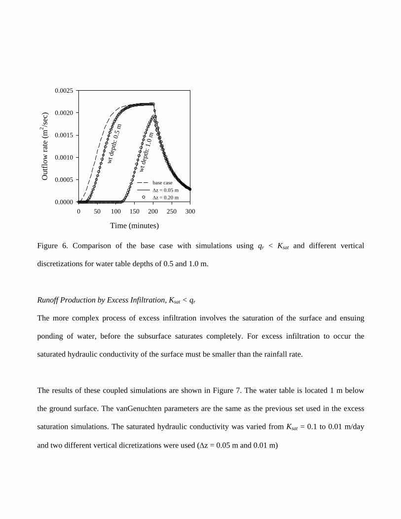
Runoff Production by Excess Saturation, Ksat > qr
The process of excess saturation simply involves the complete saturation of the subsurface and the
intersection of the land surface by the water table, where the outcroping water table produces the
runoff. To accomplish this, the hydraulic conductivity must be larger than the rainfall rate. We
simulated two cases with a shallow water table located at a depth of 0.5 m and 1.0 m below the ground
surface. The vanGenuchten parameters and saturated hydraulic conductivity are as follows: Ksat = 1.0
m/day, N = 2.0, α = 1.0, θres = 0.08, θsat = 0.4. The results of these two cases are shown in Figure 6.
Additionally, for each case, the sensitivity of runoff to the vertical discretization was explored. This
was achieved by varying the constant vertical discretization from ∆z = 0.05 m to ∆z = 0.2 m. Figure 6
also shows the results from the base case for comparison. For excess saturation, Figure 6 reveals, that
the vertical discretization does not have a significant impact on the predicted outflow hydrograph. This
can be seen by comparing the curves using different ∆z values for a given water table depth. For the
water table depth of 0.5 m and 1 m, the times of ponding are some 19 minutes and 117 minutes,
respectively. For the 1 m initial water table depth, no steady state is reached and the outflow rate is
always smaller than rainfall rate multiplied by the length of the channel.
Time (minutes)
0 50 100 150 200 250 300
Out
flow
rate
(m2 /s
ec)
0.0000
0.0005
0.0010
0.0015
0.0020
0.0025
base case∆z = 0.05 m∆z = 0.20 m
wt d
epth
: 1.0
m
wt d
epth
: 0.5
m
Figure 6. Comparison of the base case with simulations using qr < Ksat and different vertical
discretizations for water table depths of 0.5 and 1.0 m.
Runoff Production by Excess Infiltration, Ksat < qr
The more complex process of excess infiltration involves the saturation of the surface and ensuing
ponding of water, before the subsurface saturates completely. For excess infiltration to occur the
saturated hydraulic conductivity of the surface must be smaller than the rainfall rate.
The results of these coupled simulations are shown in Figure 7. The water table is located 1 m below
the ground surface. The vanGenuchten parameters are the same as the previous set used in the excess
saturation simulations. The saturated hydraulic conductivity was varied from Ksat = 0.1 to 0.01 m/day
and two different vertical dicretizations were used (∆z = 0.05 m and 0.01 m)
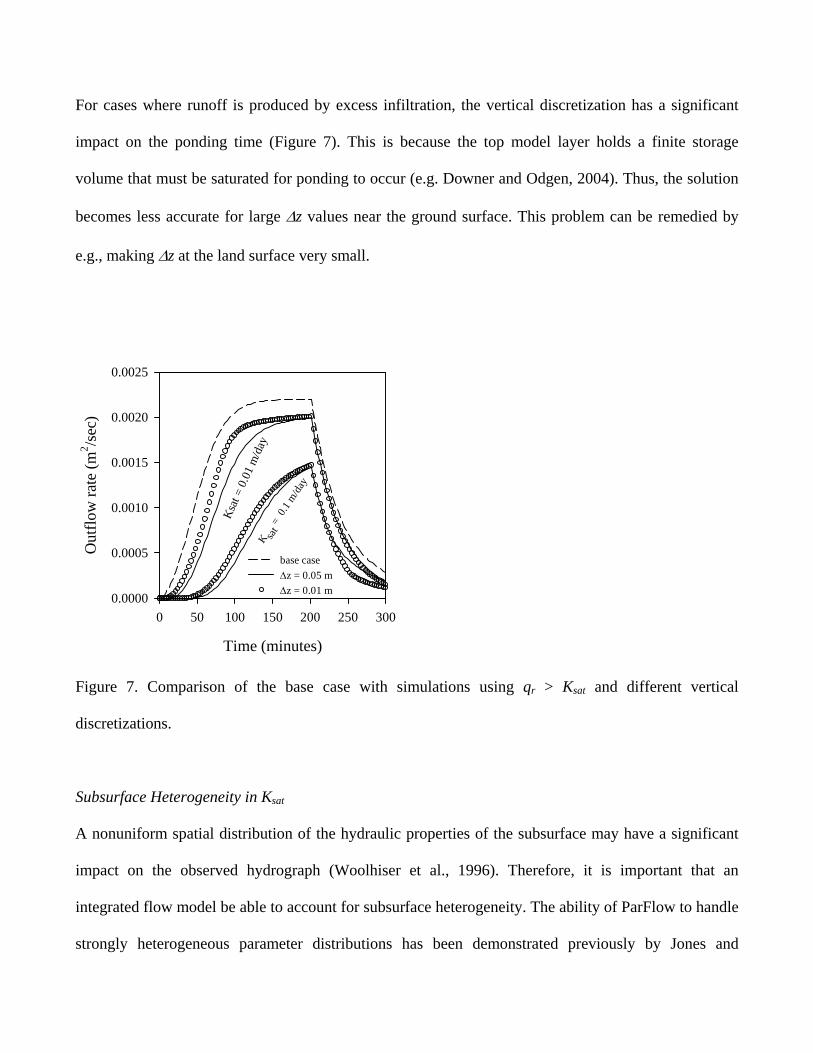
For cases where runoff is produced by excess infiltration, the vertical discretization has a significant
impact on the ponding time (Figure 7). This is because the top model layer holds a finite storage
volume that must be saturated for ponding to occur (e.g. Downer and Odgen, 2004). Thus, the solution
becomes less accurate for large ∆z values near the ground surface. This problem can be remedied by
e.g., making ∆z at the land surface very small.
Time (minutes)
0 50 100 150 200 250 300
Out
flow
rate
(m2 /s
ec)
0.0000
0.0005
0.0010
0.0015
0.0020
0.0025
base case∆z = 0.05 m∆z = 0.01 m
K sat =
0.1
m/day
Ksat
= 0.
01 m
/day
Figure 7. Comparison of the base case with simulations using qr > Ksat and different vertical
discretizations.
Subsurface Heterogeneity in Ksat
A nonuniform spatial distribution of the hydraulic properties of the subsurface may have a significant
impact on the observed hydrograph (Woolhiser et al., 1996). Therefore, it is important that an
integrated flow model be able to account for subsurface heterogeneity. The ability of ParFlow to handle
strongly heterogeneous parameter distributions has been demonstrated previously by Jones and
Woodward (2001), Tompson et al. (1999) and Maxwell et al. (2003) for subsurface flow only. The
following two examples will demonstrate the usefulness of this modeling approach in simulating
interactions between surface water and groundwater under heterogeneous subsurface conditions.
The first example is a variation of the excess saturation case described above. The difference is the
inclusion of a 100 m long, low conductivity slab, Ksat = 0.01 m/day, located in the center of the domain
extending from the land surface to a depth of 0.05m. The initial water table was set to a depth of 1.0 m
below the land surface and the vertical discretization was ∆z = 0.05 m. Figure 8 shows the resulting
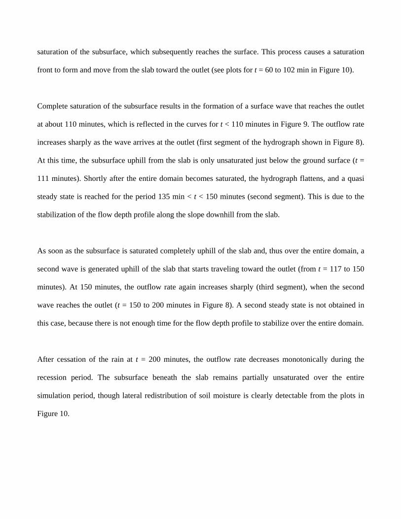
hydrograph and a comparison with the base and the homogeneous excess saturation case.
The simulated hydrograph is characterized by four distinct segments: two steep segments separated by
a flat segment and a recession period after cessation of the rain (at t=200 minutes), which makes up the
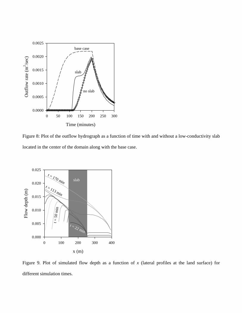
fourth segment. Figure 9 shows the temporal evolution of the flow depth distribution at the land
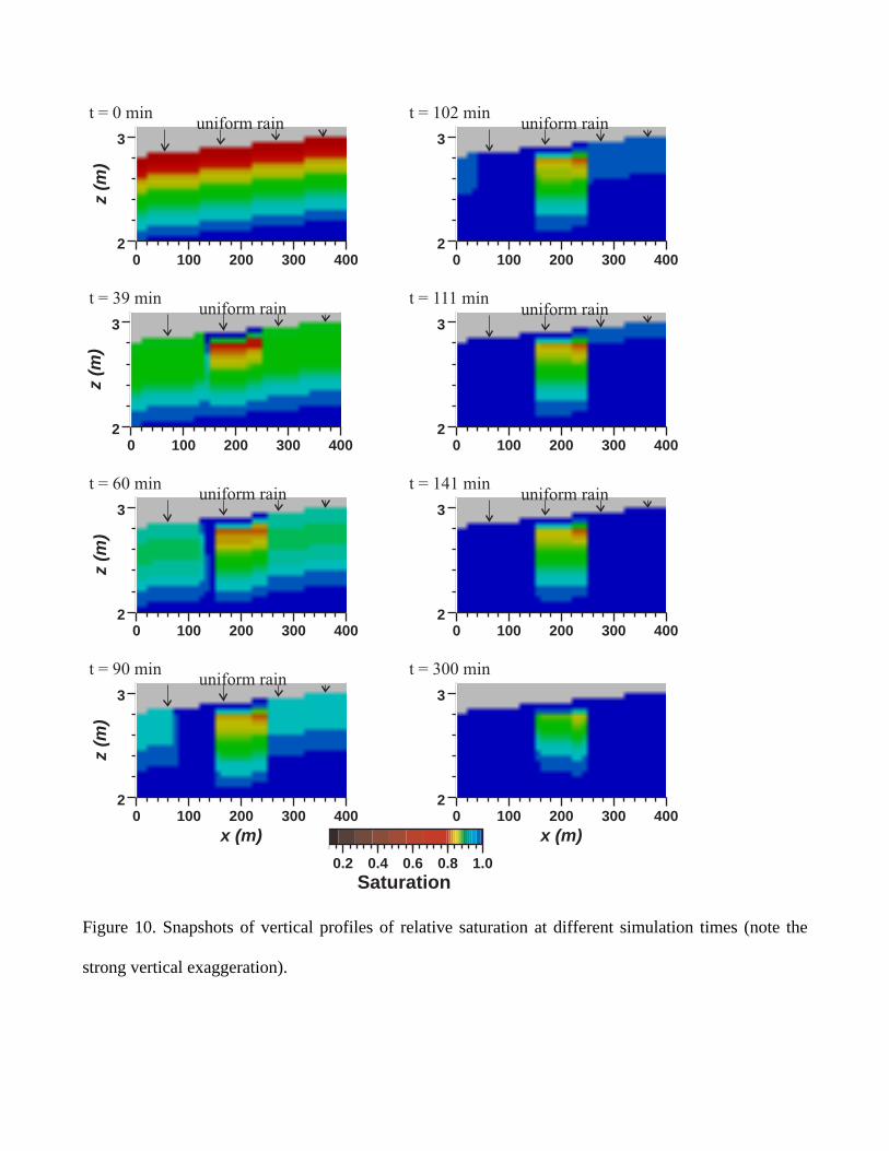
surface. Figure 10 contains a time series of plots of the vertical relative saturation profiles of the
domain starting from the initial conditions at t = 0. The step-like representation of the topography in
ParFlow (e.g., Figure 10) is a result of the lateral discretization, the topographic slope and the finite
difference grid. Figures 8 to 10 demonstrate the interactions and interdependence of excess infiltration
and saturation processes in the presence of subsurface heterogeneity and are discussed in detail below.
The time series in Figure 10 (t = 39 min) shows that ponding first occurs in the region of the low-Ksat
slab, because of excess infiltration. This is also illustrated by the flow depth distribution in Figure 9 at
early times. The ponded water is routed over the slab and infiltrates downhill of the slab causing
saturation of the subsurface, which subsequently reaches the surface. This process causes a saturation
front to form and move from the slab toward the outlet (see plots for t = 60 to 102 min in Figure 10).
Complete saturation of the subsurface results in the formation of a surface wave that reaches the outlet
at about 110 minutes, which is reflected in the curves for t < 110 minutes in Figure 9. The outflow rate
increases sharply as the wave arrives at the outlet (first segment of the hydrograph shown in Figure 8).
At this time, the subsurface uphill from the slab is only unsaturated just below the ground surface (t =
111 minutes). Shortly after the entire domain becomes saturated, the hydrograph flattens, and a quasi
steady state is reached for the period 135 min < t < 150 minutes (second segment). This is due to the
stabilization of the flow depth profile along the slope downhill from the slab.
As soon as the subsurface is saturated completely uphill of the slab and, thus over the entire domain, a
second wave is generated uphill of the slab that starts traveling toward the outlet (from t = 117 to 150
minutes). At 150 minutes, the outflow rate again increases sharply (third segment), when the second
wave reaches the outlet (t = 150 to 200 minutes in Figure 8). A second steady state is not obtained in
this case, because there is not enough time for the flow depth profile to stabilize over the entire domain.
After cessation of the rain at t = 200 minutes, the outflow rate decreases monotonically during the
recession period. The subsurface beneath the slab remains partially unsaturated over the entire
simulation period, though lateral redistribution of soil moisture is clearly detectable from the plots in
Figure 10.
Time (minutes)
0 50 100 150 200 250 300
Out
flow
rate
(m2 /s
ec)
0.0000
0.0005
0.0010
0.0015
0.0020
0.0025base case
slab
no slab
Figure 8: Plot of the outflow hydrograph as a function of time with and without a low-conductivity slab
located in the center of the domain along with the base case.
x (m)
0 100 200 300 400
Flow
dep
th (m
)
0.000
0.005
0.010
0.015
0.020
0.025
slab
t = 22 min
t = 5
0 m
in
t = 113 min
t = 170 min
Figure 9. Plot of simulated flow depth as a function of x (lateral profiles at the land surface) for
different simulation times.
2
3
z (m
)0 100 200 300 400
x (m)
2
3
z (m
)
0 100 200 300 400x (m)
2
3
z (m
)
0 100 200 300 400x (m)
2
3
z (m
)
0 100 200 300 400x (m)
2
3
z (m
)
0 100 200 300 400x (m)
2
3
z (m
)
0 100 200 300 400x (m)
2
3
z (m
)
0 100 200 300 400x (m)
2
3
z (m
)
0 100 200 300 400x (m)
0.2 0.4 0.6 0.8 1.0Saturation
Figure 10. Snapshots of vertical profiles of relative saturation at different simulation times (note the
strong vertical exaggeration).
The second heterogeneous example consists of a set of simulations, where each simulation is based on
a realization of random subsurface heterogeneity in Ksat. We used a hypothetical, correlated Gaussian
random field to describe the distribution of the saturated hydraulic conductivity (Tompson et al., 1989)
with the following properties: geometric mean: Kg = 0.4752 m/day; standard deviation: σ[ln(k)] = 3.0;
correlation lengths in horizontal and vertical direction, respectively: ηh = 50.0 m, ηz = 1.0 m. Different
random seeds were used to generate four equally likely realizations of the Ksat distribution. Note that
the geometric mean of the distribution is equal the rainfall rate. This allows both runoff-generating
processes (excess saturation and infiltration) to occur simultaneously in the simulations. The spatial
distribution of these processes depends on the lateral Ksat distribution in the top layer of an individual
realization. The initial water table depth was set at 1.0 m. The horizontal and vertical discretizations
were 10 m and 0.05 m, respectively to capture the scale of the heterogeneity and the infiltration excess
timing. For comparison, the model was also run for a homogeneous saturated hydraulic conductivity,
Ksat = Kg = 0.4752 m/d, referred to below as the geometric mean simulation.
Figure 11 shows the hydrographs for four realizations of subsurface heterogeneity, the geometric mean
simulation, and the base case. The spread in the curves for the different realizations is a measure of the
uncertainty associated with the hydrograph due to uncertainty in the subsurface heterogeneity. Because
all other parameters were kept constant and the rainfall rate was applied uniformly in space, this figure
illustrates the direct impact of subsurface heterogeneity on the outflow rate. Comparing the geometric
mean simulation with the different realizations, it can be seen that the geometric mean simulation
underestimates the runoff rate at earlier times (t < 150 minutes), when the process of excess infiltration
plays a dominant role in the production of runoff. For the duration 150 < t > 200 minutes, the geometric
mean simulation is bounded by the set of curves from the different realizations. During this time period
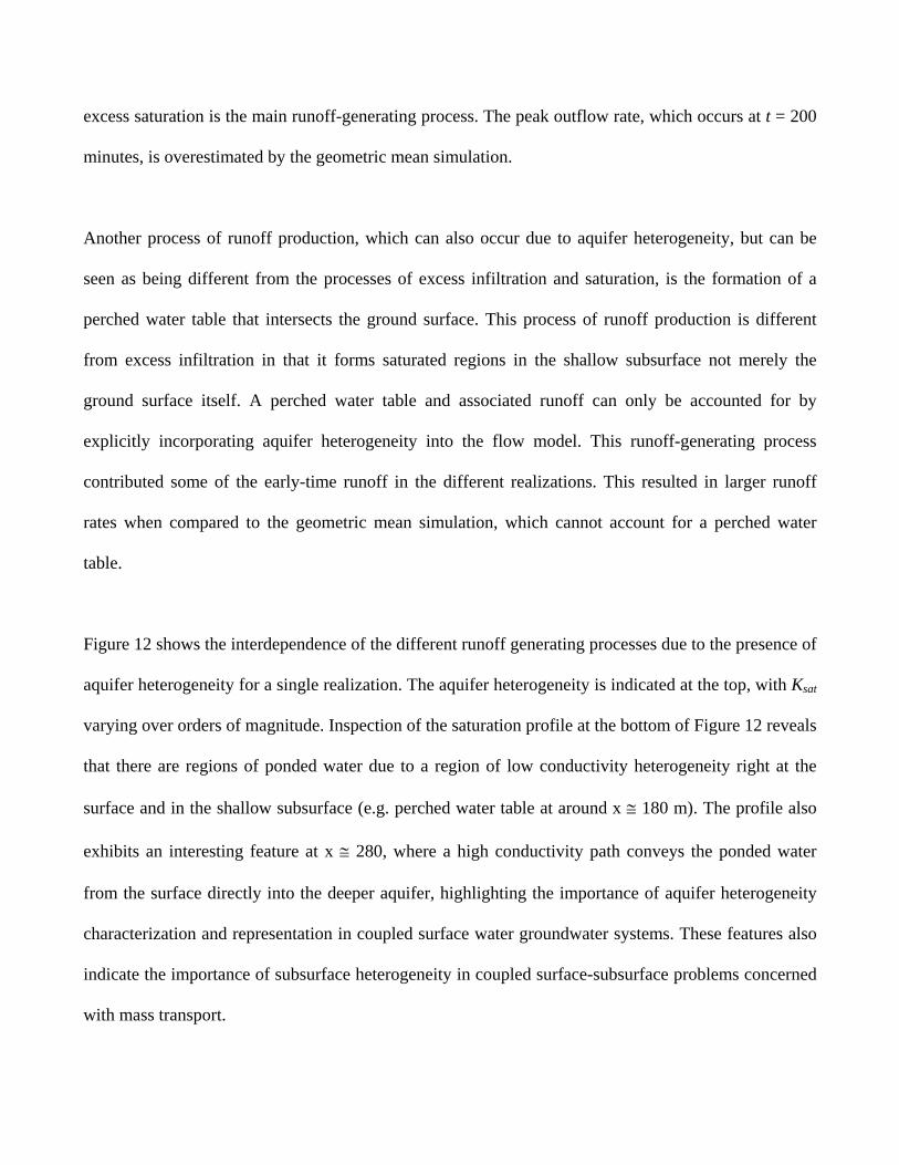
excess saturation is the main runoff-generating process. The peak outflow rate, which occurs at t = 200
minutes, is overestimated by the geometric mean simulation.
Another process of runoff production, which can also occur due to aquifer heterogeneity, but can be
seen as being different from the processes of excess infiltration and saturation, is the formation of a
perched water table that intersects the ground surface. This process of runoff production is different
from excess infiltration in that it forms saturated regions in the shallow subsurface not merely the
ground surface itself. A perched water table and associated runoff can only be accounted for by
explicitly incorporating aquifer heterogeneity into the flow model. This runoff-generating process
contributed some of the early-time runoff in the different realizations. This resulted in larger runoff
rates when compared to the geometric mean simulation, which cannot account for a perched water
table.
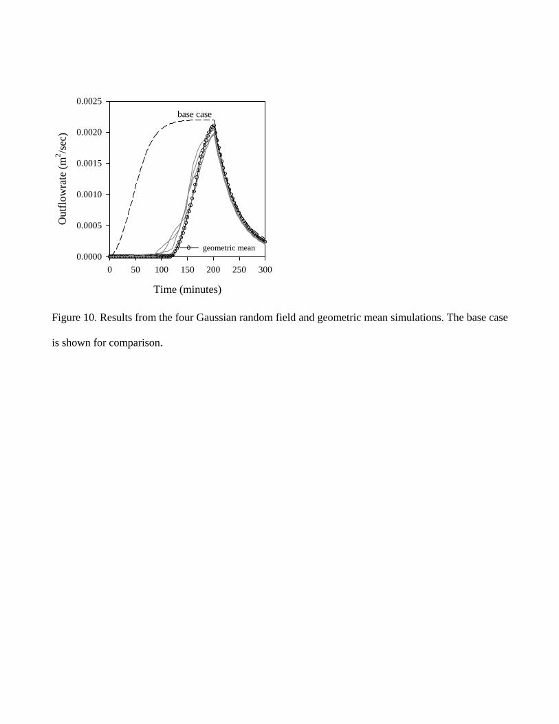
Figure 12 shows the interdependence of the different runoff generating processes due to the presence of
aquifer heterogeneity for a single realization. The aquifer heterogeneity is indicated at the top, with Ksat
varying over orders of magnitude. Inspection of the saturation profile at the bottom of Figure 12 reveals
that there are regions of ponded water due to a region of low conductivity heterogeneity right at the
surface and in the shallow subsurface (e.g. perched water table at around x ≅ 180 m). The profile also
exhibits an interesting feature at x ≅ 280, where a high conductivity path conveys the ponded water
from the surface directly into the deeper aquifer, highlighting the importance of aquifer heterogeneity
characterization and representation in coupled surface water groundwater systems. These features also
indicate the importance of subsurface heterogeneity in coupled surface-subsurface problems concerned
with mass transport.
Time (minutes)
0 50 100 150 200 250 300
Out
flow
rate
(m2 /s
ec)
0.0000
0.0005
0.0010
0.0015
0.0020
0.0025
geometric mean
base case
Figure 10. Results from the four Gaussian random field and geometric mean simulations. The base case
is shown for comparison.
2
3
z (m
)
0 100 200 300 400x (m)
-3 -2 -1 0 1 2log(K)
2
3
z (m
)
0 100 200 300 400x (m)
0.2 0.4 0.6 0.8 1.0Saturation
Figure 12. Example of a Ksat distribution of a single realization (top) and the associated relative
saturation profile after 45 minutes simulation time (bottom).
Parallel Scalability
A major advantage of ParFlow over other existing integrated hydrologic modeling tools is the
infrastructure devised for massively parallel computer systems (Ashby and Falgout, 1996; Jones and
Woodward, 2001). The overland flow simulator discussed here is designed to exploit this infrastructure
and is, thus, massively parallel as well. A determining factor of parallel efficiency is the time the code
spends on inter-processor communications (communication overhead) relative to the computation time.
When the ratio between communication overhead and computation time is small, the parallel efficiency
is large. Parallel efficiency of the overland flow simulator in ParFlow was studied by performing
simulations of varying problem sizes and analyzing the respective run times. Following Jones and
Woodard (2001) the scaled efficiency, E, is defined as E(np,p) = T(n,1) / T(np,p), where T is the run
time as a function of the problem size, n; and the number of processors, p. For the case of a perfectly
efficient parallel simulator, E(np,p) = 1, doubling the problem size and the number of processors will
result in the same run time.
Figure 13 shows E for two different modeling problems: overland flow only (surface) and for the case
of excess infiltration produced runoff (surface/subsurface). The two different problems were run for a
smaller number of model cells (nx,ny,nz) per processor (20,20,1 and 20,20,5) and for are larger number
(100,100,1 and 100,100,5) to test the performance of the code for different communication overhead
and computation time ratios.
For the smaller problem size, the parallel efficiency of the excess infiltration case is significantly higher
than for the overland flow only case. The scaled efficiency for the excess infiltration case levels off at
about 0.60, whereas the scaled efficiency for the overland flow only case levels off at about 0.45. This
is due to relatively small computational times at individual processors for the overland flow only case
and, thus, large communication overhead versus computation time ratios.
This trend, however, is reversed when the problem size at each processor is increased to 100,100,1 and
100,100,5. Figure 13 shows a significant increase in the scaled efficiency for the overland flow only
case, which now levels of at about 0.82. An increase, though smaller, is also observed in the saturation
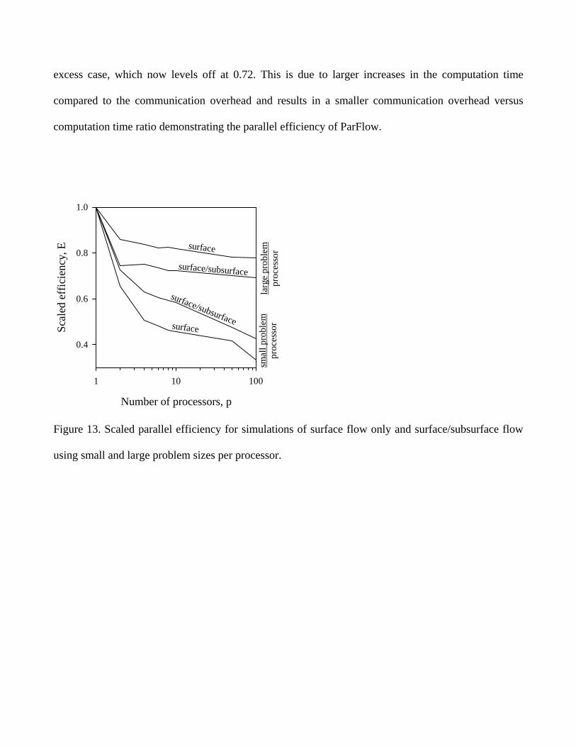
excess case, which now levels off at 0.72. This is due to larger increases in the computation time
compared to the communication overhead and results in a smaller communication overhead versus
computation time ratio demonstrating the parallel efficiency of ParFlow.
Number of processors, p
1 10 100
Scal
ed e
ffic
ienc
y, E
0.4
0.6
0.8
1.0
smal
l pro
blem
proc
esso
rsurface/subsurface
surface/subsurface
surface
surface
larg
e pr
oble
mpr
oces
sor
Figure 13. Scaled parallel efficiency for simulations of surface flow only and surface/subsurface flow
using small and large problem sizes per processor.
4 Conclusions
A new formulation of coupled surface water groundwater flow, which does not depend on a
conductance-like relationship, has been described. This formulation forms the basis of an overland flow
simulator based on the kinematic wave approximation, that has been implemented in the parallel, three-
dimensional, variable saturated flow code ParFlow. The overland flow simulator takes the form of a
free-surface upper boundary condition for the problem of variable saturated groundwater flow and is
therefore fully integrated.
The overland flow simulator was verified using previously published data and an analytical solution.
The globalized Newton solution methods allow for the application of very large time steps without
compromising numerical stability, which is an advantage over other approaches that are based on
restricting stability criteria. Simulation examples were presented that focused on the two main
processes of runoff production, excess saturation and infiltration. The effect of varying vertical
discretization was also studied. Changes in the vertical discretization had a significant impact on the
solution only in the case of excess infiltration, due to dependence of the time of ponding on the finite
storage of the top layer.
We have shown that shallow subsurface heterogeneity may have a strong influence on the outflow rate
and may cause a segmented hydrograph. A set of simulations where a heterogeneous subsurface was
simulated as a correlated random field was used to demonstrate how uncertainty due to subsurface
heterogeneity influences uncertainty in runoff predictions. A comparison with a homogeneous
geometric mean simulation of the hydraulic conductivity showed that the geometric mean simulation
may not account for excess infiltration and thus underestimates early parts of the hydrograph. Because
the new coupled formulation can explicitly account for subsurface heterogeneity, the production of
runoff due to the formation of a perched water table can be simulated. This process of runoff
production is generally neglected by other hydrologic modeling tools and acts on a time scale between
excess infiltration (short time scale) and excess saturation (long to very long time scale) depending on
the depth of the water table from the ground surface.
A parallel efficiency study showed the excellent scalability of the overland flow simulator and the
fully-coupled surface-subsurface simulator for large problems. This makes this new coupled model
especially suitable for small and large watershed modeling, where the efficient use of large
computational resources is vital.
5 Acknowledgements
This work was conducted under the auspices of the U. S. Department of Energy by the University of
California, Lawrence Livermore National Laboratory (LLNL) under contract W-7405-Eng-48. This work
was funded by DOE Fossil Energy Program NETL, NPTO, Tulsa, OK and by the LLNL OPC program.
We are especially indebted to S. Panday for providing the original data for Figure 3 and Andrew
Tompson for the constructive discussions.
5 References
Anderson MP, Woessner WW. Applied groundwater modeling: simulation of flow and advective
transport. Academic Press, San Diego 1992; p. 281.
Ashby SF, Falgout RD. A parallel multigrid preconditioned conjugate gradient algorithm for
groundwater flow simulations. Nucl Sci Eng 1996;124(1):145-59.
Bicknell BR, Imhoff JL, Kittle JL, Donigian AS, Johanson RC. Hydrologic Simulation Program
FORTRAN (HSPF): User’s Manual for Release 10, EPA-600/R-93/174, US Environmental
Protection Agency, Athens, GA, 1936.
Braunschweig, F., P.C. Leitao, L. Fernandes, P.Pina and R.J.J. Neves. The object-oriented design of the
integrated water modelling system MOHID. Proceedings of the XV International Conference on
Computation Methods in Water Resources (CMWR XV), Chapel Hill, NC, USA, Elsevier,
2004; 2:1079-90.
Cardenas MBR, Zlontik VA. Three-dimensional model of modern channel bend deposits. Water
Resour Res 2003;39(6),1141,doi:10.1029/2002WR001383.
Downer CW, Odgen FL. Appropriate vertical discretization of Richards’ equation for two-dimensional
watershed-scale modeling. Hydrol. Process. 2004;18:1-22.
Fiedler FR, Ramirez JA. A numerical method for simulating discontinous shallow flow over an
inifltrating surface. Int J Numer Meth Fluids 2000;32:219-40.
Forsyth PA, Wu YS, Pruess K. Robust numerical methods for saturated-unsaturated flow with dry
conditions in heteroegeneous media. Adv. Water Resour 1995;18:25-38.
Freeze, R.A. and R.L. Harlan. Blue-print for a physically-based digitally simulated hydrologic response
model. J Hydrol. 1960; 9, 237-58.
Gottardi G, Venutelli M. A control-volume finite element model for two dimensional overland flow.
Adv Water Resour 1993;16:227-84.
Govindaraju RS and Kavvas ML. Dynamics of moving boundary overland flows over infiltrating
surfaces at hillslopes Water Resour Res 1991; 27(8), 1885-98.
Gunduz O and Mustafa MA. River networks and groundwater flow: a simultaneous solution of
acoupled system. J Hydrol 2005;301:216-34.
Hantush MS. Wells near streams with semipervious beds. J Geophys Res 1965;70:2829-38.
Huyakorn PS, Springer EP, Guvanasen V, Wadsworth TD. A three dimensional finite element model
for simulating water flow in variable saturated porous media. Water Resour Res
1986;22(12):1790-808.
Huyakorn, P. S. and G.F. Pinder, Computational Methods In Subsurface Flow, New York: Academic
Press, 1983.
Jaber FH, Mohtar RH. Stability and accuracy of two-dimensional kinematic wave overland flow
modeling. Adv Water Resour 2003;26;1189-98.
Jones JE, Woodward CS. Newton-Krylov-multigrid solvers for large-scale, highly heterogeneous,
variable saturated flow problems. Adv Water Resour 2001;24:763-74.
Jones JE, Woodward CS. Preconditioning Newton-Krylov methods for baribale saturated flow. In:
Bentley LR, Sykes JF, Brebbia CA, Gray WG, Pinder GF, editors. Computational methods in
water resources, vol. 1. Balkema: Rotterdam; 2000. p. 101-6.
Kirkland MR, Hills RG, Wierenga PJ. Algorithms for solving Richards’ equation for nonuniform
porous media. Water Resour Res 1992; 28:2049-58.
Kollet SJ, Zlontik VA. Stream depletion predictions using pumping test data from a heterogeneous
stream-aquifer system (a case study from the Great Plains, USA). J Hydrol 2003;281:96-114.
Kutilek M, Nielsen DR. Soil Hydrology. Cremlingen-Destedt: Catena –Verl 1994: 370.
Kutilek M, Nielson DR. Soil hyrology. GeoEcology, Catena Verlag, Cremlingen-Destedt, Germany,
1994; p. 370.
LaBolle EM, Ahmed AA, Fogg GE. Review of integrated groundwater and surface water model
(IGSM). Ground Water 2003;41(2):238-46.
Maxwell RM, Welty C, Tompson AFB. Streamline-based simulation of virus transport resulting from
long term artificial recharge in a heterogeneous aquifer. Adv Water Resour 2003;25(10):1075-
96.
Miller CT, Williams GA, Kelley CT, Tocci MD. Robust solution of Richards’ equation for nonuniform
porous media. Water Resour Res 1998;34:2599-610.
Moench, A. Flow to a well of finite diameter in a homogeneous, anisotropic water table aquifer. Water
Resour Res 1997;33(6):1397-407.
Neuman SP. Theory of flow in unconfined aquifers considering dealyed aquifer response. Water
Resour Res 1972;8(4):1031-44.
Panday S, Huyakorn PS. A fully coupled physically-based spatially-distributed model for evaluating
surface/subsurface flow. Adv Water Resour 2004;27:361-82.
Putti, M and C. Paniconi. Time step and stability control for a coupled model of surface and subsurface
flow. Proceedings of the XV International Conference on Computation Methods in Water
Resources (CMWR XV), Chapel Hill, NC, USA, Elsevier, 2004; 2:1391-1402.
Saad Y. Iterative methods for sparse linear systems. 2nd edition, SIAM, Philladelphia, 2003.
Taylor C, Al-Mashidani G, Davis JM. A finite element approach to watershed runoff. J Hydrol
1974;21:231-46.
Therrien R, Sudicky EA. Three-dimensional analysis of variable-saturated flow and solute transport in
discretely-fractured porous media. J. Contam. Hydrol. 1996;23:1-44.
Tompson, A.F.B., R. Ababou, and L. Gelhar. Implementation of the 3-dimensional turning bands
random field generator, Water Resour. Res., 1989; 25(10), 2227-43.
Tompson AFB, Carle SF, Rosenberg ND, Maxwell RM. Analysis of groundwater migration from
artificial recharge in a large urban aquifer: A simulation perspective. Water Resour Res
1999;35(10):2981-98.
USACE. HEC-1: Flood Hydrograph Package, User’s Manual, Version 4.1, US Army Corps of
Engineers, Hydrologic Engineering Center, Davis, CA, 1998.
Van Genuchten MTh. A closed-form equation for predicting the hydraulic conductivity of unsaturated
soils. Soil Sci SocAm J 1980;44:892-98.
VanderKwaak JE. Loague K. Hydrologic-response simulations for the R-5 catchment with a
comprehensive phisics-based model. Water Resour Res 2001;37(4):999-1013.
Wallach R, Grigorin G, Rivlin(Byk) J. The errors in surface runoff prerdiction by neglecting the
relationship between infiltration and overland flow depth. J Hydrol 1997;200:243-59.
Woodward CS, Dawson CN. Analysis of expanded mixed finite element methods for a nonlinear
parabolic equation modeling flow into variable staurated porous media. SIAM J Numer Anal
2000;37(3):701-24.
Woolhiser DA, Smith RE, Giraldez JV. Effects of spatial variability of the saturated conductivity on
Hortonian overland fow. Water Resour Res 1996;32(3):671-78.