Integrated Scheduling and Synthesis of Control Applications on Distributed Embedded Systems Soheil...
22
Integrated Scheduling and Synthesis of Control Applications on Distributed Embedded Systems Soheil Samii 1 , Anton Cervin 2 , Petru Eles 1 , Zebo Peng 1 1 Dept. of Computer and Information Science Linköping University Sweden 2 Dept. of Automatic Control Lund University Sweden
-
Upload
marlene-gilbert -
Category
Documents
-
view
216 -
download
1
Transcript of Integrated Scheduling and Synthesis of Control Applications on Distributed Embedded Systems Soheil...
Integrated Scheduling and Synthesis of Control Applications on Distributed
Embedded Systems
Soheil Samii1, Anton Cervin2, Petru Eles1, Zebo Peng1
1 Dept. of Computer and Information Science
Linköping University
Sweden
2 Dept. of Automatic Control
Lund University
Sweden

2
Motivation
• Many embedded control systems are distributed
• Typical example: the modern car
• Timing delays
• Sampling, computation, and actuation
• Sharing of computation and communication resources
• Problem: Degradation of control performance
• System scheduling
• Controller design

3
Outline
• Motivation
• System model
• Example and problem formulation
• Scheduling and synthesis approach
• Experimental results
• Summary and contribution
4
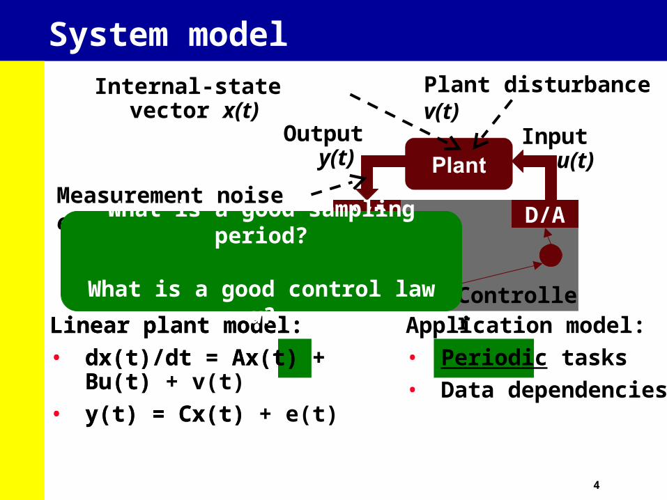
System model
Linear plant model:
• dx(t)/dt = Ax(t) + Bu(t)
• y(t) = Cx(t)
Internal-state vector x(t)
Input u(t)Output y(t)
Measurement noise e(t)
Plant disturbance v(t)
Application model:
• Periodic tasks
• Data dependencies
Linear plant model:
• dx(t)/dt = Ax(t) + Bu(t) + v(t)
• y(t) = Cx(t) + e(t)
Controller
A/D D/AWhat is a good sampling period?
What is a good control law u?

5
Control performance
• Quadratic cost: J = E{ xTQ1x + uTQ2u }
• Depends on
• the sampling period,
• the control law, and
• the distribution of the delay between sampling and actuation of the control signal
• Synthesis of optimal control-law for given
• sampling period and
• constant delay
• Toolbox “Jitterbug”, developed at Lund University in Sweden

6
Example: Control of two pendulums
u
y
u
y
• Measure the angle y
• Stabilize in upright position y=0
• Control the acceleration u of the cart
0 1 0
/ 0.2 0 / 0.2x x u v
g g
1 0y x e
0.2 m0.1 m
J = E{y2 + 0.002u2}

7
Example: Platform
S
A
C
S
A
C
Decide
(1) sampling periods,
(2) design control laws, and
(3) schedule the tasks and messages

8
Example: Ideal control
S
A
C
S
A
C
• Control laws synthesized for the constant delays of each application (9 and 13)
• J1=0.9, J2=2.4, Total=3.3 (achieved for the ideal runtime scenario: dedicated resources)
Sample 20 ms Sample 30 ms
9
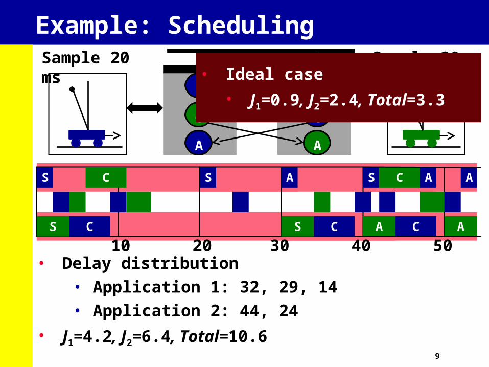
Example: Scheduling
S
A
C
S
A
C
S
CS
C S A
S C
S C
A C
A
A
A
20 4010 30 50• Delay distribution
• Application 1: 32, 29, 14
• Application 2: 44, 24
• J1=4.2, J2=6.4, Total=10.6
Sample 20 ms Sample 30 ms• Ideal case
• J1=0.9, J2=2.4, Total=3.3

10
Example: Scheduling
S
A
C
S
A
C
S
CS
C S A
S C
S C
A C
A
A
A
20 4010 30 50
S
CS
C SA
SC
S C
A C
A
A
A
20 4010 30 50• Delay distribution
• Application 1: 14 (constant)
• Application 2: 18, 24
• J1=1.1, J2=5.6, Total=6.7
Sample 20 ms Sample 30 ms
• Compensate for the delays in the schedule (14 and 21)
• J1=1.0, J2=3.7, Total=4.7
• Ideal case
• J1=0.9, J2=2.4, Total=3.3
• First schedule
• J1=4.2, J2=6.4, Total=10.6

11
Example: Change periods
S
A
C
S
A
C
Sample 30 ms Sample 20 ms
S
CS
C SA
S C
C
A
A
A
20 4010 30 50S
C
A
• Delay distribution
• Application 1: 13, 23
• Application 2: 18
• J1=1.3, J2=2.1, Total=3.4 (with delay compensation)
Good selection of periods combined with integrated
scheduling and control-law synthesis is important!
• With periods 20 ms and 30 ms:
• J1=1.0, J2=3.7, Total=4.7

12
Problem formulation
Available sampling periods
Deadlines
Execution-time specifications
Scheduling and synthesis tool
i iw JPeriods
Control laws
?Minimize

13
Approach (Static-cyclic scheduling)
Select controller periods
Task periods
Schedule the tasks and messages
Delay distributions
Synthesize control-laws and compute cost
Stop?No
Yes Done!
Cost
• Constraint logic programming (CLP)
• Minimize delay and jitter
• CLP solver ”ECLiPSe”
What if we have priority-based scheduling?
• Genetic algorithm for period assignment

14
Approach (Priority-based scheduling)
Select task and message priorities
Synthesize control-laws and compute cost
No
Cost
Delay distributions
Schedulable?
Priorities
SimulateYes
Stop?Yes
CostNo
• Run response-time analysis to obtain worst-case delays
• Bounded delays?
• Deadlines met?
• Genetic algorithm for priority assignment
15
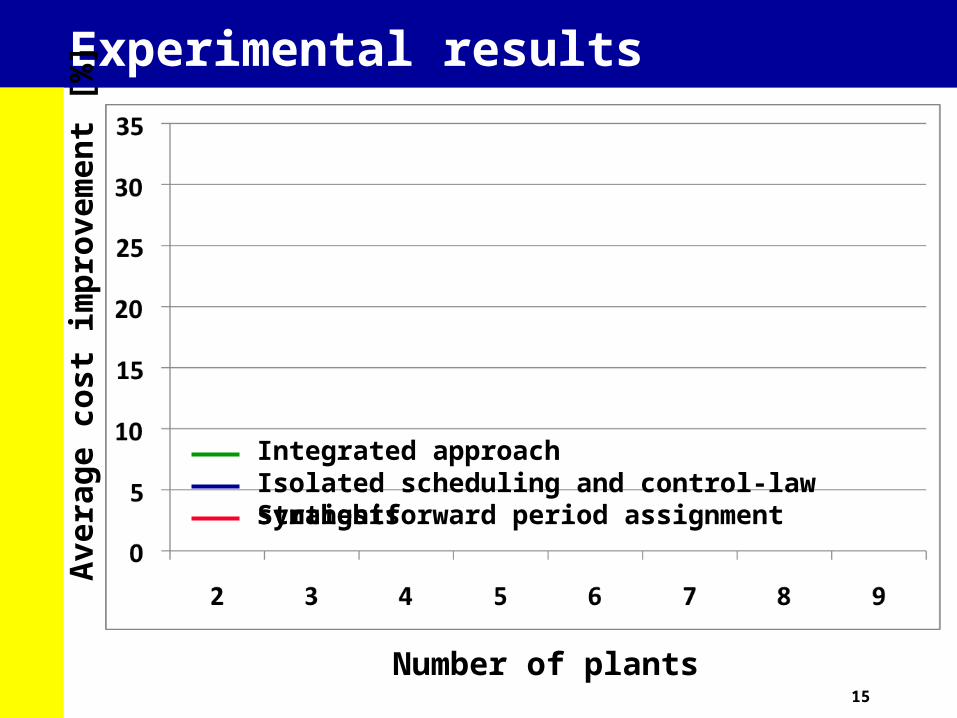
Experimental results
Number of plants
Ave
rag
e co
st i
mp
rove
men
t [%
]
Isolated scheduling and control-law synthesisIntegrated approach
Straightforward period assignment

16
Summary and contribution
• Problem: Sharing of computation and communication resources degrades the control performance
• Solution: Integrate scheduling with control design (period assignment and control-law synthesis)
• Contribution:
• A tool for such integrated design of distributed embedded control systems with
–static-cyclic scheduling or
–priority-based scheduling

17
EXTRA SLIDES
18
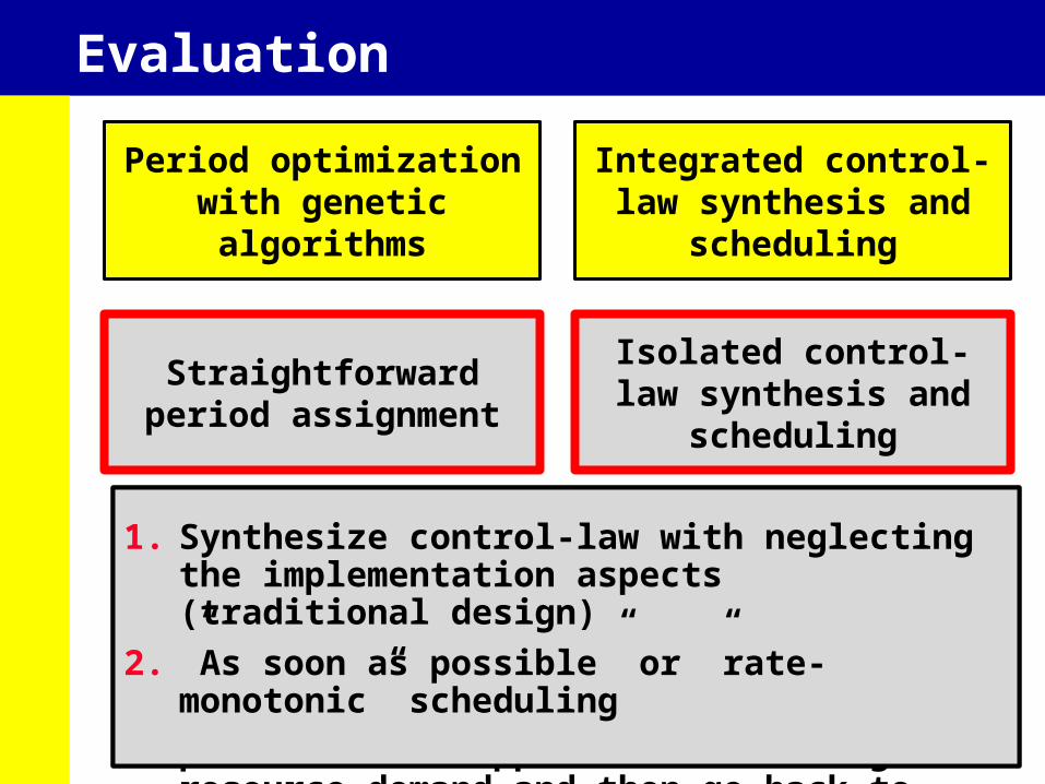
Evaluation
Period optimization with genetic algorithms
Integrated control-law synthesis and
scheduling
Straightforward period assignment
Isolated control-law synthesis and
scheduling
1. Select smallest periods for all applications
2. Schedule system and synthesize control-laws
3. If not schedulable, increase the period of the application with highest resource demand and then go back to Step 2
1. Synthesize control-law with neglecting the implementation aspects (traditional design)
2. ”As soon as possible” or ”rate-monotonic” scheduling

19
Experiments
Period optimization with genetic algorithms
Integrated control-law synthesis and
scheduling
Straightforward period assignment
Isolated control-law synthesis and
scheduling
• Straightforward approach as a baseline, JSF
• Compute relative cost improvement
• (JSF – J) / JSF
• Evaluate each part of the optimization in isolation
• Generated benchmarks with inverted pendulums, servos, and other examples of unstable plants
• 6 to 45 tasks, 2 to 7 computation nodes

20
Static-cyclic scheduling
Number of plants
Ave
rag
e co
st i
mp
rove
men
t [%
]

21
Priority-based scheduling
Number of plants
Ave
rag
e co
st i
mp
rove
men
t [%
]
22
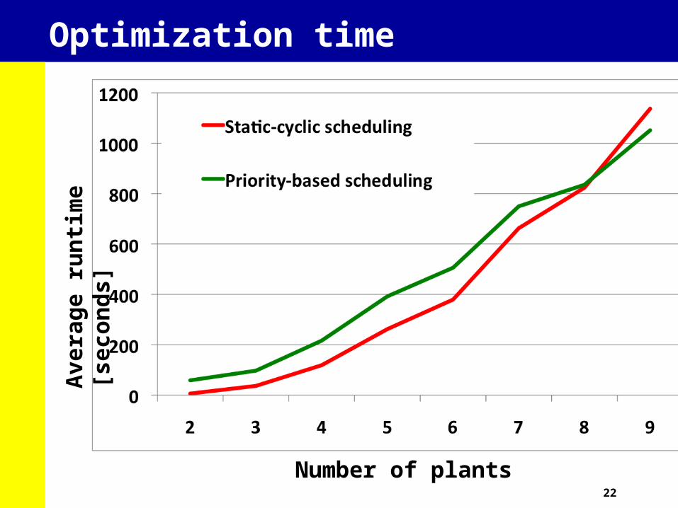
Optimization time
Number of plants
Ave
rag
e ru
nti
me
[sec
on
ds]


![Återkoppling som del i lärandeprocessen Cervin, Anton ...lup.lub.lu.se/search/ws/files/6412631/7761311.pdfProc 31st ACM/SIGCSE Tech Symp on Computer Science Education. [2] Angelo,](https://static.fdocuments.us/doc/165x107/5b1b89607f8b9a3c258ebdd0/aterkoppling-som-del-i-laerandeprocessen-cervin-anton-luplublusesearchwsfiles6412631.jpg)