INTEGRATED RESERVOIR STUDY OF THE MONUMENT …
96
i INTEGRATED RESERVOIR STUDY OF THE MONUMENT NORTHWEST FIELD: A WATERFLOOD PERFORMANCE EVALUATION A Thesis by MOSES ASUQUO NDUONYI Submitted to the Office of Graduate Studies of Texas A&M University in partial fulfillment of the requirements for the degree of MASTER OF SCIENCE December 2007 Major Subject: Petroleum Engineering
Transcript of INTEGRATED RESERVOIR STUDY OF THE MONUMENT …
i
INTEGRATED RESERVOIR STUDY OF THE MONUMENT NORTHWEST
FIELD: A WATERFLOOD PERFORMANCE EVALUATION
A Thesis
by
MOSES ASUQUO NDUONYI
Submitted to the Office of Graduate Studies of Texas A&M University
in partial fulfillment of the requirements for the degree of
MASTER OF SCIENCE
December 2007
Major Subject: Petroleum Engineering
ii
INTEGRATED RESERVOIR STUDY OF THE MONUMENT NORTHWEST
FIELD: A WATERFLOOD PERFORMANCE EVALUATION
A Thesis
by
MOSES ASUQUO NDUONYI
Submitted to the Office of Graduate Studies of Texas A&M University
in partial fulfillment of the requirements for the degree of
MASTER OF SCIENCE
Approved by:
Chair of Committee, David S. Schechter Committee Members, Robert A. Wattenbarger Wayne Ahr Head of Department, Stephen A. Holditch
December 2007
Major Subject: Petroleum Engineering

iii
ABSTRACT
Integrated Reservoir Study of the Monument Northwest Field: A Waterflood
Performance Evaluation. (December 2007)
Moses Asuquo Nduonyi, B.Eng., University of Port Harcourt, Nigeria
Chair of Advisory Committee: Dr. David S. Schechter
An integrated full-field study was conducted on the Monument Northwest field
located in Kansas. The purpose of this study was to determine the feasibility and
profitability of a waterflood using numerical simulation. Outlined in this thesis is a
methodology for a deterministic approach. The data history of the wells in the field
beginning from spud date were gathered and analyzed into information necessary for
building an upscaled reservoir model of the field. Means of increasing production and
recovery from the field via a waterflood was implemented.
Usually, at the time of such a redevelopment plan or scheme to improve field
performance, a tangible amount of information about the reservoir is already known.
Therefore it is very useful incorporating knowledge about the field in predicting future
behavior of the field under certain conditions. The need for an integrated reservoir study
cannot be over-emphasized. Information known about the reservoir from different
segments of the field exploration and production are coupled and harnessed into
developing a representative 3D reservoir model of the field.
An integrated approach is used in developing a 3D reservoir model of the
Monument Northwest field and a waterflood is evaluated and analyzed by a simulation

iv
of the reservoir model. From the results of the reservoir simulation it was concluded that
the waterflood project for the Monument Northwest field is a viable and economic
project.

v
DEDICATION
I dedicate this work to my parents, Nkoyo and Etim Nduonyi, for the
encouragement and love they gave me. I am grateful they believed in me.

vi
ACKNOWLEDGEMENTS
I would like to thank my committee chair, Dr. David Schechter, and my
committee members, Dr. Robert Wattenbarger and Dr. Wayne Ahr for their guidance
and support throughout the course of this research.
I would also like to thank my mentor, Mr. William Johnson, a Reservoir
Engineering Consultant in Kansas for teaching me how to “tie the ropes” the practical
way incorporating the inadequacy of the real world. I am very grateful to Mr. Thomas
Tan of Petrostudies for donating a free license of EXODUS software to the Petroleum
Engineering Department for use in the successful completion of this project. The
software proved to be an invaluable tool.
I thank the faculty and staff of the Petroleum Engineering Department and the
Geology Department; my association with them has been very rewarding in many ways.
I would specifically thank Dr. Christine Economides for teaching me well testing; I
could not have learned it better.
I would also thank Dr. Alan Byrnes of the University of Kansas for sharing
knowledge and information. Thank you for being there always.
Finally, I would like to thank my parents and my brothers for their patience, love,
and support. We all did this project together.
vii
TABLE OF CONTENTS
Page
ABSTRACT .............................................................................................................. iii
DEDICATION .......................................................................................................... v
ACKNOWLEDGEMENTS ...................................................................................... vi
TABLE OF CONTENTS .......................................................................................... vii
LIST OF FIGURES................................................................................................... ix
LIST OF TABLES .................................................................................................... xii
CHAPTER
I INTRODUCTION ............................................................................... 1
Previous Work…………………………………………………… 2
II GEOLOGICAL AND PETROPHYSICAL EVALUATION .............. 4
III DRILL STEM TESTING..................................................................... 15
IV RESERVOIR MODEL DEVELOPMENT.......................................... 22
Deterministic Modeling.................................................................. 22
Porosity Description....................................................................... 23
Permeability Description ………………………………………... 25
Relative Permeability ……………………………………………. 26
Capillary Pressure and Initial Water Saturation …………………. 28
Aquifer Definition ……………………………………………….. 29
Model Initialization and History Matching ……………………… 30 V WATERFLOODING MONUMENT NW FIELD…………………... 42
Layer Subdivision . ........................................................................ 42
viii
........................................................................................................ Page
Selection of Injection Wells ……………………………………... 43
Waterflood Scenarios ……………………………………………. 47
Project Evaluation ……………………………………………….. 51
Monte Carlo Analysis …………………………………………… 54
Conclusions and Recommendations …………………………….. 57
NOMENCLATURE.................................................................................................. 59
REFERENCES.......................................................................................................... 61
APPENDIX A ........................................................................................................... 64
APPENDIX B ……………………………………………………………………... 66
VITA ......................................................................................................................... 84

ix
LIST OF FIGURES
FIGURE Page
1 Flowchart showing sequence used in petrophysical evaluation................. 5 2 Multi-well neutron-density crossplot for lithology identification.............. 6 3 Log template showing formation picks ...................................................... 8 4 Cross-sectional view between Thrasher B#1 to Thrasher A#1 .................. 9 5 Cross-sectional view between Thrasher A#1 to Anderson C#1................. 10 6 A typical drill stem test analysis plot ......................................................... 19
7 The Johnson layer porosity values ............................................................. 24
8 The H-Zone layer porosity values .............................................................. 25
9 Relative permeability table for tight zones ................................................ 27
10 Relative permeability table for vuggy zones.............................................. 27
11 Chronological chart of the first seven completed wells ............................. 33
12 Pressure match for layers in the Thrasher A#1 well .................................. 34
13 Well historical plot for Thrasher A#1 ........................................................ 35
14 Flow diagram for history matching process used....................................... 36
15 Pressure match for Thrasher A#4 well at 01/06/2003................................ 39
16 Historical well match for Thrasher A#4..................................................... 40
17 Fluid match for Thrasher A#4 well ............................................................ 41
18 Injection well profile for Thrasher A#1 injection well. ............................. 45
19 Injection well profile for Seele A#1injector well....................................... 46
x
FIGURE Page
20 Water saturation map at 5478 days ............................................................ 48
21 Field-wide production details for scenario 1.............................................. 49
22 Field-wide production details for scenario 2 waterflood scheme .............. 50
23 Field-wide production details for scenario 3 waterflood scheme .............. 51
24 Cumulative NPV of the different waterflood scenarios ............................. 52
25 Production profiles of scenario 1 and scenario 2 ....................................... 53
26 A typical triangular distribution curve ....................................................... 55
27 NPV plot of incremental production using a 10-yr production profile ...... 56
28 NPV plot of incremental production using a 5-yr production profile ........ 57
A1 3D reservoir model of the Monument NW field showing wells ................ 64
A2 2D representation of the Monument NW field........................................... 65
B1 Pressure history match for Thrasher A#2 well........................................... 66
B2 Well production history for Thrasher A#2 well ......................................... 67
B3 Fluid match for Thrasher A#2 well ............................................................ 68
B4 Pressure history match for Thrasher A#3 well........................................... 69
B5 Well production history for Thrasher A#3 well ......................................... 70
B6 Fluid history match for Thrasher A#3 well ................................................ 71
B7 Pressure history match for Thrasher B#1 well ........................................... 72
B8 Well production history for Thrasher B#1 well ......................................... 73
B9 Fluid history match for Thrasher B#1 Well ............................................... 74
B10 Pressure history match for Thrasher B#2 well ........................................... 75

xi
FIGURE Page
B11 Well production history for the Thrasher B#2 well ................................... 76
B12 Fluid match for the Thrasher B#2 well ...................................................... 77
B13 Pressure history match for Seele A#1 well ................................................ 78
B14 Well production history for Seele A#1 well............................................... 79
B15 Fluid match for the Seele A#1 well............................................................ 80
B16 Pressure history match for Seele A#2 well ................................................ 81
B17 Well production history for Seele A#2 well............................................... 82
B18 Fluid history match for Seele A#2 well ..................................................... 83

xii
LIST OF TABLES
TABLE Page 1 Archie parameters ...................................................................................... 12 2 Evaluated properties from log analysis ..................................................... 13 3 DST results of 6 wells analyzed using commercial software..................... 20
4 DST results of wells analyzed using commercial software ....................... 21 5 Model initialization results after isopach alterations ................................. 30 6 Showing the various waterflood scenarios simulated ............................... 47 7 Economic parameters varied in the Monte Carlo analysis ........................ 55

1
CHAPTER I
INTRODUCTION
Improving the performance and recovery of a field is usually attempted
particularly in oilfields with normal depletion recoveries running as low as 10-15%. It is
very critical that this attempt be positive because the outcome of subsequent trials
depends greatly on a previous attempt. Integrated reservoir study by itself is quite
ambiguous but associating an integrated reservoir study with a purpose ultimately
defines the study and its applicability. An attempt to improve the field performance and
recovery of the Monument Northwest (NW) field by water injection is carried out in this
thesis.
The data necessary for this analysis included a drilling and completion report of
each well, drill stem tests data, log data, and production data. This data was analyzed and
integrated with structure and isopach maps obtained from geophysical interpretation of
three-dimensional seismic surveys. The primary tools used for this analysis were Exodus
3D-3 Phase simulator, Geographix Suite and the Fekete F.A.S.T software suite.
This thesis report will be divided into segments which would detail the reservoir
description and petrophysical evaluation, the pressure evaluation, the reservoir model
development, the reservoir history match, and finally the simulation of various
waterflooding scenarios for performance evaluation, recovery improvement and
economic analysis. In as much as these segments seem to be separate, they were run
This thesis follows the style of the SPE Journal.

2
concurrently to deduce and intersect information from various segments to ensure a valid
deterministic model.
Previous Work
The ability to predict the size, shape and orientation of a reservoir rock body with
respect to the basin of deposition and the structure is a very important skill. Petroleum
geologists have studied various carbonate rocks with a view of this and tremendous
progress has been made regarding the understanding of carbonate rocks1.
Folk and Dunham classified carbonates based on its textural maturity and its
grain properties by associating it with its environmental properties such as energy level
of deposition2. Folk and Dunham further subdivided carbonate rocks into four major
groups based upon the relative proportions of coarse clastic grains and lime mud. Rock
properties play an important role in the geological description of carbonate reservoirs but
it is necessary to create a geological concept using descriptive rock properties, porosity,
permeability and borehole log characteristics3. Ahr4 suggested a geological model which
links total porosity, pore types, permeability and some other descriptive rock properties
to depositional, diagenetic, and structural configuration; this will help us get a flow unit
characterization which is an indicator of the quality and continuity of the reservoir.
Integrated reservoir study is done at some point in a field’s life whether or not
this is documented. The processes and methods may vary but it is practically the same in
logic and principle. This is the first integrated reservoir study performed on the
Monument Northwest field in Logan County. Previous work done on this field involved

3
the petrophysical characterization of this field, which I have incorporated within as a
segment of this whole study.
Byrnes and Bhattacharya5 worked extensively on cores from shallow shelf
carbonate lithologies to characterize petrophysical and relative permeability
characteristics. The authors conducted experiments on some 950 core plugs from the
shallow shelf carbonate fields across Kansas mainly from the Lansing group. The
authors related the saturations and porosity using a trapping constant. Power law and
logarithmic relationships of petrophysical properties of the cores were defined using this
trapping characteristic.
In any complete integrated reservoir study, different phases would have to be
dealt with separately and concurrently. This will involve a detailed geologic analysis and
characterization of the reservoir and rock properties, characterizing reservoir fluid
properties for material balance calculations, developing a three-dimensional reservoir
simulation model in order to match the production and pressure histories and finally,
developing and implementing different reservoir management and production strategies
to optimize recovery from the field6.

4
CHAPTER II
GEOLOGICAL AND PETROPHYSICAL EVALUATION
It is important to type the rock first in any petrophysical analysis3. Data used for
the petrophysical analysis of the Monument NW field include the drilling report and
wireline logs. A digital log database was developed which was a suite containing a
spontaneous potential, gamma ray, caliper, resistivity and porosity logs. This log suite
was then interpreted using the Archie interpretation while still corresponding with the
drilling report concurrently. A simple flowchart describing the petrophysical evaluation
used in the analysis is presented in Figure 1.
Some characteristics indirectly inferred from our log analysis include secondary
porosity and wettability characteristics. These properties are useful on a qualitative
basis. From a standard SWS CP-1c chart shown in Figure 2 which identifies formation
based on its bulk density we identified a carbonate formation. This is simply inferred
from an estimate of the bulk densities which are above 2.7 g/cm3 at the compared
porosity. These represent different grain structures ranging from mudstone to
wackestone when compared against log-derived porosity. From the field geology, it was
inferred that the diagenesis of the field occurred after the deposition but before the
migration and accumulation of hydrocarbons.

5
.
Figure 1: Flowchart showing sequence used in petrophysical evaluation.
Shale Volume and temperature corrections
Porosity, water saturation and permeability determination -Archie
Cross-sectional analysis for depositional and structural analysis
Generation and export of property maps
Determination and application of cutoff values, OOIP estimated
Formation identification and Zonation from logs and drilling reports
Multi-Well Neutron-Density Crossplots – Lithology Definition

6
Figure 2: Multi-well neutron-density crossplot for lithology identification.
Following this hypothesis is the fact that with dolomitization comes evaporites,
volume shrinkage, and water-expulsion7. This process occurred sequentially from layer
to layer. After a subsequent layer is deposited on an older layer which is undergoing or
has undergone diagenetic effects, the water expelled is moved upward by buoyancy.
With this depositional history we can tie in the migration and accumulation time to be
during the diagenesis of the H-Zone (the topmost layer) which is basically deduced from
the fact that this zone has an aquifer. The aquifer is due to the trapped water in that layer.
The evaporites and the overlying shales formed the trap for the hydrocarbons.

7
With this depositional history set, some established facts include that the rocks are
water-wet, each layer will be heterogeneous in permeability and porosity due to the fact
that diagenesis tend to reduce and redistribute porosity and permeability. More so we
expect a drastic and irregular permeability distribution.
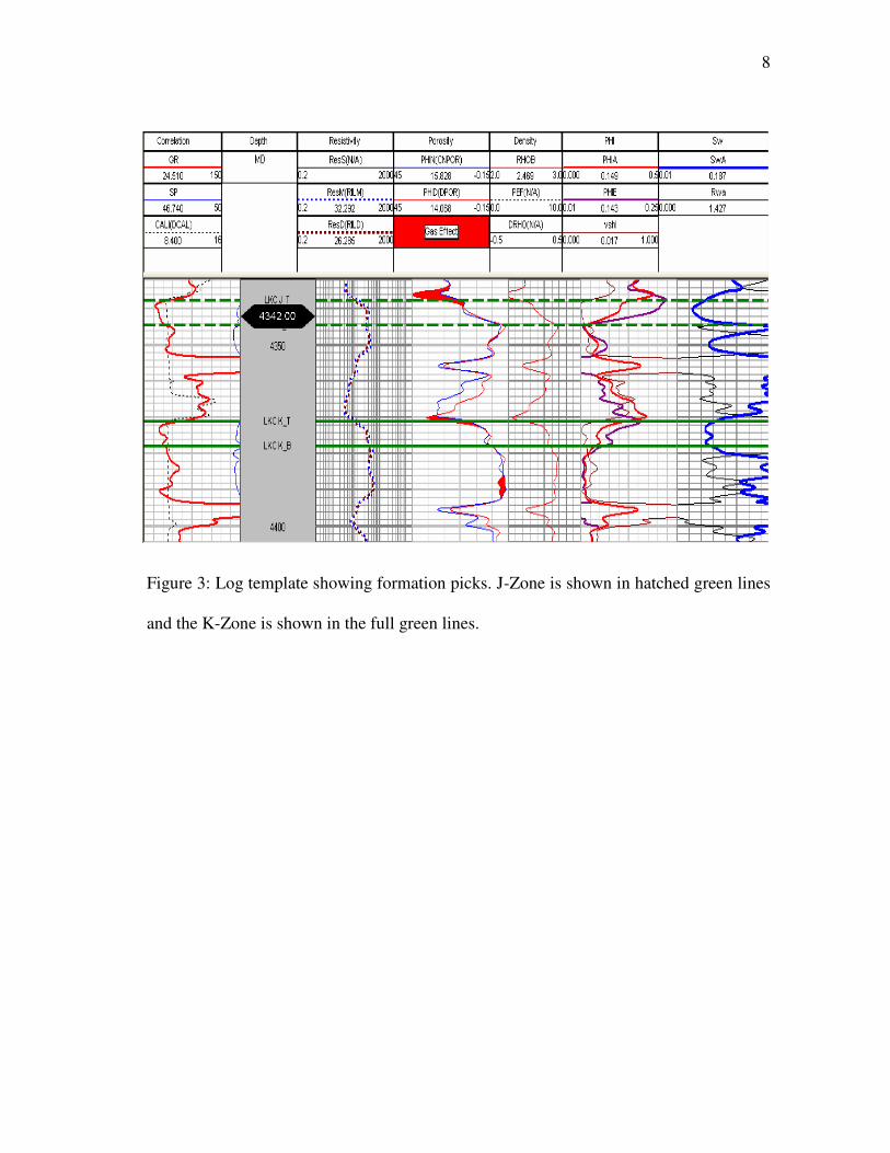
Following the general lithology identification in the flowchart is the picking of
formations (see Figure 3) and cross-sectional analysis. These are marked on from the
logs by getting information from drilling reports and verified by signatures on the
gamma ray logs and the caliper log which showed a slight size reduction due to
mudcake. Facies sequencing from gamma ray logs alone are very insignificant as
compared to a sandstone formation8. A stratigraphic and structural column of a cross-
section is made to help explain geologic and depositional trends of the environment.
This field is in a low-energy terrestrial environment with Phanerozoic sedimentary
rocks. These environments are dominated by mud-rich facies, where much of the
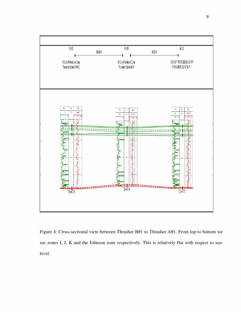
porosity is diagenetic in nature. The cross-section selected is an increasing path from
well to well across the field taken in a diagonal from Thrasher B#1 to Anderson C#1.
We observe a gently sloping depositional environment usually associated with lacustrine
deposits9. The cross-sections are analyzed in two segments shown in Figures 4 and 5.
8
Figure 3: Log template showing formation picks. J-Zone is shown in hatched green lines
and the K-Zone is shown in the full green lines.
9
Figure 4: Cross-sectional view between Thrasher B#1 to Thrasher A#1. From top to bottom we
see zones I, J, K and the Johnson zone respectively. This is relatively flat with respect to sea-
level.

10
Figure 5: Cross-sectional view between Thrasher A#1 to Anderson C#1. From top to
bottom we see zones I, J, K and the Johnson zone respectively
The typical Archie interpretation is used for the petrophysical analysis. This will
basically quantify porosity, net pay thickness and water saturation for identified zones.
The effect of shaliness on measured readings needs to be corrected before using log data
for analysis3. This is done by quantifying the shale volume. Shale volume was evaluated

11
using the gamma ray index and the steiber shale correction factor. This was used because
it is more conservative and goes well with younger rocks. The gamma ray index and the
Steiber equations are given as equations 1 and 2 respectively:
)(
)(,0(,1(
ln
ln_
cshl
c
GRshGRGR
GRGRMaxMinV
−
−= (1)
GRsh
GRsh
STshV
VV
_
_
_*23 −
= (2)
Gamma ray values of 20 API and 120 API were used for GRcln and GRshl
respectively. The shale volume calculation is used as a correction for the actual log
measurements as well as gives us a general trend of the vertical lithology distribution.
Porosity was determined from log measurments of neutron and density porosities. A
preferential average for porosity was evaluated as:
2
PHIDPHINPHIA
+= For PHIN ≤ 0.2 (3)
5
*2*3 PHINPHIDPHIA
+= For PHIN >0.2 (4)
This was corrected for shaliness by

12
)*( _ STshsh VPHIAPHIAPHIE −= (5)
The evaluation of water saturation by any means needs the proper evaluation of
the formation water resistivity5. The formation water resistivity was determined by two
methods. The apparent resistivity method and the pickett plot method was used. These
two methods were used since they utilize different data resources to an extent. The
formation resistivity was determined to be 0.06 ohm-meter. The Archie equation for
determining water saturation is given in Equation 6 as3:
n
t
m
w
wR
RaS
1
*
=
φ (6)
The Archie parameters a, m and n were obtained from the pickett plot by
estimating one parameter and the other two parameters are obtained. Given no core data,
it is safe to assume the saturation exponent as 2 which is the value used in most
reservoirs. Table 1 shows values obtained from Pickett plot analysis.
Table 1: Archie parameters.
Archie Parameter Value
a 1
m 1.6
n 2
13
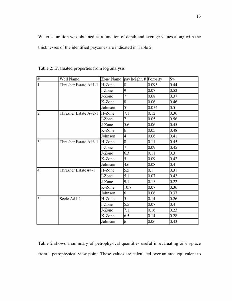
Water saturation was obtained as a function of depth and average values along with the
thicknesses of the identified payzones are indicated in Table 2.
Table 2: Evaluated properties from log analysis
# Well Name Zone Name pay height, ft Porosity Sw
H-Zone 8 0.095 0.44
I-Zone 9 0.07 0.52
J-Zone 7 0.08 0.37
K-Zone 8 0.06 0.46
Johnson 5 0.054 0.5
H-Zone 7.1 0.12 0.36
I-Zone 7 0.05 0.56
J-Zone 5.6 0.06 0.45
K-Zone 6 0.05 0.48
Johnson 4 0.06 0.41
H-Zone 8 0.11 0.45
I-Zone 7 0.09 0.45
J-Zone 6.3 0.11 0.3
K-Zone 5 0.09 0.42
Johnson 4.6 0.08 0.4
H-Zone 5.5 0.1 0.31
I-Zone 5.1 0.07 0.43
J-Zone 9.1 0.15 0.22
K-Zone 10.7 0.07 0.36
Johnson 6 0.06 0.37
H-Zone 5 0.14 0.26
I-Zone 5.5 0.07 0.4
J-Zone 7.1 0.16 0.23
K-Zone 6.5 0.14 0.28
Johnson 6 0.06 0.43
5 Seele A#1-1
4 Thrasher Estate #4-1
2 Thrasher Estate A#2-1
3 Thrasher Estate A#3-1
1 Thrasher Estate A#1-1
Table 2 shows a summary of petrophysical quantities useful in evaluating oil-in-place
from a petrophysical view point. These values are calculated over an area equivalent to

14
an area analysed by a geologist and the computed reserves compared. The compared
values are not equal but of the same order. The values in Table 2 are computed as an
average for the well from values in all layers.
15
CHAPTER III
DRILL STEM TESTING
Drill stem testing is conducted during the drilling phases of the well. This is the
pressure and flow evaluation of an indicated pay zone. An indicated pay zone is a zone
determined by a well site geologist either from a previous geophysical evaluation or
from drilling mud shows to be a potential zone of hydrocarbon accumulation. A good
drill stem test yields a sample of the type of reservoir fluid present, an indication of flow
rates, a measurement of the static and flowing bottom-hole pressure, an estimate of near-
wellbore formation permeability, skin factor and static reservoir pressure10.
Drill stem tests are pulsed tests10. These are pulsed in the sense that flow to the
surface is usually not appropriate since completion and production equipment is not yet
installed but the total fluid volumes must be known to evaluate the drill stem test
properly.
The test starts by opening the bottom-hole valve of the drill stem test equipment
allowing formation fluids to enter into the drill string. The first flow period is usually
short and is seen as a reservoir clean up10. The well is then shut-in and then opened again
for a second time for a longer period and then finally shut-in. During the flow and shut-
in periods, the drill stem test equipment measures the bottom-hole pressure and fluid
withdrawal at the surface is measured for volumetric calculation.
Analysis of drill stem data was done very carefully with a software application
that analyses the first and second build up using rigorous welltest techniques. The flow

16
segments are usually not analyzed with respect to pressure for two reasons being that the
rates are usually not known, and also the pressure recorded by the DST equipment
usually builds (particularly in oil reservoirs) with flow due to an increasing hydrostatic
column while a normal drawdown analysis goes with a pressure drop11.
Ideally, pressures from the two build-up phases are analyzed and extrapolated to
obtain extrapolated pressure and initial reservoir pressure. The flow segment is analyzed
to deduce rate information used in build-up test analysis. For this project, an average rate
is used as a constant rate. From an analysis of the first and second build-up, reservoir
depletion can be detected if extrapolated pressures from the two test segments do not
correspond and the pressure has completed building up in both segments. This was not
observed in the drill stem tests analyzed which meant at the field had potential at the
time of completion of the wells. The importance of a drill stem test can be summarized
by the following points:
• Evaluation of pressure, permeability and skin of an indicated pay interval.
• Evaluation of reservoir fluids in an indicated pay interval.
• Determination of completion details for an indicated pay interval.
• Evaluation of reservoir characterization (natural fractures)12.
From the mathematical theory behind the test, the well known diffusivity equation
in radial coordinates and dimensionless variables assuming a constant rate at the well
can be expressed as10:
17
D
D
D
D
DD
D
t
p
r
p
rr
p
∂
∂=
∂
∂+
∂
∂ 12
2
(7)
0)0,( =DD rp (8)
0),(lim =∞→
DDDr
trpD
(9)
1)0( =+wDp (10)
Equations 8-10 are boundary conditions. The wellbore pressure and the reservoir
pressure are coupled by the the Van Everdingen and Hurst skin effect10 as
1]),([)( =∂
∂−=
Dr
D
D
DDDDDwDr
psrtrptp (11)
Correa and Ramey used these equations to express the DST problem by
introducing a piecewise unit step function for the wellbore storage. The wellbore storage
coefficient for the production phase, CfD is defined as the volume of fluid accumulated in
the wellbore per unit change in wellbore pressure. Essentially, the relationship is given
as
0 , 0][])1[( 1 >=∂
∂−+− = Dr
D
D
D
D
wD
sDtfDt tr
pr
dt
dpCHCH
D (12)

18
where Ht is a unit-step function and CsD is the static wellbore storage. The main
difference between CfD and CsD is the relationship between the fluid compressibility and
pressure. For slightly compressible fluids (oil) these are approximately the same values.
Equation 12 is solved using laplace transforms and appropriate boundary conditions,
Correa and Ramey obtained the solution as:
∫ −−+=t
DDwDDDsDDfDsDDsDDsDDwD dptCsPCCtCsPCtp0
)('),,()(),,()( τττ (13)
Equation 13 holds the fact that as the flow time goes to zero, the integral term
vanishes and the result converges to the “slug test” solution used in groundwater
analysis. This poses a practical issue that the flow periods should be kept to a minimum
with respect to the shut-in times for a proper DST analysis.
Equation 13 can be represented in dimensional form as
tt
tmptp
p
p
ciw∆+
−=)( (14)
Where the slope mc is defined as
−+=
p
wfis
cqt
ppC
kh
qm
)(1
4π
µ (15)
19
and is representative of the flow regime of the pressure transient. The skin effect is
calculated from
][log5.02
fD
s
D
eC
eCs = (16)
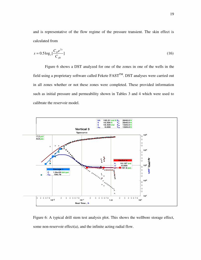
Figure 6 shows a DST analyzed for one of the zones in one of the wells in the
field using a proprietary software called Fekete FASTTM. DST analyses were carried out
in all zones whether or not these zones were completed. These provided information
such as initial pressure and permeability shown in Tables 3 and 4 which were used to
calibrate the reservoir model.
Figure 6: A typical drill stem test analysis plot. This shows the wellbore storage effect,
some non-reservoir effect(a), and the infinite acting radial flow.
10-2 10-1 1.0 1013 4 5 6 7 8 2 3 4 5 6 7 8 2 3 4 5 6 7 8 2 3 4 5 6 7 8
Real Time , h
101
102
103
104
105
2
3
5
8
2
3
5
8
2
3
5
7
2
3
5
8
∆∆ ∆∆p (P
PD
) , psi/h
Typecurv e
Vertical 3
1167.2 psi1166.8 psi
kh 193.51 md.fth 10.500 ftk 18.429 mdsd 0.000
Xe 2640.0 ftYe 2640.0 ftXw 1320.0 ftYw 1320.0 ft
Radial 0
k 18.197 mds' -0.069p* 1167.6 psi
Storage 1
C 1.8e-04 bbl/psiCD 196.79

20
Table 3: DST results of 6 wells analyzed using commercial software. Results follow
irregular trends as suggested by geological history.
Zone Name Pressure, psi Permeability, md Skin
H 1285 181.5 0
I 1335 1479 0.6
J 1370 258.9 2.5
K 1265 8.7 2.9
Johnson 412 5.8 -2.5
H 1290 26.1 -2.2
I 727 74.5 14
J 812 178 2.4
K 1226 15 -1.5
Johnson 506 53 -3.4
H 745 4.5 -1
I 683 33 18.3
J DST fault N/A N/A
K 1113 5.3 0.5
Johnson 423 7.8 -1.5
H 1228 17.1 -0.6
I 278 258.4 4.2
J 350 180 2.2
K 1022 17.8 -3
Johnson 520 94.5 -2
H 906 160 0
I 291 124 7
J 331 165 0
K 1146 10.6 1.6
Johnson 1130 9 -1.3
H 947 112 1.4
I 402 6.5 5.2
J 300 360 2.8
K 1145 87 3
Johnson 1050 46 -1.9
Thrasher B#1 2/12/2003
Thrasher A#4 1/6/2003
Seele A#1 2/11/2003
Thrasher A#3 10/4/2002
Thrasher A#2 10/7/2002
Zonal DST AnalysisWell Name Date Completed
4/11/2002Thrasher A#1
21
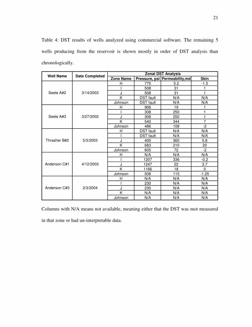
Table 4: DST results of wells analyzed using commercial software. The remaining 5
wells producing from the reservoir is shown mostly in order of DST analysis than
chronologically.
Zone Name Pressure, psi Permeability,md Skin
H 775 5.2 -1.5
I 508 31 1
J 508 31 1
K DST fault N/A N/A
Johnson DST fault N/A N/A
H 906 19 1
I 308 250 1
J 308 250 1
K 540 344 7
Johnson 486 108 -2
H DST fault N/A N/A
I DST fault N/A N/A
J 400 365 0.8
K 683 210 20
Johnson 605 72 -2
H N/A N/A N/A
I 1207 336 -0.2
J 1247 22 3.7
K 1166 18 0
Johnson 508 115 -1.25
H N/A N/A N/A
I 230 N/A N/A
J 230 N/A N/A
K N/A N/A N/A
Johnson N/A N/A N/A
Thrasher B#2
2/3/2004Anderson C#3
5/3/2003
Anderson C#1 4/12/2003
Zonal DST Analysis
Seele A#2 3/14/2003
Seele A#3 3/27/2002
Well Name Date Completed
Columns with N/A means not available, meaning either that the DST was mot measured
in that zone or had un-interpretable data.
22
CHAPTER IV
RESERVOIR MODEL DEVELOPMENT
A reservoir simulation model is a mathematical (mostly numerical)
representation of a petroleum reservoir6. A simulation model is built to represent an oil
and gas reservoir in its size, shape and physical characteristics. The physical
characteristics usually represented include but is not limited to pressure, fluid
saturations, reservoir porosity, permeability, relative permeability, and influence
functions.
Data gathering usually precedes reservoir model construction. Data gathered
from different sources must be coherent before being incorporated into a model6. This
helps the modeling process to be direct as it is usually the case in deterministic
modeling. In achieving a good reservoir model we applied strict reservoir engineering
sense while honoring geology and preserving petrophysical analysis. Following the
reservoir model development is the validation which is principally done by a well known
tool called history matching.
Deterministic Modeling
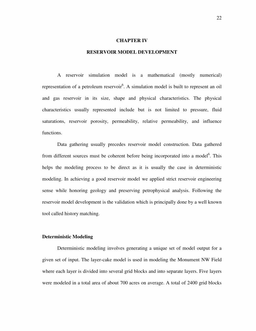
Deterministic modeling involves generating a unique set of model output for a
given set of input. The layer-cake model is used in modeling the Monument NW Field
where each layer is divided into several grid blocks and into separate layers. Five layers
were modeled in a total area of about 700 acres on average. A total of 2400 grid blocks
23
were used to model the anticlinal reservoir structure. These gridblocks were now
populated with values from well control values which was obtained from well logs and
drill stem test. Using the fact that we have lateral and vertical heterogeneity some typical
methods are used in populating the porosity and permeability values13. Also worth
mentioning is the relative permeability tables which was developed using work from
Byrnes and Bhattercharyna and drill stem tests.
Porosity Description
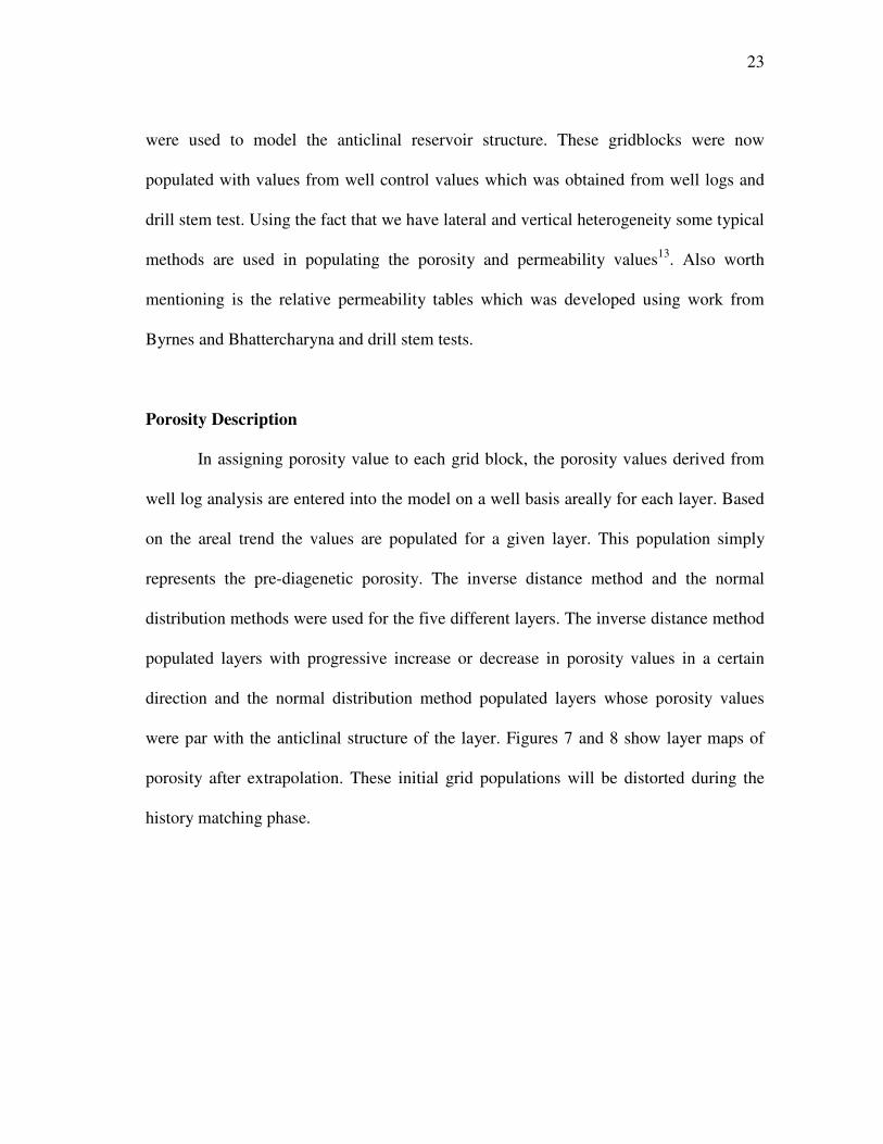
In assigning porosity value to each grid block, the porosity values derived from
well log analysis are entered into the model on a well basis areally for each layer. Based
on the areal trend the values are populated for a given layer. This population simply
represents the pre-diagenetic porosity. The inverse distance method and the normal
distribution methods were used for the five different layers. The inverse distance method
populated layers with progressive increase or decrease in porosity values in a certain
direction and the normal distribution method populated layers whose porosity values
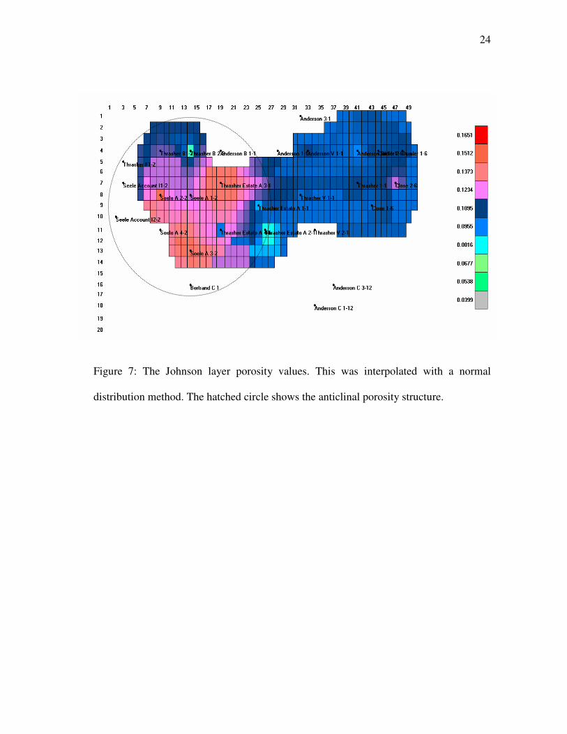
were par with the anticlinal structure of the layer. Figures 7 and 8 show layer maps of
porosity after extrapolation. These initial grid populations will be distorted during the
history matching phase.
24
Figure 7: The Johnson layer porosity values. This was interpolated with a normal
distribution method. The hatched circle shows the anticlinal porosity structure.
25
Figure 8: The H-Zone layer porosity values. This was interpolated with an inverse
distance method.
Permeability Description
The permeability values were principally obtained from drillstem test analysis for
each zone and this was populated using a logarithmic extrapolation. This method of
extrapolation accounts for heterogeneity by covering a wider range of values. However,
it must be noted that the derived extrapolated permeabilities are not final. These will be
calibrated during the history-matching process to obtain a good match.
26
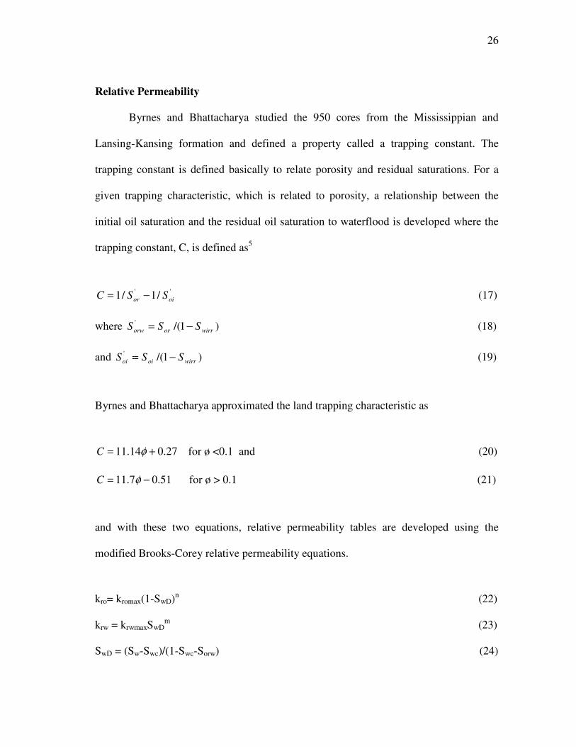
Relative Permeability
Byrnes and Bhattacharya studied the 950 cores from the Mississippian and
Lansing-Kansing formation and defined a property called a trapping constant. The
trapping constant is defined basically to relate porosity and residual saturations. For a
given trapping characteristic, which is related to porosity, a relationship between the
initial oil saturation and the residual oil saturation to waterflood is developed where the
trapping constant, C, is defined as5
'' /1/1 oior SSC −= (17)
where )1/('
wirrororw SSS −= (18)
and )1/('
wirroioi SSS −= (19)
Byrnes and Bhattacharya approximated the land trapping characteristic as
27.014.11 += φC for ø <0.1 and (20)
51.07.11 −= φC for ø > 0.1 (21)
and with these two equations, relative permeability tables are developed using the
modified Brooks-Corey relative permeability equations.
kro= kromax(1-SwD)n (22)
krw = krwmaxSwDm (23)
SwD = (Sw-Swc)/(1-Swc-Sorw) (24)

27
Two different relative permeability tables shown in Figures 9 and 10 were
defined for two rock types. These two relative permeability curves had different
propensity for water. The H-Zone and the K-Zone had a good propensity for water with
the H-Zone having an aquifer. The I, J and Johnson zone had predominantly the same
flow characteristics. The endpoints in equation 24 were satisfied iteratively from DST
analysis and from the land trapping characteristic. Fluids produced during the drill stem
test were analyzed to understand fluid flow characteristics for each zone. This was then
tied against the permeability derived from the drill stem test analysis which basically
give the permeability to oil.
Relative Permeability Table for Tight zones
0
0.1
0.2
0.3
0.4
0.5
0.6
0.7
0.8
0.9
1
0 0.1 0.2 0.3 0.4 0.5 0.6 0.7Sw
k-r
o
0
0.1
0.2
0.3
0.4
0.5
0.6
k-r
w
k-ro
k-rw
Relative Permeability Table for Vuggy zones
0
0.1
0.2
0.3
0.4
0.5
0.6
0.7
0.8
0.9
1
0 0.1 0.2 0.3 0.4 0.5 0.6 0.7
Sw
k-r
o
0
0.1
0.2
0.3
0.4
k-r
w
k-ro
k-rw
Figure 9: Relative permeability
table for tight zones. This has a
higher water propensity due to a
higher capillary pressure of the
non-wetting fluid.
Figure 10: Relative permeability
table for vuggy zones. This has a
lower water propensity due to a
lower capillary pressure of the non-
wetting fluid.

28
Capillary Pressure and Initial Water Saturation
Initial water saturation is usually determined from capillary pressure entered into
relative permeability tables14. This method creates a water distribution profile with
depth. For the Monument Northwest field, the average net pay was about 5 ft. This does
not leave room for a distribution profile without drastic changes. The initial water
saturation for layers other than the H-Zone are assumed to be at or close to irreducible
water saturation following geological history. To account for an initial water distribution
in the H-Zone, a spatial relationship was developed that varied the water saturations
laterally. The water saturation was distributed as a function of net pay height. This made
the water saturation least at the top of the structure which had the highest net pay and the
highest water saturation at the flanks were pinch-outs occur and aquifer starts. The H-
Zone water saturation was defined in this manner and this helped increase the water
production history match where the flank wells had higher water production. This ties in
with the fluid migration history where water-in-place would settle due to buoyancy and
migration direction. A linear relationship was developed as
)( max
minmax
max hhhh
SSSS wcw
wcw −−
−+= (25)

29
Aquifer Definition
A Carter-Tracy aquifer was modeled at the top of the structure (H-Zone). This
was done by influencing grid blocks on the west flank of the field. This aquifer is tied in
with the migration and accumulation of the hydrocarbons which displaced formation
water which was still trapped in the structure. The Carter-Tracy equation is given in
finite difference form as15
)(
))()((11
1110
1
++
+++
+
−
−−−=
n
t
n
D
n
t
n
D
n
D
n
t
n
e
n
n
e
n
e
DD
D
ptp
ttpWppFWW (26)
Where F is a constant and ptD is the pressure influence function at tD. For a finite aquifer
this is proportional to the natural logarithm of ra/rw. After defining the aquifer, we used a
horizontal influx function (using face x-z and y-z of west flank grid blocks) for aquifer
fluid displacement.
It should be noted that the aquifer modeled was not modeled in the initial model
development but during the history matching phase of the project. It is done this way to
know how to calibrate and model the aquifer as a finite aquifer by checking the pressure
offsets in the layer pressure match for the H-Zone. More so, other aquifer data such as
the aquifer permeability was calibrated by the water production match from the wells
producing in the H-Zone.
30
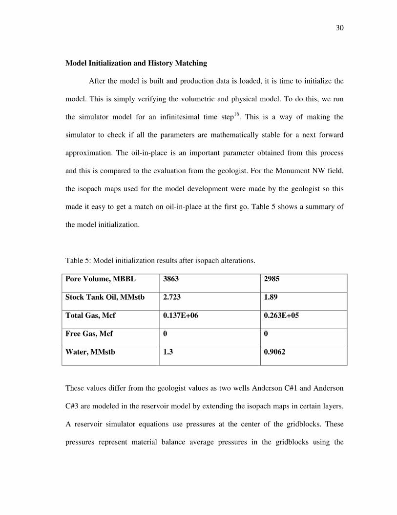
Model Initialization and History Matching
After the model is built and production data is loaded, it is time to initialize the
model. This is simply verifying the volumetric and physical model. To do this, we run
the simulator model for an infinitesimal time step16. This is a way of making the
simulator to check if all the parameters are mathematically stable for a next forward
approximation. The oil-in-place is an important parameter obtained from this process
and this is compared to the evaluation from the geologist. For the Monument NW field,
the isopach maps used for the model development were made by the geologist so this
made it easy to get a match on oil-in-place at the first go. Table 5 shows a summary of
the model initialization.
Table 5: Model initialization results after isopach alterations.
Pore Volume, MBBL 3863 2985
Stock Tank Oil, MMstb 2.723 1.89
Total Gas, Mcf 0.137E+06 0.263E+05
Free Gas, Mcf 0 0
Water, MMstb 1.3 0.9062
These values differ from the geologist values as two wells Anderson C#1 and Anderson
C#3 are modeled in the reservoir model by extending the isopach maps in certain layers.
A reservoir simulator equations use pressures at the center of the gridblocks. These
pressures represent material balance average pressures in the gridblocks using the

31
diffusivity equation as the flow condition for displacing the oil and gas under a finite
difference scheme. The diffusivity equation is simply a combination of the equation of
state, the continuity equation and conservation principle. This is simply given as17 (in
global space)
t
pp
∂
∂=∇ α2 (27)
and can be discretized in a one-dimensional cartesian coordinate as17
t
p -p
k 0.00633
c =
)x(
p +p2 -pn
i
1+n
i
2
1+n
1+i
1+n
i
1+n
1-i
∆∆
φµ (28)
For gridblocks holding wells, additional equations are used to relate well performance to
cell variables. Assuming steady state flow occurs within a cell, flow equations are given
as14:
)( 1
,mod wf
n
ji
n
o
r
elo ppB
kJq −
= +
µ (29)
)( 1
,mod wf
n
ji
n
w
relw pp
B
kJq −
= +
µ (30)
o
n
wf
n
ji
n
g
relg qRspp
B
kJq
11
,mod )( ++ +−
=
µ (31)
Where Jmodel is the well index given by Peaceman as17

32
srr
khJ
wo
el+
=/ln
)00633.0(2mod
π (32)
And ro is calculated based on permeability anisotropy. Equations 29-31 present
three equations with four unknowns: qo, qw, qg and pwf. This implies that for a simulator
run, the user must specify one of these unknowns and the simulator will produce the
well17. After the well is produced, we can compare simulator performance with actual
data if available. This is a vital step in simulation as this helps to reduce uncertainty of
the simulator model. This is called reservoir history matching.
History-matching is the process of calibrating the reservoir model so that the
simulator results closely follows or is the same as the observed data. Production data and
pressure are measurements used during this phase. Typically for a reservoir simulator
run, either the fluid rate is specified or a pressure constraint is used to satisfy the material
balance16.
We used the fluid withdrawal constraint for this project. This scheme uses
production data which was measured and recorded as a simulator input. The fluid was
then withdrawn, and a pressure match was obtained. A total of 11 wells and 5 zones
would be matched. To do this, we constructed a flow diagram that assisted us in the
history matching process. This was done in a chronological manner by well completion
time history following a zone-zone basis. After covering a reasonable acreage, the match
is continued on a proximity basis. The chart shown in Figure 11 gives an idea on how to
calibrate reservoir properties for obtaining a match with less iteration.

33
Figure 11: Chronological chart of the first seven completed wells. Different colors of
arrow represent different zones, and going into a well represents a completion of the well
in that zone.
Thrasher A#1
Thrasher A#3
Thrasher A#2
Thrasher A#4
Seele A#1
Thrasher B#1
Seele A#2
Thrasher A#1
Thrasher A#3
Thrasher A#2
Thrasher A#4
Seele A#1
Thrasher B#1
Seele A#2
34
Pressure History for Thrasher A#1 Layers
0
200
400
600
800
1000
1200
1400
1600
0 500 1000 1500 2000 2500 3000 3500
Time, days
Pre
ss
ure
, p
si
H-Zone Sim BHP
I-Zone Sim BHP
J-Zone Sim BHP
K-Zone Sim BHP
Johnson Zone Sim BHP
H-Zone Hist BHP
I-Zone Hist BHP
K-Zone Hist BHP
Johnson Zone Hist BHP
J-Zone Hist BHP
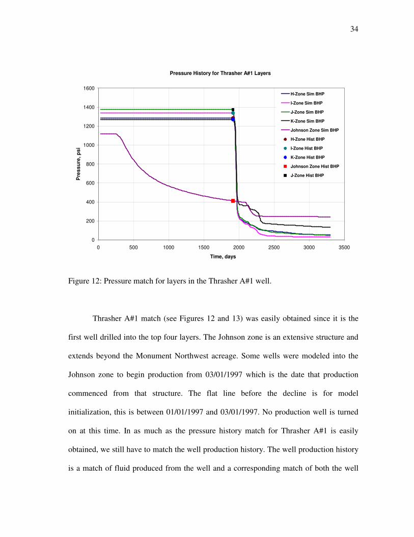
Figure 12: Pressure match for layers in the Thrasher A#1 well.
Thrasher A#1 match (see Figures 12 and 13) was easily obtained since it is the
first well drilled into the top four layers. The Johnson zone is an extensive structure and
extends beyond the Monument Northwest acreage. Some wells were modeled into the
Johnson zone to begin production from 03/01/1997 which is the date that production
commenced from that structure. The flat line before the decline is for model
initialization, this is between 01/01/1997 and 03/01/1997. No production well is turned
on at this time. In as much as the pressure history match for Thrasher A#1 is easily
obtained, we still have to match the well production history. The well production history
is a match of fluid produced from the well and a corresponding match of both the well

35
historical static bottom-hole pressure and the flowing bottom hole pressure. The
Thrasher A#1 well was put on a pumping unit within months of production, therefore we
expect to see a minimal flowing bottom hole pressure as shown below:
Well Historical Plot for Thrasher A#1
0
200
400
600
800
1000
1200
1400
0 500 1000 1500 2000 2500 3000 3500
Time, Days
Pre
ss
ure
, p
si
0
50
100
150
200
250
Ra
te,
bb
l/d
Flowing BHP
Reservoir BHP
Sim Oil Production Rate
Hist Oil Production Rate
Figure 13: Well historical plot for Thrasher A#1. This shows the bottom-hole pressure
reducing with production and the well pumped off.
The layer pressure match is first obtained for all wells before a single well
production history match is made. This was achieved by specifying a total reservoir fluid
volume (oil and water) constraint to first match the layer pressures. This ensured that the
fluid actually produced from the reservoir can actually be matched. The constraint was

36
then reverted back to an oil-rate constraint for which a well production history match
was made followed finally by a fluid match on a well basis. This is shown with a flow
chart in Figure 14:
Figure 14: Flow diagram for history matching process used. Decision 2 usually throws
off automatic history matching schemes.
q, k, φ, Aq, s, kr, Swq, k, φ, Aq, s, kr, Sw
Well fluid match?
Pressure match?
Well history
match?
kr, kaq, Sw
k, q, sY
N
N
Y
N
qt
qo
k, Aq, φ
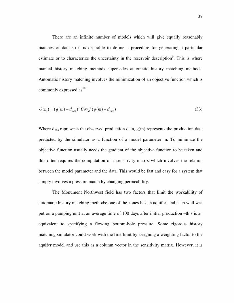
37
There are an infinite number of models which will give equally reasonably
matches of data so it is desirable to define a procedure for generating a particular
estimate or to characterize the uncertainty in the reservoir description6. This is where
manual history matching methods supersedes automatic history matching methods.
Automatic history matching involves the minimization of an objective function which is
commonly expressed as18
))(())(()( 1
obsd
T
obs dmgCovdmgmO −−= − (33)
Where dobs represents the observed production data, g(m) represents the production data
predicted by the simulator as a function of a model parameter m. To minimize the
objective function usually needs the gradient of the objective function to be taken and
this often requires the computation of a sensitivity matrix which involves the relation
between the model parameter and the data. This would be fast and easy for a system that
simply involves a pressure match by changing permeability.
The Monument Northwest field has two factors that limit the workability of
automatic history matching methods: one of the zones has an aquifer, and each well was
put on a pumping unit at an average time of 100 days after initial production –this is an
equivalent to specifying a flowing bottom-hole pressure. Some rigorous history
matching simulator could work with the first limit by assigning a weighting factor to the
aquifer model and use this as a column vector in the sensitivity matrix. However, it is

38
virtually impossible to work automatically with the second constraint. This would imply
imposing a double standard on the simulator.
Inasmuch as the second constraint is ambiguous, it helps improve our model with
respect to the history matching process. Actually, this was one of the biggest advantages
of manual history matching methods with respect to this project. The reservoir engineer
now knows every corner of the reservoir and a better knowledge and reservoir
characterization of the reservoir is achieved. For example, after tweaking permeability
within a reasonable range and a well production history match is not achievable in the
simulator, we can infer that the actual well must be damaged and that was why it
required a pumping unit early in the life of a well. So to achieve the historical event of
the pumping unit, we now add a skin to the well which now facilitates the excessive
pressure drop at the well. Such well would be tagged as a stimulation candidate
particularly if the production rate drops from a usual trend.
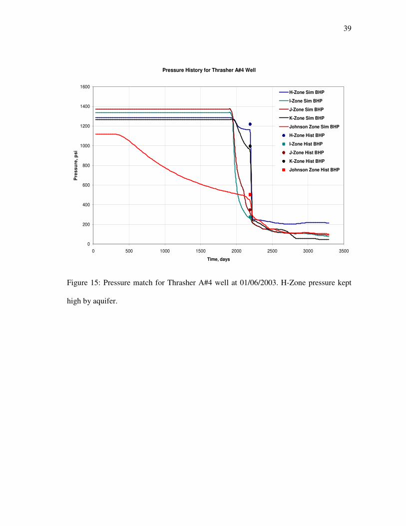
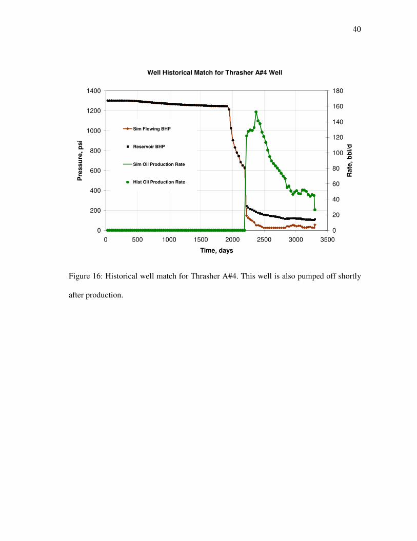
Figures 15-17 show the match for Thrasher A#4 well which went under
production 8 months after Thrasher A#1:
39
Pressure History for Thrasher A#4 Well
0
200
400
600
800
1000
1200
1400
1600
0 500 1000 1500 2000 2500 3000 3500
Time, days
Pre
ss
ure
, p
si
H-Zone Sim BHP
I-Zone Sim BHP
J-Zone Sim BHP
K-Zone Sim BHP
Johnson Zone Sim BHP
H-Zone Hist BHP
I-Zone Hist BHP
J-Zone Hist BHP
K-Zone Hist BHP
Johnson Zone Hist BHP
Figure 15: Pressure match for Thrasher A#4 well at 01/06/2003. H-Zone pressure kept
high by aquifer.
40
Well Historical Match for Thrasher A#4 Well
0
200
400
600
800
1000
1200
1400
0 500 1000 1500 2000 2500 3000 3500
Time, days
Pre
ss
ure
, p
si
0
20
40
60
80
100
120
140
160
180
Ra
te,
bb
l/d
Sim Flowing BHP
Reservoir BHP
Sim Oil Production Rate
Hist Oil Production Rate
Figure 16: Historical well match for Thrasher A#4. This well is also pumped off shortly
after production.
41
Fluid Match for Thrasher A#4 Well
0
20
40
60
80
100
120
140
160
180
0 500 1000 1500 2000 2500 3000 3500
Time, days
Oil
Pro
du
cti
on
Ra
te,
bb
l/d
0
2
4
6
8
10
12
Wate
r P
rod
uc
tio
n R
ate
, b
bl/d
Sim Oil Production
Hist Oil Production
Sim Water Production
Hist Water Production
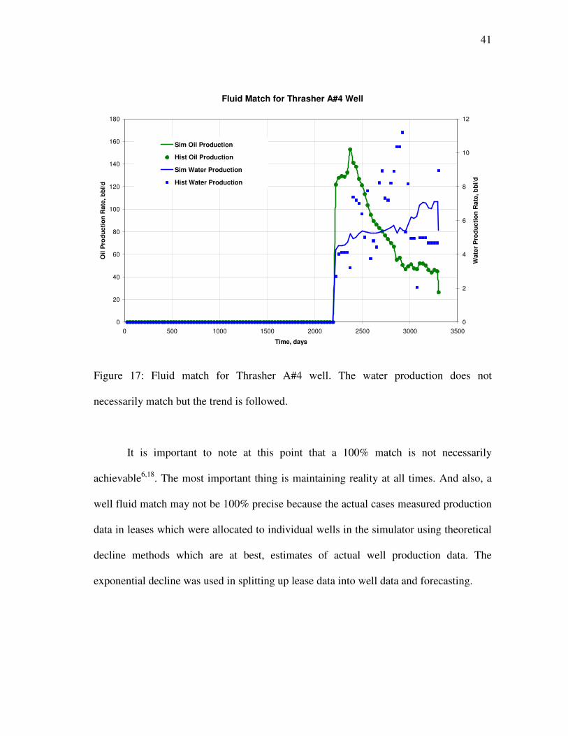
Figure 17: Fluid match for Thrasher A#4 well. The water production does not
necessarily match but the trend is followed.
It is important to note at this point that a 100% match is not necessarily
achievable6,18. The most important thing is maintaining reality at all times. And also, a
well fluid match may not be 100% precise because the actual cases measured production
data in leases which were allocated to individual wells in the simulator using theoretical
decline methods which are at best, estimates of actual well production data. The
exponential decline was used in splitting up lease data into well data and forecasting.
42
CHAPTER V
WATERFLOODING MONUMENT NW FIELD
Simulating a waterflood was the objective of the overall study. Now that we have a
replica of the reservoir we simulate a waterflood recovery by injection. A few factors
should be considered and analyzed before a waterflood19. For the Monument Northwest
field these included:
• Selection of injection wells
• Fracture gradient of the formation
• Proposed injection rate and cumulative injection volume for a full sweep
• Conversion costs of well
• Gravitational and discretization effects
Layer Subdivision
Before discussing the details of the waterflood, it is important to explain the
discretization and gravitational effects of a water injection with respect to the
displacement in the grid block. When there is an influx of saturation on a grid block, the
simulator implicitly satisfies material balance for that grid block by displacing inherent
saturations and increasing the grid block pressure. The simulator also tries to satisfy the
gravitational effects of the different saturations. This can lead to numerical dispersion
which is a common problem with simulators. Numerical dispersion simply means a
blow-up of discretization errors. We helped minimize this problem in this project using
43
layer subdivision prior to injection. We simply divided a layer into three equal
compartments with same properties. The idea behind this is that if you inject into H-
Zone, which is now in three layers, water will preferentially fill the lowest layer. This
helped reduce the dispersion problems while at the same time simulating reality.
Selection of Injection Wells
This was not a simple straight-forward task as this involved zones that are all of
different area, shape and with different number of wells. As usual, we tried using our
constraints as leverages in our analysis. Using the constraints, we tried optimizing areal
sweep efficiency and minimizing water breakthrough time for producer wells while
checking that actual injection rates can be achieved with the stated fracture gradient
bearing in mind that the areal sweep efficiency of a waterflood before breakthrough is
directly proportional to the recovery19.
The injection rate is proportional to the injection pressure and the injection
pressure should be less than the fracture pressure hence a fracture would occur19,20. The
fracture pressure is simply the fracture gradient multiplied by the corresponding depth.
Therefore to achieve good injection rates without back-pressure or fracturing, the
reservoir permeability should be favorable. The injection rate and injection pressure are
given by Darcy’s law as10,19
)/ln(
)(00708.0__
weo
wft
wrr
pphki
µ
−= (34)
44
where _
k is the average combined layer permeability calculated as
th
hkhkhkhkhkk 5544332211_ ++++
= (35)
From equation 34, we observe that to inject below the fracture pressure, the
reservoir pressure and the permeability play the most important. From the fact that we
have lateral heterogeneity in the reservoir, we used the radial permeability of the grid
block holding the well for the computation of equation 35. This assumes that the grid
blocks holding the well transmits the water and should a fracture occur, it should start
from the well20,21. A field injection rate constraint of 1000 bbl/d was used together with a
maximum injection pressure of 2500 psi for each well. This maximum injection pressure
was justified using a fracture gradient of 0.7 psi/ft with a safety gradient of 0.1 psi/ft.
This upper limit watched the window because to inject at the constant injection rate, the
injection pressure will increase due to increased reservoir pressure. Therefore there
comes a time when the injection rate may be reduced to satisfy the maximum injection
pressure constraint or the simulator will quit in error. This is observed from the
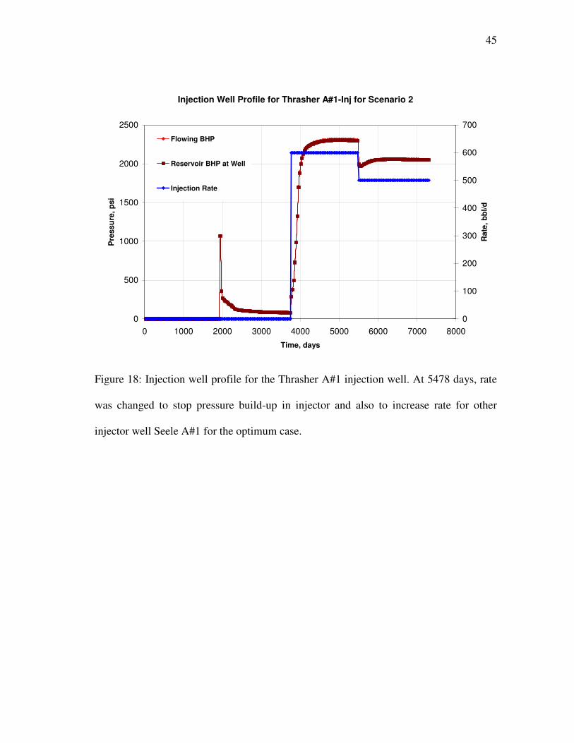
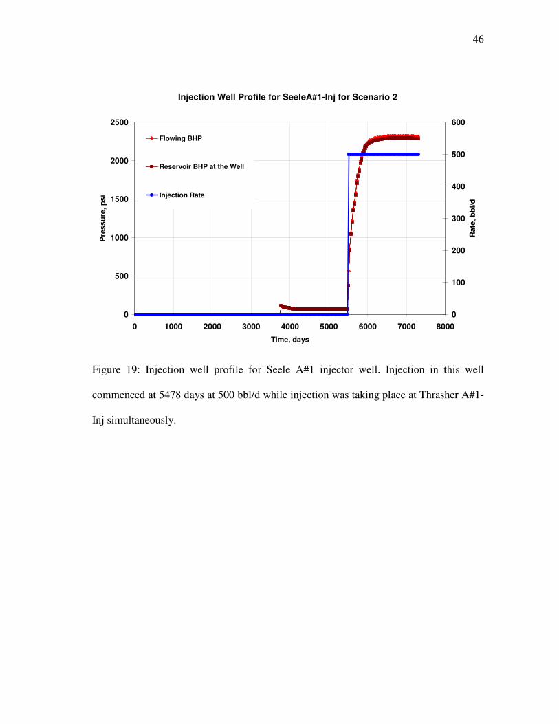
simulated injection wells’ profile (see Figures 18 and 19) where the flowing bottomhole
pressure and the injection rate for the injector well is plotted together against time.
45
Injection Well Profile for Thrasher A#1-Inj for Scenario 2
0
500
1000
1500
2000
2500
0 1000 2000 3000 4000 5000 6000 7000 8000
Time, days
Pre
ss
ure
, p
si
0
100
200
300
400
500
600
700
Ra
te,
bb
l/d
Flowing BHP
Reservoir BHP at Well
Injection Rate
Figure 18: Injection well profile for the Thrasher A#1 injection well. At 5478 days, rate
was changed to stop pressure build-up in injector and also to increase rate for other
injector well Seele A#1 for the optimum case.
46
Injection Well Profile for SeeleA#1-Inj for Scenario 2
0
500
1000
1500
2000
2500
0 1000 2000 3000 4000 5000 6000 7000 8000
Time, days
Pre
ss
ure
, p
si
0
100
200
300
400
500
600
Rate
, b
bl/
d
Flowing BHP
Reservoir BHP at the Well
Injection Rate
Figure 19: Injection well profile for Seele A#1 injector well. Injection in this well
commenced at 5478 days at 500 bbl/d while injection was taking place at Thrasher A#1-
Inj simultaneously.
47
Waterflood Scenarios
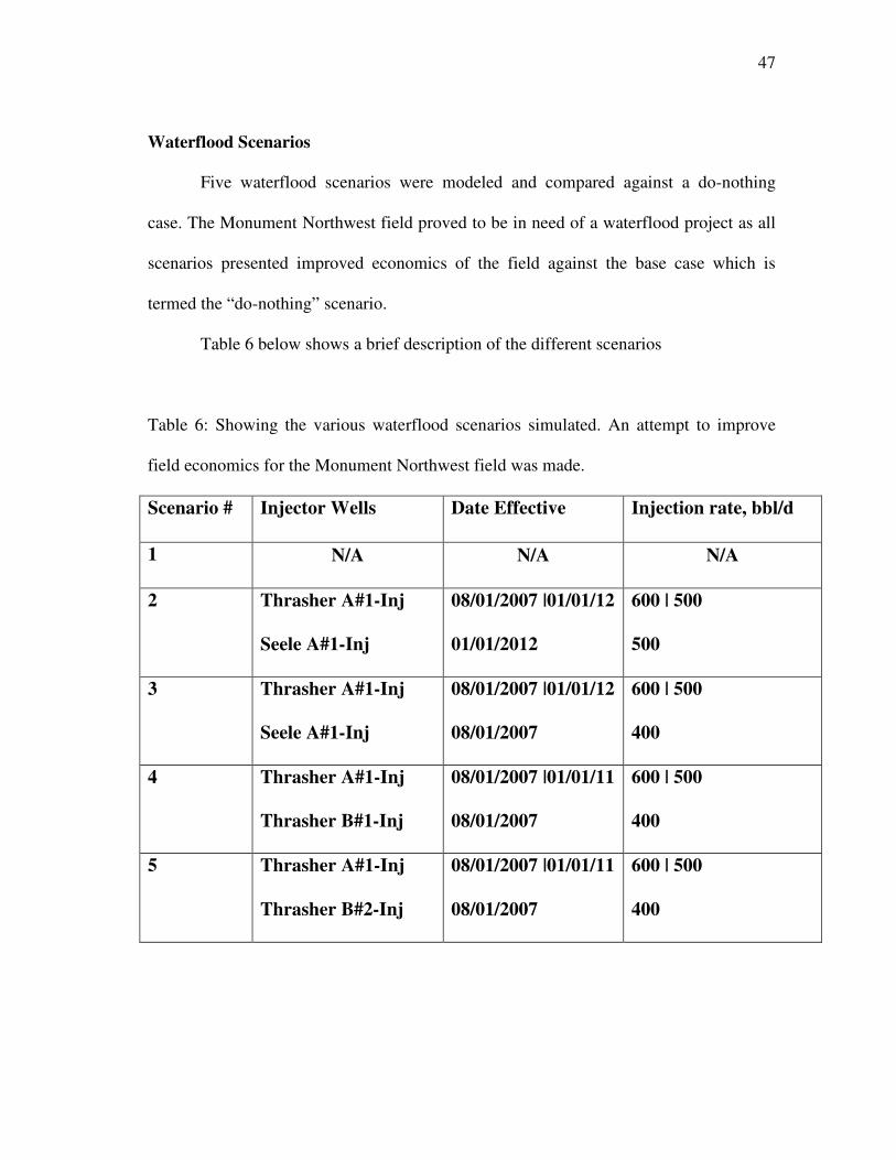
Five waterflood scenarios were modeled and compared against a do-nothing
case. The Monument Northwest field proved to be in need of a waterflood project as all
scenarios presented improved economics of the field against the base case which is
termed the “do-nothing” scenario.
Table 6 below shows a brief description of the different scenarios
Table 6: Showing the various waterflood scenarios simulated. An attempt to improve
field economics for the Monument Northwest field was made.
Scenario # Injector Wells Date Effective Injection rate, bbl/d
1 N/A N/A N/A
2 Thrasher A#1-Inj
Seele A#1-Inj
08/01/2007 |01/01/12
01/01/2012
600 | 500
500
3 Thrasher A#1-Inj
Seele A#1-Inj
08/01/2007 |01/01/12
08/01/2007
600 | 500
400
4 Thrasher A#1-Inj
Thrasher B#1-Inj
08/01/2007 |01/01/11
08/01/2007
600 | 500
400
5 Thrasher A#1-Inj
Thrasher B#2-Inj
08/01/2007 |01/01/11
08/01/2007
600 | 500
400
48
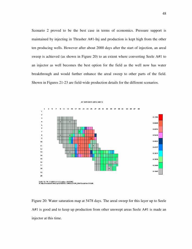
Scenario 2 proved to be the best case in terms of economics. Pressure support is
maintained by injecting in Thrasher A#1-Inj and production is kept high from the other
ten producing wells. However after about 2000 days after the start of injection, an areal
sweep is achieved (as shown in Figure 20) to an extent where converting Seele A#1 to
an injector as well becomes the best option for the field as the well now has water
breakthrough and would further enhance the areal sweep to other parts of the field.
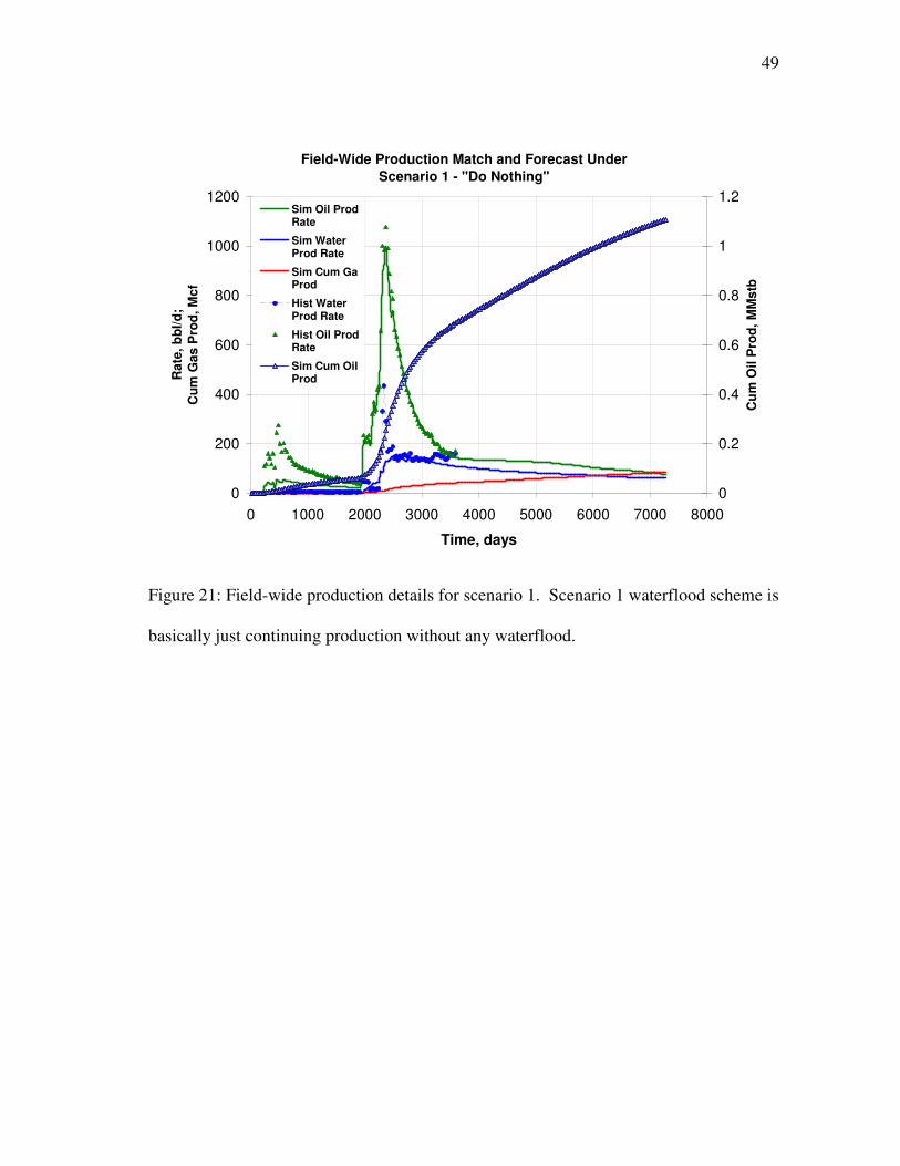
Shown in Figures 21-23 are field-wide production details for the different scenarios.
Figure 20: Water saturation map at 5478 days. The areal sweep for this layer up to Seele
A#1 is good and to keep up production from other unswept areas Seele A#1 is made an
injector at this time.
49
Field-Wide Production Match and Forecast Under
Scenario 1 - "Do Nothing"
0
200
400
600
800
1000
1200
0 1000 2000 3000 4000 5000 6000 7000 8000
Time, days
Ra
te,
bb
l/d
;
Cu
m G
as
Pro
d,
Mcf
0
0.2
0.4
0.6
0.8
1
1.2
Cu
m O
il P
rod
, M
Ms
tb
Sim Oil ProdRate
Sim WaterProd Rate
Sim Cum GaProd
Hist WaterProd Rate
Hist Oil ProdRate
Sim Cum OilProd
Figure 21: Field-wide production details for scenario 1. Scenario 1 waterflood scheme is
basically just continuing production without any waterflood.
50
Field-Wide Production Match and Forecast Under
Scenario 2
0
200
400
600
800
1000
1200
0 1000 2000 3000 4000 5000 6000 7000 8000
Time, days
Ra
te,
bb
l/d
;
Cu
m G
as
Pro
d,
Mcf
0
0.2
0.4
0.6
0.8
1
1.2
Cu
m O
il P
rod
, M
Ms
tb
Sim Oil ProdRate
Sim WaterProd Rate
Sim Cum GaProd
Hist WaterProd Rate
Hist Oil ProdRate
Sim Cum OilProd
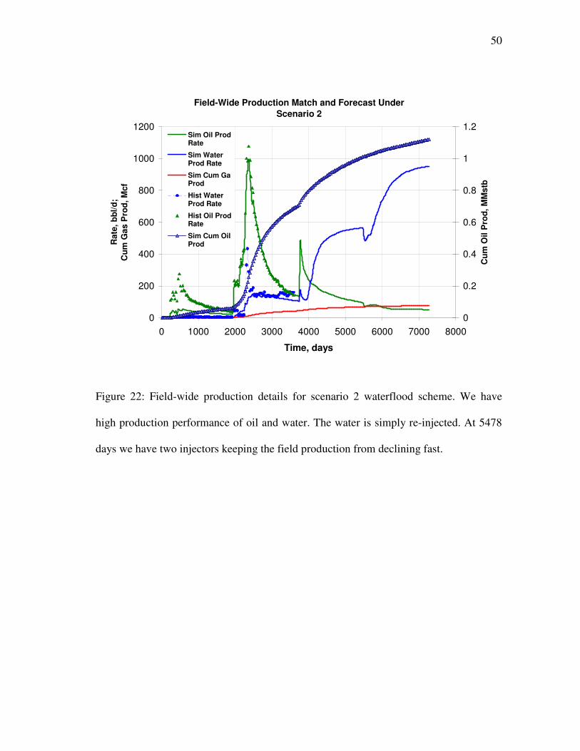
Figure 22: Field-wide production details for scenario 2 waterflood scheme. We have
high production performance of oil and water. The water is simply re-injected. At 5478
days we have two injectors keeping the field production from declining fast.
51
Field-Wide Production Match and Forecast Under
Scenario 3
0
200
400
600
800
1000
1200
0 1000 2000 3000 4000 5000 6000 7000 8000
Time, days
Ra
te,
bb
l/d
;
Cu
m G
as
Pro
d,
Mcf
0
0.2
0.4
0.6
0.8
1
1.2
Cu
m O
il P
rod
, M
Ms
tb
Sim Oil ProdRate
Sim WaterProd Rate
Sim Cum GaProd
Hist WaterProd Rate
Hist Oil ProdRate
Sim Cum OilProd
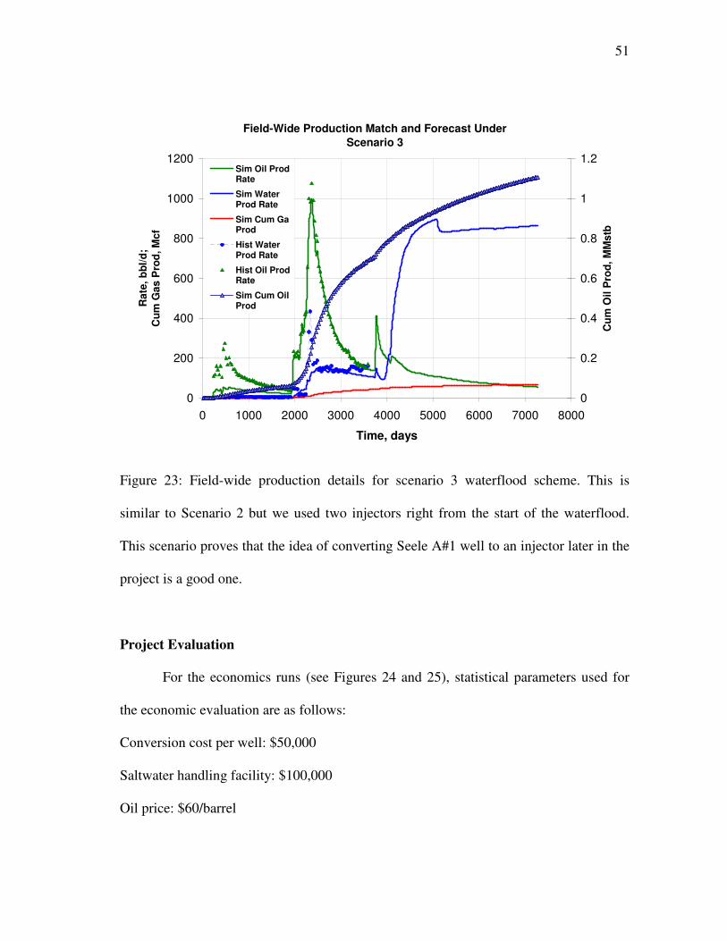
Figure 23: Field-wide production details for scenario 3 waterflood scheme. This is
similar to Scenario 2 but we used two injectors right from the start of the waterflood.
This scenario proves that the idea of converting Seele A#1 well to an injector later in the
project is a good one.
Project Evaluation
For the economics runs (see Figures 24 and 25), statistical parameters used for
the economic evaluation are as follows:
Conversion cost per well: $50,000
Saltwater handling facility: $100,000
Oil price: $60/barrel
52
Gas price: $7/Mcf
Operating costs: $2,500/well/month
Royalties: 18%, 8% overriding royalty
Discount rate: 10% per annum
Cumulative NPV of Different Scenarios Using
Field-Wide Production
-$50,000.0
$1,950,000.0
$3,950,000.0
$5,950,000.0
$7,950,000.0
$9,950,000.0
$11,950,000.0
3700 4200 4700 5200 5700 6200 6700 7200 7700
Time, days
Valu
e,
$
Scenario 2
Scenario 1
Scenario 4
Scenario 3
Scenario 5
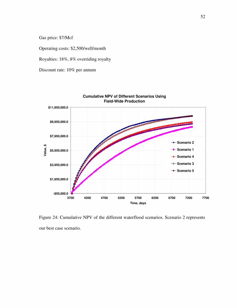
Figure 24: Cumulative NPV of the different waterflood scenarios. Scenario 2 represents
our best case scenario.
53
Scenario 1 and Scenario 2 Comparison
0
2
4
6
8
10
12
14
16
18
3700 4200 4700 5200 5700 6200 6700 7200 7700
Time, days
Oil
Pro
du
cti
on
, M
stb
0
0.2
0.4
0.6
0.8
1
1.2
1.4
1.6
Gas P
rod
uc
tio
n M
Mcf
Scenario 1Oil Production
Scenario 2 Oil Production
Scenario 1 Gas Production
Scenario 2 Gas Production
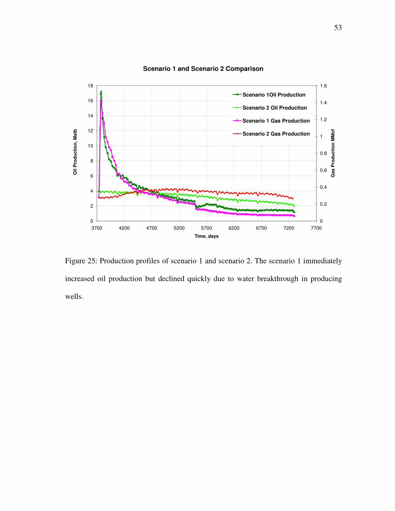
Figure 25: Production profiles of scenario 1 and scenario 2. The scenario 1 immediately
increased oil production but declined quickly due to water breakthrough in producing
wells.

54
Monte Carlo Analysis
Deterministic methods of evaluation were used during the course of this project.
However, it must be emphasize that model results are probable since there are a possible
different models that can match our historical data which everything seems to be based
off from6. A stochastic approach is used in the economics to associate probabilities with
values so the operator or investor can have certain expectations and risk evaluations.
Monte Carlo algorithm is an evaluation technique where a group of parameters
are being used in an analysis in a stochastic manner. Pseudo-random numbers are
generated for certain parameters whose values fall in within a range given by a certain
distribution. Figure 26 shows the triangular distribution which was used. This analysis
was applied on Scenario 1 by varying the oil price, the gas price, and the discount rate
using a triangular distribution.
The triangular distribution is mostly used in business decision-making when the
distribution has no certain pattern but one can confidently guess the mode, c, an upper
limit, a, and a lower limit, b. This is given by
=≤≤
−−
−
≤≤−−
−
cxaacab
ax
bxcacab
xbcbaxf
))((
)(2
))((
)(2),,|( (36)

55
Figure 26: A typical triangular distribution curve
Table 7 below shows the values used as the limits and modes for the triangular
distribution of the parameters varied in the Monte Carlo analysis.
Table 7: Economic parameters varied in the Monte Carlo analysis
parameters
limits
Oil price, $
Gas price, $
Discount rate
a 45 4 0.06
b 65 7 0.10
c 90 10 0.125
Probability Density function for a triangular distribution

56
Cumulative Distribution Plot of Scenario 2 Incremental Production
(10yr Profile)
0.00
0.10
0.20
0.30
0.40
0.50
0.60
0.70
0.80
0.90
1.00
-1000000 -500000 0 500000 1000000 1500000 2000000
NPV, $
Ex
pecta
tio
n
Figure 27: NPV plot incremental production using a 10-year production profile. This
shows an expectation of $200,000 profit as compared to doing nothing. This is because
the advantage of the waterflooding is experienced in the first 3 yrs after which the
production is less than the “do nothing” scenario.

57
Cumulative Distribution Plot of Scenario 2 Incremental Production
(5yr Profile)
0.00
0.10
0.20
0.30
0.40
0.50
0.60
0.70
0.80
0.90
1.00
0 500000 1000000 1500000 2000000 2500000 3000000 3500000
NPV, $
Ex
pecta
tio
n
Figure 28: NPV plot of incremental production using a 5-year production profile. This
time we expect a value of $1.9 million from the project. This looks more profitable
because more of the time analyzed had the waterflood case doing much better than the
“do nothing” case. This also says that the minimum profit in the short run from the
project is $1.1 million.
Conclusions and Recommendations
Understanding the geology of the Monument Field NW area is a key in the
evaluation and development of a deterministic model. Consistency and intersection of
information from different segments was achieved with good confidence. Manual
methods of history matching help build the confidence as constraints not usual for the

58
simulator under automatic methods are being used to further define the well and
reservoir properties for a better match or in some special cases a diagnosis of the well
could be obtained.
Waterflooding the Monument Northwest field is a viable option to improve the
economics of the field. The waterflood increases the field recovery by about 6% but the
improved economics is more a function of accelerated returns than of increased
recovery. The water injection increases the reservoir pressure and the performance is
improved momentarily until water breaks through in adjacent wells. Once water has
broken through, not much unswept oil can be recovered. This poses a problem for
enhancing ultimate recovery.
A Monte-Carlo analysis was used to evaluate results from different scenarios so
the time-worth and the risk of the project could be analysed. This can be seen in Figures
27 and 28. The analysis produces different results depending on the span of the project
analyzed. Results have shown that analyzing a short span of the waterflood project
presents attractive economics due to the fact that initial periods after the start of injection
has higher production performances hence better cash flow than the case of no water
injection. However, the results of a much longer time frame of the project diminishes the
attractiveness of the economics because during the later part of the time frame analyzed,
the case of no injection still has oil through-put at low cost while the initial aggressive
performance of the waterflood project has been damped due to water breakthrough.
Overall, it is still on the positive side of the economics and this makes the waterflood
project viable on different fronts.

59
NOMENCLATURE
Aq aquifer
c compressibility
C wellbore storage coefficient
Cov covariance matrix
GR gamma ray
H thickness
k permeability
p pressure
PHIA absolute porosity
PHID density porosity
PHIE effective porosity
PHIN neutron porosity
q rate
r radius
R resistivity
Rs solution gas-oil ratio
s skin
S saturation
t time

60
Symbols
t∆ time step size
x∆ gridblock size
φ porosity
µ viscosity
Subscripts
cln clean formation
D dimensionless
f flowing
i initial, counter
o oil
w water, well
s static
shl shaly formation
t true
61
REFERENCES
1. North, F.K.1985. Petroleum Geology, Boston: Allen Unwin.
2. Dunham, R. J. and Folk, R. L.1962. Classification of Carbonate Rocks
According to Depositional Texture. In Classification of Carbonate Rocks, ed.
W.E. Ham, Chap. 2, 6-9. AAPG Memoir 1. Tulsa: American Association of
Petroleum Geologists.
3. Foster, N. and Beaumont, E.1990. Formation Evaluation II: Log
Interpretation, AAPG Reprint Series, AAPG, Tulsa 17: 69-71.
4. Ahr, W.M. 2007. Carbonate Reservoir Geology Class notes, Texas A&M
University, College Station.
5. Byrnes, A.P. and Bhattacharya, S. 2006. Influence of Initial and Residual Oil
Saturation and Relative Permeability on Recovery from Transition Zone
Reservoirs in Shallow Shelf Carbonates. Paper SPE 99736 presented at the
2006 SPE/DOE Symposium on Improved Oil Recovery, Tulsa, Oklahoma,
22-26 April.
6. Rietz, D. and Usmani, A. 2005. Reservoir Simulation and Reserves
Classifications -Guidelines for Reviewing Model History Matches to Help
Bridge the Gap Between Evaluators and Simulation Specialists. Paper SPE
96410 presented at the 2005 SPE Annual Technical Conference and
Exhibition, Dallas, 9-12 October.
62
7. Tucker, M.E. and Bathurst, R.G.1990. Carbonate Diagenesis, Oxford:
BlackWell Scientific Publication.
8. Wilson, J.L. 1975. Carbonate Facies in Geologic History. Berlin: Springer-
Verlag.
9. Ahr, W.M. 1973. The Carbonate Ramp - An Alternative to the Shelf Model.
Trans., Gulf Coast Association of Geological Societies Vol. 23: 221-225.
10. Lee, W.J., Rollins, B. J. and Spivey, J.P. 1997. Well Testing, Textbook
Series, SPE, Richardson, Texas: 151-154.
11. Correa, F. A. and Ramey, H.J. 1987. A Method for Pressure Buildup
Analysis of Drillstem Tests. Paper SPE 16802 presented at the SPE Annual
Technical Conference and Exhibition, Dallas, 27-30 September.
12. Warren, J.E and Root, P.J. The Behavior of Naturally Fractured Reservoirs.
SPE Journal (Sept. 1963) 52-53.
13. Bahar, A. and Kelkar, M. 1998. Journey From Well Logs/Cores to Integrated
Geological and Petrophysical Simulation: A Methodology and Application.
Paper SPE 39565 presented at the 1998 SPE India Oil and Gas Conference
and Exhibition, New Delhi, 17-19 February.
14. Aufricht, W.R. and Koepf E.H. 1957. The Interpretation of Capillary
Pressure Data from Carbonate Reservoirs. Revised Manuscript SPE 826-G
available from SPE, Richardson, Texas.
15. Carter, R.D. and Tracy, G.W. 1960. An Improved Method for Calculating
Water Influx, Trans., AIME 219, 156.

63
16. Wattenbarger, R.A. 2006. Advanced Reservoir Engineering class notes,
Texas A&M University, College Station.
17. Peaceman, D.W. 1977. Interpretation of Well-Block Pressures in Numerical
Reservoir Simulation. Paper SPE 6893 presented at the SPE-AIME 52nd
Annual Technical Conference and Exhibition, Denver, 9-12 October.
18. Gang, T. and Kelkar, M. 2006. Efficient History Matching in Naturally
Fractured Reservoirs. Paper SPE 99578 presented at the 2006 SPE/DOE
Symposium on Improved Oil Recovery, Tulsa, 22-26 April.
19. Willhite, G. P. 1986. Waterflooding, Textbook Series, SPE, Richardson,
Texas, 36-39.
20. Economides, M. J., Oligney, R. E. and Valko, P. 2002. Unified Fracture
Design: Bridging the Gap Between Theory and Practice, 21. Alvin, Texas:
Orsa Press.
21. Valko, P. and Economides, M. 1995. Hydraulic Fracture Mechanics, New
York: Wiley Chichester.

64
APPENDIX A
DIAGRAMMATIC REPRESENTATION OF THE MONUMENT NORTHWEST
FIELD
Figure A1: 3D reservoir model of the Monument NW field showing wells. The blue
areas show acreage extension to account for two Anderson Wells perforated into those
zones.
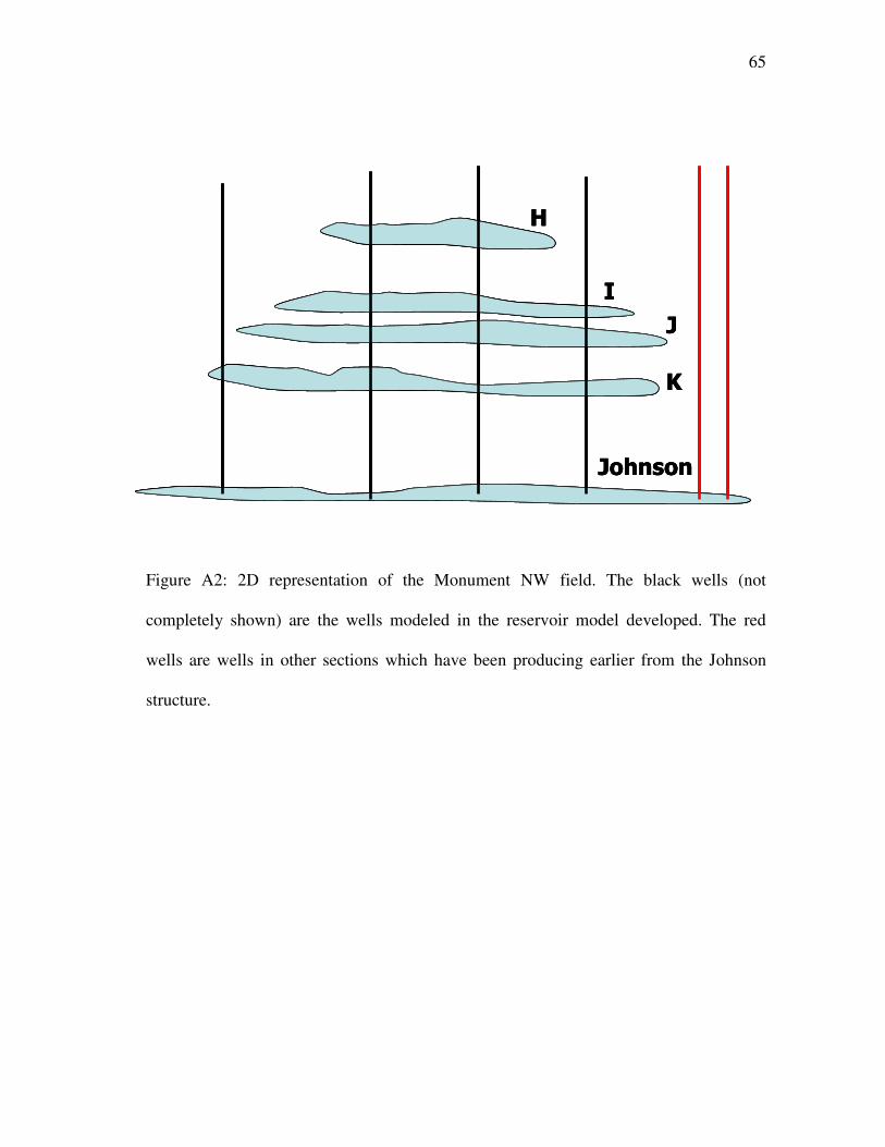
65
Figure A2: 2D representation of the Monument NW field. The black wells (not
completely shown) are the wells modeled in the reservoir model developed. The red
wells are wells in other sections which have been producing earlier from the Johnson
structure.
H
I
J
K
Johnson
H
I
J
K
Johnson
H
I
J
K
Johnson
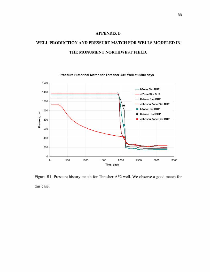
66
APPENDIX B
WELL PRODUCTION AND PRESSURE MATCH FOR WELLS MODELED IN
THE MONUMENT NORTHWEST FIELD.
Pressure Historical Match for Thrasher A#2 Well at 3300 days
0
200
400
600
800
1000
1200
1400
1600
0 500 1000 1500 2000 2500 3000 3500
Time, days
Pre
ssu
re,
psi
I-Zone Sim BHP
J-Zone Sim BHP
K-Zone Sim BHP
Johnson Zone Sim BHP
I-Zone Hist BHP
K-Zone Hist BHP
Johnson Zone Hist BHP
Figure B1: Pressure history match for Thrasher A#2 well. We observe a good match for
this case.

67
Well Production History for Thrasher A#2 Well at 3300 days
0
200
400
600
800
1000
1200
1400
0 500 1000 1500 2000 2500 3000 3500
Time, days
Pre
ss
ure
, p
si
0
5
10
15
20
25
30
35
40
45
50
Ra
te,
bb
l/d
Sim Flowing BHP
Sim Reservoir BHP
Sim Oil Production Rate
Hist Oil Production Rate
Figure B2: Well production history for Thrasher A#2 well. The flowing BHP is quite
high for this case and a further skin allocation or permeability reduction would make the
oil rate match trail off.
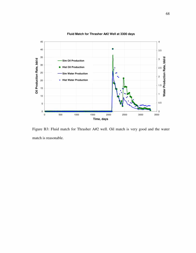
68
Fluid Match for Thrasher A#2 Well at 3300 days
0
5
10
15
20
25
30
35
40
45
0 500 1000 1500 2000 2500 3000 3500
Time, days
Oil
Pro
du
cti
on
Rate
, b
bl/
d
0
0.5
1
1.5
2
2.5
3
3.5
4
Wate
r P
rod
ucti
on
Rate
, b
bl/
d
Sim Oil Production
Hist Oil Production
Sim Water Production
Hist Water Production
Figure B3: Fluid match for Thrasher A#2 well. Oil match is very good and the water
match is reasonable.
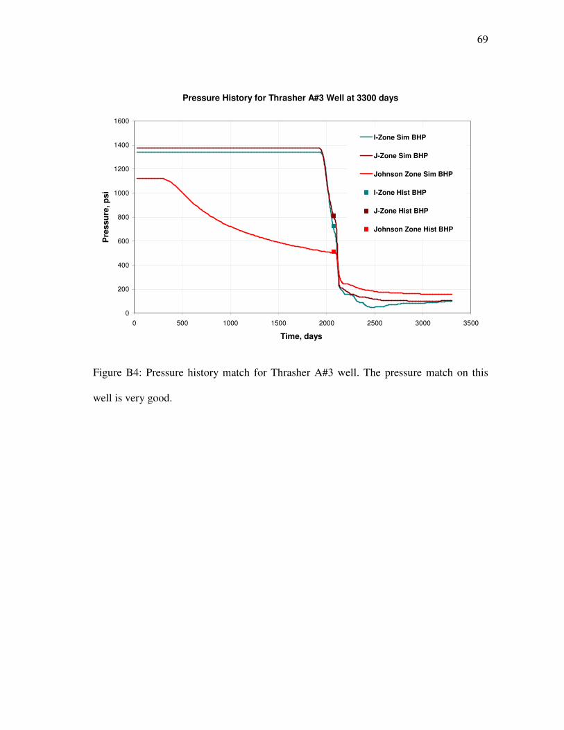
69
Pressure History for Thrasher A#3 Well at 3300 days
0
200
400
600
800
1000
1200
1400
1600
0 500 1000 1500 2000 2500 3000 3500
Time, days
Pre
ss
ure
, p
si
I-Zone Sim BHP
J-Zone Sim BHP
Johnson Zone Sim BHP
I-Zone Hist BHP
J-Zone Hist BHP
Johnson Zone Hist BHP
Figure B4: Pressure history match for Thrasher A#3 well. The pressure match on this
well is very good.

70
Well Production History for Thrasher A#3 Well at 3300 days
0
200
400
600
800
1000
1200
1400
0 500 1000 1500 2000 2500 3000 3500
Time, days
Pre
ssu
re, p
si
0
20
40
60
80
100
120
140
Ra
te, b
bl/
dSim Flowing BHP
Sim Reservoir BHP
Sim Oil Production Rate
Hist Oil Production Rate
Figure B5: Well production history for Thrasher A#3 well. We observed the well being
pumped off and this is closely simulated by the reservoir model which trails off a bit on
the oil production match.

71
Fluid History for Thrasher A#3 Well at 3300 days
0
20
40
60
80
100
120
140
0 500 1000 1500 2000 2500 3000 3500
Time, days
Oil
Pro
du
cti
on
Rate
, b
bl/
d
0
0.5
1
1.5
2
2.5
3
3.5
Wate
r P
rod
ucti
on
Ra
te,
bb
l/d
Sim Oil Production Rate
Hist Oil Production Rate
Sim Water Production Rate
Hist Water Production
Figure B6: Fluid history match for Thrasher A#3 well.
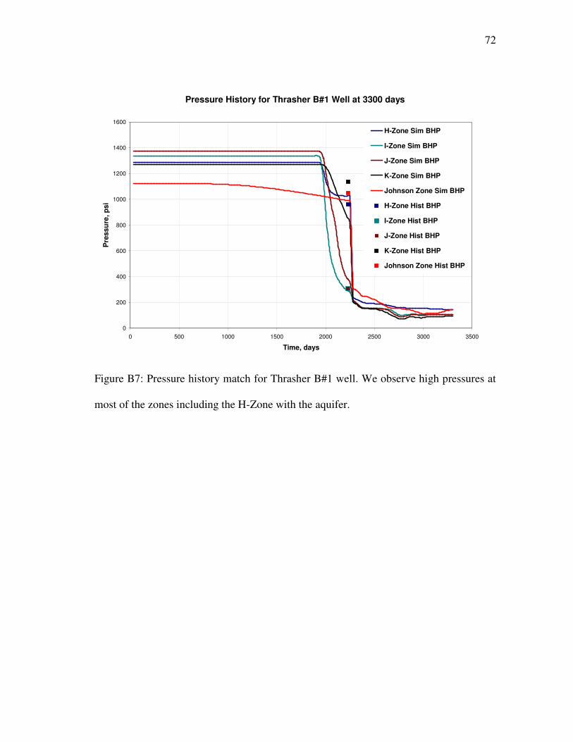
72
Pressure History for Thrasher B#1 Well at 3300 days
0
200
400
600
800
1000
1200
1400
1600
0 500 1000 1500 2000 2500 3000 3500
Time, days
Pre
ssu
re,
psi
H-Zone Sim BHP
I-Zone Sim BHP
J-Zone Sim BHP
K-Zone Sim BHP
Johnson Zone Sim BHP
H-Zone Hist BHP
I-Zone Hist BHP
J-Zone Hist BHP
K-Zone Hist BHP
Johnson Zone Hist BHP
Figure B7: Pressure history match for Thrasher B#1 well. We observe high pressures at
most of the zones including the H-Zone with the aquifer.
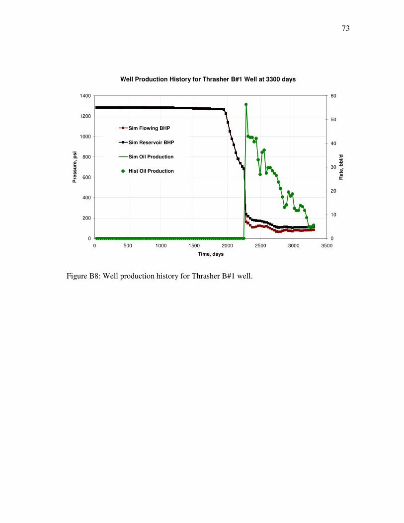
73
Well Production History for Thrasher B#1 Well at 3300 days
0
200
400
600
800
1000
1200
1400
0 500 1000 1500 2000 2500 3000 3500
Time, days
Pre
ss
ure
, p
si
0
10
20
30
40
50
60
Rate
, b
bl/
d
Sim Flowing BHP
Sim Reservoir BHP
Sim Oil Production
Hist Oil Production
Figure B8: Well production history for Thrasher B#1 well.
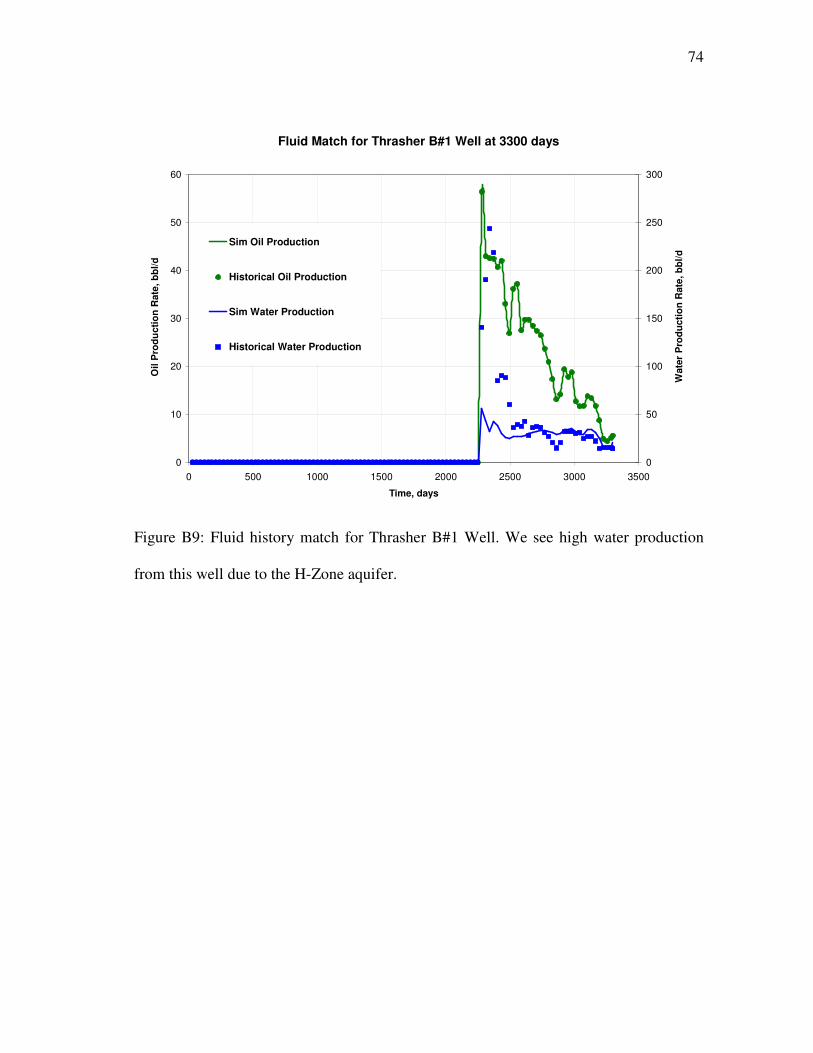
74
Fluid Match for Thrasher B#1 Well at 3300 days
0
10
20
30
40
50
60
0 500 1000 1500 2000 2500 3000 3500
Time, days
Oil
Pro
du
cti
on
Rate
, b
bl/
d
0
50
100
150
200
250
300
Wate
r P
rod
ucti
on
Rate
, b
bl/
d
Sim Oil Production
Historical Oil Production
Sim Water Production
Historical Water Production
Figure B9: Fluid history match for Thrasher B#1 Well. We see high water production
from this well due to the H-Zone aquifer.
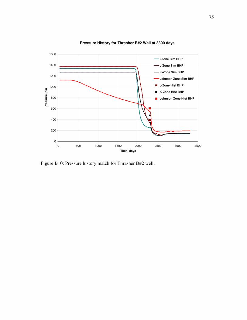
75
Pressure History for Thrasher B#2 Well at 3300 days
0
200
400
600
800
1000
1200
1400
1600
0 500 1000 1500 2000 2500 3000 3500
Time, days
Pre
ss
ure
, p
si
I-Zone Sim BHP
J-Zone Sim BHP
K-Zone Sim BHP
Johnson Zone Sim BHP
J-Zone Hist BHP
K-Zone Hist BHP
Johnson Zone Hist BHP
Figure B10: Pressure history match for Thrasher B#2 well.
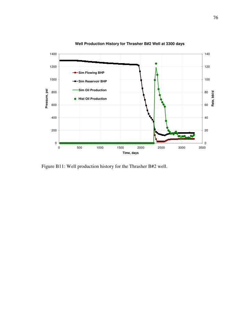
76
Well Production History for Thrasher B#2 Well at 3300 days
0
200
400
600
800
1000
1200
1400
0 500 1000 1500 2000 2500 3000 3500
Time, days
Pre
ssu
re,
psi
0
20
40
60
80
100
120
140
Ra
te,
bb
l/d
Sim Flowing BHP
Sim Reservoir BHP
Sim Oil Production
Hist Oil Production
Figure B11: Well production history for the Thrasher B#2 well.
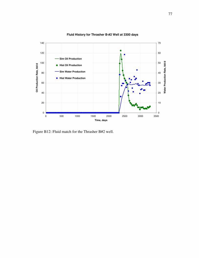
77
Fluid History for Thrasher B-#2 Well at 3300 days
0
20
40
60
80
100
120
140
0 500 1000 1500 2000 2500 3000 3500
Time, days
Oil
Pro
du
cti
on
Rate
, b
bl/
d
0
10
20
30
40
50
60
70
Wate
r P
rod
ucti
on
Rate
, b
bl/
d
Sim Oil Production
Hist Oil Production
Sim Water Production
Hist Water Production
Figure B12: Fluid match for the Thrasher B#2 well.
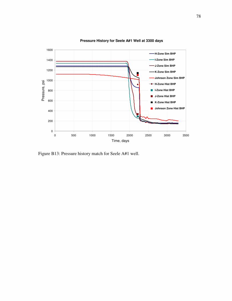
78
Pressure History for Seele A#1 Well at 3300 days
0
200
400
600
800
1000
1200
1400
1600
0 500 1000 1500 2000 2500 3000 3500
Time, days
Pre
ssu
re,
psi
H-Zone Sim BHP
I-Zone Sim BHP
J-Zone Sim BHP
K-Zone Sim BHP
Johnson Zone Sim BHP
H-Zone Hist BHP
I-Zone Hist BHP
J-Zone Hist BHP
K-Zone Hist BHP
Johnson Zone Hist BHP
Figure B13: Pressure history match for Seele A#1 well.

79
Well Production History for Seele A#1 Well at 3300 days
0
200
400
600
800
1000
1200
1400
0 500 1000 1500 2000 2500 3000 3500
Time, days
Pre
ss
ure
, p
si
0
20
40
60
80
100
120
140
160
180
Ra
te,
bb
l/d
Flowing BHP
Sim Reservoir BHP
Sim Oil Production
Hist Oil Production Rate
Figure B14: Well production history for Seele A#1 well.
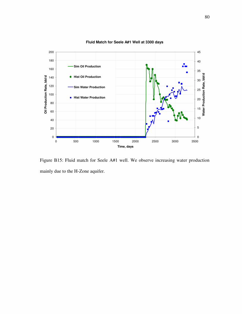
80
Fluid Match for Seele A#1 Well at 3300 days
0
20
40
60
80
100
120
140
160
180
200
0 500 1000 1500 2000 2500 3000 3500
Time, days
Oil
Pro
du
cti
on
Ra
te,
bb
l/d
0
5
10
15
20
25
30
35
40
45
Wate
r P
rod
uc
tio
n R
ate
, b
bl/
d
Sim Oil Production
Hist Oil Production
Sim Water Production
Hist Water Production
Figure B15: Fluid match for Seele A#1 well. We observe increasing water production
mainly due to the H-Zone aquifer.

81
Pressure History for Seele A#2 Well at 3300 days
0
200
400
600
800
1000
1200
1400
1600
0 500 1000 1500 2000 2500 3000 3500
Time, days
Pre
ssu
re,
psi
I-Zone Sim BHP
J-Zone Sim BHP
K-Zone Sim BHP
Johnson Zone Sim BHP
K-Zone Hist BHP
Johnson Zone Hist BHP
Figure B16: Pressure history match for Seele A#2 well.
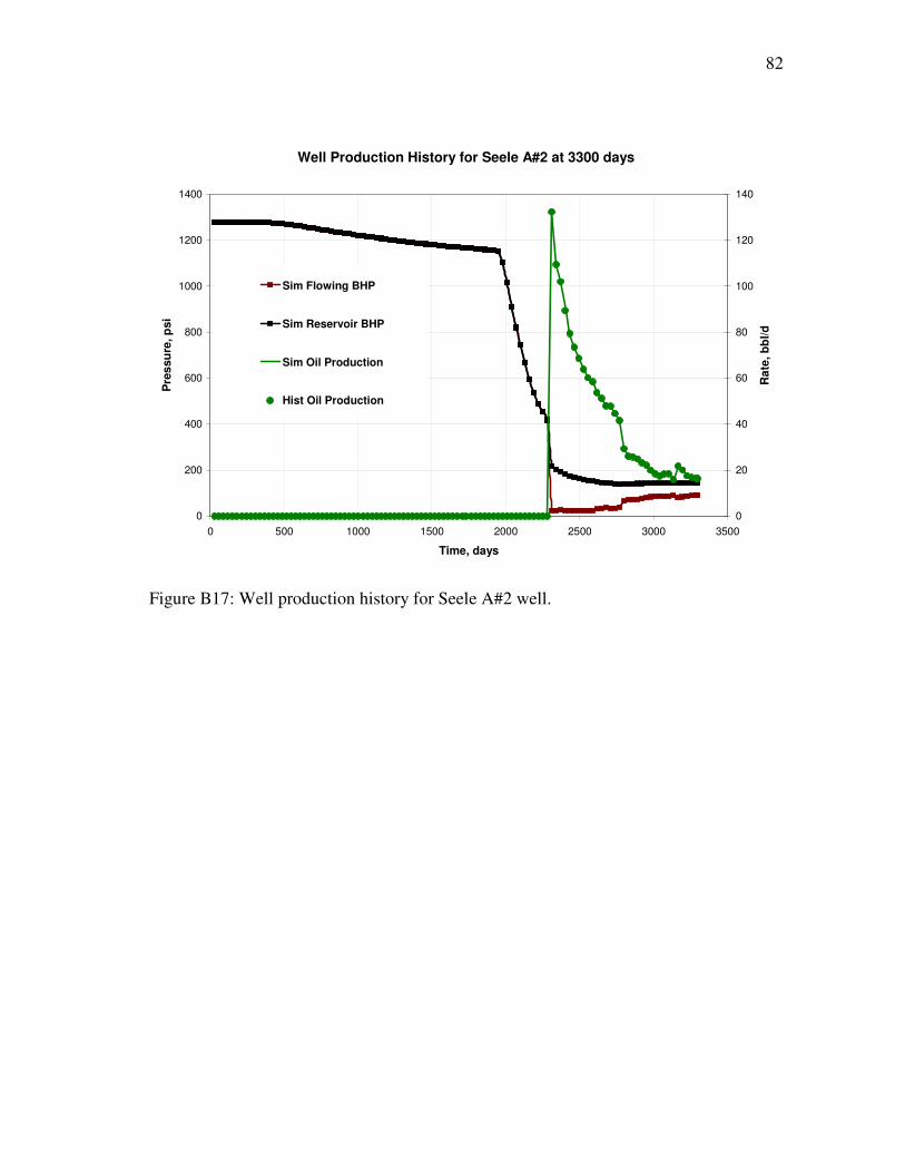
82
Well Production History for Seele A#2 at 3300 days
0
200
400
600
800
1000
1200
1400
0 500 1000 1500 2000 2500 3000 3500
Time, days
Pre
ssu
re, p
si
0
20
40
60
80
100
120
140
Ra
te, b
bl/d
Sim Flowing BHP
Sim Reservoir BHP
Sim Oil Production
Hist Oil Production
Figure B17: Well production history for Seele A#2 well.
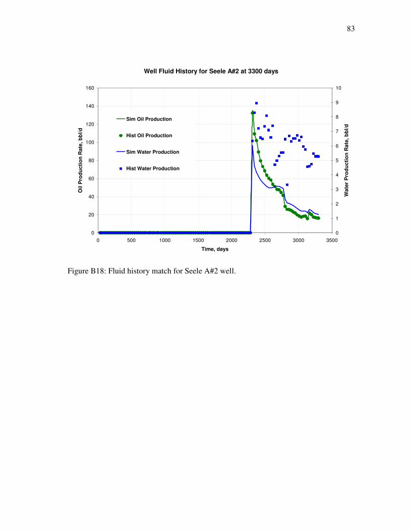
83
Well Fluid History for Seele A#2 at 3300 days
0
20
40
60
80
100
120
140
160
0 500 1000 1500 2000 2500 3000 3500
Time, days
Oil P
rod
ucti
on
Rate
, b
bl/d
0
1
2
3
4
5
6
7
8
9
10
Wa
ter
Pro
du
cti
on
Ra
te,
bb
l/d
Sim Oil Production
Hist Oil Production
Sim Water Production
Hist Water Production
Figure B18: Fluid history match for Seele A#2 well.
84
VITA
Moses Asuquo Nduonyi received his Bachelor of Engineering degree in
petroleum engineering from the University of Port Harcourt in Nigeria. He entered into
the petroleum engineering program at Texas A&M University in September 2005 and
received his Master of Science degree in December 2007. His research and work
interests include reservoir modeling and pressure transient analysis with a view to
enhanced oil recovery.
Mr. Nduonyi may be reached at iValue Consulting, 1501 Holleman Drive
College Station, TX 77840. His email is [email protected].