Integrated Genome Browser User’s Guide - SourceForgegenoviz.sourceforge.net/IGB_User_Guide.pdf ·...
108
1 Integrated Genome Browser User’s Guide October 2009 IGB User’s Guide 1
Transcript of Integrated Genome Browser User’s Guide - SourceForgegenoviz.sourceforge.net/IGB_User_Guide.pdf ·...
1
Integrated Genome Browser User’s Guide
October 2009
IGB User’s Guide 1
2
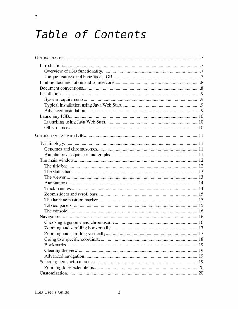
Table of Contents
GETTING STARTED....................................................................................................................7
Introduction......................................................................................................................7Overview of IGB functionality....................................................................................7Unique features and benefits of IGB...........................................................................7
Finding documentation and source code..........................................................................8Document conventions.....................................................................................................8Installation........................................................................................................................9
System requirements....................................................................................................9Typical installation using Java Web Start....................................................................9Advanced installation...................................................................................................9
Launching IGB...............................................................................................................10Launching using Java Web Start................................................................................10Other choices.............................................................................................................10
GETTING FAMILIAR WITH IGB..................................................................................................11
Terminology...................................................................................................................11Genomes and chromosomes......................................................................................11Annotations, sequences and graphs...........................................................................11
The main window..........................................................................................................12The title bar................................................................................................................12The status bar.............................................................................................................13The viewer.................................................................................................................13Annotations................................................................................................................14Track handles.............................................................................................................14Zoom sliders and scroll bars......................................................................................15The hairline position marker......................................................................................15Tabbed panels............................................................................................................15The console................................................................................................................16
Navigation......................................................................................................................16Choosing a genome and chromosome.......................................................................16Zooming and scrolling horizontally...........................................................................17Zooming and scrolling vertically...............................................................................17Going to a specific coordinate...................................................................................18Bookmarks.................................................................................................................19Clearing the view.......................................................................................................19Advanced navigation.................................................................................................19
Selecting items with a mouse.........................................................................................19Zooming to selected items.........................................................................................20
Customization................................................................................................................20
IGB User’s Guide 2

3
Opening tab panels in new windows.........................................................................20Keyboard shortcuts....................................................................................................21Customizing display properties..................................................................................21Setting preferences.....................................................................................................21
LOADING ANNOTATIONS...........................................................................................................22
Data sources...................................................................................................................22Loading annotations from Servers.................................................................................22QuickLoad......................................................................................................................23DAS servers...................................................................................................................24
Loading from DAS/1.................................................................................................24Loading from DAS/2.................................................................................................24
Loading annotations from files......................................................................................25Merging with current genome....................................................................................26Viewing in a new genome..........................................................................................26Annotation file formats..............................................................................................26
Details for selected features...........................................................................................27Links to public web sites................................................................................................28
WORKING WITH SEQUENCE RESIDUES.........................................................................................29
Loading sequences.........................................................................................................29Loading from a file....................................................................................................29
Viewing sequence residues............................................................................................30Copying sequence bases................................................................................................31
SEARCHING............................................................................................................................32
Finding an annotation by name......................................................................................32Finding sequence patterns..............................................................................................32
Finding instances of a known sequence.....................................................................33Finding instances of a sequence containing unknowns.............................................33
CUSTOMIZING ANNOTATION TRACKS...........................................................................................35
Changing the width of track handles.............................................................................35Reordering tracks toptobottom .................................................................................36Selecting tracks..............................................................................................................36Changing track properties..............................................................................................36Changing annotation colors...........................................................................................37Changing track names....................................................................................................37Hiding and showing annotation tracks...........................................................................37Hiding and showing strands...........................................................................................37Collapsing and expanding tracks...................................................................................38Setting a row limit .........................................................................................................38Removing the row limit.................................................................................................39Using annotation id labels..............................................................................................39Using color to represent scores......................................................................................40
IGB User’s Guide 3
4
TOOLS FOR COMPARING ANNOTATIONS.......................................................................................41
Highlighting matching endpoints...................................................................................41Slicing............................................................................................................................41
Viewing deletions and insertions...............................................................................42Disabling the sliced view...........................................................................................43Adjusting the sliced view...........................................................................................43
Summarizing tracks.......................................................................................................43Looking at density of annotation coverage....................................................................44Combining tracks...........................................................................................................45
WORKING WITH GRAPHS..........................................................................................................48
Introduction....................................................................................................................48Loading graph files........................................................................................................49Changing graph appearance...........................................................................................50
Change the height of a graph.....................................................................................50Change graph styles...................................................................................................51Change graph color....................................................................................................57Change scale..............................................................................................................57
Hiding and deleting graphs............................................................................................58Advanced graph manipulations......................................................................................59
Graph labeling............................................................................................................59Floating graphs...........................................................................................................59Transforming to a nonlinear scale............................................................................60Duplicating graphs.....................................................................................................60Joining and splitting graphs.......................................................................................60Graph arithmetic........................................................................................................61
Applying thresholds to graphs.......................................................................................62Using thresholding ....................................................................................................63Specify the threshold level.........................................................................................64Specify the threshold direction..................................................................................64Control gaps...............................................................................................................65Specify offsets............................................................................................................65Capture the threshold bars.........................................................................................66
Useful graph customizations..........................................................................................66Getting details about a graph.........................................................................................67Saving and bookmarking graphs....................................................................................67
Saving graph data as a file.........................................................................................67Bookmarking graph views.........................................................................................67
Printing graphs...............................................................................................................67Setting graph preferences...............................................................................................68
VISUALIZING PROBE SETS.........................................................................................................69
Introduction....................................................................................................................69Invoking IGB via links from NetAffx...........................................................................70
IGB User’s Guide 4
5
Loading probe sets from data files.................................................................................70Probes and probe sets on display...................................................................................71
Probe set design sequence..........................................................................................71Probes and probe sets.................................................................................................72Probe set labels..........................................................................................................73Polyadenylation sites ...............................................................................................73Recognizing putative probe set targets......................................................................73
Getting more information for a probe set......................................................................73About alignments...........................................................................................................73
Probe mappings..........................................................................................................73Viewing tips...................................................................................................................74
CAPTURING, SAVING, AND SHARING DATA...................................................................................75
Viewing a region in the UCSC browser .......................................................................75Saving annotation tracks................................................................................................75Copying sequence bases................................................................................................75Saving graph files..........................................................................................................76Bookmarking..................................................................................................................76
Creating bookmarks...................................................................................................76Using bookmarks.......................................................................................................76Viewing and changing bookmark details...................................................................76Exporting bookmarks.................................................................................................77Importing bookmarks.................................................................................................77
Copying data from table cells........................................................................................77Printing...........................................................................................................................77
CONFIGURING DATA SOURCES...................................................................................................79
Add Server.....................................................................................................................79Synonyms.......................................................................................................................80The file cache.................................................................................................................81
ADVANCED FEATURES.............................................................................................................82
Clamping on a view.......................................................................................................82Shrinkwrapping............................................................................................................83Showing ORFs and stop codons ...................................................................................83
Clearing ORFs from the viewer.................................................................................84Identifying a translation frame...................................................................................84
Interacting with other genome browsers........................................................................85Track lines......................................................................................................................85Controlling IGB through a browser...............................................................................86
APPENDIX 1 JAVA WEB START...............................................................................................88
Troubleshooting.............................................................................................................88Web Start Console.........................................................................................................89
APPENDIX 2 TROUBLESHOOTING..............................................................................................91
IGB User’s Guide 5
6
Troubleshooting specific areas......................................................................................91IGB seems slow or sluggish.......................................................................................91Keyboard shortcut command doesn’t work...............................................................91Out of memory errors.................................................................................................92Tab or tab window is missing....................................................................................92Tier labels don't lineup with tiers.............................................................................92You can't see all the tiers...........................................................................................92Reverse strand data appears above the axis...............................................................92
General troubleshooting.................................................................................................92
APPENDIX 3 PREFERENCES......................................................................................................94
Importing and exporting preferences.............................................................................94Exporting preference settings....................................................................................94Importing preference settings....................................................................................95
Customizing the default appearance of tracks...............................................................95Changing the name of the track.................................................................................96Changing the color of annotations.............................................................................96Changing the background color of the track..............................................................96Displaying both strands in one track or two..............................................................96Collapsing annotation rows into a single row............................................................96Setting the maximum number of annotation rows to display....................................96Grouping exons..........................................................................................................97Choosing annotation id labels....................................................................................97
Changing keyboard commands......................................................................................98Setting graph preferences...............................................................................................98Setting color and axis display preferences.....................................................................99
Setting axis display – option descriptions..................................................................99Setting ORF and stopcodon colors...........................................................................99Setting other options................................................................................................100
LICENSE..............................................................................................................................101
INDEX.................................................................................................................................105
IGB User’s Guide 6
7
Getting started
IntroductionThe Integrated Genome Browser (IGB) is a powerful tool to help genome researchers:
➢ Compare experimental results to computational results
➢ Visualize and compare multiple genomic annotation sets from a variety of public and private sources
➢ Target areas of interest to explore further via other tools and/or experimentation
➢ Provide guidance for finetuning or modification of experiments
Overview of IGB functionalityGenerally, use IGB to:
➢ Select and load genomic annotations to analyze from a variety of sources including your own experimental results
➢ Compare variations in annotations and expression activity in different data sets
➢ Search for and drill down in areas of interest
Unique features and benefits of IGBIGB combines in one viewer your own experimental or computational results, common reference information, and access to public and private data banks.
Other features unique to IGB include:
➢ A slicing tool that facilitates examination and manipulation of alternate splicings, intron and exon boundaries
➢ Ability to view graphs of scores at specified points along the genome in the same view as genomic annotations
➢ Facility in handling large amounts of genomic annotations with speed and efficiency
➢ Can be controlled from a web browser or any other program capable of sending HTTP requests
➢ Runs on multiple platforms, including Windows, Linux and Macintosh
➢ The entire program, including all thirdparty components, is opensource and written in Java
➢ The license allows all of part of the program to be incorporated into derivative applications
IGB User’s Guide 7
8
Finding documentation and source codeIGB is part of the open source GenoViz project. Links to all documentation and Java source code for IGB, including the most recent version of this document, can be found on the home page for the GenoViz project: http://genoviz.sourceforge.net/ There are also links to discussion forums and ways to provide feedback.
Guides for using data from various Affymetrix programs are available on the Affymetrix Tools web page: http://www.affymetrix.com/support/developer/tools/affytools.affx
and on the Affymetrix Developer’s Network web page: http://www.affymetrix.com/support/developer/tools/devnettools.affx.
Those pages contain information for dealing with data from these sources, among others:
➢ GCOS
➢ CNAT
➢ Expression Console
➢ Tiling Analysis Software
➢ NetAffx
Document conventionsOnscreen text (i.e., menus, button labels, folder names, field values, etc.) is indicated by Arial font.
An item followed by a “greater than” symbol followed by another item means “click the first item; the second item will become visible; then click the second item.”
Examples:
➢ File menu > Open File means “click on the File menu and choose Open File.”
➢ QuickLoad tab > Load Sequence Residues means “click the QuickLoad tab and then click the Load Sequence Residues button”
Screen shots were current at the time this document was prepared. Small changes in the locations or names of controls may occur as IGB evolves through different versions. Since IGB can be run on multiple operating systems with different lookandfeel conventions, the appearance of the screen shots may not exactly match what appears on your screen.
Unless otherwise noted, all commands are described as used on the Linux operating system. Minor differences sometimes occur on different operating systems. Operations in this document that require rightclicking can be performed on a Macintosh with a singlebutton mouse by holding down the control key while clicking the mouse.
IGB User’s Guide 8
9
Installation
System requirementsIGB can be used on any computer which has the Java Runtime Environment (JRE) version 1.5 or higher, installed. Version 1.6 or higher is recommended, but version 1.5 or higher is supported.
Java is available for many operating systems, including Windows, Linux, and Macintosh. Java software is free and can be installed by visiting http://java.com/
IGB is developed and tested mostly on Macintosh and Linux, but should work on any Java environment.
The amount of RAM memory and disk space required depends on the type of data you intend to view. Minimum recommendations are posted at: http://sourceforge.net/docman/?group_id=129420
Note for Macintosh users: Operations in this document that require rightclicking can be performed on Mac by holding down the control key while clicking the mouse.
Typical installation using Java Web StartTo install IGB using Java Web Start, visit: http://igb.bioviz.org/download.shtml .
If Java is properly installed on your computer, you should see one or more buttons labeled “Launch IGB”, or something similar. Simply press any of these buttons to download, install, and launch IGB.
If IGB has not already been installed, or if an update is available, the most current version will be installed automatically. If IGB has already been installed, pressing these buttons will simply start the program that is already installed on your machine.
If you did not see one or more buttons labeled “Launch IGB”, you need to install Java Web Start, which is included with current versions of the Java Runtime Engine. (See System requirements above.)
After Java Web Start is installed, close and restart your browser, then return to the web page mentioned above and press one of the buttons labeled “Launch IGB”.
Advanced installationAdvanced users may choose to install IGB without using Java Web Start. This is appropriate for developers who wish to view or extend the source code, and for advanced users who are willing to forgo the automatic updating
IGB User’s Guide 9
10
provided by Java Web Start. These other installation options are described at http://genoviz.sourceforge.net/.
Launching IGBThe procedure used for launching IGB will depend on whether you installed with the typical method described in Typical installation using Java WebStart on page 9 or one of the methods described in Advanced installation on page 9.
Regardless of which method you use, launching multiple instances of IGB simultaneously is not recommended. (This is because IGB saves various settings, including your bookmarks, on your disk. If two instances of IGB are reading and writing those same files, the results are unpredictable.)
Launching using Java Web StartIf you installed IGB using the method in Typical installation using Java WebStart launch IGB using one of the following methods: The effect is the same regardless of which method you choose; your local copy of IGB will be updated if updates are available and will then launch.
➢ From a web browser: Return to the web site and click on one of the “Launch IGB” buttons.
Or create a web page containing the following link and click on it: http://igb.bioviz.org/download.shtml
➢ From a shortcut: If you chose to integrate IGB with your desktop environment when you installed IGB, you can launch IGB by clicking the IGB icon on your desktop or choose it from Start menu > Programs.
➢ From the Web Start console: If you did not choose to integrate IGB with your desktop environment when you installed IGB, first open the Java Web Start console.
How you open Java Web Start console varies depending on Java version and operating system. See Web Start Console on page 89.
Choose IGB in the list of applications, then click Start.
By using Java Web Start, the most current version will be downloaded and installed automatically each time you start the program. If you do not want to install the most current version of IGB, either do not use Web Start, or make sure that you are not connected to the internet when you launch IGB with Java Web Start.
The first time you launch IGB, it may need to download some data files from a central server. If you are on a slow connection, this could take a while. IGB uses a cache system to store this data on your computer so that it will load faster the next time you start the program.
IGB User’s Guide 10

11
Other choicesIf you installed IGB using the procedures described in Advanced installation, the procedure for starting IGB should have been described in the instructions that were available where you downloaded the files. Typically, you will start the program with a script named “run_igb.bat” (on Windows) or “run_igb.sh” (on Unix). Since users' computing environments vary greatly, it may be necessary to edit those startup scripts for your particular machine. Thus the use of Java Web Start is encouraged for most users.
IGB User’s Guide 11
12
Getting familiar with IGB
Terminology
Genomes and chromosomesAll data viewed in IGB, regardless of its source, is organized into distinct genomes and chromosomes.
In IGB, a chromosome refers to any single sequence. Often this will be the sequence of an actual chromosome. At other times it may be a BAC, or EST, or any other DNA sequence. All chromosomes in IGB are assumed to be DNA, rather than RNA sequences.
A genome refers to any group of these socalled chromosomes.
For example, NCBI versions 35 and 36 of the human genome are considered to be two separate genomes. Each one contains multiple chromosome sequences, including the expected chromosomes 1 to 22, X, and Y. Other sequences, such as “chr22_random” are also considered distinct chromosomes for the purposes of display in IGB.
Each sequence in IGB is identified by its genome and chromosome names, which must therefore be distinct. There can not be two genomes with the same name nor two chromosomes in one genome with the same name. Chromosomes in different genomes often do have the same name.
Unfortunately, different groups tend to refer to the same genome or chromosome by different names. Thus NCBI human genome build 35 is also known as hg17 and ensembl1834, as well as H_sapiens_May_2004. When IGB is able to recognize that two names refer to the same genome or chromosome, it will merge the data. Otherwise it will keep the two data sets distinct. Currently, IGB uses a simple table of synonyms to store these associations. You can create your own set of synonyms that will extend this set if needed. See Synonyms on page 80.
Annotations, sequences and graphsIGB can work with three distinct types of data: annotations, graphs, and genomic sequences. Some features of the program make sense only with some of these types of data.
Annotations indicate the known or suspected locations of features, such as mRNAs, exons, promoter regions, pseudogenes, and so forth. Alignments of EST sequences, GeneChip probe sequences, and other sequences to a chromosome are also treated as annotations. Annotation data can be loaded from files, QuickLoad, and DAS servers.
IGB User’s Guide 12
13
Sequences are sets of DNA residues. Although IGB is designed as a visualization program primarily for viewing annotations and graphs, sequences can also be loaded for the purpose of simple analysis and for comparison with the other data. Complex analysis of sequence data is best done in other programs. Sequences can be loaded from files, QuickLoad, and DAS servers. It is typical to load sequence data only for small regions of the genome, since it requires a great deal of RAM memory.
Graphs indicate scores or other numeric values as a function of genomic position. Graphs are generally displayed as some form of plot (x,yplot, bar plot, etc.). The results from GeneChip tiling arrays and from chromosome copy number analysis are generally represented as graphs. Simple graphs represent values for individual genomic positions. Interval graphs represent values for ranges of genomic positions. Graph data is generally loaded from files.
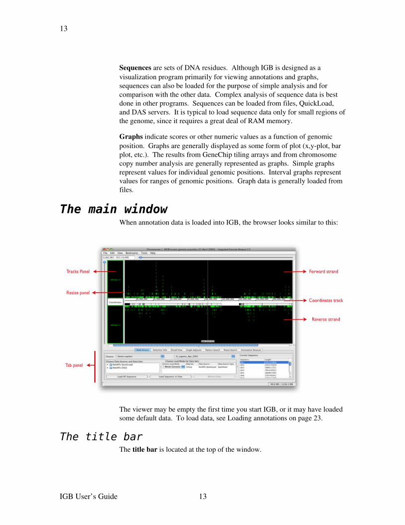
The main windowWhen annotation data is loaded into IGB, the browser looks similar to this:
The viewer may be empty the first time you start IGB, or it may have loaded some default data. To load data, see Loading annotations on page 23.
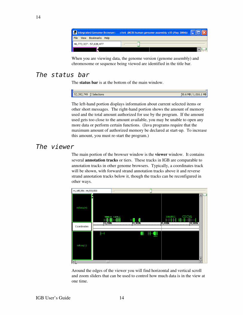
The title barThe title bar is located at the top of the window.
IGB User’s Guide 13
14
When you are viewing data, the genome version (genome assembly) and chromosome or sequence being viewed are identified in the title bar.
The status barThe status bar is at the bottom of the main window.
The lefthand portion displays information about current selected items or other short messages. The righthand portion shows the amount of memory used and the total amount authorized for use by the program. If the amount used gets too close to the amount available, you may be unable to open any more data or perform certain functions. (Java programs require that the maximum amount of authorized memory be declared at startup. To increase this amount, you must restart the program.)
The viewerThe main portion of the browser window is the viewer window. It contains several annotation tracks or tiers. These tracks in IGB are comparable to annotation tracks in other genome browsers. Typically, a coordinates track will be shown, with forward strand annotation tracks above it and reverse strand annotation tracks below it, though the tracks can be reconfigured in other ways.
Around the edges of the viewer you will find horizontal and vertical scroll and zoom sliders that can be used to control how much data is in the view at one time.
IGB User’s Guide 14
15
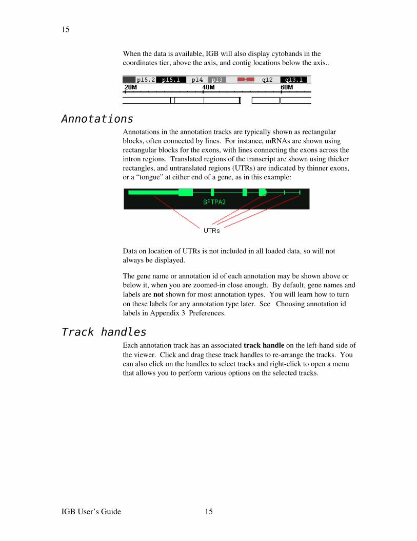
When the data is available, IGB will also display cytobands in the coordinates tier, above the axis, and contig locations below the axis..
AnnotationsAnnotations in the annotation tracks are typically shown as rectangular blocks, often connected by lines. For instance, mRNAs are shown using rectangular blocks for the exons, with lines connecting the exons across the intron regions. Translated regions of the transcript are shown using thicker rectangles, and untranslated regions (UTRs) are indicated by thinner exons, or a “tongue” at either end of a gene, as in this example:
Data on location of UTRs is not included in all loaded data, so will not always be displayed.
The gene name or annotation id of each annotation may be shown above or below it, when you are zoomedin close enough. By default, gene names and labels are not shown for most annotation types. You will learn how to turn on these labels for any annotation type later. See Choosing annotation idlabels in Appendix 3 Preferences.
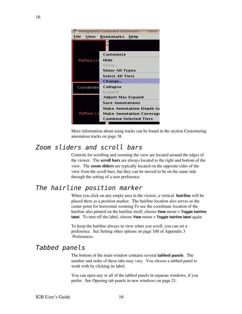
Track handlesEach annotation track has an associated track handle on the lefthand side of the viewer. Click and drag these track handles to rearrange the tracks. You can also click on the handles to select tracks and rightclick to open a menu that allows you to perform various options on the selected tracks.
IGB User’s Guide 15
16
More information about using tracks can be found in the section Customizingannotation tracks on page 38.
Zoom sliders and scroll barsControls for scrolling and zooming the view are located around the edges of the viewer. The scroll bars are always located to the right and bottom of the view. The zoom sliders are typically located on the opposite sides of the view from the scroll bars, but they can be moved to be on the same side through the setting of a user preference.
The hairline position markerWhen you click on any empty area in the viewer, a vertical hairline will be placed there as a position marker. The hairline location also serves as the center point for horizontal zooming.To see the coordinate location of the hairline also printed on the hairline itself, choose View menu > Toggle hairline label. To turn off the label, choose View menu > Toggle hairline label again.
To keep the hairline always in view when you scroll, you can set a preference. See Setting other options on page 100 of Appendix 3 Preferences.
Tabbed panelsThe bottom of the main window contains several tabbed panels. The number and order of these tabs may vary. You choose a tabbed panel to work with by clicking its label.
You can open any or all of the tabbed panels in separate windows, if you prefer. See Opening tab panels in new windows on page 21.
IGB User’s Guide 16
17
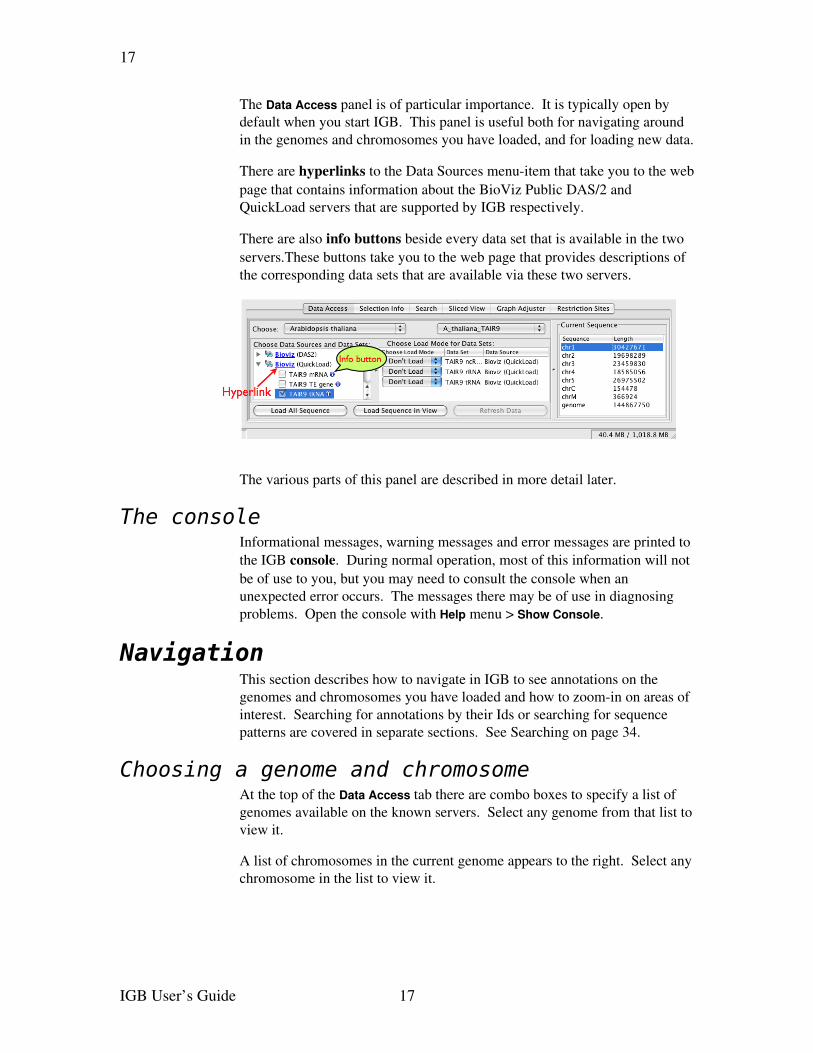
The Data Access panel is of particular importance. It is typically open by default when you start IGB. This panel is useful both for navigating around in the genomes and chromosomes you have loaded, and for loading new data.
There are hyperlinks to the Data Sources menuitem that take you to the web page that contains information about the BioViz Public DAS/2 and QuickLoad servers that are supported by IGB respectively.
There are also info buttons beside every data set that is available in the two servers.These buttons take you to the web page that provides descriptions of the corresponding data sets that are available via these two servers.
The various parts of this panel are described in more detail later.
The consoleInformational messages, warning messages and error messages are printed to the IGB console. During normal operation, most of this information will not be of use to you, but you may need to consult the console when an unexpected error occurs. The messages there may be of use in diagnosing problems. Open the console with Help menu > Show Console.
NavigationThis section describes how to navigate in IGB to see annotations on the genomes and chromosomes you have loaded and how to zoomin on areas of interest. Searching for annotations by their Ids or searching for sequence patterns are covered in separate sections. See Searching on page 34.
Choosing a genome and chromosomeAt the top of the Data Access tab there are combo boxes to specify a list of genomes available on the known servers. Select any genome from that list to view it.
A list of chromosomes in the current genome appears to the right. Select any chromosome in the list to view it.
IGB User’s Guide 17
18
To see data for a genome that is not already loaded, you will need to load the data, either from QuickLoad, from a DAS server, or from a data file. See Loading annotations on page 23. Any genomes that are loaded will then appear in the pulldown list and can be selected in future.
Zooming and scrolling horizontallyThe horizontal zoom slider is located along the top (or bottom) edge of the viewer. To zoom in, move the zoom slider to the right. To zoom out, move the zoom slider to the left.
The hairline marks the focus of horizontal zooming. Click in any empty position in the view to reset the hairline position and thus reset the center of zooming.
When you are zoomed in, you can scroll through the view in several ways:
➢ Use the horizontal scroll box slider at the bottom of the viewer panel to scroll along the sequence. Slider size and speed of movement will vary according to the current zoom level.
➢ Click in the scroll bar trough on either side of the slider to move it in the direction of your click.
➢ For finest precision when zoomed in, click the arrows at the ends of the scroll bar.
When you are zoomed all the way out (the horizontal zoom control slider is at the far left), you are already viewing the entire range of the loaded data and the scroll box slider is not available.
You can also set IGB to automatically scroll along the chromosome. This is useful occasionally for presentations. Choose View menu > AutoScroll.
Zooming and scrolling verticallyZooming and scrolling vertically are similar to zooming and scrolling horizontally. Zooming vertically is especially useful for viewing ESTs or any other annotation types with many rows of annotations. (You will later see how to collapse or even hide tracks with too many rows of annotations. See Customizing annotation tracks on page 38)
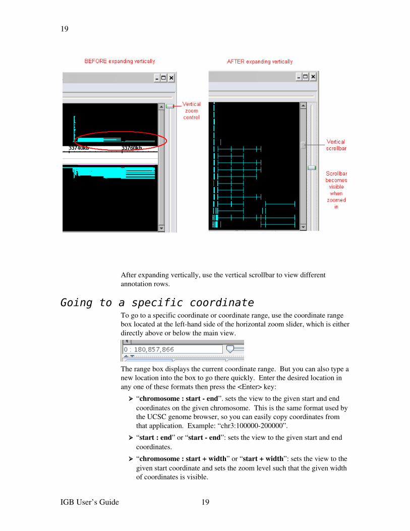
The vertical zoom slider is located immediately to the left (or right) of the main view. To zoom the view vertically, drag the vertical slider down:
IGB User’s Guide 18
19
After expanding vertically, use the vertical scrollbar to view different annotation rows.
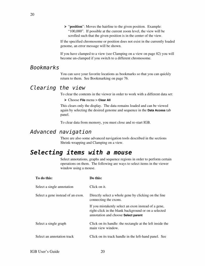
Going to a specific coordinateTo go to a specific coordinate or coordinate range, use the coordinate range box located at the lefthand side of the horizontal zoom slider, which is either directly above or below the main view.
The range box displays the current coordinate range. But you can also type a new location into the box to go there quickly. Enter the desired location in any one of these formats then press the <Enter> key:
➢ “chromosome : start end”. sets the view to the given start and end coordinates on the given chromosome. This is the same format used by the UCSC genome browser, so you can easily copy coordinates from that application. Example: “chr3:100000200000”.
➢ “start : end” or “start end”: sets the view to the given start and end coordinates.
➢ “chromosome : start + width” or “start + width”: sets the view to the given start coordinate and sets the zoom level such that the given width of coordinates is visible.
IGB User’s Guide 19
20
➢ “position”: Moves the hairline to the given position. Example: “100,000”. If possible at the current zoom level, the view will be scrolled such that the given position is in the center of the view.
If the specified chromosome or position does not exist in the currently loaded genome, an error message will be shown.
If you have clamped to a view (see Clamping on a view on page 82) you will become unclamped if you switch to a different chromosome.
BookmarksYou can save your favorite locations as bookmarks so that you can quickly return to them. See Bookmarking on page 76.
Clearing the viewTo clear the contents in the viewer in order to work with a different data set:
➢ Choose File menu > Clear All
This clears only the display. The data remains loaded and can be viewed again by selecting the desired genome and sequence in the Data Access tab panel.
To clear data from memory, you must close and restart IGB.
Advanced navigationThere are also some advanced navigation tools described in the sections Shrinkwrapping and Clamping on a view.
Selecting items with a mouseSelect annotations, graphs and sequence regions in order to perform certain operations on them. The following are ways to select items in the viewer window using a mouse.
To do this: Do this:
Select a single annotation Click on it.
Select a gene instead of an exon. Directly select a whole gene by clicking on the line connecting the exons.
If you mistakenly select an exon instead of a gene, rightclick in the blank background or on a selected annotation and choose Select parent
Select a single graph Click on its handle: the rectangle at the left inside the main view window.
Select an annotation track Click on its track handle in the lefthand panel. See
IGB User’s Guide 20
21
Track handles on page 15.
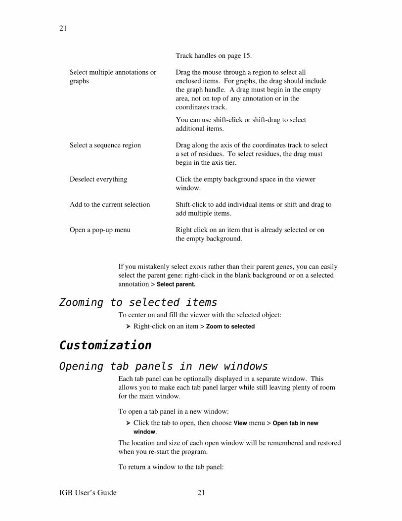
Select multiple annotations or graphs
Drag the mouse through a region to select all enclosed items. For graphs, the drag should include the graph handle. A drag must begin in the empty area, not on top of any annotation or in the coordinates track.
You can use shiftclick or shiftdrag to select additional items.
Select a sequence region Drag along the axis of the coordinates track to select a set of residues. To select residues, the drag must begin in the axis tier.
Deselect everything Click the empty background space in the viewer window.
Add to the current selection Shiftclick to add individual items or shift and drag to add multiple items.
Open a popup menu Right click on an item that is already selected or on the empty background.
If you mistakenly select exons rather than their parent genes, you can easily select the parent gene: rightclick in the blank background or on a selected annotation > Select parent.
Zooming to selected itemsTo center on and fill the viewer with the selected object:
➢ Rightclick on an item > Zoom to selected
Customization
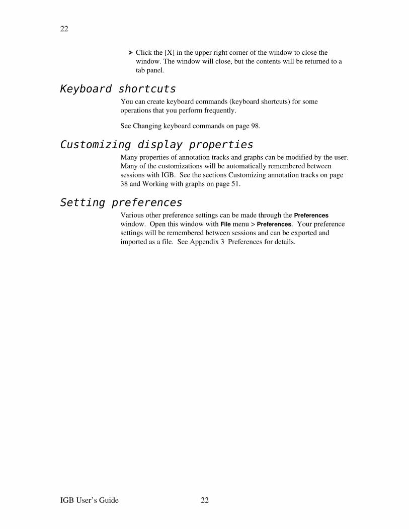
Opening tab panels in new windowsEach tab panel can be optionally displayed in a separate window. This allows you to make each tab panel larger while still leaving plenty of room for the main window.
To open a tab panel in a new window:
➢ Click the tab to open, then choose View menu > Open tab in new window.
The location and size of each open window will be remembered and restored when you restart the program.
To return a window to the tab panel:
IGB User’s Guide 21
22
➢ Click the [X] in the upper right corner of the window to close the window. The window will close, but the contents will be returned to a tab panel.
Keyboard shortcutsYou can create keyboard commands (keyboard shortcuts) for some operations that you perform frequently.
See Changing keyboard commands on page 98.
Customizing display propertiesMany properties of annotation tracks and graphs can be modified by the user. Many of the customizations will be automatically remembered between sessions with IGB. See the sections Customizing annotation tracks on page 38 and Working with graphs on page 51.
Setting preferencesVarious other preference settings can be made through the Preferences window. Open this window with File menu > Preferences. Your preference settings will be remembered between sessions and can be exported and imported as a file. See Appendix 3 Preferences for details.
IGB User’s Guide 22
23
Loading annotations
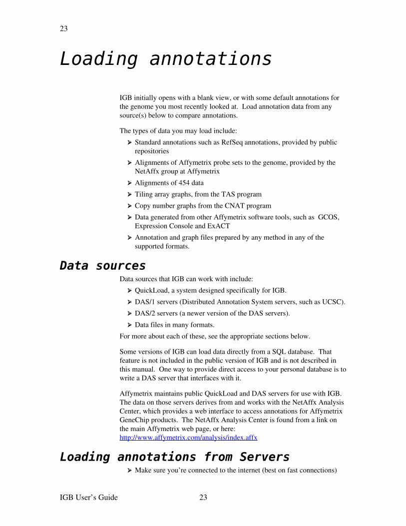
IGB initially opens with a blank view, or with some default annotations for the genome you most recently looked at. Load annotation data from any source(s) below to compare annotations.
The types of data you may load include:
➢ Standard annotations such as RefSeq annotations, provided by public repositories
➢ Alignments of Affymetrix probe sets to the genome, provided by the NetAffx group at Affymetrix
➢ Alignments of 454 data
➢ Tiling array graphs, from the TAS program
➢ Copy number graphs from the CNAT program
➢ Data generated from other Affymetrix software tools, such as GCOS, Expression Console and ExACT
➢ Annotation and graph files prepared by any method in any of the supported formats.
Data sourcesData sources that IGB can work with include:
➢ QuickLoad, a system designed specifically for IGB.
➢ DAS/1 servers (Distributed Annotation System servers, such as UCSC).
➢ DAS/2 servers (a newer version of the DAS servers).
➢ Data files in many formats.
For more about each of these, see the appropriate sections below.
Some versions of IGB can load data directly from a SQL database. That feature is not included in the public version of IGB and is not described in this manual. One way to provide direct access to your personal database is to write a DAS server that interfaces with it.
Affymetrix maintains public QuickLoad and DAS servers for use with IGB. The data on those servers derives from and works with the NetAffx Analysis Center, which provides a web interface to access annotations for Affymetrix GeneChip products. The NetAffx Analysis Center is found from a link on the main Affymetrix web page, or here: http://www.affymetrix.com/analysis/index.affx
Loading annotations from Servers➢ Make sure you’re connected to the internet (best on fast connections)
IGB User’s Guide 23

24
➢ Click the Data Access tab (already displayed by default at launch.)
See Tabbed panels on page 16.
➢ Select a species and genome version.
➢ From the tree view, select a server to use. By default, a few should be listed (including NetAffx DAS/2 and Netaffx Quickload). To add more servers, see onfiguring data sources on page 79.
➢ Available annotation types will be listed in the tree view. They will vary depending on the genome you selected. Select any of the annotation types shown in the panel by clicking the associated checkbox.
➢ The annotation type will then be displayed separately. Choose the method of loading (e.g., Region In View, Whole Genome, Full Chromosome).
➢ Choose Region In View to load annotations for the range of bases that you currently see in the viewer. Loading large ranges may take a long time if the server or your connection is slow. Loading will begin when the Refresh Data button is pressed.
➢ Whole Genome and Full Chromosome loading will begin immediately. This may take a very long time if the server or your connection is slow.
➢ RefSeq annotations and cytobands will load by default when they are available for the given genome.
➢ Wait a few moments for the annotation type to load. The data will be loaded over the internet, but a local cached copy will be made so that the data will load faster the next time.
➢ If IGB displays no annotations, choose a chromosome in the table at the right side of the Data Access tab panel. Not all annotation types will have data on all chromosomes. See Choosing a genome andchromosome on page 17.
➢ Contigs are indicated by outlined bars at the bottom of the Coordinates track. If no outlined bar is present, then there is no contig data available in the annotation type or for the region that you are viewing.
➢ (Optional) Load sequence residues for the selected chromosome. See Working with sequence residues on page 31. If the desired sequence does not appear, it may not be available for the genome you have selected.
After you have accessed a particular sequence from a particular source, IGB caches that sequence so that it loads quickly the next time you use it. To clear the cache, see The file cache on page 81.
IGB User’s Guide 24
25
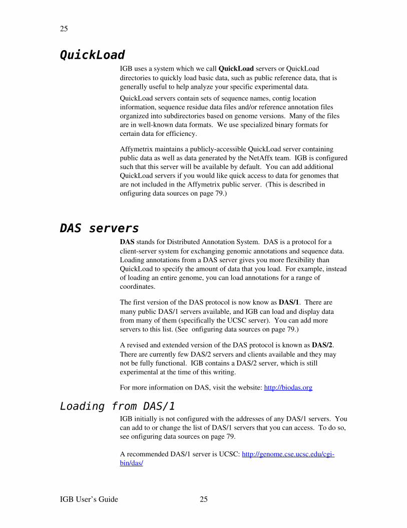
QuickLoadIGB uses a system which we call QuickLoad servers or QuickLoad directories to quickly load basic data, such as public reference data, that is generally useful to help analyze your specific experimental data.
QuickLoad servers contain sets of sequence names, contig location information, sequence residue data files and/or reference annotation files organized into subdirectories based on genome versions. Many of the files are in wellknown data formats. We use specialized binary formats for certain data for efficiency.
Affymetrix maintains a publiclyaccessible QuickLoad server containing public data as well as data generated by the NetAffx team. IGB is configured such that this server will be available by default. You can add additional QuickLoad servers if you would like quick access to data for genomes that are not included in the Affymetrix public server. (This is described in onfiguring data sources on page 79.)
DAS serversDAS stands for Distributed Annotation System. DAS is a protocol for a clientserver system for exchanging genomic annotations and sequence data. Loading annotations from a DAS server gives you more flexibility than QuickLoad to specify the amount of data that you load. For example, instead of loading an entire genome, you can load annotations for a range of coordinates.
The first version of the DAS protocol is now know as DAS/1. There are many public DAS/1 servers available, and IGB can load and display data from many of them (specifically the UCSC server). You can add more servers to this list. (See onfiguring data sources on page 79.)
A revised and extended version of the DAS protocol is known as DAS/2. There are currently few DAS/2 servers and clients available and they may not be fully functional. IGB contains a DAS/2 server, which is still experimental at the time of this writing.
For more information on DAS, visit the website: http://biodas.org
Loading from DAS/1IGB initially is not configured with the addresses of any DAS/1 servers. You can add to or change the list of DAS/1 servers that you can access. To do so, see onfiguring data sources on page 79.
A recommended DAS/1 server is UCSC: http://genome.cse.ucsc.edu/cgibin/das/
IGB User’s Guide 25
26
For information about the resources available on the UCSC server, visit http://genome.ucsc.edu/goldenPath/help/hgTracksHelp.html#IndivTracks
Loading from DAS/2IGB is initially configured with multiple DAS/2 servers. You can add to or change the list of DAS/2 servers that you can access. To do so, see onfiguring data sources on page 79.
Loading annotations from filesIGB can view data from one or more files. A variety of file formats is supported.
Data sets from different genomes are kept distinct in memory. You can switch between the data you have loaded from different genomes and chromosomes by using the pulldown genome selector and table of chromosomes in the Data Access tab panel. Refer to section Genomes andchromosomes on page 12.
Some file types already contain information specifying which genome (or occasionally genomes) they belong to. When this is the case, the file will automatically open in the specified genome and the view will be set to it. If that genome exists in your QuickLoad server, then the default RefSeq data for that genome will also be automatically opened.
Other file types do not specify which genome they belong to. In this case, you can choose to merge the file data with the current genome, or create a new genome for that data.
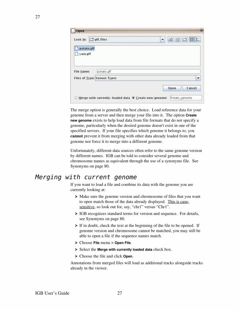
When opening a file, you must choose one of the options
➢ Merge with currentlyloaded data, or
➢ Create new genome, using a name that you provide
IGB User’s Guide 26
27
The merge option is generally the best choice. Load reference data for your genome from a server and then merge your file into it. The option Create new genome exists to help load data from file formats that do not specify a genome, particularly when the desired genome doesn't exist in one of the specified servers. If your file specifies which genome it belongs to, you cannot prevent it from merging with other data already loaded from that genome nor force it to merge into a different genome.
Unfortunately, different data sources often refer to the same genome version by different names. IGB can be told to consider several genome and chromosome names as equivalent through the use of a synonyms file. See Synonyms on page 80.
Merging with current genomeIf you want to load a file and combine its data with the genome you are currently looking at:
➢ Make sure the genome version and chromosome of files that you want to open match those of the data already displayed. This is casesensitive, so look out for, say, “chr1” versus “Chr1”.
➢ IGB recognizes standard terms for version and sequence. For details, see Synonyms on page 80.
➢ If in doubt, check the text at the beginning of the file to be opened. If genome version and chromosome cannot be matched, you may still be able to open a file if the sequence names match.
➢ Choose File menu > Open File.
➢ Select the Merge with currently loaded data check box.
➢ Choose the file and click Open.
Annotations from merged files will load as additional tracks alongside tracks already in the viewer.
IGB User’s Guide 27
28
You may need to adjust the vertical zoom level after loading new data. For instructions, see Zooming and scrolling vertically on page 18.
Viewing in a new genomeIf you want to open a single file of data and do not want to continue displaying your previously loaded data at the same time, then you can create a temporary new “genome” to hold this data.
Any genome that is already displayed in the viewer will be hidden when you use this option. But you can access that data again later by choosing that previous genome in the genome selector in the Data Access tab panel.
To open a file in a new genome:
➢ Choose File menu > Open File.
➢ Select the checkbox to Create new genome.
➢ Enter a name for this temporary genome, or accept the default name that is provided.
Annotation file formatsIGB can display several types of standard genomic file formats.
IGB can display annotations, sequences and graphs. The differences between these data types is described in Terminology on page 12. Multiple file formats exist for each of these data types. This section describes some annotation file formats. Graph file formats are discussed in the section on viewing graphs.
All filenames must include the appropriate filename extension, for example “.gff” or “.psl”.
Compressed files can only be read if a recognized filename extension is part of the filename. The filename must include both the filetype extension and the compression extension, such as “myfile.gff.zip” or “myfile.psl.gz”. Zip files must contain only a single annotation file.
➢ .zip
➢ .Z
➢ .gz
➢ .gzip
Annotation data files give sequence coordinate locations of exons, genes, transcripts, etc. on the genome. Some accepted formats are described in the table below. Others can be seen by using File menu > Open File, and seeing the list of extensions available there.
.gff There are several types of GFF files. You should identify the type of your GFF file in the header as GFF version 1, version 2, or version 3. More info is available at: http://www.sanger.ac.uk/Software/formats/GFF/index.shtml or
IGB User’s Guide 28
29
http://genome.ucsc.edu/goldenPath/help/customTrack.html#GFF
GFF version 3 is described at http://www.sequenceontology.org/gff3.shtml
.gtf For information, visit http://genome.ucsc.edu/goldenPath/help/customTrack.html#GTF
For IGB use, the track name(s) come from the source column, unless a different track name or names are specified with a track line. Coordinates will be transformed from Base 1 to Interbase 0.
.psl Displays annotations with target name matching the loaded sequence. For additional information about .psl files and how to use them, see http://hgwdev.cse.ucsc.edu/~kent/exe/doc/psLayout.doc or http://genome.ucsc.edu/goldenPath/help/customTrack.html#PSL. Files of interest are available via the DAS server.
When you load them, you will be prompted to specify whether to use the Query or Target sequence. If in doubt, use the default.
.bed Standard genomic file format. For information, visit http://genome.ucsc.edu/goldenPath/help/customTrack.html#BED
Some of those formats allow the use of track lines to control certain display properties. See Track lines on page 85.
Details for selected featuresTo get details about selected annotations or graphs:
➢ Select the item(s) of interest in the viewer.
➢ Shiftclick to select more than one item.
➢ Open the Selection Info tab
➢ If you click an annotation and less information than you expect appears in the Selection Info panel, you may have selected an exon rather than a gene. Rightclick on the exon or on the blank background and choose Select parent to see information about the gene.
The kinds of information displayed vary by item selected and source.
Selection Info shows one column for each gene that you shiftclick to select in the viewer.
Links to public web sitesFor many annotation types, more information about an annotation is available directly from the source. This feature takes you to NCBI (for
IGB User’s Guide 29
30
RefSeq annotations), Ensemble (for EnsGene annotations), UCSC (many DAS annotations), or other web site depending on the source of the annotation you seek information on. Not all annotation sources contain the necessary link information for this feature; if the menu option is unavailable for the annotations you are examining, this means that the annotation type has not been associated with a website.
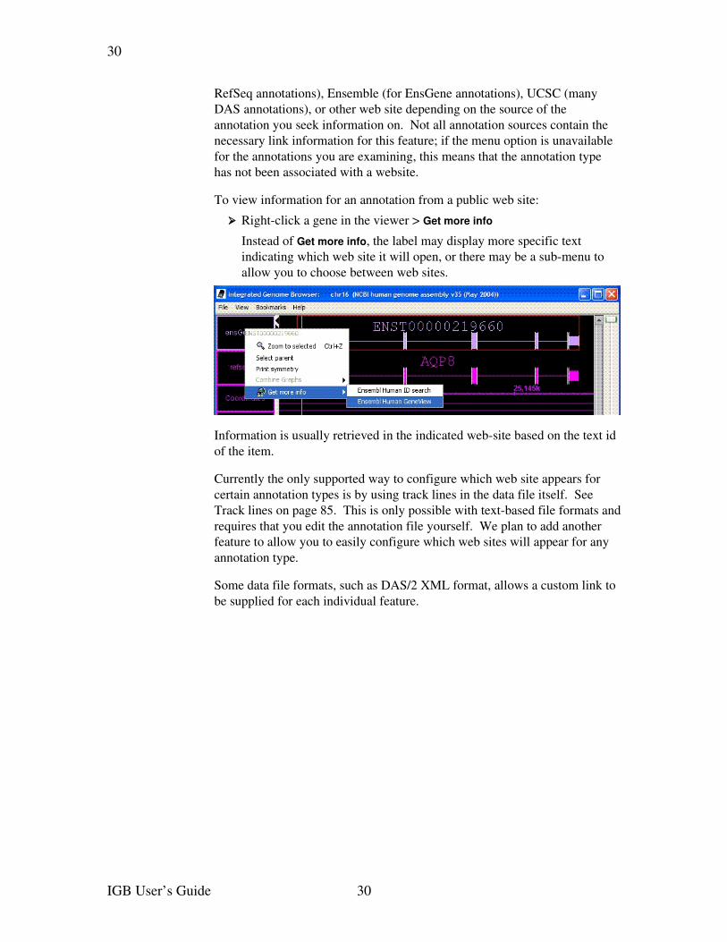
To view information for an annotation from a public web site:
➢ Rightclick a gene in the viewer > Get more info
Instead of Get more info, the label may display more specific text indicating which web site it will open, or there may be a submenu to allow you to choose between web sites.
Information is usually retrieved in the indicated website based on the text id of the item.
Currently the only supported way to configure which web site appears for certain annotation types is by using track lines in the data file itself. See Track lines on page 85. This is only possible with textbased file formats and requires that you edit the annotation file yourself. We plan to add another feature to allow you to easily configure which web sites will appear for any annotation type.
Some data file formats, such as DAS/2 XML format, allows a custom link to be supplied for each individual feature.
IGB User’s Guide 30
31
Working with sequence residues
Many IGB features require sequence residues to be loaded, so you may want to load them initially during each IGB session. However, sequence data can require a great deal of memory, so only load sequences if you need them.
Loading sequencesThere are three ways to load sequence residues into IGB. The first two of these are primarily for commonlystudied organisms.
➢ Load residues for a whole chromosome.
Click Data Access tab > Load all sequence
➢ Load residues for a small region. This is not always supported, in which case the full chromosome sequence will be loaded.
Click Data Access tab > Load sequence in view
➢ Load residues from a file.
Use File menu > Open File
➢ If data is not available on the configured servers for the selected sequence or chromosome, then an error message will appear. This error can also occur if you are viewing data from a genome that is not included in the configured servers.
➢ Wait while the sequences load. Sequence residues contain a large amount of data, so this may take a few minutes.
Some servers will reject requests for residues from a region that is too large. Others will return the data, but only after a very long wait.
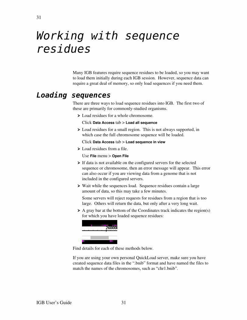
➢ A gray bar at the bottom of the Coordinates track indicates the region(s) for which you have loaded sequence residues:
Find details for each of these methods below.
If you are using your own personal QuickLoad server, make sure you have created sequence data files in the “.bnib” format and have named the files to match the names of the chromosomes, such as “chr1.bnib”.
IGB User’s Guide 31
32
Loading from a fileYou may choose to load sequence data for whole chromosomes, or even for whole genomes, from a file. The FASTA format can be used, but is only appropriate for small sequences. The filename should end with “.fasta” or “.fa”.
The FASTA format is described here: http://en.wikipedia.org/wiki/Fasta_format
Sequence files contain sequence residues only. If an annotation file you use lacks sequence residues, you can merge a sequence file for the same region.
To load a sequence file:
➢ Choose File menu > Open File.
➢ Navigate to the correct directory and select a file in FASTA format. The filename must end with “.fasta” or “.fa”.
➢ Choose whether you want to merge this with your current data:
➢ If you want to load one or more sequence(s) for the genome you are currently looking at, choose “Merge with currently loaded data”.
If the name(s) of the sequence(s) in the file match the names in your currentlyloaded genome, they will be merged into those chromosomes. Otherwise, new chromosomes will be added to your genome to hold the new data.
The number of residues should match the length of your loaded sequences. If not, then the sequence lengths will be increased as needed.
➢ If you want to create a new genome using the chromosome(s) or sequence(s) specified in the file, select “Create new genome”.
A new genome will be created containing sequence data from the file. There will be no annotation data associated with this genome, but you can load any annotations and graphs you have created in other files.
The FASTA format is good for small sequences. For larger sequences, you should convert your files to a more efficient binary format
The public QuickLoad server maintained by Affymetrix provides some sequence data in a binary format called “.bnib”. This file format is much more efficient and is preferred for large sequences, such as whole chromosomes.
Users interested in creating their own “.bnib” files should read this document: http://sourceforge.net/docman/display_doc.php?docid=27770&group_id=129420
IGB User’s Guide 32
33
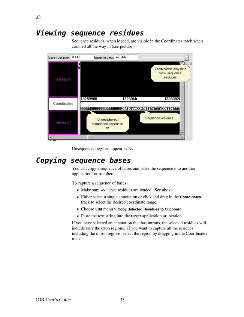
Viewing sequence residuesSequence residues, when loaded, are visible in the Coordinates track when zoomed all the way in (see picture).
Unsequenced regions appear as Ns.
Copying sequence basesYou can copy a sequence of bases and paste the sequence into another application for use there.
To capture a sequence of bases:
➢ Make sure sequence residues are loaded. See above.
➢ Either select a single annotation or click and drag in the Coordinates track to select the desired coordinate range.
➢ Choose Edit menu > Copy Selected Residues to Clipboard.
➢ Paste the text string into the target application or location.
If you have selected an annotation that has introns, the selected residues will include only the exon regions. If you want to capture all the residues including the intron regions, select the region by dragging in the Coordinates track.
IGB User’s Guide 33
34
Searching
Data sets from different genomes are kept distinct in memory. The search functions described below will search for data only in the current genome or chromosome, as noted below. You can switch between the different genomes and chromosomes by using the pulldown genome selector and table of chromosomes in the Data Access tab panel.
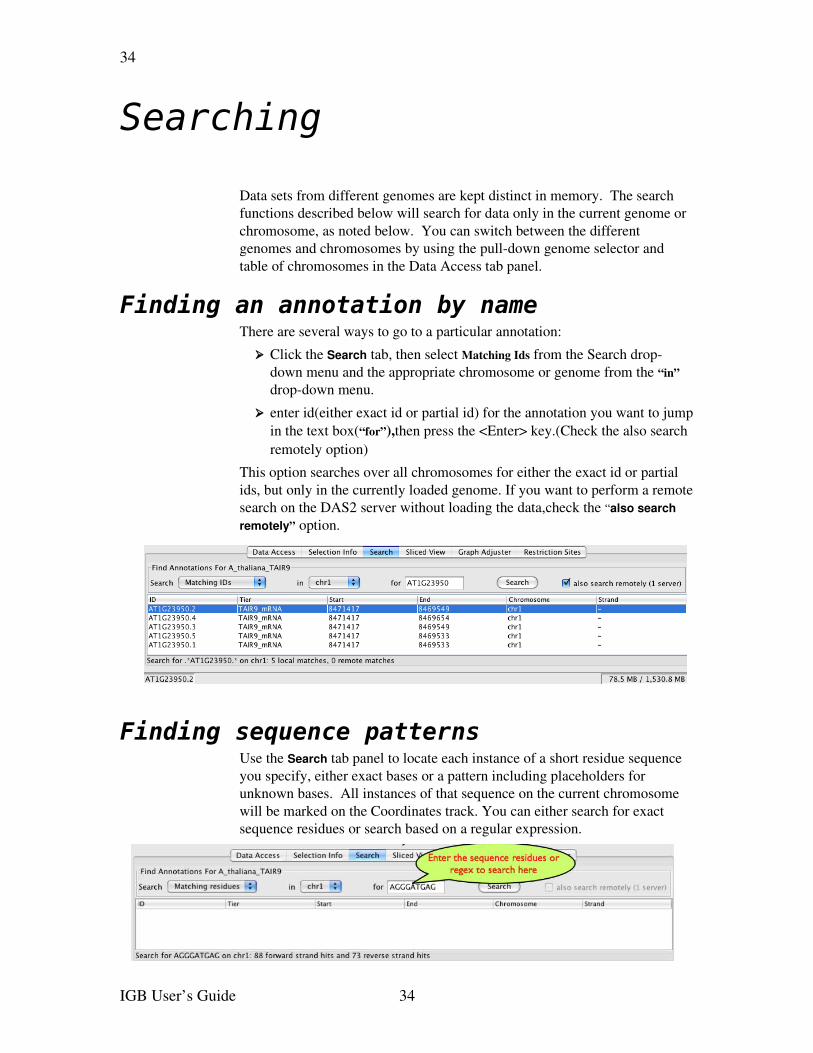
Finding an annotation by nameThere are several ways to go to a particular annotation:
➢ Click the Search tab, then select Matching Ids from the Search dropdown menu and the appropriate chromosome or genome from the “in” dropdown menu.
➢ enter id(either exact id or partial id) for the annotation you want to jump in the text box(“for”),then press the <Enter> key.(Check the also search remotely option)
This option searches over all chromosomes for either the exact id or partial ids, but only in the currently loaded genome. If you want to perform a remote search on the DAS2 server without loading the data,check the “also search remotely” option.
Finding sequence patternsUse the Search tab panel to locate each instance of a short residue sequence you specify, either exact bases or a pattern including placeholders for unknown bases. All instances of that sequence on the current chromosome will be marked on the Coordinates track. You can either search for exact sequence residues or search based on a regular expression.
IGB User’s Guide 34
35
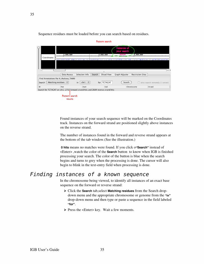
Sequence residues must be loaded before you can search based on residues.
Found instances of your search sequence will be marked on the Coordinates track. Instances on the forward strand are positioned slightly above instances on the reverse strand.
The number of instances found in the forward and reverse strand appears at the bottom of the tab window.(See the illustration.)
0 hits means no matches were found. If you click o“Search” instead of <Enter> ,watch the color of the Search button to know when IGB is finished processing your search. The color of the button is blue when the search begins and turns to grey when the processing is done. The cursor will also begin to blink in the textentry field when processing is done.
Finding instances of a known sequenceIn the chromosome being viewed, to identify all instances of an exact base sequence on the forward or reverse strand:
➢ Click the Search tab,select Matching residues from the Search dropdown menu and the appropriate chromosome or genome from the “in” dropdown menu and then type or paste a sequence in the field labeled “for”.
➢ Press the <Enter> key. Wait a few moments.
IGB User’s Guide 35
36
Finding instances of a sequence containing unknowns
In the chromosome being viewed, identify all sequences on the forward strand matching a regular expression (a sequence containing “wild card” nucleotides).
This search is casesensitive and limited to the forward strand for efficiency. FASTA files may contain both uppercase and lowercase sequences (lowercase is typically used for repeating sequences). If you are working with data with both upper and lower case residues, search for upper and lower case separately as desired. Or make the search be caseinsensitive by using the flag “(?i)” at the beginning of the regular expression.
➢ Click the Search tab and enter a casesensitive string of bases and wild cards (see table below for common ones) in the field labeled “for”.
➢ Press the <Enter> key. Wait a few moments; this may take some time.
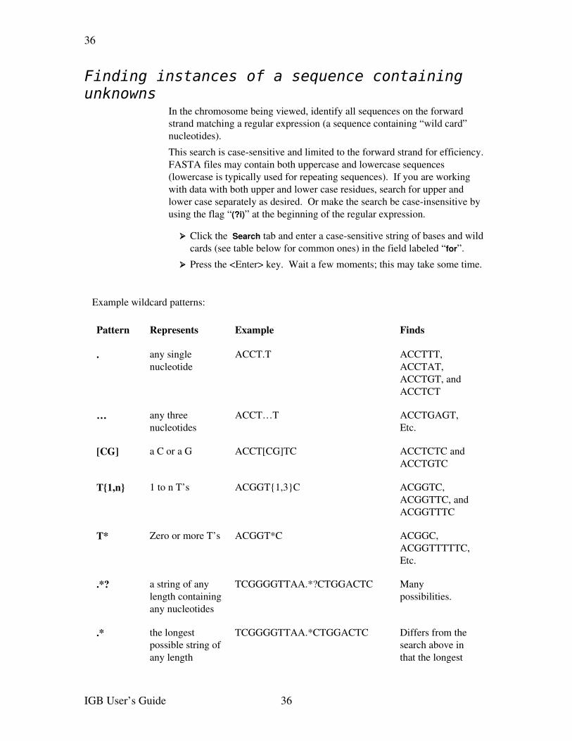
Example wildcard patterns:
Pattern Represents Example Finds
. any single nucleotide
ACCT.T ACCTTT, ACCTAT, ACCTGT, and ACCTCT
… any three nucleotides
ACCT…T ACCTGAGT, Etc.
[CG] a C or a G ACCT[CG]TC ACCTCTC and ACCTGTC
T{1,n} 1 to n T’s ACGGT{1,3}C ACGGTC, ACGGTTC, and ACGGTTTC
T* Zero or more T’s ACGGT*C ACGGC, ACGGTTTTTC, Etc.
.*? a string of any length containing any nucleotides
TCGGGGTTAA.*?CTGGACTC Many possibilities.
.* the longest possible string of any length
TCGGGGTTAA.*CTGGACTC Differs from the search above in that the longest
IGB User’s Guide 36

37
containing any nucleotides
possible result(s) will be found
(?i) use caseinsensitive matching
(?i)A[CG]T ACT, agt, acT, AGt, etc.
The full list of regular expression syntax that you can use in IGB is available at http://java.sun.com/j2se/1.5.0/docs/api/java/util/regex/Pattern.html
For more detailed information about wildcard searches in general, look for a book on the subject of “Regular Expressions”.
IGB User’s Guide 37
38
Customizing annotation tracks
Each annotation type that you load appears in its own annotation track. You can facilitate viewing and comparison by customizing the appearance of each annotation type and by adjusting the position and size of tracks relative to each other.
You can manipulate tracks in the ways described in the following sections. Many of these changes can also be made by opening the tier preferences panel with File > Preferences > Tiers panel. The effect is the same whichever method you use. Most of the changes will be remembered between sessions with IGB.
All annotation tracks have a track handle in the panel to the left of the viewer. For some annotation tracks, id labels will be displayed above or below each transcript. See Using annotation id labels below.
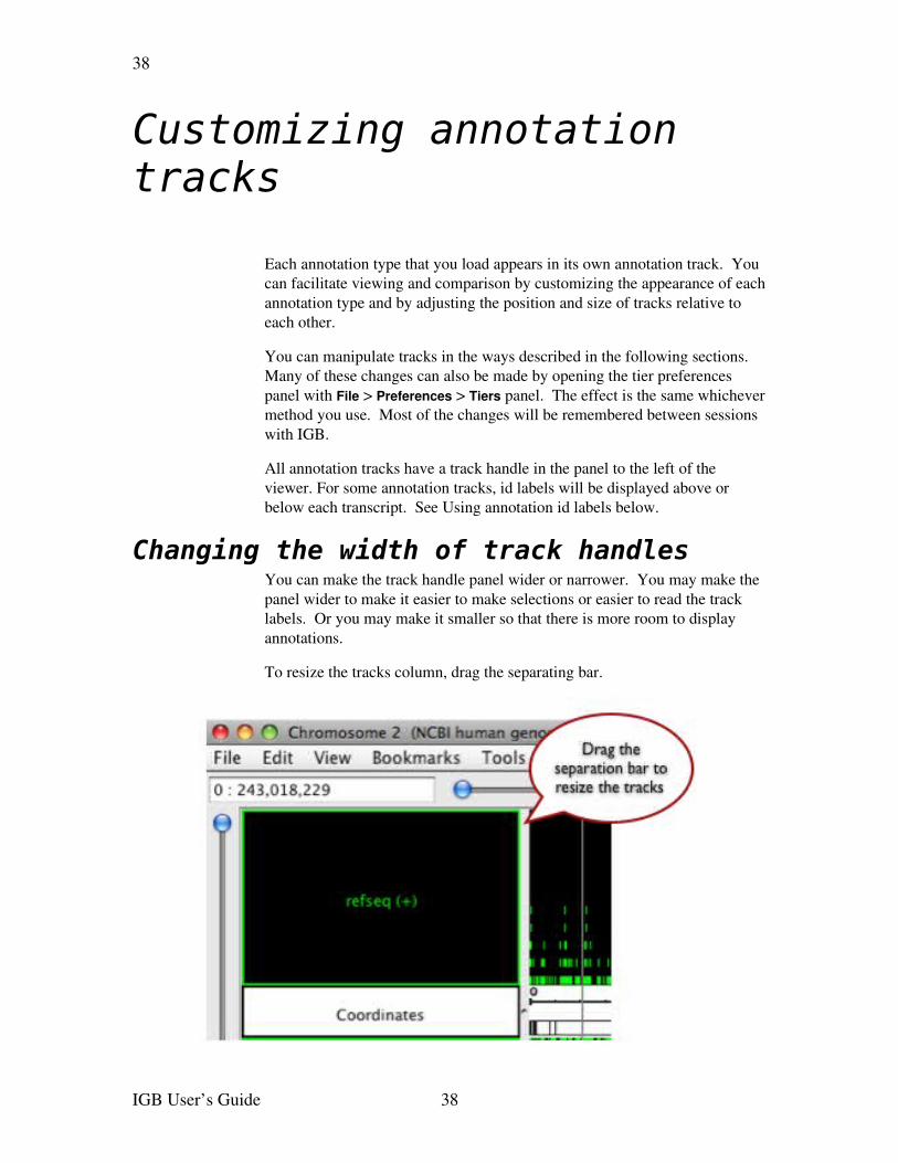
Changing the width of track handlesYou can make the track handle panel wider or narrower. You may make the panel wider to make it easier to make selections or easier to read the track labels. Or you may make it smaller so that there is more room to display annotations.
To resize the tracks column, drag the separating bar.
IGB User’s Guide 38
39
Re-ordering tracks top-to-bottom To reorder the tracks:
➢ Click a track name (in the panel on the left) and drag the track up or down to the desired location.
There is nothing preventing you from placing forward and reverse strand data either above or below the axis, at your choice.
Selecting tracksBefore changing any track properties, you will first need to select one or more tracks.
➢ Select a single track by clicking on its label.
➢ Select multiple tracks by shiftclicking.
➢ Select all tracks by Rightclick on track name > Select All Tiers
To perform rightclick operations on all the selected tracks simultaneously, rightclick one of the selected tracks to display the menu of track options.
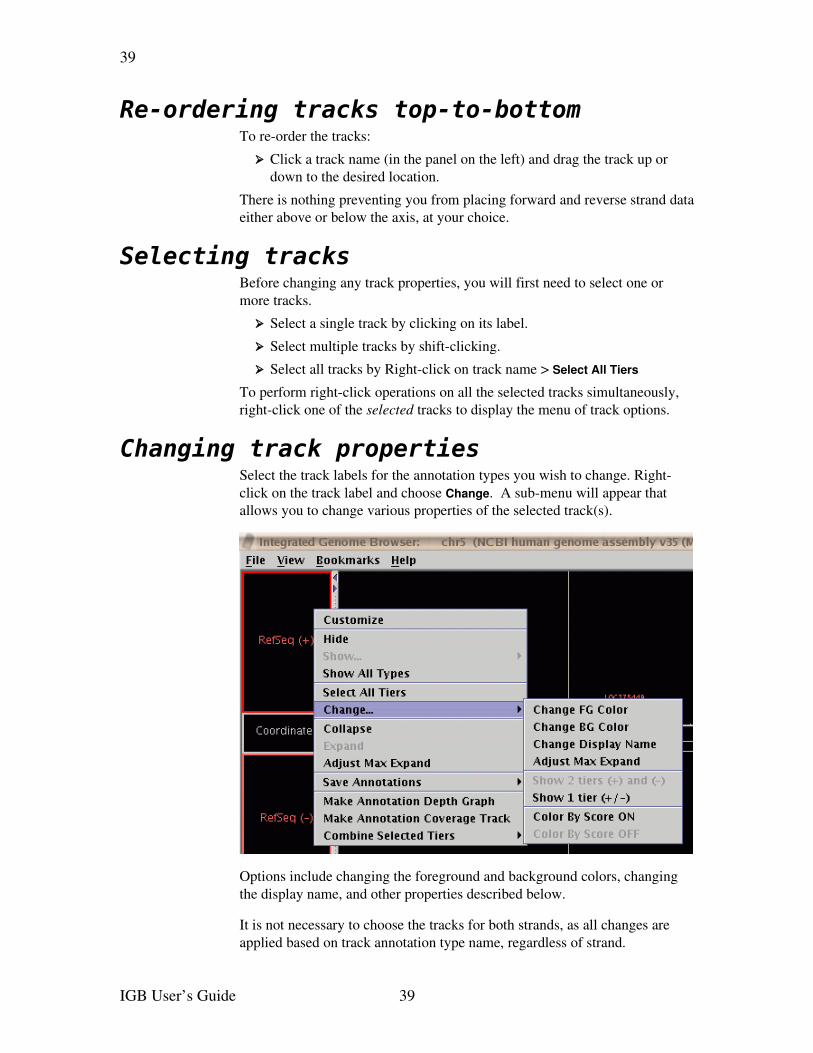
Changing track propertiesSelect the track labels for the annotation types you wish to change. Rightclick on the track label and choose Change. A submenu will appear that allows you to change various properties of the selected track(s).
Options include changing the foreground and background colors, changing the display name, and other properties described below.
It is not necessary to choose the tracks for both strands, as all changes are applied based on track annotation type name, regardless of strand.
IGB User’s Guide 39
40
You can also change these track properties by choosing the Customize menu item from the popup menu or from File menu > Preferences. The results are the same regardless of the method you use.
Changing annotation colorsTo change the color of annotations in a track:
➢ Rightclick the track name and choose Change > Change FG Color.
➢ Click a color in the palette, then click OK.
Change the background color in a similar manner. These changes will remain after you close and relaunch IGB and load the same data set.
Changing track namesSometimes you will want to change the displayed names of tracks because the default names are too long or are confusing to you.
To change the display name of annotations in a track:
➢ Rightclick the track name and choose Change > Change Display Name.
➢ Type the new name, then click OK.
Hiding and showing annotation tracksTracks can’t be deleted, but they can be hidden. To hide one or more selected annotation types:
➢ Rightclick on the track or tracks you want to hide > Hide
All strands of the selected annotation track will be hidden.
To show hidden tracks:
➢ Rightclick on a track label
➢ Select either Show All Types or Show > Track Name.
All strands of the selected annotation track will be shown, subject to your global choice of which strands to show. See the next section.
Hiding and showing strandsBy default, all strands of data are shown. Annotations on the forward (+) and reverse () strands can be shown in separate tracks, or in the same mixed strand (+/) track. Data with no known strand information is also indicated as a mixed strand (+/) track. Forward strands typically show above the axis and reverse strands typically show below the axis, but at this time there is nothing preventing you from rearranging the tiers so that this is not true.
You can control whether individual annotation types display as a single strand or as two separate strands. You can furthermore globally control which of these strand types are visible. These two functions interact to precisely limit the information shown to that which you are interested in.
IGB User’s Guide 40
41
To change the strands shown for each individual annotation type
➢ Select one or more track labels
➢ Rightclick on a track label > Change
➢ Select either Show as single tier or Show as two tiers
To change the strands shown for all annotation types
➢ Choose View menu > Strands
➢ Select any of these to toggle the selection on or off➢ Show (+) Tiers
➢ Show () Tiers
➢ Show (+/) Tiers
Note how these two functions interact with each other and with the hiding and showing of annotation types:
➢ Hiding the reverse () tiers will only hide tiers that contain only reversestrand annotations. It will NOT hide the reversestrand annotations in mixedstrand (+/) tiers.
➢ If you have hidden an annotation type (such as RefSeq) and then choose to show it again, which tiers are visible will still be subject to your selections of which strands to display.
Collapsing and expanding tracksFor tracks containing multiple rows of annotations, collapsing tracks consolidates all rows within a track into a single row. Annotations on any of the rows will be included in the collapsed track.
Collapsing tracks is useful if you don't need to see all the details. But be aware that in collapsed tracks larger annotations may obscure smaller ones; annotations with introns may be obscured by annotations that don’t show the intron.
To collapse or expand selected tracks:
➢ Rightclick on a track label > Collapse or Expand
All strands of the given annotation type will be affected.
IGB User’s Guide 41
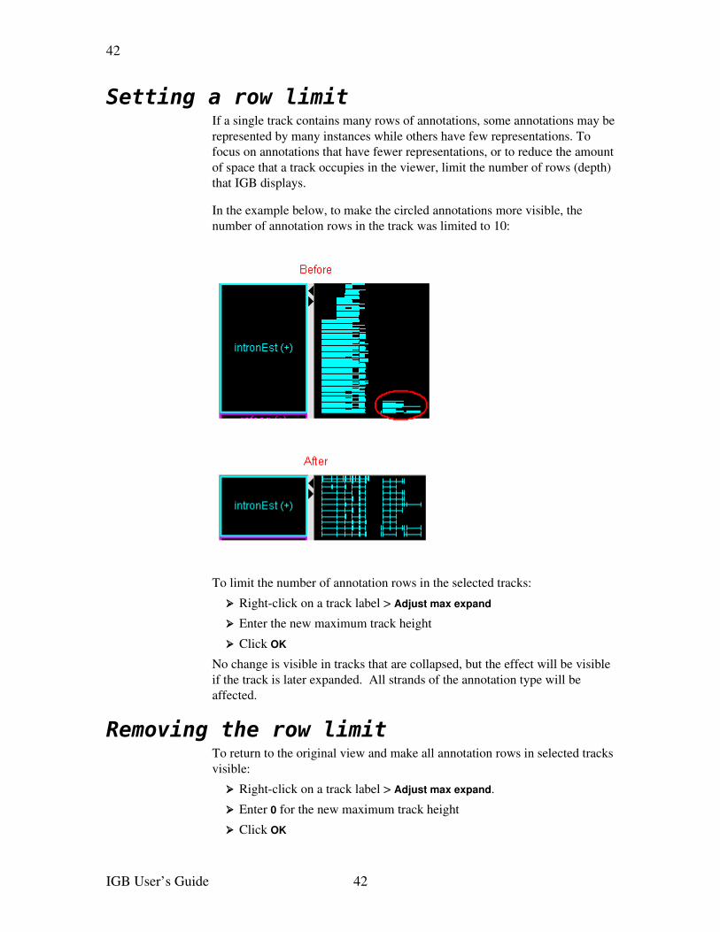
42
Setting a row limit If a single track contains many rows of annotations, some annotations may be represented by many instances while others have few representations. To focus on annotations that have fewer representations, or to reduce the amount of space that a track occupies in the viewer, limit the number of rows (depth) that IGB displays.
In the example below, to make the circled annotations more visible, the number of annotation rows in the track was limited to 10:
To limit the number of annotation rows in the selected tracks:
➢ Rightclick on a track label > Adjust max expand
➢ Enter the new maximum track height
➢ Click OK
No change is visible in tracks that are collapsed, but the effect will be visible if the track is later expanded. All strands of the annotation type will be affected.
Removing the row limitTo return to the original view and make all annotation rows in selected tracks visible:
➢ Rightclick on a track label > Adjust max expand.
➢ Enter 0 for the new maximum track height
➢ Click OK
IGB User’s Guide 42
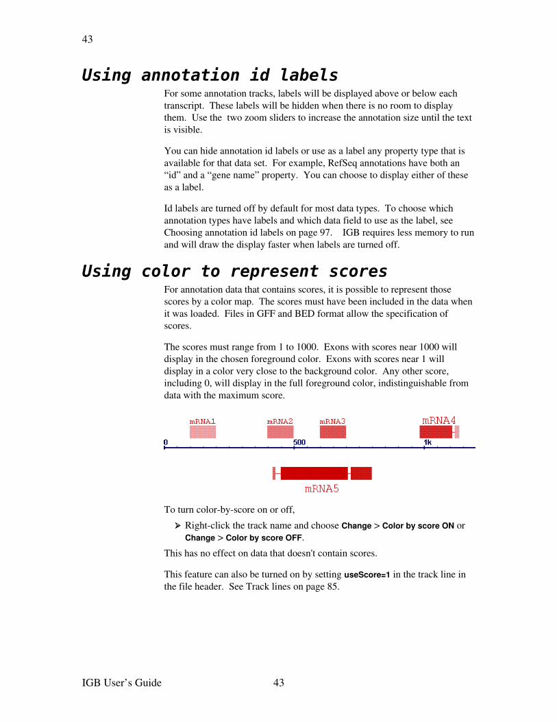
43
Using annotation id labelsFor some annotation tracks, labels will be displayed above or below each transcript. These labels will be hidden when there is no room to display them. Use the two zoom sliders to increase the annotation size until the text is visible.
You can hide annotation id labels or use as a label any property type that is available for that data set. For example, RefSeq annotations have both an “id” and a “gene name” property. You can choose to display either of these as a label.
Id labels are turned off by default for most data types. To choose which annotation types have labels and which data field to use as the label, see Choosing annotation id labels on page 97. IGB requires less memory to run and will draw the display faster when labels are turned off.
Using color to represent scoresFor annotation data that contains scores, it is possible to represent those scores by a color map. The scores must have been included in the data when it was loaded. Files in GFF and BED format allow the specification of scores.
The scores must range from 1 to 1000. Exons with scores near 1000 will display in the chosen foreground color. Exons with scores near 1 will display in a color very close to the background color. Any other score, including 0, will display in the full foreground color, indistinguishable from data with the maximum score.
To turn colorbyscore on or off,
➢ Rightclick the track name and choose Change > Color by score ON or Change > Color by score OFF.
This has no effect on data that doesn't contain scores.
This feature can also be turned on by setting useScore=1 in the track line in the file header. See Track lines on page 85.
IGB User’s Guide 43
44
Tools for comparing annotations
IGB offers several tools to highlight patterns to aid in making comparisons. These are described in the following sections.
Highlighting matching endpointsTo see if different data sources show the same start and endpoints for an annotation:
➢ Select an item.
Matching edges of corresponding items in all tracks being viewed will be highlighted
➢ By default, the highlight color is white, which works well on a black background. If you change the background color, you may want to change the edgematching color as well.
Use View menu > Adjust edge match fuzziness > Edge Sensitivity Adjuster dialog box > Edge match colors > Standard.
To specify the degree of closeness required for a match (how many base pairs difference is still considered a match):
➢ Choose View menu > Adjust edge match fuzziness.
➢ Slide the slider to the maximum number of base pairs difference that you want to consider a match.
By default, if edge match fuzziness is adjusted, all matching edges are highlighted in gray rather than in white. This color can also be changed using View menu > Adjust edge match fuzziness > Edge Sensitivity Adjuster dialog box > Edge match colors > Fuzzy matching.
SlicingSlicing makes slight variations more visible when comparing multiple annotations on the same sequence. Slicing cuts out long introns and realigns the exons of a selected annotation or set of annotations, making pattern irregularities and possible alternate splicing more obvious.
IGB User’s Guide 44
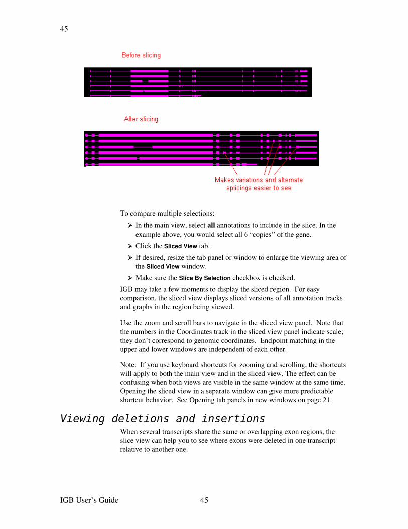
45
To compare multiple selections:
➢ In the main view, select all annotations to include in the slice. In the example above, you would select all 6 “copies” of the gene.
➢ Click the Sliced View tab.
➢ If desired, resize the tab panel or window to enlarge the viewing area of the Sliced View window.
➢ Make sure the Slice By Selection checkbox is checked.
IGB may take a few moments to display the sliced region. For easy comparison, the sliced view displays sliced versions of all annotation tracks and graphs in the region being viewed.
Use the zoom and scroll bars to navigate in the sliced view panel. Note that the numbers in the Coordinates track in the sliced view panel indicate scale; they don’t correspond to genomic coordinates. Endpoint matching in the upper and lower windows are independent of each other.
Note: If you use keyboard shortcuts for zooming and scrolling, the shortcuts will apply to both the main view and in the sliced view. The effect can be confusing when both views are visible in the same window at the same time. Opening the sliced view in a separate window can give more predictable shortcut behavior. See Opening tab panels in new windows on page 21.
Viewing deletions and insertionsWhen several transcripts share the same or overlapping exon regions, the slice view can help you to see where exons were deleted in one transcript relative to another one.
IGB User’s Guide 45
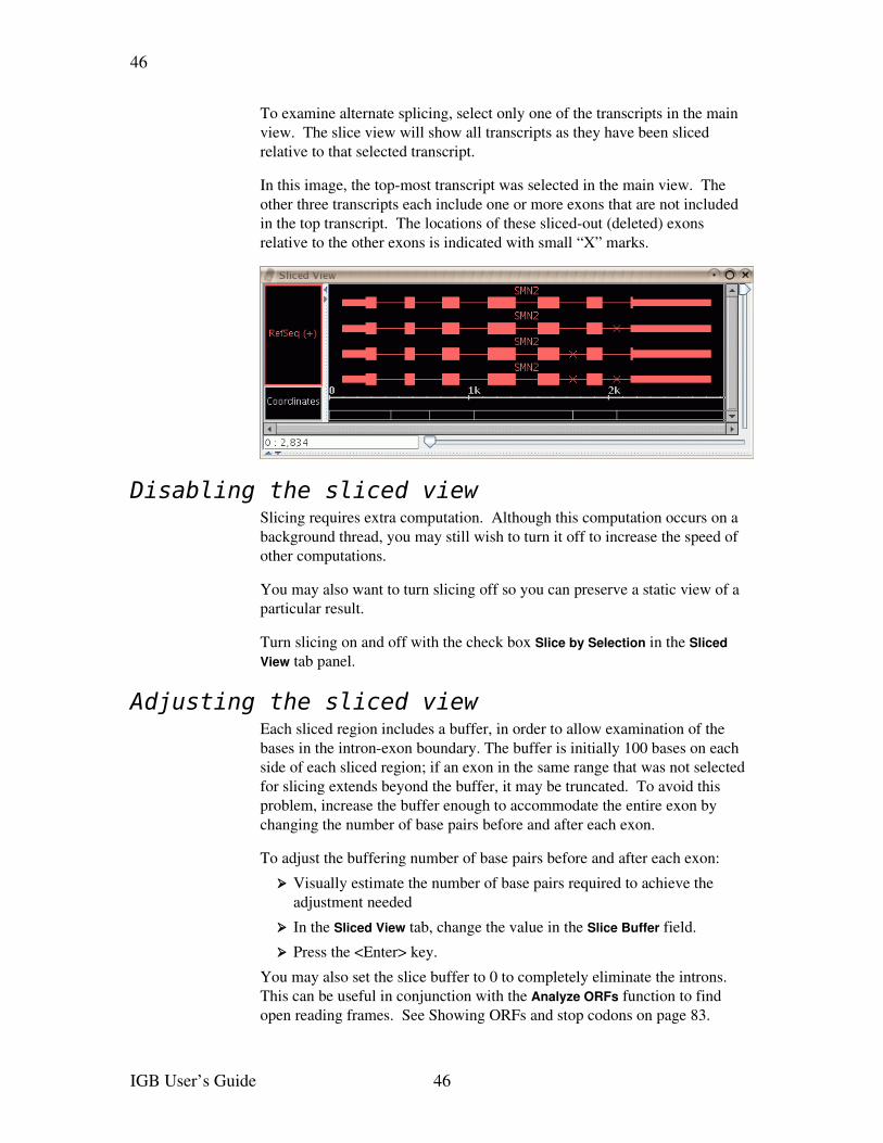
46
To examine alternate splicing, select only one of the transcripts in the main view. The slice view will show all transcripts as they have been sliced relative to that selected transcript.
In this image, the topmost transcript was selected in the main view. The other three transcripts each include one or more exons that are not included in the top transcript. The locations of these slicedout (deleted) exons relative to the other exons is indicated with small “X” marks.
Disabling the sliced viewSlicing requires extra computation. Although this computation occurs on a background thread, you may still wish to turn it off to increase the speed of other computations.
You may also want to turn slicing off so you can preserve a static view of a particular result.
Turn slicing on and off with the check box Slice by Selection in the Sliced View tab panel.
Adjusting the sliced viewEach sliced region includes a buffer, in order to allow examination of the bases in the intronexon boundary. The buffer is initially 100 bases on each side of each sliced region; if an exon in the same range that was not selected for slicing extends beyond the buffer, it may be truncated. To avoid this problem, increase the buffer enough to accommodate the entire exon by changing the number of base pairs before and after each exon.
To adjust the buffering number of base pairs before and after each exon:
➢ Visually estimate the number of base pairs required to achieve the adjustment needed
➢ In the Sliced View tab, change the value in the Slice Buffer field.
➢ Press the <Enter> key.
You may also set the slice buffer to 0 to completely eliminate the introns. This can be useful in conjunction with the Analyze ORFs function to find open reading frames. See Showing ORFs and stop codons on page 83.
IGB User’s Guide 46
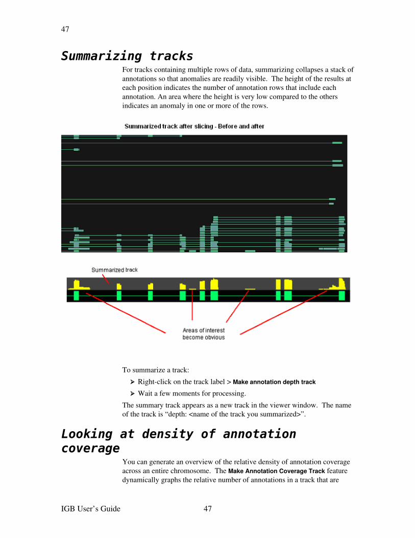
47
Summarizing tracksFor tracks containing multiple rows of data, summarizing collapses a stack of annotations so that anomalies are readily visible. The height of the results at each position indicates the number of annotation rows that include each annotation. An area where the height is very low compared to the others indicates an anomaly in one or more of the rows.
To summarize a track:
➢ Rightclick on the track label > Make annotation depth track
➢ Wait a few moments for processing.
The summary track appears as a new track in the viewer window. The name of the track is “depth: <name of the track you summarized>”.
Looking at density of annotation coverage
You can generate an overview of the relative density of annotation coverage across an entire chromosome. The Make Annotation Coverage Track feature dynamically graphs the relative number of annotations in a track that are
IGB User’s Guide 47
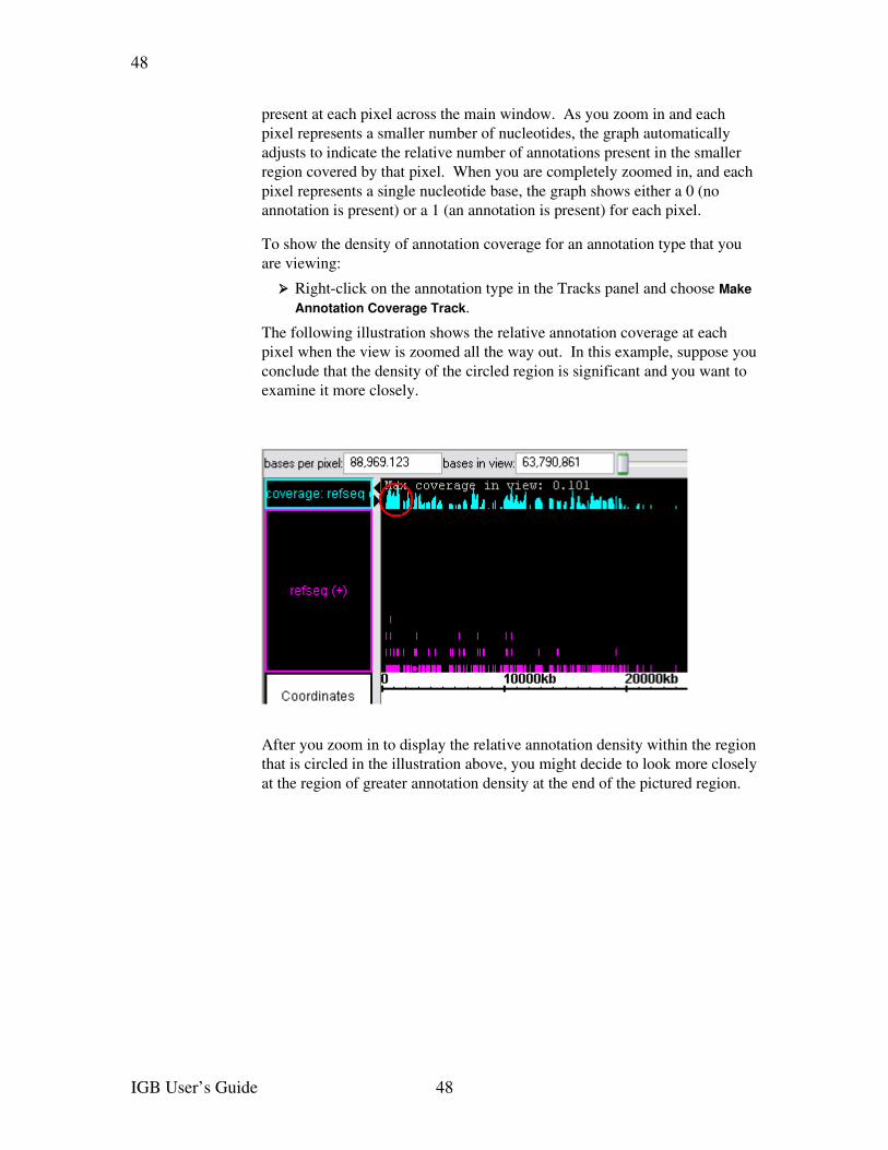
48
present at each pixel across the main window. As you zoom in and each pixel represents a smaller number of nucleotides, the graph automatically adjusts to indicate the relative number of annotations present in the smaller region covered by that pixel. When you are completely zoomed in, and each pixel represents a single nucleotide base, the graph shows either a 0 (no annotation is present) or a 1 (an annotation is present) for each pixel.
To show the density of annotation coverage for an annotation type that you are viewing:
➢ Rightclick on the annotation type in the Tracks panel and choose Make Annotation Coverage Track.
The following illustration shows the relative annotation coverage at each pixel when the view is zoomed all the way out. In this example, suppose you conclude that the density of the circled region is significant and you want to examine it more closely.
After you zoom in to display the relative annotation density within the region that is circled in the illustration above, you might decide to look more closely at the region of greater annotation density at the end of the pictured region.
IGB User’s Guide 48
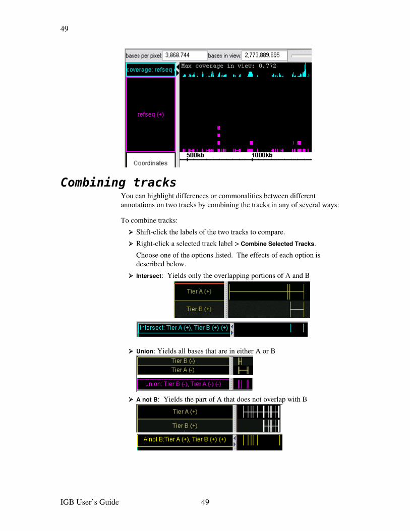
49
Combining tracksYou can highlight differences or commonalities between different annotations on two tracks by combining the tracks in any of several ways:
To combine tracks:
➢ Shiftclick the labels of the two tracks to compare.
➢ Rightclick a selected track label > Combine Selected Tracks.
Choose one of the options listed. The effects of each option is described below.
➢ Intersect: Yields only the overlapping portions of A and B
➢ Union: Yields all bases that are in either A or B
➢ A not B: Yields the part of A that does not overlap with B
IGB User’s Guide 49
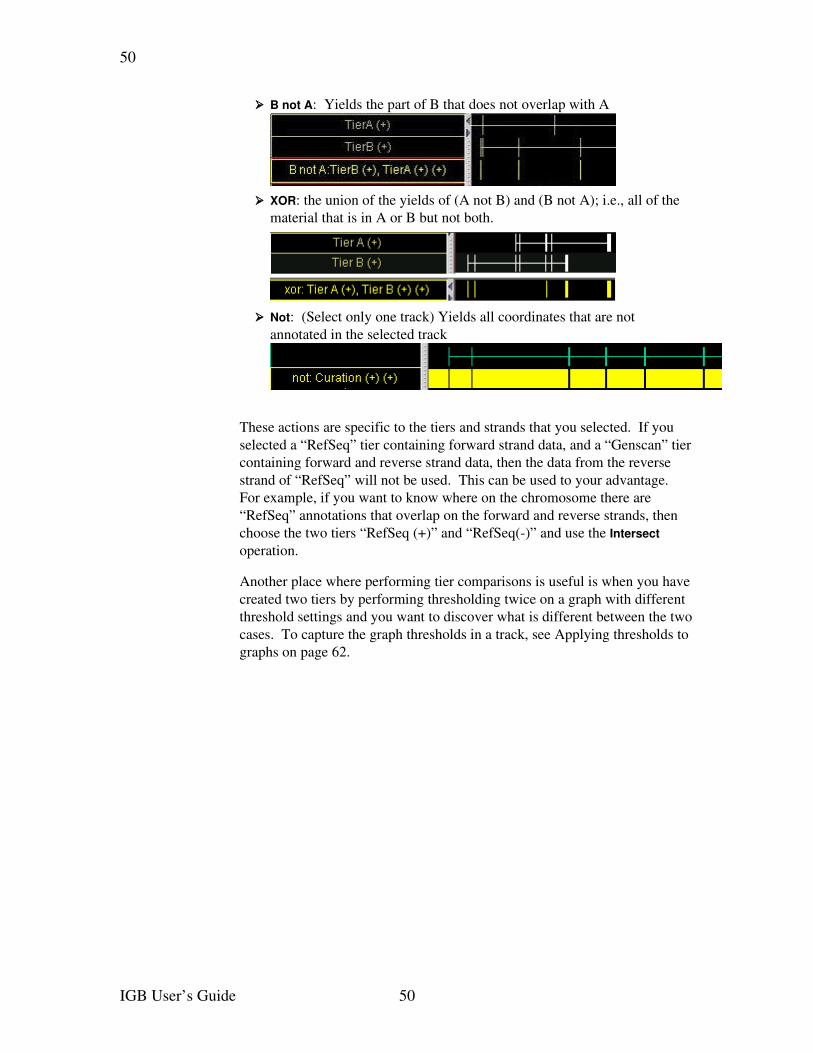
50
➢ B not A: Yields the part of B that does not overlap with A
➢ XOR: the union of the yields of (A not B) and (B not A); i.e., all of the material that is in A or B but not both.
➢ Not: (Select only one track) Yields all coordinates that are not annotated in the selected track
These actions are specific to the tiers and strands that you selected. If you selected a “RefSeq” tier containing forward strand data, and a “Genscan” tier containing forward and reverse strand data, then the data from the reverse strand of “RefSeq” will not be used. This can be used to your advantage. For example, if you want to know where on the chromosome there are “RefSeq” annotations that overlap on the forward and reverse strands, then choose the two tiers “RefSeq (+)” and “RefSeq()” and use the Intersect operation.
Another place where performing tier comparisons is useful is when you have created two tiers by performing thresholding twice on a graph with different threshold settings and you want to discover what is different between the two cases. To capture the graph thresholds in a track, see Applying thresholds tographs on page 62.
IGB User’s Guide 50
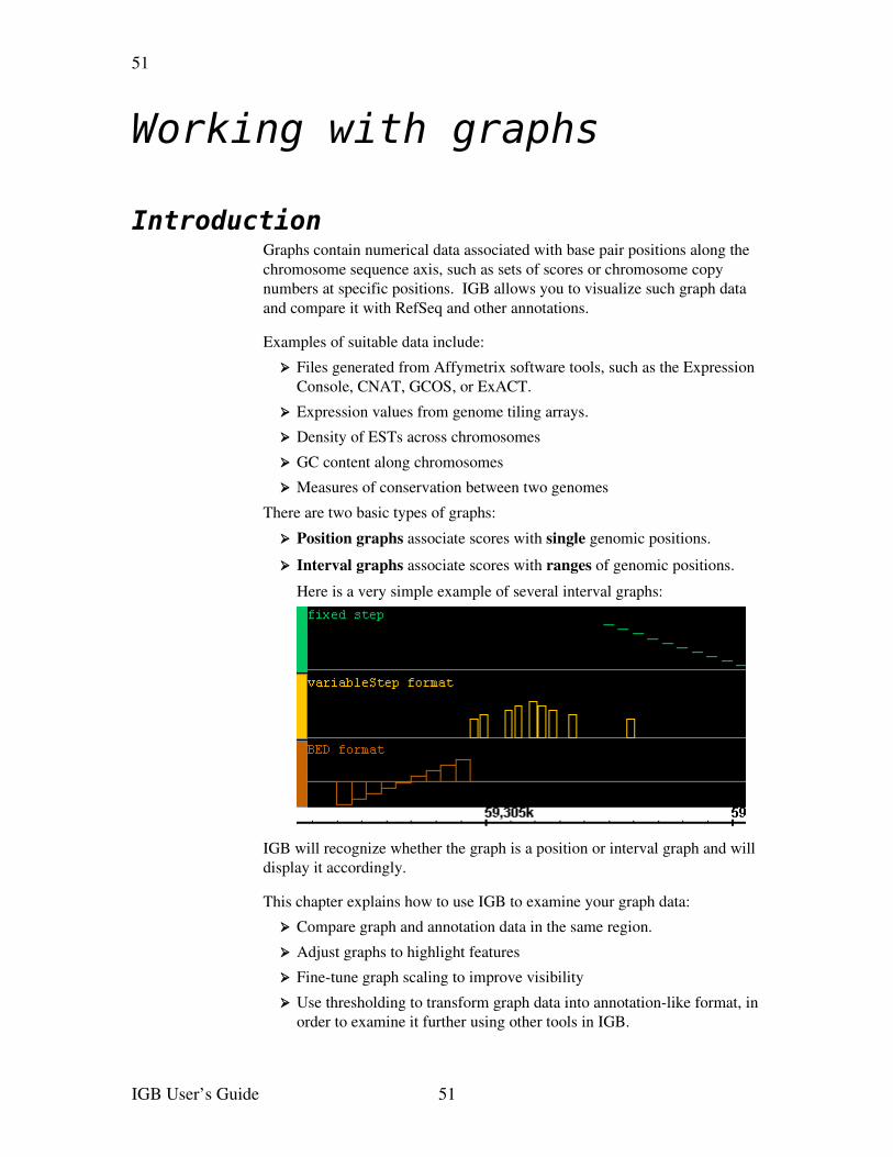
51
Working with graphs
IntroductionGraphs contain numerical data associated with base pair positions along the chromosome sequence axis, such as sets of scores or chromosome copy numbers at specific positions. IGB allows you to visualize such graph data and compare it with RefSeq and other annotations.
Examples of suitable data include:
➢ Files generated from Affymetrix software tools, such as the Expression Console, CNAT, GCOS, or ExACT.
➢ Expression values from genome tiling arrays.
➢ Density of ESTs across chromosomes
➢ GC content along chromosomes
➢ Measures of conservation between two genomes
There are two basic types of graphs:
➢ Position graphs associate scores with single genomic positions.
➢ Interval graphs associate scores with ranges of genomic positions.
Here is a very simple example of several interval graphs:
IGB will recognize whether the graph is a position or interval graph and will display it accordingly.
This chapter explains how to use IGB to examine your graph data:
➢ Compare graph and annotation data in the same region.
➢ Adjust graphs to highlight features
➢ Finetune graph scaling to improve visibility
➢ Use thresholding to transform graph data into annotationlike format, in order to examine it further using other tools in IGB.
IGB User’s Guide 51
52
Loading graph filesGraph files are loaded in the same way as annotation data files. To open graph files in any of the supported formats:
➢ Follow the procedures in Loading annotations from files on page 26.
IGB can display graphs in several file formats, developed at Affymetrix or elsewhere. For the most uptodate descriptions of the formats IGB supports, check the File menu > Open File, and look for documentation on the site http://genoviz.sourceforge.net/
All filenames must include the filename extension, for example “.sgr”. Compressed files must include the graph type extension AND the compression extension, such as “mygraph.sgr.zip”.
Graph files may be in the following formats:
.bar Generated from tiling arrays by TAS (Tiling Analysis Software.)
.chp Binary files generated by Affymetrix software. These files contain data on scores for probe sets. There are multiple variations on this file format. IGB can read some, but not all of these formats.
.egr Files containing data for scored intervals.
Files generated from Affymetrix GeneChip Operating Software (GCOS) or ExACT (Exon Array Computational Tool) software.
.sgr Sequence graph files that show base coordinate scores. These files are generated by CNAT (the Affymetrix Chromosome Copy Number Analysis Tool software).
The format of .sgr text files is: chromosome identification, then two columns of numbers separated by a single space or a tab. The first number is the base position; the second number is the score.
.gr A simple text format containing two columns of numbers separated by a single space or tab. The first number is the base position; the second number is the score.
Because this format does not include chromosome names, we recommend you use the “.sgr” format or “.wig” format instead.
.wig Wiggle format. A text format developed for use in the UCSC genome browser. All three subformats of wiggle graph are supported by IGB: “fixedStep”, “variableStep” and “BED”.
See http://genome.ucsc.edu/goldenPath/help/wiggle.html
Files in wiggle format can use UCSC track lines to specify colors and other properties. See Track lines on page 85.
IGB User’s Guide 52
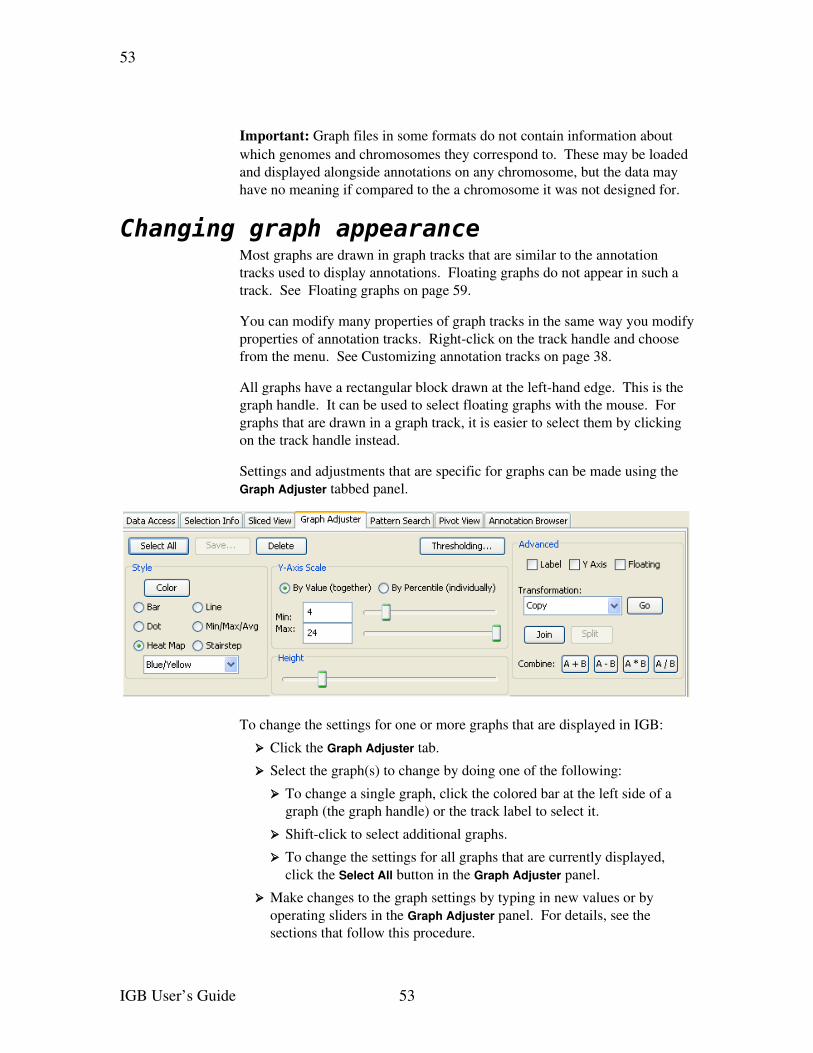
53
Important: Graph files in some formats do not contain information about which genomes and chromosomes they correspond to. These may be loaded and displayed alongside annotations on any chromosome, but the data may have no meaning if compared to the a chromosome it was not designed for.
Changing graph appearanceMost graphs are drawn in graph tracks that are similar to the annotation tracks used to display annotations. Floating graphs do not appear in such a track. See Floating graphs on page 59.
You can modify many properties of graph tracks in the same way you modify properties of annotation tracks. Rightclick on the track handle and choose from the menu. See Customizing annotation tracks on page 38.
All graphs have a rectangular block drawn at the lefthand edge. This is the graph handle. It can be used to select floating graphs with the mouse. For graphs that are drawn in a graph track, it is easier to select them by clicking on the track handle instead.
Settings and adjustments that are specific for graphs can be made using the Graph Adjuster tabbed panel.
To change the settings for one or more graphs that are displayed in IGB:
➢ Click the Graph Adjuster tab.
➢ Select the graph(s) to change by doing one of the following:
➢ To change a single graph, click the colored bar at the left side of a graph (the graph handle) or the track label to select it.
➢ Shiftclick to select additional graphs.
➢ To change the settings for all graphs that are currently displayed, click the Select All button in the Graph Adjuster panel.
➢ Make changes to the graph settings by typing in new values or by operating sliders in the Graph Adjuster panel. For details, see the sections that follow this procedure.
IGB User’s Guide 53
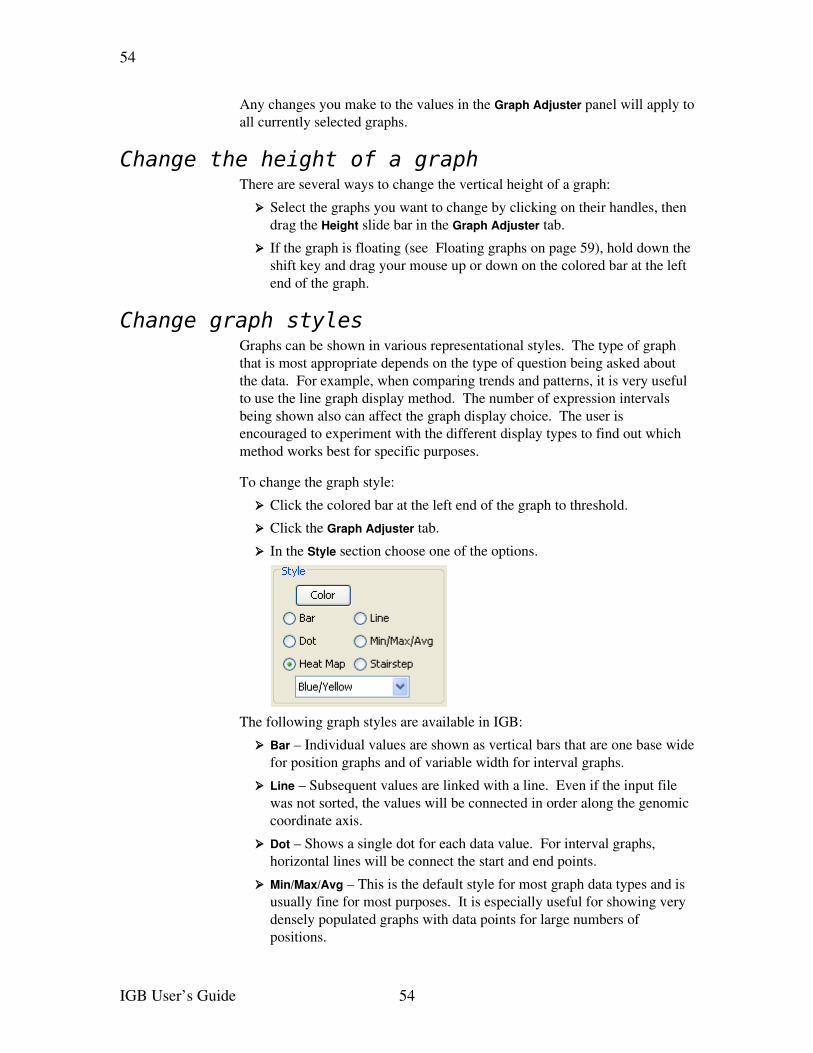
54
Any changes you make to the values in the Graph Adjuster panel will apply to all currently selected graphs.
Change the height of a graphThere are several ways to change the vertical height of a graph:
➢ Select the graphs you want to change by clicking on their handles, then drag the Height slide bar in the Graph Adjuster tab.
➢ If the graph is floating (see Floating graphs on page 59), hold down the shift key and drag your mouse up or down on the colored bar at the left end of the graph.
Change graph stylesGraphs can be shown in various representational styles. The type of graph that is most appropriate depends on the type of question being asked about the data. For example, when comparing trends and patterns, it is very useful to use the line graph display method. The number of expression intervals being shown also can affect the graph display choice. The user is encouraged to experiment with the different display types to find out which method works best for specific purposes.
To change the graph style:
➢ Click the colored bar at the left end of the graph to threshold.
➢ Click the Graph Adjuster tab.
➢ In the Style section choose one of the options.
The following graph styles are available in IGB:
➢ Bar – Individual values are shown as vertical bars that are one base wide for position graphs and of variable width for interval graphs.
➢ Line – Subsequent values are linked with a line. Even if the input file was not sorted, the values will be connected in order along the genomic coordinate axis.
➢ Dot – Shows a single dot for each data value. For interval graphs, horizontal lines will be connect the start and end points.
➢ Min/Max/Avg – This is the default style for most graph data types and is usually fine for most purposes. It is especially useful for showing very densely populated graphs with data points for large numbers of positions.
IGB User’s Guide 54

55
When IGB is zoomed all the way in, the display is equivalent to the Bar style. When zooming out, IGB starts to summarize values. When the scale of the display reaches the point where individual xvalues are associated with multiple score values, IGB picks the maximum and minimum values and draws a vertical bar between them. In addition, IBG draws lines through the average of all the data points represented at each x value.
➢ Stairstep – Similar to the bar graph style, except that bar widths along the horizontal axis are stairstepped.
For example, if position 100 has a value of 50 and position 200 has a value of 75 and there are no values in between, then IGB will draw a bar of height 50 that starts at position 100 and stops at position 200. Then, at position 200, IGB will draw a new bar of height 75 that terminates at the next location with a value.
This style is particularly useful for viewing .egr and .sgr files, ESTs, or other highdensity data.
➢ Heat map – Instead of showing relative intensity via the height of the line at each pixel or coordinate as in most other graph styles, a heat map shows expression levels via color or brightness of the line at each pixel or coordinate. This graph style is useful if you want areas of greater expression to jump out at you. If a graph does not render or is hard to see, adjust the visible bounds of the graph until features are readily visible. Several heat map color maps are available to choose from. Transparent color maps are available and may be useful for floating graphs.
The following image illustrates how a single data set would look in each of the graph styles. The graph used for this image is a simple position graph. An example of an interval graph was given in the introduction to this chapter.
IGB User’s Guide 55
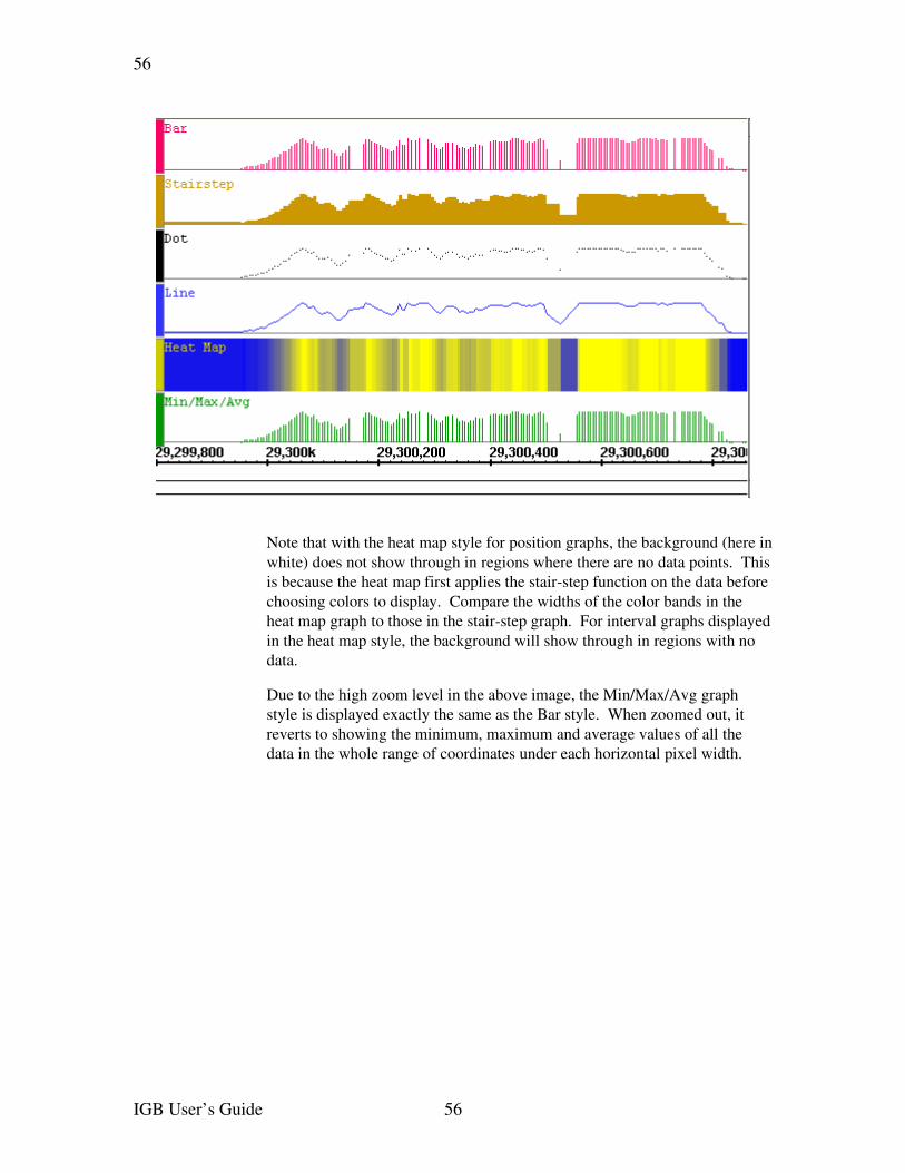
56
Note that with the heat map style for position graphs, the background (here in white) does not show through in regions where there are no data points. This is because the heat map first applies the stairstep function on the data before choosing colors to display. Compare the widths of the color bands in the heat map graph to those in the stairstep graph. For interval graphs displayed in the heat map style, the background will show through in regions with no data.
Due to the high zoom level in the above image, the Min/Max/Avg graph style is displayed exactly the same as the Bar style. When zoomed out, it reverts to showing the minimum, maximum and average values of all the data in the whole range of coordinates under each horizontal pixel width.
IGB User’s Guide 56
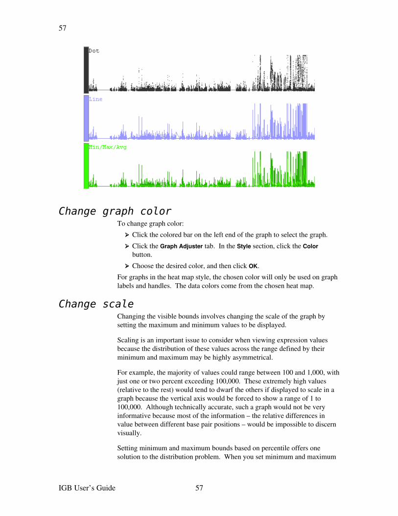
57
Change graph colorTo change graph color:
➢ Click the colored bar on the left end of the graph to select the graph.
➢ Click the Graph Adjuster tab. In the Style section, click the Color button.
➢ Choose the desired color, and then click OK.
For graphs in the heat map style, the chosen color will only be used on graph labels and handles. The data colors come from the chosen heat map.
Change scaleChanging the visible bounds involves changing the scale of the graph by setting the maximum and minimum values to be displayed.
Scaling is an important issue to consider when viewing expression values because the distribution of these values across the range defined by their minimum and maximum may be highly asymmetrical.
For example, the majority of values could range between 100 and 1,000, with just one or two percent exceeding 100,000. These extremely high values (relative to the rest) would tend to dwarf the others if displayed to scale in a graph because the vertical axis would be forced to show a range of 1 to 100,000. Although technically accurate, such a graph would not be very informative because most of the information – the relative differences in value between different base pair positions – would be impossible to discern visually.
Setting minimum and maximum bounds based on percentile offers one solution to the distribution problem. When you set minimum and maximum
IGB User’s Guide 57
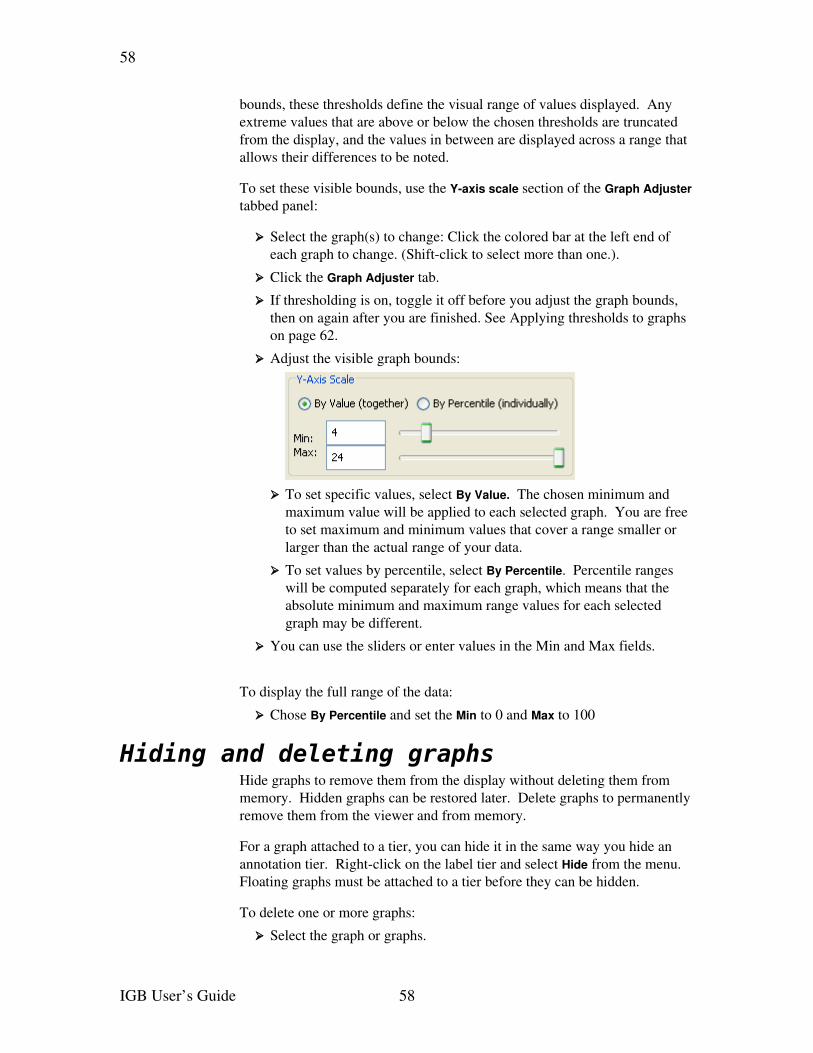
58
bounds, these thresholds define the visual range of values displayed. Any extreme values that are above or below the chosen thresholds are truncated from the display, and the values in between are displayed across a range that allows their differences to be noted.
To set these visible bounds, use the Yaxis scale section of the Graph Adjuster tabbed panel:
➢ Select the graph(s) to change: Click the colored bar at the left end of each graph to change. (Shiftclick to select more than one.).
➢ Click the Graph Adjuster tab.
➢ If thresholding is on, toggle it off before you adjust the graph bounds, then on again after you are finished. See Applying thresholds to graphs on page 62.
➢ Adjust the visible graph bounds:
➢ To set specific values, select By Value. The chosen minimum and maximum value will be applied to each selected graph. You are free to set maximum and minimum values that cover a range smaller or larger than the actual range of your data.
➢ To set values by percentile, select By Percentile. Percentile ranges will be computed separately for each graph, which means that the absolute minimum and maximum range values for each selected graph may be different.
➢ You can use the sliders or enter values in the Min and Max fields.
To display the full range of the data:
➢ Chose By Percentile and set the Min to 0 and Max to 100
Hiding and deleting graphsHide graphs to remove them from the display without deleting them from memory. Hidden graphs can be restored later. Delete graphs to permanently remove them from the viewer and from memory.
For a graph attached to a tier, you can hide it in the same way you hide an annotation tier. Rightclick on the label tier and select Hide from the menu. Floating graphs must be attached to a tier before they can be hidden.
To delete one or more graphs:
➢ Select the graph or graphs.
IGB User’s Guide 58
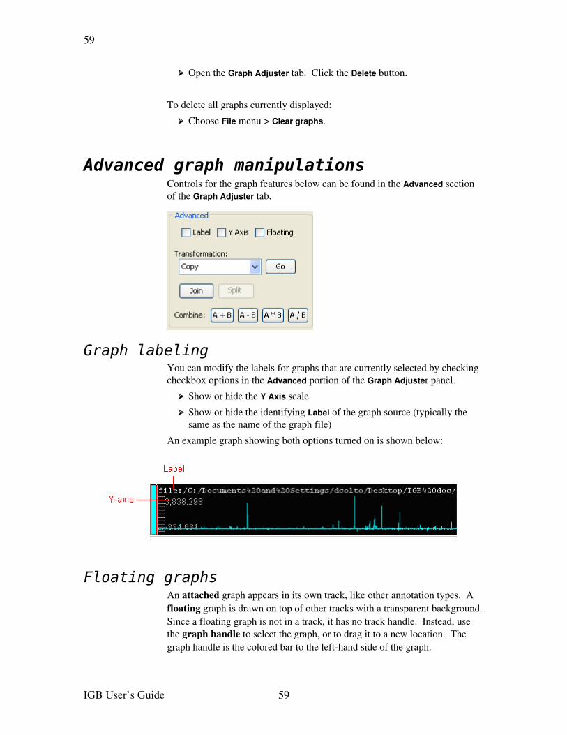
59
➢ Open the Graph Adjuster tab. Click the Delete button.
To delete all graphs currently displayed:
➢ Choose File menu > Clear graphs.
Advanced graph manipulationsControls for the graph features below can be found in the Advanced section of the Graph Adjuster tab.
Graph labelingYou can modify the labels for graphs that are currently selected by checking checkbox options in the Advanced portion of the Graph Adjuster panel.
➢ Show or hide the Y Axis scale
➢ Show or hide the identifying Label of the graph source (typically the same as the name of the graph file)
An example graph showing both options turned on is shown below:
Floating graphsAn attached graph appears in its own track, like other annotation types. A floating graph is drawn on top of other tracks with a transparent background. Since a floating graph is not in a track, it has no track handle. Instead, use the graph handle to select the graph, or to drag it to a new location. The graph handle is the colored bar to the lefthand side of the graph.
IGB User’s Guide 59
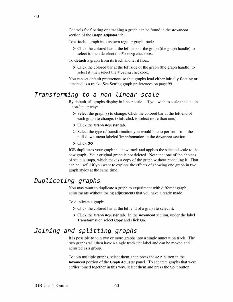
60
Controls for floating or attaching a graph can be found in the Advanced section of the Graph Adjuster tab.
To attach a graph into its own regular graph track:
➢ Click the colored bar at the left side of the graph (the graph handle) to select it, then deselect the Floating checkbox.
To detach a graph from its track and let it float:
➢ Click the colored bar at the left side of the graph (the graph handle) to select it, then select the Floating checkbox.
You can set default preferences so that graphs load either initially floating or attached as a track. See Setting graph preferences on page 99.
Transforming to a non-linear scaleBy default, all graphs display in linear scale. If you wish to scale the data in a nonlinear way:
➢ Select the graph(s) to change: Click the colored bar at the left end of each graph to change. (Shiftclick to select more than one.).
➢ Click the Graph Adjuster tab.
➢ Select the type of transformation you would like to perform from the pulldown menu labeled Transformation in the Advanced section.
➢ Click GO
IGB duplicates your graph in a new track and applies the selected scale to the new graph. Your original graph is not deleted. Note that one of the choices of scale is Copy, which makes a copy of the graph without rescaling it. That can be useful if you want to explore the effects of showing one graph in two graph styles at the same time.
Duplicating graphsYou may want to duplicate a graph to experiment with different graph adjustments without losing adjustments that you have already made.
To duplicate a graph:
➢ Click the colored bar at the left end of a graph to select it.
➢ Click the Graph Adjuster tab. In the Advanced section, under the label Transformation select Copy and click Go.
Joining and splitting graphsIt is possible to join two or more graphs into a single annotation track. The two graphs will then have a single track tier label and can be moved and adjusted as a group.
To join multiple graphs, select them, then press the Join button in the Advanced portion of the Graph Adjuster panel. To separate graphs that were earlier joined together in this way, select them and press the Split button.
IGB User’s Guide 60
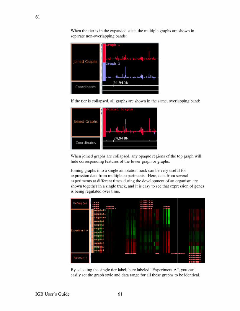
61
When the tier is in the expanded state, the multiple graphs are shown in separate nonoverlapping bands:
If the tier is collapsed, all graphs are shown in the same, overlapping band:
When joined graphs are collapsed, any opaque regions of the top graph will hide corresponding features of the lower graph or graphs.
Joining graphs into a single annotation track can be very useful for expression data from multiple experiments. Here, data from several experiments at different times during the development of an organism are shown together in a single track, and it is easy to see that expression of genes is being regulated over time.
By selecting the single tier label, here labeled “Experiment A”, you can easily set the graph style and data range for all these graphs to be identical.
IGB User’s Guide 61
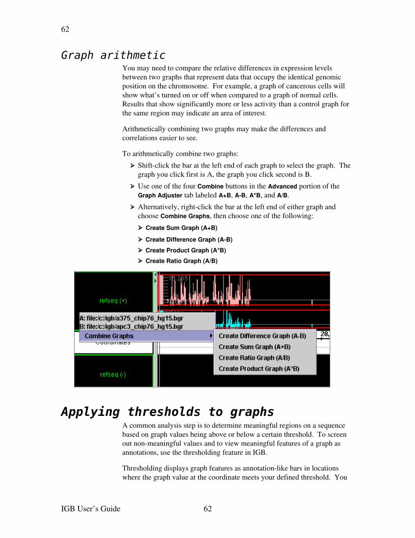
62
Graph arithmeticYou may need to compare the relative differences in expression levels between two graphs that represent data that occupy the identical genomic position on the chromosome. For example, a graph of cancerous cells will show what’s turned on or off when compared to a graph of normal cells. Results that show significantly more or less activity than a control graph for the same region may indicate an area of interest.
Arithmetically combining two graphs may make the differences and correlations easier to see.
To arithmetically combine two graphs:
➢ Shiftclick the bar at the left end of each graph to select the graph. The graph you click first is A, the graph you click second is B.
➢ Use one of the four Combine buttons in the Advanced portion of the Graph Adjuster tab labeled A+B, AB, A*B, and A/B.
➢ Alternatively, rightclick the bar at the left end of either graph and choose Combine Graphs, then choose one of the following:
➢ Create Sum Graph (A+B)
➢ Create Difference Graph (AB) ➢ Create Product Graph (A*B)
➢ Create Ratio Graph (A/B)
Applying thresholds to graphsA common analysis step is to determine meaningful regions on a sequence based on graph values being above or below a certain threshold. To screen out nonmeaningful values and to view meaningful features of a graph as annotations, use the thresholding feature in IGB.
Thresholding displays graph features as annotationlike bars in locations where the graph value at the coordinate meets your defined threshold. You
IGB User’s Guide 62
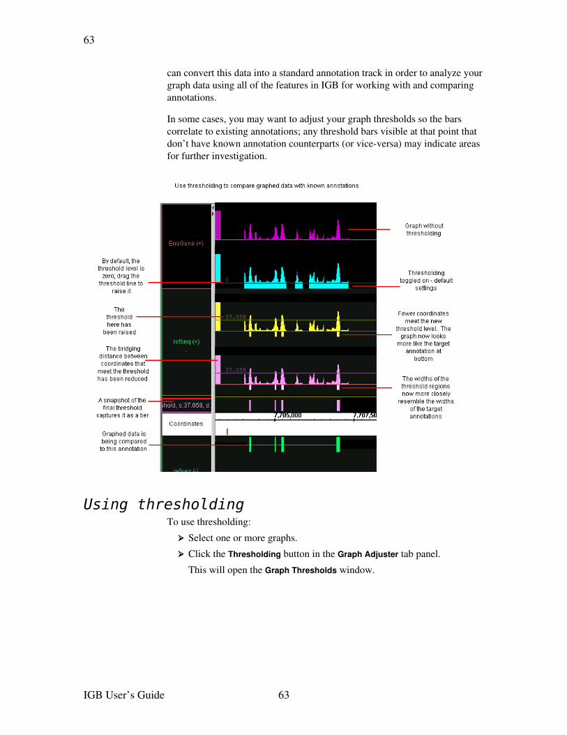
63
can convert this data into a standard annotation track in order to analyze your graph data using all of the features in IGB for working with and comparing annotations.
In some cases, you may want to adjust your graph thresholds so the bars correlate to existing annotations; any threshold bars visible at that point that don’t have known annotation counterparts (or viceversa) may indicate areas for further investigation.
Using thresholding To use thresholding:
➢ Select one or more graphs.
➢ Click the Thresholding button in the Graph Adjuster tab panel.
This will open the Graph Thresholds window.
IGB User’s Guide 63
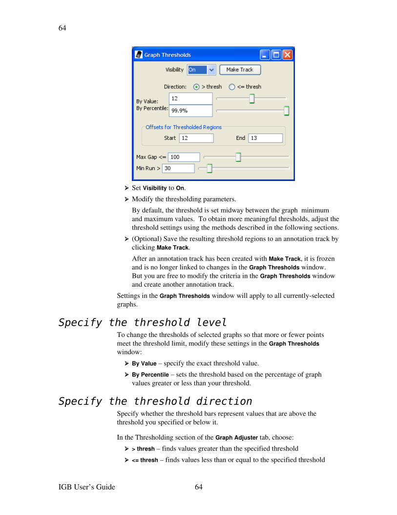
64
➢ Set Visibility to On.
➢ Modify the thresholding parameters.
By default, the threshold is set midway between the graph minimum and maximum values. To obtain more meaningful thresholds, adjust the threshold settings using the methods described in the following sections.
➢ (Optional) Save the resulting threshold regions to an annotation track by clicking Make Track.
After an annotation track has been created with Make Track, it is frozen and is no longer linked to changes in the Graph Thresholds window. But you are free to modify the criteria in the Graph Thresholds window and create another annotation track.
Settings in the Graph Thresholds window will apply to all currentlyselected graphs.
Specify the threshold levelTo change the thresholds of selected graphs so that more or fewer points meet the threshold limit, modify these settings in the Graph Thresholds window:
➢ By Value – specify the exact threshold value.
➢ By Percentile – sets the threshold based on the percentage of graph values greater or less than your threshold.
Specify the threshold directionSpecify whether the threshold bars represent values that are above the threshold you specified or below it.
In the Thresholding section of the Graph Adjuster tab, choose:
➢ > thresh – finds values greater than the specified threshold
➢ <= thresh – finds values less than or equal to the specified threshold
IGB User’s Guide 64
65
For example, for expression results graph score represents the level of hybridization activity. For a hybridization activity level to be considered significant, the score must be above a certain threshold. So you would choose the > thresh option and set your desired threshold value. If you need help to pick a threshold level, toggle the Yaxis on to see the graph’s scale on the Yaxis. See Graph labeling on page 59.
Control gapsExperimental data can be noisy. If you are looking for general trends and want to ignore small local variations, you can use the Max Gap and Min run settings.
Slide the sliders to adjust thresholding, or enter values into the boxes for each parameter:
➢ Max Gap: Groups of coordinates that meet the threshold may be separated by gaps where the threshold is not met. By default, thresholding bridges such gaps if they are less than 100 bps long. For example, if there are 300 bps that meet the threshold, then 99 bps that don’t, followed by 100 that do, the threshold bar would bridge the 99 bps to produce a single threshold annotation 499 bps long. To change the length of this bridge, enter a different value into the Max Gap textentry field.
➢ Min run: minimum number of bases in a row that must meet the threshold before an annotation bar will appear. For example, by default the Min run is 30 base pairs, so a sequence of 29 base pairs that meet the threshold will not be marked by an annotation bar.
Specify offsetsThe Offsets for Thresholded Regions feature is designed specifically for working with tiling array data.
Captured data from tiling array probes should usually be shifted for display. Since the probes are 25 base pairs long, but the xcoordinates given represent the starting coordinate, you should shift the threshold data so that it starts at 12 base pairs past the given beginning, and ends at 13 base pairs past the beginning. This is the default placement of all graph threshold bars.
If these offsets are not correct for the data you are analyzing, you should change them.
If you are viewing typical tiling array data, modify these settings in the Graph Thresholds window:
➢ Set the Start value to 12.
➢ Press the <Enter> key.
➢ Change the End value to 13, then press <Enter>.
IGB User’s Guide 65
66
When you view nontiling array data in IGB, you should adjust the offset to 0 to correctly align the threshold bars with their actual coordinates.
To adjust the offset values for nontiling array data modify these settings in the Graph Thresholds window:
➢ Set the Start value to 0.
➢ Press the <Enter> key.
➢ Change the End value to 1, then press <Enter>.
Capture the threshold barsCapture the threshold bars (which look similar to annotations) in their own track to more easily compare different threshold settings for a single graphed region. (See the thresholding illustration, above)
To capture the threshold bars and convert them to annotation tracks:
➢ Click to select the graph
➢ Click the Make Track button.
A snapshot of the current thresholded graph will be created as a new annotation track. This track will be given a default label which you can later change if desired.
To permanently capture the threshold snapshot for later use or sharing:
➢ Rightclick the track and choose Save Annotations.
➢ Choose one of the file formats.
➢ Name your file. Be sure to include the correct filename extension.
After you have captured threshold “annotations” from a graph or other set of data, you can examine these “annotations” using all of the tools in IGB for working with and comparing annotations.
Useful graph customizationsSome common useful graph customizations are:
➢ Dampen the distorting effects of outliers – for example, ignore any points that are above the 99.5th percentile or below the .05th percentile. This makes it easier to see the bulk of your data.
Under YAxis Scale, set By Percentile to the desired lower and upper percentile bounds.
➢ Apply matching scales when comparing multiple graphs. For example, if one graph has a minimum value of 12 and a max value of 24, and another has a min value of 24 and a max value of 48, make them easier to compare by changing the visible bounds so they have the same scale. For each graph being compared, toggle the Yaxis on to view the min and max values for each, then adjust the YAxis Scale using By Value to make them compatible
IGB User’s Guide 66
67
➢ Display the optimal type of graph for a particular purpose, for example use a stairstep style graph for analyzing ESTs or performing other density analyses. Then slice the selection to see details.
➢ Use the thresholding feature to find areas of activity that may be significant, for example areas that do not coincide with known exons. Adjust your threshold bars to match the known annotations; any “extra” threshold bars visible in your graph indicate potential areas of interest.
Getting details about a graphTextual information about some graphs is available in Selection Info.
Click the colored bar at the left of the graph, then click the Selection Info tab. Resize the columns if needed.
Saving and bookmarking graphsMost graph properties that you set in IGB can be captured for future use by saving or bookmarking.
Saving graph data as a fileYou can save a graph as a separate file for future reference or off line use. Note that this saves only the graph data, without any visualization customizations you may have made to it.
To save graph data to a file:
➢ Select the graph by clicking the colored bar at the left end of the graph.
➢ Click the Graph Adjuster tab. Click the Save button.
➢ Specify location and graph name.
➢ Pick one of the graph formats offered. Typically choose “.egr” format for interval graphs and “.sgr” format for other graphs.
➢ You will be prompted to add the proper “.sgr” or “.egr” filename extension depending on the type of graph data.
➢ Click OK.
Graph properties, such as color, scale, and so forth, may not be saved along with the data. Some graph formats, such as “.bed”, “.gff”, and “.wig” allow such properties to be specified in “track lines”.
Bookmarking graph viewsBy creating a bookmark, you can save a link to your graph along with the customizations you have made to its appearance. See Bookmarking on page 76.
You can also export your list of bookmarks to share it with other users. If your bookmarks contain links to graph files on your file system, those files may not be available to users on other file systems.
IGB User’s Guide 67
68
Printing graphsTo print directly to your printer:
➢ Choose File menu > Print.
You can also print to an EPS format file. Files in the EPS format print in highresolution and can be imported into many graphics programs. Files printed in EPS format are suitable for use in publications. To print to an EPS file:
➢ Choose File menu > Export.
➢ Choose to export either the Main View or Main View (With Labels)
➢ Choose a name for your file, using the extension “.eps” .
Setting graph preferencesTo set preferences that apply by default when you load graphs, see Settinggraph preferences on page 99.
IGB User’s Guide 68
69
Visualizing probe sets
IntroductionIGB can be used to visualize data from Affymetrix showing the locations of GeneChip Expression Array probe sets aligned to a genome.
Chip design procedures have varied somewhat from chip to chip, but, in general, probes on Affymetrix’s standard commercial expression microarrays (such as the Human U133 chip) are designed to match the 3’ regions of known or computed mRNA sequences. These probes are typically 18 to 25 bases long depending on the chip.
In standard arrays, probes are grouped conceptually into probe sets, groups of probes that are expected to measure expression for individual known or computationallydeduced mRNA molecules.
Probe sequences are typically selected from the 3’ regions of these design sequences in order to maximize the amount of sample mRNA to be measured. (This socalled “3prime bias” will most likely change as sample preparation protocols improve over time.)
These design sequences may be identical to known mRNA sequences in GenBank, or they may have been produced computationally by merging ESTs or mRNA sequences into a single sequence, sometimes called a “consensus” sequence.
IGB can be used to visualize the location of design sequences and probes within the genomic sequence. Seeing where these sequences are located within the genome can be extremely useful when several overlapping probe sets recognize diverse mRNAs originating from the same gene. Around 60% of human genes produce multiple variants, and these diverse variants often exhibit very complex configurations of exons and introns. As a result, it often helps to be able to view a diagram of these complex structures together with probes in order to determine which individual mRNAs are being detected by a given probe set.
To make this easier, IGB shows where the design sequences and their probes align to the genome together with alignments between the genomic sequence and known or predicted mRNAs. By showing probes, known mRNAs, and design sequences in the same view, IGB makes it possible to determine quickly which known mRNA a probe set could detect.
However, it is important to note that these genome alignments can only be as good as the genomic sequence on which they are based. Genomes vary in their level of quality – for example, the human and fruit fly genomes are very high quality, having gone through several releases involving many
IGB User’s Guide 69
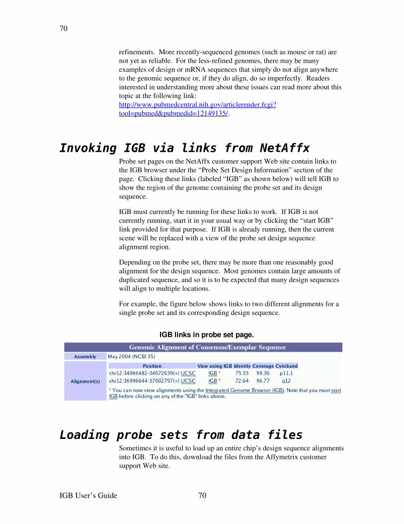
70
refinements. More recentlysequenced genomes (such as mouse or rat) are not yet as reliable. For the lessrefined genomes, there may be many examples of design or mRNA sequences that simply do not align anywhere to the genomic sequence or, if they do align, do so imperfectly. Readers interested in understanding more about these issues can read more about this topic at the following link: http://www.pubmedcentral.nih.gov/articlerender.fcgi?tool=pubmed&pubmedid=12149135/.
Invoking IGB via links from NetAffxProbe set pages on the NetAffx customer support Web site contain links to the IGB browser under the “Probe Set Design Information” section of the page. Clicking these links (labeled “IGB” as shown below) will tell IGB to show the region of the genome containing the probe set and its design sequence.
IGB must currently be running for these links to work. If IGB is not currently running, start it in your usual way or by clicking the “start IGB” link provided for that purpose. If IGB is already running, then the current scene will be replaced with a view of the probe set design sequence alignment region.
Depending on the probe set, there may be more than one reasonably good alignment for the design sequence. Most genomes contain large amounts of duplicated sequence, and so it is to be expected that many design sequences will align to multiple locations.
For example, the figure below shows links to two different alignments for a single probe set and its corresponding design sequence.
Loading probe sets from data filesSometimes it is useful to load up an entire chip’s design sequence alignments into IGB. To do this, download the files from the Affymetrix customer support Web site.
IGB User’s Guide 70
IGB links in probe set page.
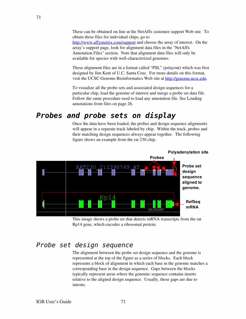
71
These can be obtained online at the NetAffx customer support Web site. To obtain these files for individual chips, go to http://www.affymetrix.com/support and choose the array of interest. On the array’s support page, look for alignment data files in the "NetAffx Annotation Files" section. Note that alignment data files will only be available for species with wellcharacterized genomes.
These alignment files are in a format called “PSL” (pslayout) which was first designed by Jim Kent of U.C. Santa Cruz. For more details on this format, visit the UCSC Genome Bioinformatics Web site at http://genome.ucsc.edu.
To visualize all the probe sets and associated design sequences for a particular chip, load the genome of interest and merge a probe set data file. Follow the same procedure used to load any annotation file. See Loadingannotations from files on page 26.
Probes and probe sets on displayOnce the data have been loaded, the probes and design sequence alignments will appear in a separate track labeled by chip. Within the track, probes and their matching design sequences always appear together. The following figure shows an example from the rat 230 chip.
This image shows a probe set that detects mRNA transcripts from the rat Rp14 gene, which encodes a ribosomal protein.
Probe set design sequenceThe alignment between the probe set design sequence and the genome is represented at the top of the figure as a series of blocks. Each block represents a block of alignment in which each base in the genome matches a corresponding base in the design sequence. Gaps between the blocks typically represent areas where the genomic sequence contains inserts relative to the aligned design sequence. Usually, these gaps are due to introns.
IGB User’s Guide 71
Probe set design sequence aligned to genome.
RefSeqmRNA
ProbesPolyadenylation site
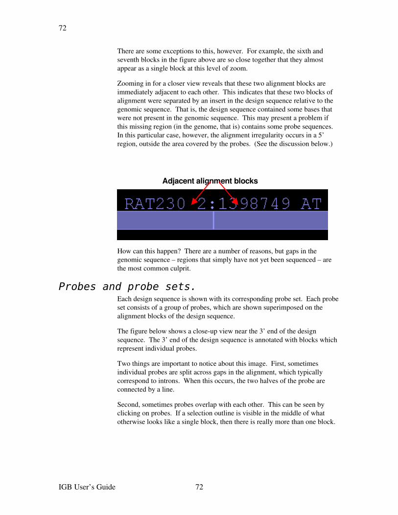
72
There are some exceptions to this, however. For example, the sixth and seventh blocks in the figure above are so close together that they almost appear as a single block at this level of zoom.
Zooming in for a closer view reveals that these two alignment blocks are immediately adjacent to each other. This indicates that these two blocks of alignment were separated by an insert in the design sequence relative to the genomic sequence. That is, the design sequence contained some bases that were not present in the genomic sequence. This may present a problem if this missing region (in the genome, that is) contains some probe sequences. In this particular case, however, the alignment irregularity occurs in a 5’ region, outside the area covered by the probes. (See the discussion below.)
How can this happen? There are a number of reasons, but gaps in the genomic sequence – regions that simply have not yet been sequenced – are the most common culprit.
Probes and probe sets.Each design sequence is shown with its corresponding probe set. Each probe set consists of a group of probes, which are shown superimposed on the alignment blocks of the design sequence.
The figure below shows a closeup view near the 3’ end of the design sequence. The 3’ end of the design sequence is annotated with blocks which represent individual probes.
Two things are important to notice about this image. First, sometimes individual probes are split across gaps in the alignment, which typically correspond to introns. When this occurs, the two halves of the probe are connected by a line.
Second, sometimes probes overlap with each other. This can be seen by clicking on probes. If a selection outline is visible in the middle of what otherwise looks like a single block, then there is really more than one block.
IGB User’s Guide 72
Adjacent alignment blocks
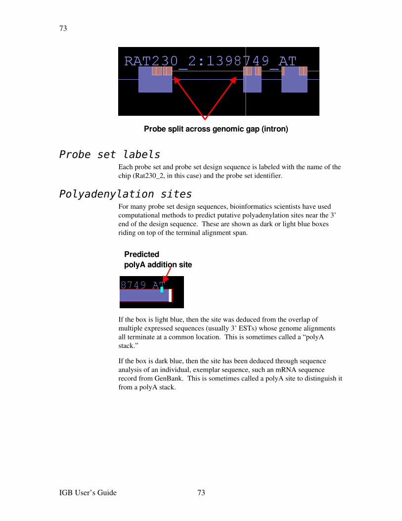
73
Probe set labelsEach probe set and probe set design sequence is labeled with the name of the chip (Rat230_2, in this case) and the probe set identifier.
Polyadenylation sites For many probe set design sequences, bioinformatics scientists have used computational methods to predict putative polyadenylation sites near the 3’ end of the design sequence. These are shown as dark or light blue boxes riding on top of the terminal alignment span.
If the box is light blue, then the site was deduced from the overlap of multiple expressed sequences (usually 3’ ESTs) whose genome alignments all terminate at a common location. This is sometimes called a “polyA stack.”
If the box is dark blue, then the site has been deduced through sequence analysis of an individual, exemplar sequence, such an mRNA sequence record from GenBank. This is sometimes called a polyA site to distinguish it from a polyA stack.
IGB User’s Guide 73
Probe split across genomic gap (intron)
Predicted polyA addition site
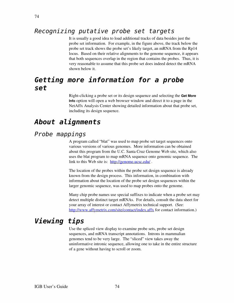
74
Recognizing putative probe set targetsIt is usually a good idea to load additional tracks of data besides just the probe set information. For example, in the figure above, the track below the probe set track shows the probe set’s likely target, an mRNA from the Rp14 locus. Based on their relative alignments to the genome sequence, it appears that both sequences overlap in the region that contains the probes. Thus, it is very reasonable to assume that this probe set does indeed detect the mRNA shown below it.
Getting more information for a probe set
Rightclicking a probe set or its design sequence and selecting the Get More Info option will open a web browser window and direct it to a page in the NetAffx Analysis Center showing detailed information about that probe set, including its design sequence.
About alignments
Probe mappingsA program called “blat” was used to map probe set target sequences onto various versions of various genomes. More information can be obtained about this program from the U.C. Santa Cruz Genome Web site, which also uses the blat program to map mRNA sequence onto genomic sequence. The link to this Web site is: http://genome.ucsc.edu/ .
The location of the probes within the probe set design sequence is already known from the design process. This information, in combination with information about the location of the probe set design sequences within the larger genomic sequence, was used to map probes onto the genome.
Many chip probe names use special suffixes to indicate when a probe set may detect multiple distinct target mRNAs. For details, consult the data sheet for your array of interest or contact Affymetrix technical support. (See: http://www.affymetrix.com/site/contact/index.affx for contact information.)
Viewing tipsUse the spliced view display to examine probe sets, probe set design sequences, and mRNA transcript annotations. Introns in mammalian genomes tend to be very large. The “sliced” view takes away the uninformative intronic sequence, allowing one to take in the entire structure of a gene without having to scroll or zoom.
IGB User’s Guide 74
75
Capturing, saving, and sharing data
There are several ways to save data for use in other applications, sharing, or later use in IGB.
Save or share data from IGB in any of several ways
➢ Viewing a region in the UCSC browser
➢ Saving annotation tracks
➢ Copying sequence bases
➢ Saving graph files
➢ Bookmarking
➢ Copying data from table cells
➢ Printing
Viewing a region in the UCSC browser The UCSC web genome browser is a rich source of genomic information.
For more information on what’s available there, visit http://genome.ucsc.edu/.
To view in the UCSC browser the same region currently displayed in IGB:
➢ Select an item in the viewer window
➢ Choose View menu > View region in UCSC browser
Results may be slow to appear. (You may want to set your web browser preferences to show loading progress for example, Microsoft Internet Explorer has a bar on the bottom of the web window. See the documentation for your web browser.)
Saving annotation tracksIGB is mainly designed for viewing existing data, not producing new data files. Nonetheless, you can save any single annotation track to a file by selecting the track tier label, performing a rightclick and selecting Save to file. You will be given the option of saving in several formats, such as BED and DAS/2 XML.
Copying sequence basesYou can copy a sequence of bases to the clipboard and paste the sequence into another application for use there.
IGB User’s Guide 75
76
See Copying sequence bases on page 33.
Saving graph filesSee Saving graph data as a file on page 67.
BookmarkingTo return later to a region or annotation and zoom level of interest, you can bookmark it. Items that you bookmark will appear under the Bookmarks menu. You can edit your bookmark list, as well as exporting and importing bookmark lists, with the Bookmark Manager window.
Any bookmarks that you create during a session will be saved when you exit, and will be available the next time you launch IGB.
Creating bookmarksBefore you add bookmarks, make sure you are not running multiple instances of IGB.
There are two types of bookmarks in IGB:
➢ Position bookmarks. These record the currently shown genome, the location, and the current zoom level.
➢ To create, choose Bookmarks menu > Add position bookmark
➢ Positionandgraphs bookmarks. These record the same things as position bookmarks, but also keep track of any graphs that you have loaded thus far. In addition to remembering the data files that you have loaded, positionandgraphs bookmarks can also remember many of your customizations for graph appearance, such as color, graph bound adjustments, thresholding, and labeling.
➢ To create, choose Bookmarks menu > Add position & graphs bookmark.
Using bookmarksTo load a view that you have bookmarked.
➢ Choose Bookmarks menu > [name of your bookmark].
Viewing and changing bookmark detailsYou can view details about your bookmarks, such as their position, which genome they refer to, or customizations for positionandgraphs bookmarks. You can also modify some details, such as the name of a bookmark or customizations of a positionandgraphs bookmark.
To view or change bookmark details:
➢ Click Bookmarks menu > Manage Bookmarks.
➢ Select a bookmark.
IGB User’s Guide 76
77
➢ Right click the selected bookmark or click the Bookmarks menu in the Bookmark Manager window and then select the Properties button.
➢ The information will appear in tabular format in a new window.
➢ (Optional) Modify the bookmark details.
➢ Click Apply Changes or Cancel. Changes will not take effect unless you chose Apply Changes.
Exporting bookmarksTo save a copy of the bookmarks to a file:
➢ Click Bookmarks menu > Manage Bookmarks.
➢ In the bookmark manager window, choose Bookmarks menu > Export Bookmarks
Bookmarks are saved in a single file in the Netscape bookmarks file format. This format resembles XML and HTML, but is not identical to either of those, so use caution if you choose to edit the file.
Importing bookmarksYou can import and use bookmarks, for example bookmarks that other people give you:
➢ Click Bookmarks menu > Manage Bookmarks.
➢ In the bookmark manager window, choose Bookmarks menu > Import Bookmarks > choose the file containing the bookmark of interest.
You can import multiple sets of bookmarks during the same IGB session. Imported bookmarks will be added to the end of the list of existing bookmarks. All imported bookmarks will be persistent between sessions of IGB.
Copying data from table cellsYou can copy and paste table cells from the Selection Info panel (or most other tables) to the clipboard and paste them into Excel or some other program.
To capture data in table cells:
➢ Click and drag to select the cells you want.
➢ Copy (using ControlC) and then paste into the target application.
PrintingTo print directly to your printer:
➢ Choose File menu > Print.
You can also print to an EPS format file. Files in the EPS format print in highresolution and can be imported into many graphics programs. Files
IGB User’s Guide 77

78
printed in EPS format are suitable for use in publications. To print to an EPS file:
➢ Choose File menu > Export.
➢ Choose to export either the Main View or Main View (With Labels) or Sliced View (With Labels).
➢ Choose a name for your file, using the extension “.eps”.
IGB User’s Guide 78
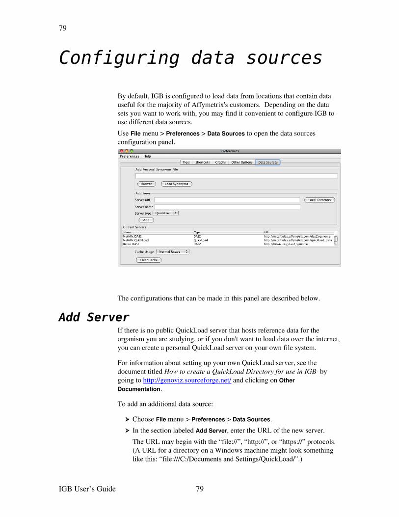
79
Configuring data sources
By default, IGB is configured to load data from locations that contain data useful for the majority of Affymetrix's customers. Depending on the data sets you want to work with, you may find it convenient to configure IGB to use different data sources.
Use File menu > Preferences > Data Sources to open the data sources configuration panel.
The configurations that can be made in this panel are described below.
Add ServerIf there is no public QuickLoad server that hosts reference data for the organism you are studying, or if you don't want to load data over the internet, you can create a personal QuickLoad server on your own file system.
For information about setting up your own QuickLoad server, see the document titled How to create a QuickLoad Directory for use in IGB by going to http://genoviz.sourceforge.net/ and clicking on Other Documentation.
To add an additional data source:
➢ Choose File menu > Preferences > Data Sources.
➢ In the section labeled Add Server, enter the URL of the new server.
The URL may begin with the “file://”, “http://”, or “https://” protocols. (A URL for a directory on a Windows machine might look something like this: “file:///C:/Documents and Settings/QuickLoad/”.)
IGB User’s Guide 79
80
If this is a local QuickLoad server, you can use the Local Directory button to easily browse to this directory.)
➢ Choose a unique name for this new server.
➢ Choose the server type (DAS/1, DAS/2, or QuickLoad).
➢ Click Add.
Your new server will be available to use immediately. The default servers will still be available to you. You can freely switch between servers while IGB is running by using the controls in the Data Access tab panel.
If your server does not appear to be working, check the messages in the IGB console. You may have typed the URL incorrectly, or you may have forgotten to include some of the necessary configuration files.
Note that the QuickLoad system is designed for loading common reference data files. It is best to store your experimental data elsewhere.
SynonymsDifferent data sources often refer to the same genome version or chromosome by different names. What NCBI refers to as human genome build 35 is known as hg17 at UCSC and can also be called ensembl1834 or H_sapiens_May_2004. Human chromosome 2 is identified sometimes as “chr2”, or “chrom 2” or simply “2”.
When IGB is able to recognize that two names refer to the same genome or chromosome, it will merge the data. Otherwise it will keep the two data sets distinct.
IGB uses a simple table of synonyms to store these associations. The default QuickLoad server used by IGB stores a default synonyms file. (This default file is at http://netaffxdas.affymetrix.com/quickload_data/synonyms.txt)
You can create your own set of synonyms that will extend this set if needed. If you have created your own QuickLoad server you can place your synonyms file on that server. You can also load an additional personal synonyms file from your computer file system.
To add a personal synonyms file:
➢ Choose File menu > Preferences > Data Sources.
➢ Use the Browse button to locate the file.
➢ Press Load Synonyms.
The format is a simple tabdelimited file where each row contains a list of synonyms separated by tabs. Every term in each row is considered synonymous. In addition, the synonyms are transitive, such that if “A” is a synonym of “B” and “B” is a synonym of “C”, then “A” is automatically considered a synonym of “C”.
IGB User’s Guide 80
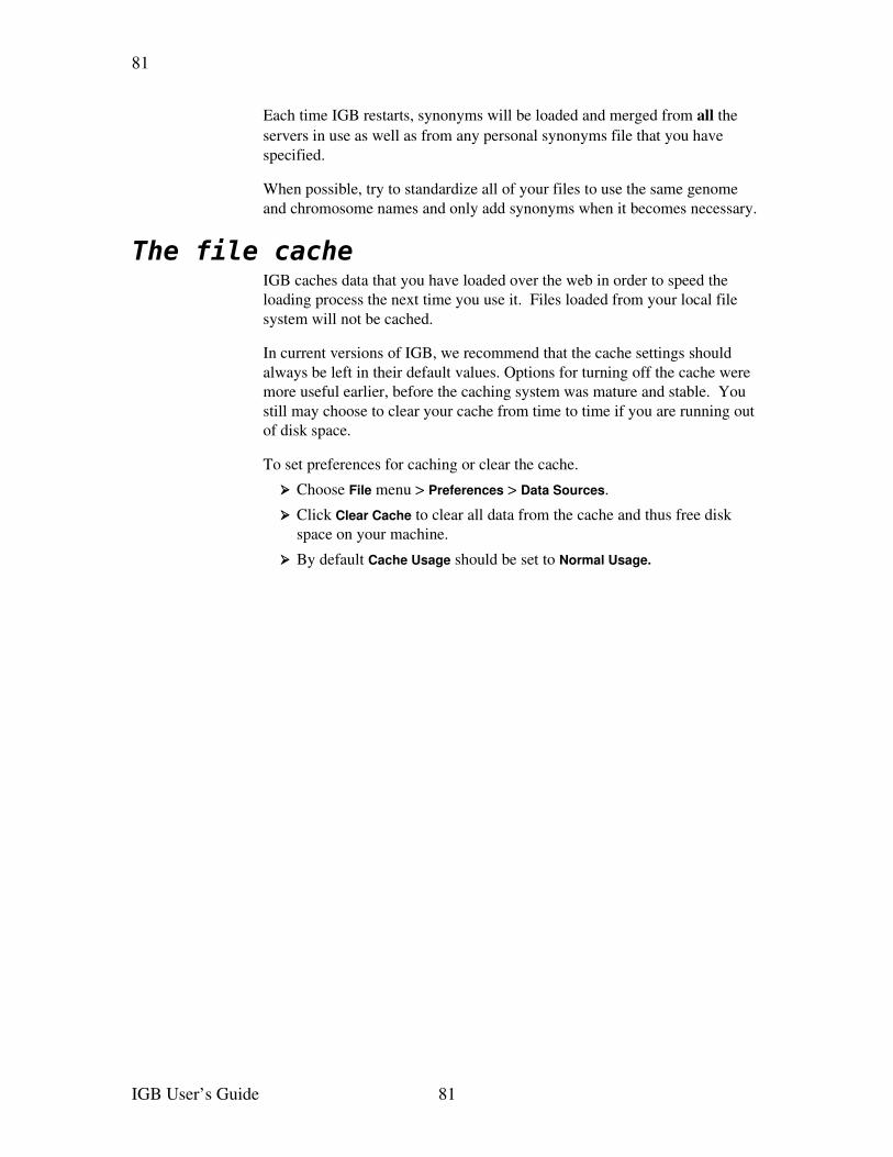
81
Each time IGB restarts, synonyms will be loaded and merged from all the servers in use as well as from any personal synonyms file that you have specified.
When possible, try to standardize all of your files to use the same genome and chromosome names and only add synonyms when it becomes necessary.
The file cacheIGB caches data that you have loaded over the web in order to speed the loading process the next time you use it. Files loaded from your local file system will not be cached.
In current versions of IGB, we recommend that the cache settings should always be left in their default values. Options for turning off the cache were more useful earlier, before the caching system was mature and stable. You still may choose to clear your cache from time to time if you are running out of disk space.
To set preferences for caching or clear the cache.
➢ Choose File menu > Preferences > Data Sources.
➢ Click Clear Cache to clear all data from the cache and thus free disk space on your machine.
➢ By default Cache Usage should be set to Normal Usage.
IGB User’s Guide 81
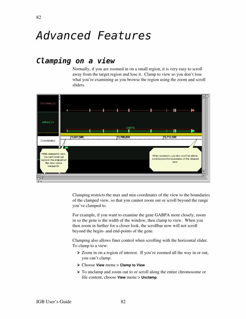
82
Advanced Features
Clamping on a viewNormally, if you are zoomed in on a small region, it is very easy to scroll away from the target region and lose it. Clamp to view so you don’t lose what you’re examining as you browse the region using the zoom and scroll sliders.
Clamping restricts the max and min coordinates of the view to the boundaries of the clamped view, so that you cannot zoom out or scroll beyond the range you’ve clamped to.
For example, if you want to examine the gene GABPA more closely, zoom in so the gene is the width of the window, then clamp to view. When you then zoom in further for a closer look, the scrollbar now will not scroll beyond the begin and endpoints of the gene.
Clamping also allows finer control when scrolling with the horizontal slider. To clamp to a view:
➢ Zoom in on a region of interest. If you’re zoomed all the way in or out, you can’t clamp.
➢ Choose View menu > Clamp to View
➢ To unclamp and zoom out to or scroll along the entire chromosome or file content, choose View menu > Unclamp.
IGB User’s Guide 82
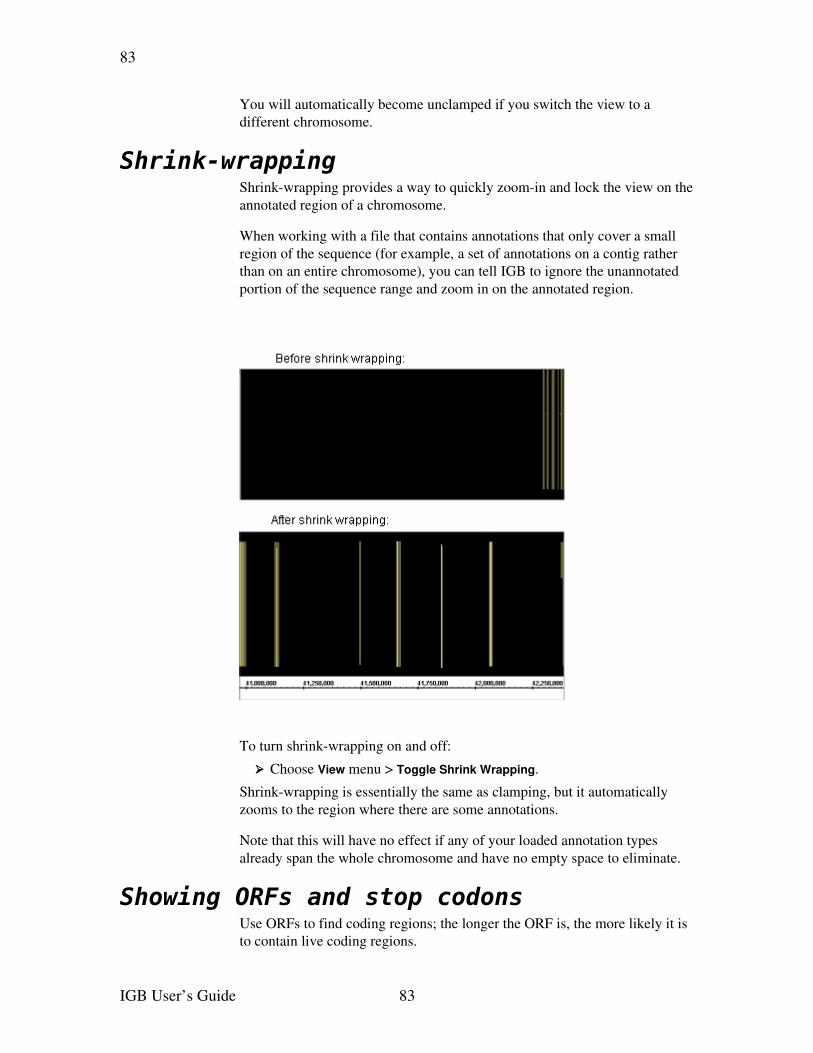
83
You will automatically become unclamped if you switch the view to a different chromosome.
Shrink-wrappingShrinkwrapping provides a way to quickly zoomin and lock the view on the annotated region of a chromosome.
When working with a file that contains annotations that only cover a small region of the sequence (for example, a set of annotations on a contig rather than on an entire chromosome), you can tell IGB to ignore the unannotated portion of the sequence range and zoom in on the annotated region.
To turn shrinkwrapping on and off:
➢ Choose View menu > Toggle Shrink Wrapping.
Shrinkwrapping is essentially the same as clamping, but it automatically zooms to the region where there are some annotations.
Note that this will have no effect if any of your loaded annotation types already span the whole chromosome and have no empty space to eliminate.
Showing ORFs and stop codons Use ORFs to find coding regions; the longer the ORF is, the more likely it is to contain live coding regions.
IGB User’s Guide 83
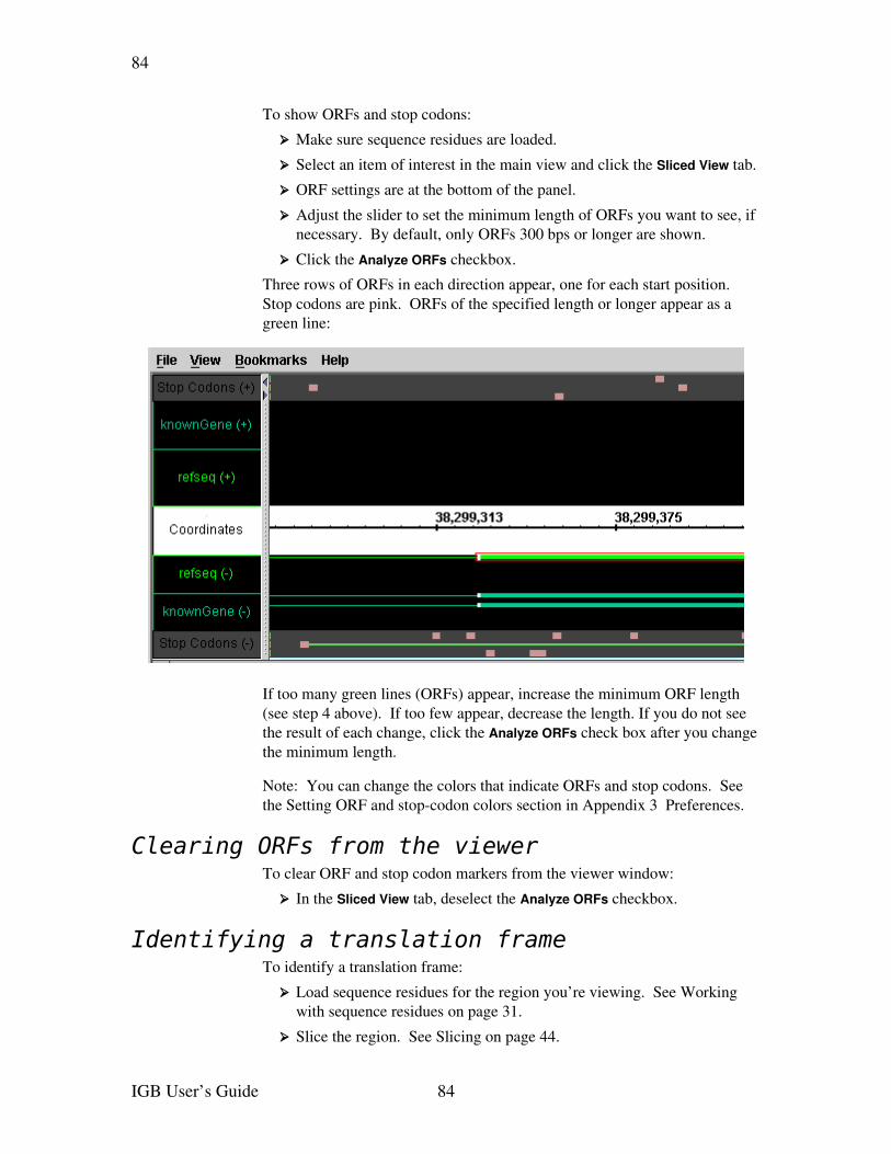
84
To show ORFs and stop codons:
➢ Make sure sequence residues are loaded.
➢ Select an item of interest in the main view and click the Sliced View tab.
➢ ORF settings are at the bottom of the panel.
➢ Adjust the slider to set the minimum length of ORFs you want to see, if necessary. By default, only ORFs 300 bps or longer are shown.
➢ Click the Analyze ORFs checkbox.
Three rows of ORFs in each direction appear, one for each start position. Stop codons are pink. ORFs of the specified length or longer appear as a green line:
If too many green lines (ORFs) appear, increase the minimum ORF length (see step 4 above). If too few appear, decrease the length. If you do not see the result of each change, click the Analyze ORFs check box after you change the minimum length.
Note: You can change the colors that indicate ORFs and stop codons. See the Setting ORF and stopcodon colors section in Appendix 3 Preferences.
Clearing ORFs from the viewerTo clear ORF and stop codon markers from the viewer window:
➢ In the Sliced View tab, deselect the Analyze ORFs checkbox.
Identifying a translation frameTo identify a translation frame:
➢ Load sequence residues for the region you’re viewing. See Workingwith sequence residues on page 31.
➢ Slice the region. See Slicing on page 44.
IGB User’s Guide 84
85
➢ Adjust the slicing to a buffer of 0 bases to completely remove the introns.
➢ Analyze the ORFs as above.
➢ Look for the long, continuous green line that corresponds to your strungtogether exon set. This is your translation frame.
➢ Currently, if a stop codon is located beyond the region being viewed, the green line is not visible; instead, the evidence of a translation frame is the lack of stop codons over a long sequence.
Interacting with other genome browsersIGB can be used in conjunction with other applications, including webbased genome browsers. Webbased browsers have the advantages of being installed and maintained on a remote computer, and of giving you access to large amounts of remotelystored data. IGB, and other standalone applications, have the advantages of more rapid navigation, ability to work when offline, and secure access to private, local data. It is thus natural that users will make use of webbased applications along with IGB.
Webbased browsers include
➢ The UCSC Genome Browser
http://genome.ucsc.edu/
➢ GBrowse, from the Generic Model Organism Database project
http://www.gmod.org/
By using some of the standardized data file formats, such as FASTA for sequences, data files can be used in multiple applications.
IGB contains a menu item that will open the UCSC browser on the same region you are currently viewing. IGB also allows the configuration of selectionbased links to other webpages.
The reverse process is also possible. Web pages and other programs can control IGB through the use of hyperlinks. See the section Controlling IGBthrough a browser below.
To facilitate sharing of data files between IGB and the UCSC browser, IGB allows the use of track lines to specify some display properties. Since these track lines were defined by UCSC for use in their browser, not all properties are directly applicable in IGB, but those which are applicable are used. See
http://genome.ucsc.edu/goldenPath/help/customTrack.html#TRACK
Track linesFor many textbased file formats, it is possible to configure the track name, color, and other properties through the use of track lines in the file header or comments. Track lines were invented for use in the UCSC genome browser,
IGB User’s Guide 85
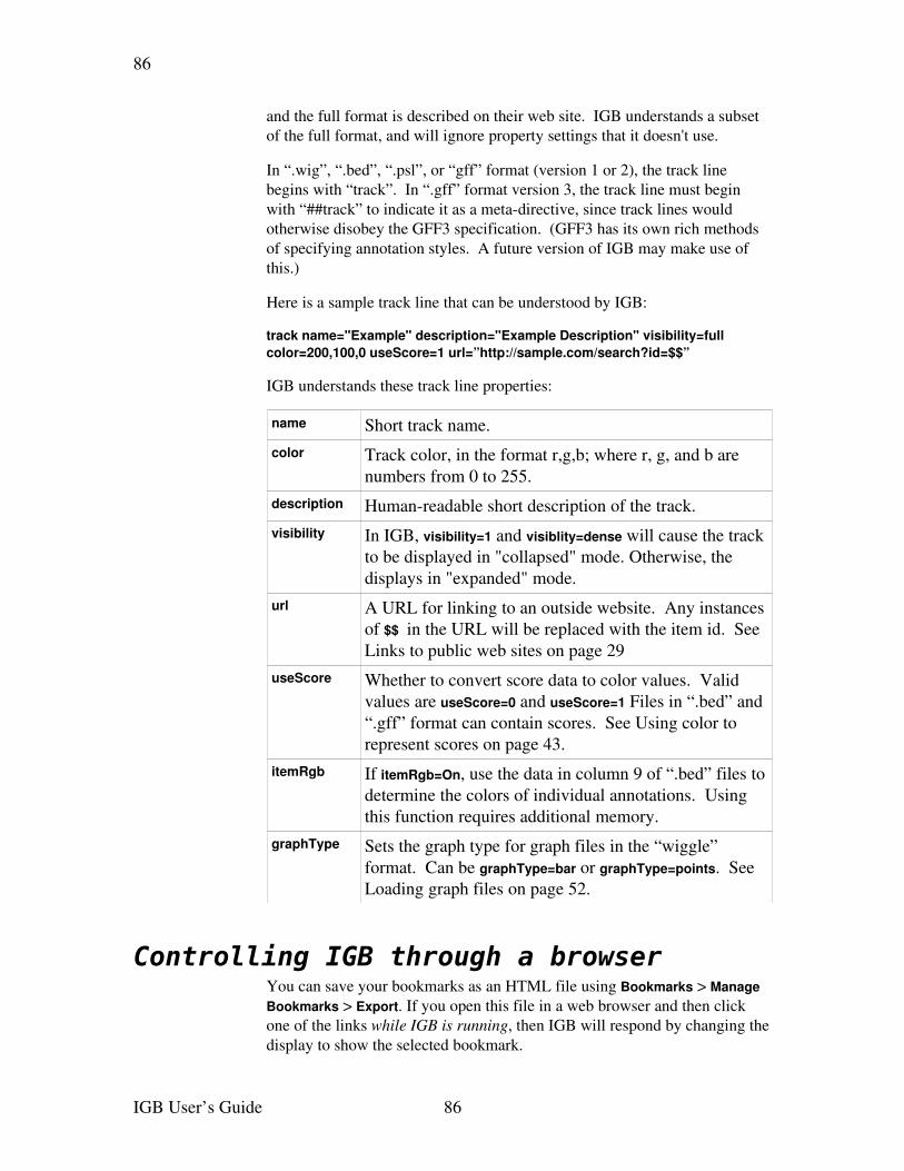
86
and the full format is described on their web site. IGB understands a subset of the full format, and will ignore property settings that it doesn't use.
In “.wig”, “.bed”, “.psl”, or “gff” format (version 1 or 2), the track line begins with “track”. In “.gff” format version 3, the track line must begin with “##track” to indicate it as a metadirective, since track lines would otherwise disobey the GFF3 specification. (GFF3 has its own rich methods of specifying annotation styles. A future version of IGB may make use of this.)
Here is a sample track line that can be understood by IGB:
track name="Example" description="Example Description" visibility=full color=200,100,0 useScore=1 url=”http://sample.com/search?id=$$”
IGB understands these track line properties:
name Short track name.color Track color, in the format r,g,b; where r, g, and b are
numbers from 0 to 255.description Humanreadable short description of the track.visibility In IGB, visibility=1 and visiblity=dense will cause the track
to be displayed in "collapsed" mode. Otherwise, the displays in "expanded" mode.
url A URL for linking to an outside website. Any instances of $$ in the URL will be replaced with the item id. See Links to public web sites on page 29
useScore Whether to convert score data to color values. Valid values are useScore=0 and useScore=1 Files in “.bed” and “.gff” format can contain scores. See Using color torepresent scores on page 43.
itemRgb If itemRgb=On, use the data in column 9 of “.bed” files to determine the colors of individual annotations. Using this function requires additional memory.
graphType Sets the graph type for graph files in the “wiggle” format. Can be graphType=bar or graphType=points. See Loading graph files on page 52.
Controlling IGB through a browserYou can save your bookmarks as an HTML file using Bookmarks > Manage Bookmarks > Export. If you open this file in a web browser and then click one of the links while IGB is running, then IGB will respond by changing the display to show the selected bookmark.
IGB User’s Guide 86
87
This will only work for the first instance of IGB that you are running. For example, if you are running two copies of IGB, then the browser will only affect the IGB window that you started first.
This same feature can be used by any web page or any program that is capable of sending an http request. The NetAffx Analysis Center on the Affymetrix website makes use of this feature.
The following is a simple description of how this works. The control commands include more options than shown here. Interested developers should contact the IGB development team.
If you open a bookmarks file in a text editor, you will find that the URL for each bookmark looks something like http://localhost:7085/UnibrowControl?seqid=chr21&version=Human_May_2004&start=44534188&end=44542686.
Here “localhost:7085” refers to port 7085 on your local machine. IGB, by default, “listens” to port 7085 on whatever machine it happens to be running. So if a Web browser sends a request to “localhost:7085,” IGB will hear it and respond. If the URL contains the right parameters (version, seqid, start, end, etc.) then IGB responds by showing the genomic “scene” described in the bookmark.
However, if you start up a new instance of IGB while one is already running, which we do not recommend, the new instance will listen to a different port – the first port above 7085 that happens to be vacant. This is why the bookmark links will only work for the first IGB instance and not for any others you start running after that.
IGB User’s Guide 87
88
Appendix 1 Java Web Start
We recommend a free utility from Sun Microsystems called Java Web Start to simplify installation and updating of IGB. When you launch IGB with this utility, it will download and install updates as they become available.
In many cases, the Java Runtime Environment, including Java Web Start, will already be installed on your machine by default. (In the past it was necessary to install Web Start separately, but now Java Web Start is a standard component of the Java Runtime Environment.) We strongly recommend you use a recent version of Web Start. Versions prior to 1.4.2 have problems that may sometimes interfere with launching IGB.
The following information is current at the time this document was written. What you will see on Sun’s web site is subject to change.
To use IGB with Java Web Start:
➢ Go to the Bioviz site for IGB: http://igb.bioviz.org/download.shtml . If you see buttons labeled “Launch IGB” or something similar, then Java Web Start is already installed on your computer and you can start IGB by pressing one of those buttons.
If you do not see those buttons, continue with the rest of these instructions.
➢ Go directly to http://java.com
➢ Click the link “Download Now”.
➢ Click to download the application for the platform that you are using (Windows, Linux, etc.) You can use either the offline or the regular version.
➢ Read and accept the license.
➢ Click Open to run the installation from the Sun server, or click Save to save the installer to your hard disk and run the installation from there. When you run the installer, you can accept the defaults.
➢ After installation is complete, close down and restart your browser.
➢ Return to the web page listed in the first step of this procedure and click the Launch IGB button.
➢ You may see a message asking if you would like to integrate IGB into your desktop environment.
If you wish to place a shortcut to IGB on your desktop and in your Start menu > Programs, click Yes. Otherwise, click No
IGB will launch.
IGB User’s Guide 88
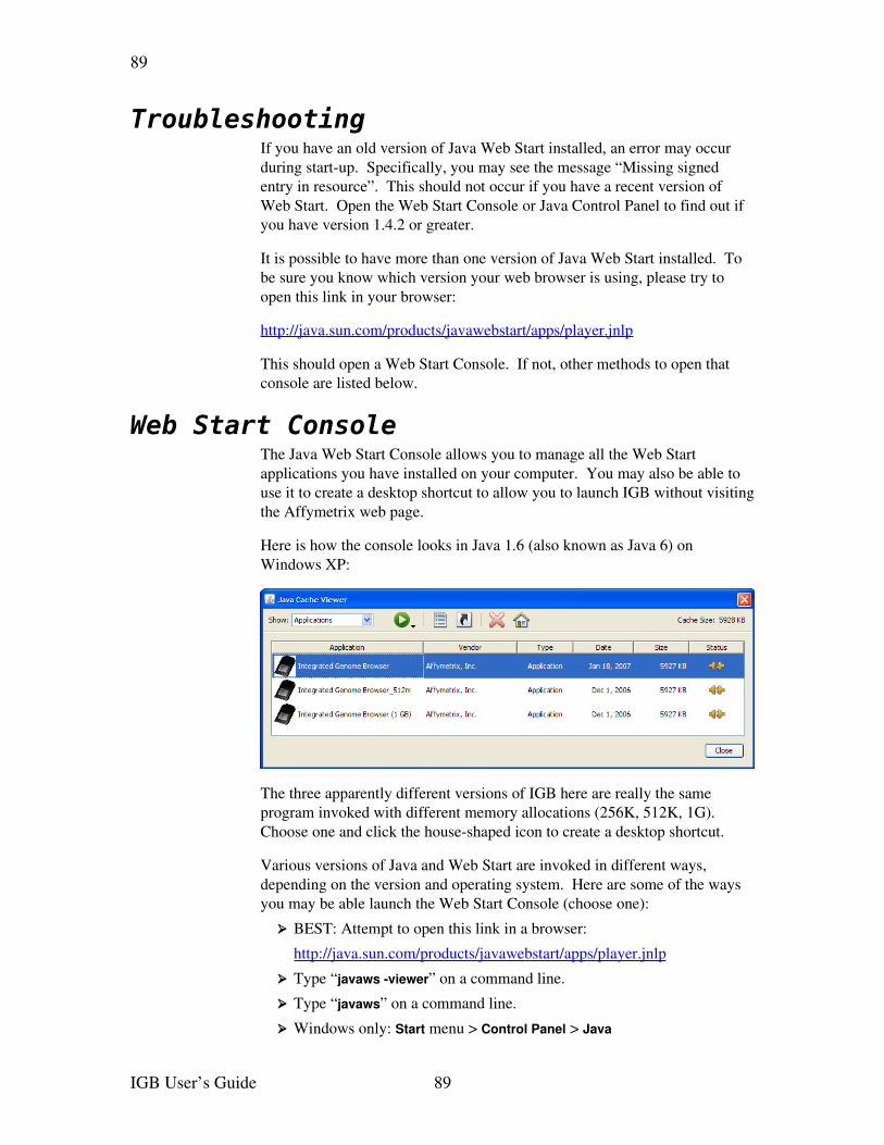
89
TroubleshootingIf you have an old version of Java Web Start installed, an error may occur during startup. Specifically, you may see the message “Missing signed entry in resource”. This should not occur if you have a recent version of Web Start. Open the Web Start Console or Java Control Panel to find out if you have version 1.4.2 or greater.
It is possible to have more than one version of Java Web Start installed. To be sure you know which version your web browser is using, please try to open this link in your browser:
http://java.sun.com/products/javawebstart/apps/player.jnlp
This should open a Web Start Console. If not, other methods to open that console are listed below.
Web Start ConsoleThe Java Web Start Console allows you to manage all the Web Start applications you have installed on your computer. You may also be able to use it to create a desktop shortcut to allow you to launch IGB without visiting the Affymetrix web page.
Here is how the console looks in Java 1.6 (also known as Java 6) on Windows XP:
The three apparently different versions of IGB here are really the same program invoked with different memory allocations (256K, 512K, 1G). Choose one and click the houseshaped icon to create a desktop shortcut.
Various versions of Java and Web Start are invoked in different ways, depending on the version and operating system. Here are some of the ways you may be able launch the Web Start Console (choose one):
➢ BEST: Attempt to open this link in a browser:
http://java.sun.com/products/javawebstart/apps/player.jnlp
➢ Type “javaws viewer” on a command line.
➢ Type “javaws” on a command line.
➢ Windows only: Start menu > Control Panel > Java
IGB User’s Guide 89
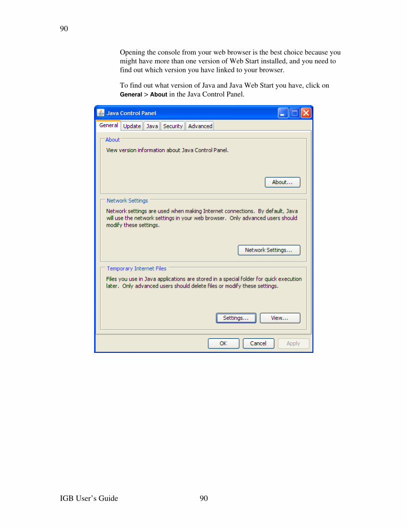
90
Opening the console from your web browser is the best choice because you might have more than one version of Web Start installed, and you need to find out which version you have linked to your browser.
To find out what version of Java and Java Web Start you have, click on General > About in the Java Control Panel.
IGB User’s Guide 90
91
Appendix 2 Troubleshooting
If you have problems, first doublecheck the instructions for the specific task you’re working on, and then try solutions below that are specific to the area of IGB you’re working on, and finally try the general troubleshooting items at the end of this appendix.
Troubleshooting specific areasBelow are troubleshooting tips for some areas of IGB.
IGB seems slow or sluggishTry the following:
➢ Delete any graphs you don't need.
➢ Hide any annotation tracks you don't need.
➢ Turn off slicing: See Slicing on page 44. Or make sure the Slicing tabbed panel is closed.
➢ Turn off graph thresholding if you are not actively using it.
➢ Turn off the gene id labels for all tracks.
➢ Turn off colorbyscore in all annotation tracks.
➢ Experiment with different graph styles. Some styles draw faster than others.
➢ Launch IGB using a larger RAM memory allocation. See Typicalinstallation using Java Web Start on page 9.
Keyboard shortcut command doesn’t workYou may have changed the shortcut key in the preferences. See Changingkeyboard commands on page 98. Note that after changing the shortcut keys, you must close and relaunch IGB before the changes will take effect.
Alternatively some component other than the viewer window may have the “keyboard focus”. For example, your key strokes may be going to a text entry box or to another application. Click anywhere in the viewer to return the keyboard focus to it.
Keyboard shortcuts for scrolling and zooming may behave unexpectedly if the main view and the slice view are open in the same window. Try closing the slice view or moving it to a separate window.
IGB User’s Guide 91
92
Out of memory errorsIf you are working with many graphs or sequences, you may run out of memory. These errors are most likely to occur during file parsing, but sometimes occur at other times. After you receive an outofmemory error, most functions will become unusable and you will have to close and relaunch IGB.
You may need to launch IGB using a larger RAM memory allocation. See Typical installation using Java Web Start on page 9.
The ratio of memory used to memory available is shown in the status bar. See The status bar on page 14.
Tab or tab window is missingIf you have opened a tab in a new window, the tab window may have become hidden behind the main IGB window or another window. Each operating system has ways to help you locate and navigate between all open windows. On the Windows operating system, the combination of <Alt> and <Tab> keys often works to cycle through all open windows.
Tier labels don't line-up with tiersFrom time to time, it is possible that the tier labels on the lefthand side of the main view will not lineup vertically with the tiers in the main view. If this happens, simply drag the border between the labels and the tiers to the left or right to resize the tier labels. They should snap back into alignment.
You can't see all the tiersYou may need to zoomin vertically. See Zooming and scrolling vertically on page 18. Or you may have hidden some tiers manually. See Hiding andshowing annotation tracks and Hiding and showing strands on page 40.
Reverse strand data appears above the axisBy default, IGB places reverse strand data below the coordinates axis and positive strand data above the axis. But if you have rearranged any of the tiers, it is possible that reverse strand tiers will endup above the axis. We may change IGB in future to make this situation impossible, but there is currently nothing preventing this from happening. If you want to put the reverse strands below the axis, you can move them there manually. See Reordering tracks toptobottom on page 39.
General troubleshootingIf anything you’re working on doesn’t work, try these common fixes, even if they don’t seem intuitive:
➢ Read the section in this document related to the task you are trying to accomplish.
IGB User’s Guide 92

93
➢ Load sequence residues for the chromosome or file you’re using.
➢ Make sure the genome version and chromosome in the viewer match those of whatever you’re trying to load or compare.
➢ Make sure you’ve selected the gene, not the exon, or viceversa.
➢ Unclamp the view. See Clamping on a view on page 82.
➢ Try limiting the region in the viewer to less than 2 million bases when loading data from DAS servers.
➢ Make sure you’re connected to the network and the server or data source that you’re connecting to is up and running.
➢ Make sure you haven’t hidden any tracks or graphs.
➢ Open the console and look for error or warning messages. See Theconsole on page 17.
IGB User’s Guide 93
94
Appendix 3 Preferences
The preferences window contains a set of tabbed panels allowing you to set preferences for various aspects of the program. Open the preferences window by choosing File menu > Preferences.
You can set preferences for the following:
➢ Appearance of the viewer, tracks, annotations, and graphs
➢ Locations of data sources
➢ Keyboard commands for tasks that you perform frequently
➢ Appearance and function of specific features.
Most preferences, such as settings for tier properties, apply immediately to data that is already loaded. while others, such as default settings for graphs, apply only to future activity. A small number of preference changes, such as changing keyboard shortcuts, require that you close and relaunch IGB.
Preference settings will remain in effect after you shut down and relaunch IGB. You can also export and import these preferences in an XML file.
There is some documentation for specific preferences included inside the program. To view the Help, choose File menu > Preferences, then choose an option from the Help menu in the Preferences dialog box The documentation inside the program may be more recent or more complete than this document.
Importing and exporting preferencesYou can set each preference manually, or you can export and import preferences to an XML file to save them or share them among a group of people who are working on similar or related projects. This is also useful if you want to move IGB from one computer to another. Affymetrix may also provide preferences files to optimize IGB for analyzing certain data sets.
The XML file used for preference export and import, is not intended to be edited by hand and we provide no documentation on its format.
Note: In earlier versions of IGB, preferences were set by the user by editing a file called “igb_prefs.xml”. That file is being deprecated, though it is still used by some users for some advanced functions.
Exporting preference settingsYou can export preference settings for use in different instances of IGB or to share with other IGB users.
➢ Choose File menu > Preferences.
IGB User’s Guide 94
95
➢ In the Preferences dialog box, choose Preferences menu > Export Preferences.
➢ Choose the destination and filename to which you want to save your preference settings.
➢ Click Save.
Importing preference settingsYou can import preference settings that you, Affymetrix, or another IGB user has exported using the procedure above. You can freely exchange preferences between Windows, Linux, and Macintosh systems.
Preferences in the file that you import are merged with your existing preferences.
➢ WARNING: be sure you trust the provider of the file.
➢ Choose File menu > Preferences.
➢ In the Preferences dialog box, choose Preferences menu > Import Preferences.
➢ Choose the saved preferences file and click Open.
Customizing the default appearance of tracks
You can customize the way an annotation type looks in the track.
For most annotation types, IGB remembers your settings so that the annotation type appears the same way each time you load it.
IGB does not remember settings for graphs and for temporary data resulting from arithmetic manipulations, such as intersections and unions of tracks.
You can set default values for most of track parameters so that all annotation types display by default using settings that you specify.
Your settings apply to both forward and reverse strands.
Some of these settings can also be made in the menu that is shown when you rightclick the name of the annotation type in the Tracks panel. The effect is the same.
To customize the appearance of a track:
➢ Load the annotation type(s) to customize.
➢ Select File menu > Preferences > Tiers. Or Rightclick on the track name in the Tracks panel and choose Customize.
➢ In the Preferences dialog box, make selections for the annotation type(s) to customize, following instructions in the sections that follow.
➢ If the name of the track is shown in italic font, the settings for that track will apply only to the current session. (This is the case for
IGB User’s Guide 95
96
certain tracks that were created through manipulations such as intersections or unions of other tracks.)
➢ If the track name is shown in normal font, the settings will be used for future sessions.
➢ The track labeled “default” will apply to any new track loaded in the future for which you have not already made customizations.
➢ When finished setting preferences, close the Preferences dialog box.
The check box labeled Auto Refresh determines whether your changes are applied as you make them or only when you close the Preferences dialog box. If you have loaded a large number of annotations and the screen takes a long time to draw, you should turn Auto Refresh off.
Changing the name of the trackYou can change the label of the data set as it appears in the tracks panel.
➢ Doubleclick the cell in the Display Name column. Your cursor will blink in the field.
➢ Type the name you want to use. Leave this field blank if you want to use the default name for this track.
➢ Press the <Enter> key.
Changing the color of annotations➢ Click the color that is showing in the Color column.
➢ Click a color in the palette.
➢ Click OK.
Changing the background color of the track➢ Click the color that is showing in the Background column.
➢ Click a color in the palette.
➢ Click OK.
Displaying both strands in one track or twoTo display forward and reverse strands in two tracks (+) and ():
➢ Click the checkbox in the 2 Tracks column to add a check mark.
To display both strands in one track (+/):
➢ Click the checkbox in the 2 Tracks column to remove the check mark.
There is also a global setting to choose to display or not to display each strand by accessing the View > Strands menu.
Collapsing annotation rows into a single rowTo always display the data set with all annotation rows collapsed into the minimum height for the data set:
IGB User’s Guide 96
97
➢ Click the checkbox in the Collapsed column to add a check mark.
To display all annotation rows in the data set:
➢ Click the checkbox in the Collapsed column to remove the check mark.
Setting the maximum number of annotation rows to display
You can specify the maximum number of annotation rows to display when the annotation track is not collapsed:
➢ Doubleclick the cell in the Max Depth column. Your cursor will blink in the field.
➢ Type the maximum number of annotation rows to display. A suggested value is 5. A value of 0 indicates that there is no limit on the number of rows to display.
➢ Press the <Enter> key.
To cancel a restricted maximum that you have set:
➢ Doubleclick the cell in the Max Depth column. Your cursor will blink in the field.
➢ Clear the value in the field or set it to zero.
➢ Press the <Enter> key.
Grouping exonsThis preference determines whether to connect groups of exons into transcripts.
For data with no intronexon structure, such as repeats or contigs, exons should not be connected. For items that do have intronexon structure, not connecting the exons may affect whether labels are displayed.
Almost all of the data types used in IGB should leave this setting with the default value of true.
To display annotations in the data track with exons connected or not connected:
➢ Click the checkbox in the Connected column to add or remove a check mark.
Choosing annotation id labelsEach annotation track can display id labels next to the annotations. You can hide annotation id labels or show them using any property type that is available for that data set. For example, RefSeq annotations have both an “id” and a “gene name” property. You can choose to display either of these as an id label.
IGB User’s Guide 97
98
You can also choose to turn off labels. IGB will require less memory to run and will draw the display faster when labels are turned off.
To see what label options are available for the data set that you are customizing, click an annotation in the browser window, then click the Selection Info tab. Look at the properties listed in the property column. The most typical property names that will be useful for labels are “id” and “gene name”, but some annotation types have other properties that might make good labels.
➢ Doubleclick the cell in the Label field column. Your cursor will blink in the field.
➢ Type the name of the source for annotation labels:
➢ “id” Most data sets include “id” values.
➢ To display no label, leave the field blank. This reduces the memory that IGB requires to run, and speeds drawing of the display.
➢ Other property names, if they appear in the Selection Info tab. Enter them as they appear in Selection Info. For example, “gene name” is a possible choice for RefSeq transcripts and “source” is a possible choice for data from GFF files.
➢ Press the <Enter> key.
Note: Exons and whole transcripts usually have different sets of properties. If you have chosen to display exons without connection lines, labels will only be visible if the individual exons have the property that you specify.
Changing keyboard commandsYou can set keyboard shortcuts for many menu and other functions. The list of functions for which you can set keyboard shortcuts appears in the Preferences described in the following procedure.
To set or change keyboard commands:
➢ Choose File menu > Preferences.
➢ Click the Shortcuts tab.
➢ Click the action for which you want to establish a keyboard command.
➢ Click in the field labeled Type a shortcut for <the command you selected>.
➢ Press the keys that you want to assign to the function you selected, for example, CtrlShiftX. You cannot use keystrokes that your operating system uses, such as CtrlAltDelete on Windows. If you make a mistake, simply type the keystroke(s) that you want, and the new keystrokes will replace the erroneous keystrokes that you entered.
➢ Click the Apply this shortcut button.
➢ Your new keyboard shortcut(s) will be available after you close and relaunch IGB.
IGB User’s Guide 98
99
To clear keyboard commands:
➢ Click the shortcut from which you want to remove the command.
➢ Click Clear this shortcut.
➢ Your changes take affect after you close and then relaunch IGB.
Some action names may appear that don't seem to have any function. This could happen if you have installed and then uninstalled some plugins, or if some actions have been renamed.
Keyboard Shortcut keys for zooming and scrolling the view will apply both in the main view and in the sliced view. The effect can be confusing when both views are visible in the same window at the same time. Opening the sliced view in a separate window can give more predictable shortcut behavior.
Setting graph preferencesYou can set preferences for the way graphs display in the viewer window.
Changes affect graphs that you load after you complete the procedure below.
To change default characteristics of graphs:
➢ Choose File menu > Preferences.
➢ Click the Graphs tab.
➢ Choose options for the following:
➢ Whether graphs float or are attached to tracks.
➢ Whether the complete URL should be used as the file label (typically false).
➢ Whether to create graphs from data in “.egr” files (typically true).
When importing .egr files, the genomic locations will be shown as rectangular blocks. Check this check box to additionally display the score data in graph format.
➢ The default colors to use for heatmap graphs.
➢ If you are finished setting preferences, close the Preferences dialog box.
Setting color and axis display preferences
Miscellaneous options are grouped together in the Preferences tab labeled Other Options. These include color and display properties for the axis, edge matching, ORF analysis, and other things.
To access these options:
IGB User’s Guide 99
100
➢ Choose File menu > Preferences.
➢ Click the Other Options tab.
Setting axis display – option descriptionsYou can set the following preferences for the appearance of the coordinate axis track that runs horizontally across the center of the viewer window:
➢ Background
➢ Foreground
➢ Number format
➢ Full displays like: 20000kb
➢ Comma displays like: 20,000,000
➢ Abbrev displays like: 20M
Setting ORF and stop-codon colorsBy default, ORFs (Open Reading Frames) are indicated in the sliced view with green and stop codons are indicated in pink
➢ To change the stop codon color, click the button beside Stop Codon.
➢ To change the ORF color, click the button beside Dynamic ORF.
➢ Click a color in the palette.
➢ Click OK.
Setting other optionsOther options you can set:
Option Description
Ask before exiting Whether IGB asks you to confirm that you really want to exit when you choose File menu > Exit or click the [X] in the title bar.
Keep hairline in view Whether to automatically prevent the hairline from moving outside the view as you scroll. (Recommended true).
Browser Command Command used to launch a browser (e.g., “/usr/bin/firefox').
➢ Check the check boxes beside the options you want to enable.
IGB User’s Guide 100

101
License
Source code for IGB is released under the Common Public License, v1.0, an OSI approved open source license. IGB uses other open source software packages that are not distributed with the IGB source code release, including Xerces and Jetspeed from Apache, and Jetty from Mortbay Consulting, which are covered by their own open source licenses. IGB is Copyright (c) 20002007 Affymetrix, Inc. Research and development of IGB is supported in part by NIH grant R01HG003040.
Common Public License Version 1.0
THE ACCOMPANYING PROGRAM IS PROVIDED UNDER THE TERMS OF THIS COMMON PUBLIC LICENSE ("AGREEMENT"). ANY USE, REPRODUCTION OR DISTRIBUTION OF THE PROGRAM CONSTITUTES RECIPIENT'S ACCEPTANCE OF THIS AGREEMENT.
1. DEFINITIONS
"Contribution" means:
a) in the case of the initial Contributor, the initial code and documentation distributed under this Agreement, and
b) in the case of each subsequent Contributor:
i) changes to the Program, and
ii) additions to the Program;
where such changes and/or additions to the Program originate from and are distributed by that particular Contributor. A Contribution 'originates' from a Contributor if it was added to the Program by such Contributor itself or anyone acting on such Contributor's behalf. Contributions do not include additions to the Program which: (i) are separate modules of software distributed in conjunction with the Program under their own license agreement, and (ii) are not derivative works of the Program.
"Contributor" means any person or entity that distributes the Program.
"Licensed Patents " mean patent claims licensable by a Contributor which are necessarily infringed by the use or sale of its Contribution alone or when combined with the Program.
"Program" means the Contributions distributed in accordance with this Agreement.
"Recipient" means anyone who receives the Program under this Agreement, including all Contributors.
2. GRANT OF RIGHTS
a) Subject to the terms of this Agreement, each Contributor hereby grants Recipient a nonexclusive, worldwide, royaltyfree copyright license to reproduce, prepare derivative works of, publicly display, publicly perform, distribute and sublicense the Contribution of such Contributor, if any, and such derivative works, in source code and object code form.
IGB User’s Guide 101

102
b) Subject to the terms of this Agreement, each Contributor hereby grants Recipient a nonexclusive, worldwide, royaltyfree patent license under Licensed Patents to make, use, sell, offer to sell, import and otherwise transfer the Contribution of such Contributor, if any, in source code and object code form. This patent license shall apply to the combination of the Contribution and the Program if, at the time the Contribution is added by the Contributor, such addition of the Contribution causes such combination to be covered by the Licensed Patents. The patent license shall not apply to any other combinations which include the Contribution. No hardware per se is licensed hereunder.
c) Recipient understands that although each Contributor grants the licenses to its Contributions set forth herein, no assurances are provided by any Contributor that the Program does not infringe the patent or other intellectual property rights of any other entity. Each Contributor disclaims any liability to Recipient for claims brought by any other entity based on infringement of intellectual property rights or otherwise. As a condition to exercising the rights and licenses granted hereunder, each Recipient hereby assumes sole responsibility to secure any other intellectual property rights needed, if any. For example, if a third party patent license is required to allow Recipient to distribute the Program, it is Recipient's responsibility to acquire that license before distributing the Program.
d) Each Contributor represents that to its knowledge it has sufficient copyright rights in its Contribution, if any, to grant the copyright license set forth in this Agreement.
3. REQUIREMENTS
A Contributor may choose to distribute the Program in object code form under its own license agreement, provided that:
a) it complies with the terms and conditions of this Agreement; and
b) its license agreement:
i) effectively disclaims on behalf of all Contributors all warranties and conditions, express and implied, including warranties or conditions of title and noninfringement, and implied warranties or conditions of merchantability and fitness for a particular purpose;
ii) effectively excludes on behalf of all Contributors all liability for damages, including direct, indirect, special, incidental and consequential damages, such as lost profits;
iii) states that any provisions which differ from this Agreement are offered by that Contributor alone and not by any other party; and
iv) states that source code for the Program is available from such Contributor, and informs licensees how to obtain it in a reasonable manner on or through a medium customarily used for software exchange.
When the Program is made available in source code form:
a) it must be made available under this Agreement; and
b) a copy of this Agreement must be included with each copy of the Program.
Contributors may not remove or alter any copyright notices contained within the Program.
Each Contributor must identify itself as the originator of its Contribution, if any, in a manner that reasonably allows subsequent Recipients to identify the originator of the Contribution.
IGB User’s Guide 102

103
4. COMMERCIAL DISTRIBUTION
Commercial distributors of software may accept certain responsibilities with respect to end users, business partners and the like. While this license is intended to facilitate the commercial use of the Program, the Contributor who includes the Program in a commercial product offering should do so in a manner which does not create potential liability for other Contributors. Therefore, if a Contributor includes the Program in a commercial product offering, such Contributor ("Commercial Contributor") hereby agrees to defend and indemnify every other Contributor ("Indemnified Contributor") against any losses, damages and costs (collectively "Losses") arising from claims, lawsuits and other legal actions brought by a third party against the Indemnified Contributor to the extent caused by the acts or omissions of such Commercial Contributor in connection with its distribution of the Program in a commercial product offering. The obligations in this section do not apply to any claims or Losses relating to any actual or alleged intellectual property infringement. In order to qualify, an Indemnified Contributor must: a) promptly notify the Commercial Contributor in writing of such claim, and b) allow the Commercial Contributor to control, and cooperate with the Commercial Contributor in, the defense and any related settlement negotiations. The Indemnified Contributor may participate in any such claim at its own expense.
For example, a Contributor might include the Program in a commercial product offering, Product X. That Contributor is then a Commercial Contributor. If that Commercial Contributor then makes performance claims, or offers warranties related to Product X, those performance claims and warranties are such Commercial Contributor's responsibility alone. Under this section, the Commercial Contributor would have to defend claims against the other Contributors related to those performance claims and warranties, and if a court requires any other Contributor to pay any damages as a result, the Commercial Contributor must pay those damages.
5. NO WARRANTY
EXCEPT AS EXPRESSLY SET FORTH IN THIS AGREEMENT, THE PROGRAM IS PROVIDED ON AN "AS IS" BASIS, WITHOUT WARRANTIES OR CONDITIONS OF ANY KIND, EITHER EXPRESS OR IMPLIED INCLUDING, WITHOUT LIMITATION, ANY WARRANTIES OR CONDITIONS OF TITLE, NONINFRINGEMENT, MERCHANTABILITY OR FITNESS FOR A PARTICULAR PURPOSE. Each Recipient is solely responsible for determining the appropriateness of using and distributing the Program and assumes all risks associated with its exercise of rights under this Agreement, including but not limited to the risks and costs of program errors, compliance with applicable laws, damage to or loss of data, programs or equipment, and unavailability or interruption of operations.
6. DISCLAIMER OF LIABILITY
EXCEPT AS EXPRESSLY SET FORTH IN THIS AGREEMENT, NEITHER RECIPIENT NOR ANY CONTRIBUTORS SHALL HAVE ANY LIABILITY FOR ANY DIRECT, INDIRECT, INCIDENTAL, SPECIAL, EXEMPLARY, OR CONSEQUENTIAL DAMAGES (INCLUDING WITHOUT LIMITATION LOST PROFITS), HOWEVER CAUSED AND ON ANY THEORY OF LIABILITY, WHETHER IN CONTRACT, STRICT LIABILITY, OR TORT (INCLUDING NEGLIGENCE OR OTHERWISE) ARISING IN ANY WAY OUT OF THE USE OR DISTRIBUTION OF THE PROGRAM OR THE EXERCISE OF ANY RIGHTS GRANTED HEREUNDER, EVEN IF ADVISED OF THE POSSIBILITY OF SUCH DAMAGES.
7. GENERAL
If any provision of this Agreement is invalid or unenforceable under applicable law, it shall not affect the validity or enforceability of the remainder of the terms of this Agreement, and without further action by the parties hereto, such provision shall be reformed to the minimum extent necessary to make such provision valid and enforceable.
If Recipient institutes patent litigation against a Contributor with respect to a patent applicable to software (including a crossclaim or counterclaim in a lawsuit), then any patent licenses granted by that Contributor to
IGB User’s Guide 103

104
such Recipient under this Agreement shall terminate as of the date such litigation is filed. In addition, if Recipient institutes patent litigation against any entity (including a crossclaim or counterclaim in a lawsuit) alleging that the Program itself (excluding combinations of the Program with other software or hardware) infringes such Recipient's patent(s), then such Recipient's rights granted under Section 2(b) shall terminate as of the date such litigation is filed.
All Recipient's rights under this Agreement shall terminate if it fails to comply with any of the material terms or conditions of this Agreement and does not cure such failure in a reasonable period of time after becoming aware of such noncompliance. If all Recipient's rights under this Agreement terminate, Recipient agrees to cease use and distribution of the Program as soon as reasonably practicable. However, Recipient's obligations under this Agreement and any licenses granted by Recipient relating to the Program shall continue and survive.
Everyone is permitted to copy and distribute copies of this Agreement, but in order to avoid inconsistency the Agreement is copyrighted and may only be modified in the following manner. The Agreement Steward reserves the right to publish new versions (including revisions) of this Agreement from time to time. No one other than the Agreement Steward has the right to modify this Agreement. IBM is the initial Agreement Steward. IBM may assign the responsibility to serve as the Agreement Steward to a suitable separate entity. Each new version of the Agreement will be given a distinguishing version number. The Program (including Contributions) may always be distributed subject to the version of the Agreement under which it was received. In addition, after a new version of the Agreement is published, Contributor may elect to distribute the Program (including its Contributions) under the new version. Except as expressly stated in Sections 2(a) and 2(b) above, Recipient receives no rights or licenses to the intellectual property of any Contributor under this Agreement, whether expressly, by implication, estoppel or otherwise. All rights in the Program not expressly granted under this Agreement are reserved.
This Agreement is governed by the laws of the State of New York and the intellectual property laws of the United States of America. No party to this Agreement will bring a legal action under this Agreement more than one year after the cause of action arose. Each party waives its rights to a jury trial in any resulting litigation.
IGB User’s Guide 104
105
Index
Alternate splicing............................41, 42Analyze ORFs checkbox.......................84Annotation tracks............................13, 35
Changing background color of..........96Changing color of........................37, 96Changing names of......................37, 96Collapsing...................................38, 96Customizing......................................35Deleting.............................................37Expanding.........................................38Hiding................................................37Id labels.......................................39, 97Max expand.......................................39Reordering.........................................36Saving................................................66Selecting............................................36Setting maximum rows...............38, 96Showing hidden.................................37Summarizing.....................................43
Annotations...........................................11Cache.................................................81Comparing.............................41, 43, 45Density of coverage..........................44Finding........................................16, 32Id labels.................................35, 40, 97Scores................................................40Selecting............................................19Sources..................................23, 24, 79
Ask before exiting...............................100Bar graphs.............................................51Blat mapping.........................................73Bookmarks................................................
Creating.............................................76Editing...............................................76Exporting...........................................77Importing...........................................77Using.................................................76
Cache...............................................23, 81Chromosome.........................................11Clamp to view...........................19, 82, 93
Clear All................................................19CNAT..............................................22, 48Combine Selected Tracks......................46Console..................................................16Contigs......................................14, 23, 83Coordinates track......................29, 30, 33
In sliced view....................................42Setting preferences............................99
Copy and paste..........................................Sequence.....................................31, 75Table cells.........................................77
Cytobands........................................14, 23DAS.......................................................24DAS/1....................................................24DAS/2....................................................24Data Access tab.....................................22Data sources..............................................
Configuring.......................................79DAS...................................................24Files...................................................25QuickLoad.........................................23
Deletions...............................................42Density of annotations..........................44Desktop shortcut...................................89Documentation........................................8Dot graphs.............................................51Edge matching.......................................41
Adjust match fuzziness.....................41Setting colors.....................................41
Ensemble...............................................28EnsGene................................................28ESTs....................................17, 48, 52, 66ExACT............................................22, 48Exons.........................................................
Connecting or not connecting...........97File formats...........................................26
Annotation formats...........................27Bar.....................................................49Bed....................................................27
IGB User’s Guide 105
106
Bnib.............................................29, 30Chp....................................................49Compressed.......................................27Egr.....................................................49Gff.....................................................27GFF3.................................................27Gr......................................................49Graph formats...................................49Gtf.....................................................27Psl......................................................27Sequence formats..............................30Sgr.....................................................49Wig....................................................49
File formats,..........................................49Files...........................................................
Compressed.......................................27Extension...........................................27Graph.................................................67Loading.............................................26Merging.............................................26
Finding......................................................Annotations.......................................32Sequences..........................................33
GCOS..............................................22, 48Genome.....................................11, 26, 93Genome.....................................................
Definition..........................................11In title bar..........................................13Synonyms..........................................80
GenoViz..................................................8Get more info..................................28, 73Graph styles...........................................51Graph tracks....................................50, 59Graphs.......................................12, 48, 92
Adjusting...........................................50Arithmetic functions.........................61Attached............................................59Color..................................................57Comparing.........................................61Deleting.......................................58, 60Details...............................................67Duplicating........................................60Floating.......................................50, 59Graph handle.........................19, 50, 59
Height................................................50In sliced view....................................42Interval graphs...................................48Labeling............................................59Nonlinear scale................................60Position graphs..................................48Printing..............................................67Saving................................................66Scale............................................57, 66Selecting......................................19, 50Setting preferences............................98Styles.................................................51Thresholds.............................62, 66, 76Visible bounds.............................58, 66Yaxis................................................59
Hairline..................................................15Heat map graphs....................................52IGB............................................................
Current version....................................9Desktop shortcut...............................89Installing IGB......................................9Launching..........................................10Main window....................................12Searching in.......................................32
Insertions...............................................42Installing IGB..........................................9Java..........................................................9
Installation...........................................9Version................................................9Web Start Console............................89
Javaws...................................................89Keyboard commands...........21, 42, 91, 98Launching IGB......................................10
Multiple instances.............................10Line graphs............................................51Macintosh............................................8, 9Make annotation coverage track...........44Make annotation depth track.................44Max gap.....................................................
Thresholds.........................................65Merge with currently loaded data.........26Min run......................................................
Thresholds.........................................65Min/Max/Avg graphs............................51
IGB User’s Guide 106
107
Multiple instances of IGB.....................10Navigating.................................................
To annotation....................................32To coordinate....................................18
Navigation.............................................16NCBI.....................................................28NetAffx.................................................70Offsets.......................................................
Thresholds.........................................65Open File...............................................26ORFs.........................................................
Setting colors.....................................99Out of memory errors............................92PolyA site..............................................73PolyA stack...........................................73Polyadenylation sites.............................73Preferences............................................94
Exporting...........................................94Importing...........................................95
Printing..................................................77Probe sets..................................................
Files...................................................70Visualizing........................................69
Query sequence.........................................In psl files..........................................27
QuickLoad.............................................23Advanced features.............................79
Range box.............................................18RefSeq annotations...................22, 23, 28Scroll bars.............................................15Scrolling..........................................15, 17
Autoscroll........................................17Restricting.........................................82
Select parent..........................................19Selecting....................................................
Annotations.................................19, 93Graphs.........................................19, 50Sequence residues.............................20
Sequence...................................................Copy and paste..................................75Selecting............................................20
Sequence residues................23, 2931, 92Sequences..............................................12
Cache.................................................23
Copy and paste..................................31Finding..............................................32Selecting............................................19Wildcard searches.............................33
Shortcuts................................................98Shrinkwrapping....................................83Slice Buffer...........................................43Slice By Selection.................................42Slicing.................................41, 66, 84, 91Source code.........................................8, 9Stairstep graphs.....................................52Status bar...............................................13Strands...................................................37
Displaying both or one......................96Forward strand..................................37Mixed strand.....................................37Reverse strand...................................37
Summarizing.............................................Annotation tracks..............................43
System requirements...............................9Tabbed panels...........................15, 20, 92Tabbed panels...........................................
Data Access.................................16, 29Graph Adjuster..................................50Pattern Search..............................3234Selection Info..............................27, 67Sliced view..................................42, 74
Target sequence.........................................In psl files..........................................27
Thresholding.............................63, 66, 91Tiling arrays..............................22, 48, 65Title bar.................................................12Toggle Shrink Wrapping.......................83Track handles..................................14, 35Track lines.................................27, 85, 86Tracks....................................................13
Combining.........................................45Graph threshold.................................66Zooming vertically............................17
Tracks panel..............................................Resizing.............................................35
Translation frames.................................84UCSC....................................................28
DAS server........................................24
IGB User’s Guide 107
108
UCSC genome browser...............75, 85Unsequenced regions............................31Untranslated regions.............................14UseScore...............................................40UTRs.....................................................14Viewer...................................................13Zoom sliders..........................................15Zooming................................................17
Horizontal zoom slider......................17In sliced view....................................42Vertical zoom slider..........................17
IGB User’s Guide 108