Integrated flight/thrust vectoring control for jet-poweredunmanned aerial vehicles with ACHEON propulsion

Item type Article

Authors Cen, Zhaohui; Smith, Tim; Stewart, Paul; Stewart, Jill

Citation Cen, Z. et al (2014) 'Integrated flight/thrust vectoringcontrol for jet-powered unmanned aerial vehicles withACHEON propulsion', Proceedings of the Institution ofMechanical Engineers, Part G: Journal of AerospaceEngineering, 229 (6):1057. DOI:10.1177/0954410014544179

DOI 10.1177/0954410014544179

Journal Proceedings of the Institution of Mechanical Engineers,Part G: Journal of Aerospace Engineering

Rights Archived with thanks to Proceedings of the Institution ofMechanical Engineers, Part G: Journal of AerospaceEngineering

Downloaded 12-May-2018 02:41:37

Item License http://creativecommons.org/licenses/by/4.0/

Link to item http://hdl.handle.net/10545/609450

Seediscussions,stats,andauthorprofilesforthispublicationat:https://www.researchgate.net/publication/274994011

Integratedflight/thrustvectoringcontrolforjet-poweredunmannedaerialvehicleswithACHEONpropulsion

ArticleinProceedingsoftheInstitutionofMechanicalEngineersPartGJournalofAerospaceEngineering·April2014

ImpactFactor:0.68·DOI:10.1177/0954410014544179

CITATIONS

2

READS

78

4authors,including:

ZhaohuiCen

QatarFoundation

19PUBLICATIONS48CITATIONS

SEEPROFILE

PaulStewart

UniversityofDerby

63PUBLICATIONS257CITATIONS

SEEPROFILE

JillStewart

SheffieldHallamUniversity

25PUBLICATIONS68CITATIONS

SEEPROFILE

Allin-textreferencesunderlinedinbluearelinkedtopublicationsonResearchGate,

lettingyouaccessandreadthemimmediately.

Availablefrom:PaulStewart

Retrievedon:09May2016

1

1. INTRODUCTION

Thrust vector nozzles are increasing interest in modern combat aircraft applications. This is due to the requirement to enhance the maneuverability of the aircraft on the one hand without excessively increasing the need for exotic (high strength) vector nozzle materials. Vector nozzles have been tested on many experimental airplanes such as F-18/HARV, X-31, F-15 ACTIVE and F-16 VISTA and they have been flying on Su-30 MKI, F-22, JSF MIG-29 OVT [1-5] and F-35 A/B/C. For Unmanned Aerial Vehicles (UAV), vector nozzles have more practical applications than traditional aircraft because it can significantly improve the maneuverability without the human limitation of the pilot impacting operation performance [6-7] .

Generally, three types of vector nozzles are used for thrust–vectoring propulsion: mechanical nozzle manipulation; secondary fluidic injection; exhaust flow deflection [2-4, 8-9]. As a result of the need to continuously perform moving actions of the control surfaces the mechanical nozzle ages and is subject to fatigue reducing reliability and useful life.

Secondary fluidic injection and exhaust flow deflection, which are both fluidic thrust vector techniques, do not require mechanical moving parts that are subjected to the same mechanical stresses, but are limited by the range of deflection angle available and are difficult to precisely control. Therefore, the two fluidic thrust-vectoring control techniques are also difficult to apply in fixed-wing jet UAV’s because of the performance boundary.

The ACHEON project is a novel propulsion concept which aims to produce radically new aircraft propulsion systems (and possibly aircraft). It aims to verify a novel propulsion system with thrust vectoring capabilities formally named HOMER (High-speed Orienting Momentum with Enhanced Reversibility) and recently patented by the University of Modena and Reggio Emilia in Italy, together with a smart and effective active control system based on PEACE (Plasma Enhanced Actuator for Coanda Effect) a study by the Universidad de Beira Interior in Portugal [10-12]. The successful integration of these two new concepts involves solving the way in which high speed streams mix and their interaction with Coanda surfaces such that a vectoring system can be realized which will have a wide spectrum of applications, a precursor to a long-term step advancement in aerial (and naval propulsion and industrial) systems by providing a directionally controllable fluid jet [13]. Because this new nozzle has a wider range of deflection angles and is directionally controllable, it is applicable for fixed-wing jet UAV applications and future super-maneuverable aircraft. Therefore, it is very valuable and important to research the dynamic behavior of this new form of propulsion system and the required integrated flight control methods for robust Thrust Vector (TV) control when applied to all forms of jet aircraft.

The study of Thrust Vectoring Control (TVC) when applied to fixed-wing aircraft and UAVs has increased rapidly in recent years. A number of studies have recently been performed regarding TVC for civil aircraft [14-18], mainly as a means

The present work was performed as part of Project ACHEON with ref. 309041, supported by European Union through the 7th Framework Program. *corresponding author

Integrated Flight/Thrust Vectoring Control for Jet Powered Unmanned Aerial Vehicles with ACHEON Propulsion

Zhaohui Cen1, Tim Smith1, Paul Stewart2*, Jill Stewart3

1. Lincoln School of Engineering, University of Lincoln, Lincoln LN6 7TS, UK 2. School of Engineering, University of Hull, Hull HU6 7RX, UK

3. Faculty of Science and Engineering, University of Chester, Chester CH1 4HJ

E-mail:zcen@lincoln.ac.uk, p.stewart@hull.ac.uk,tismith@lincoln.ac.uk, j.stewart@chester.ac.uk

Abstract: As a new alternative to tilting rotors or turbojet vector mechanical oriented nozzles, ACHEON (Aerial Coanda High Efficiency Orienting-jet Nozzle) has enormous advantages because it is free of moving elements and highly effective for Vertical/Short-Take-Off and Landing (V/STOL) aircraft. In this paper, an integrated flight/ thrust vectoring control scheme for a jet powered Unmanned Aerial Vehicle (UAV) with an ACHEON nozzle is proposed to assess its suitability in jet aircraft flight applications. Firstly, a simplified Thrust-Vectoring (TV) population model is built based on CFD simulation data and parameter identification. Secondly, this TV propulsion model is embedded as a jet actuator for a benchmark fixed-wing ‘Aerosonde’ UAV, and then a four “cascaded-loop” controller, based on nonlinear dynamic inversion (NDI), is designed to individually control the angular rates (in the body frame), attitude angles (in the wind frame), track angles (in the navigation frame), and position (in the earth-centered frame) . Unlike previous research on fixed-wing UAV flight controls or TV controls, our proposed four-cascaded NDI control law can not only coordinate surface control and TV control as well as an optimization controller, but can also implement an absolute self-position control for the autopilot flight control. Finally, flight simulations in a high-fidelity aerodynamic environment are performed to demonstrate the effectiveness and superiority of our proposed control scheme.

Key Words: Thrust-Vectoring, Unmanned Aerial Vehicles, Nonlinear Dynamic Inversion, Integrated Propulsion-based Flight Control

2

of emergency control for use in failure situations. There are also proposals to use TVC combined with the more traditional aerodynamic control surfaces during normal flight. The benefits may be: reduced trim drag (less fuel consumption); reduced aircraft weight; shorter take-off and landing; reduced noise around airfields and improved ability to handle adverse weather and flight conditions. The drawbacks include possible increases in engine weight and complexity. A small number of studies have also been performed using differential thrust to control multi-engine aircraft. This concept is commonly denominated PCA (Propulsion Controlled Aircraft). PCA has mainly been developed as a means to control the aircraft in emergency situations where the traditional aerodynamic control surfaces are lost for some reasons. These concepts have been tested in simulation and in actual flight tests [19].

However, little research has been devoted to the study of TVC to novel jet UAVs. Vinayagam and Sinha [20] have proposed a TVC control strategy for mechanical canted nozzle based jet aircraft-F-18/HARV and have assessed its Velocity Vector Roll (VVR) maneuverability. However, the nozzle has limited deflection angle and it is only suitable for pilot-operated aircraft applications. Yang [21] and Yuhua [22] [15] studied the integrated flight controls for fixed-wing UAV with TV and individually designed the PID control strategy for longitude and latitude control, but it is difficult to decouple the 6-DOF controller channels because of nonlinearities in the fixed-wing aircraft aerodynamics and the limitations of the PID linear control law. It is also especially difficult to implement super-maneuverability flight actions based solely on PID control methods. Bajodah and Hameduddin [16], Wang and Stengel [23] and Lodge and Fielding [24]have conducted research on TVC for fixed-wing UAV’s based on Nonlinear Dynamics Inversion (NDI), but it only included an inner control loop for attitude angular rate control and an outer loop for attitude angle control in the wind-frame; it is therefore not applicable for completely self-positioning control of fixed wing UAV’s utilizing TV.

The contribution of this work consists of proposing an integrated flight/thrust vectoring control scheme for fixed-wing UAVs based on the novel ACHEON propulsion and assess the maneuverability performance of this new configuration. Compared with the latest work on fixed-wing UAV with TV, a novel large-deflection-angle TV nozzle called ACHEON is adopted and a complete self-position control scheme for this type of fixed-wing UAV with TV is developed. Unlike former research work on TVC of fixed-wing aircraft, our control scheme is not only applicable for both remote control and complete self-positioning control, but it is also compatible with three aerodynamic control modes, which includes surface control, TV control, and surface control with TVC. Compared to previous research on maneuverable controller design of fixed-wing aircraft, some special flight conditions such as high-attack angle and velocity vector roll (VVR) are considered and validated based on the proposed aircraft configuration and control scheme, an optimized NDI controller is designed to maximize the maneuverability of the proposed fixed-wing UAV with TV.

This paper is organized as follows. In Section 2, the principle of the ACHEON propulsion model is presented. In section 3, the model of the fixed-wing UAV with TV and the ACHEON nozzle based propulsion model are presented. The proposed integrated control scheme based on NDI is described in Section 4. Section 5 is devoted to the presentation of the simulation results obtained for the flight scenarios when the proposed scheme is applied to the Aerosonde UAV with TV. Finally, conclusions are presented in Section 6.

2. ACHEON PROPULSION SYSTEM MODELLING The AECHEON propulsion system mainly involves two important patented techniques, namely the HOMER nozzle and

PEACE controller. The HOMER nozzle constitutes a novel generation thrust and vectoring jet capability which is designed to overcome the

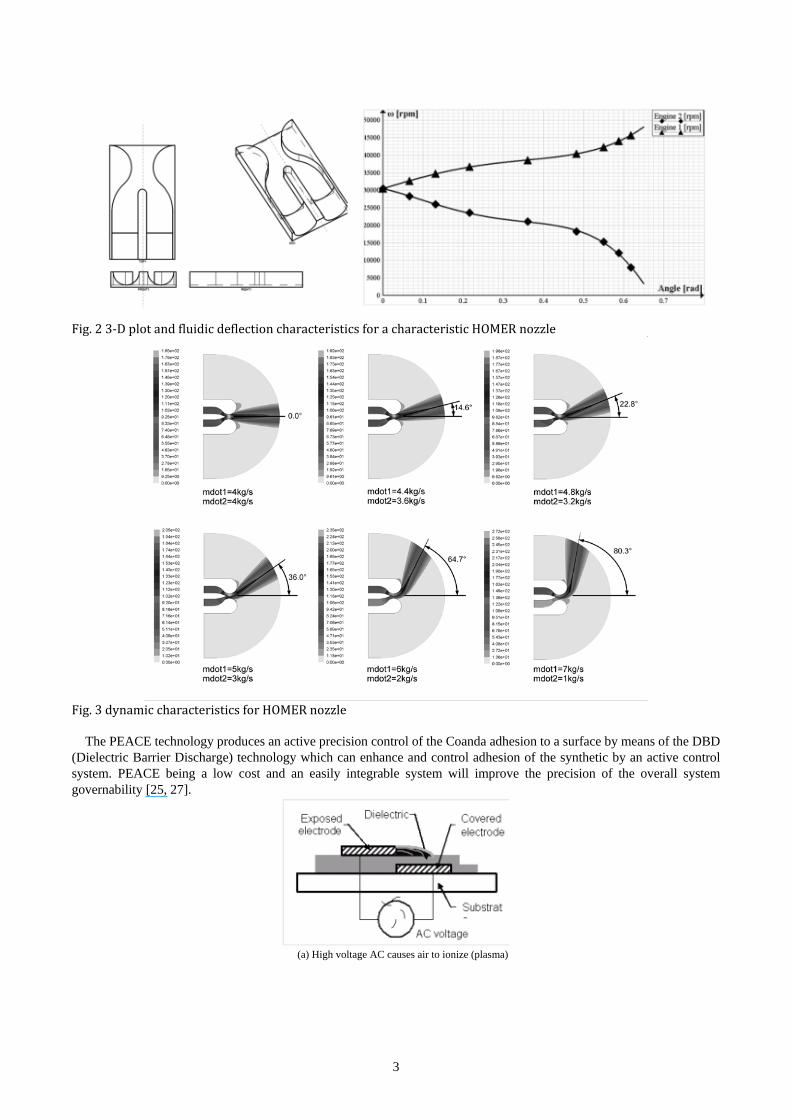
limitations of the preceding Coanda effect nozzles. Based on the initial CFD simulation, the results are very encouraging. In particular it has been verified that it can be easily controlled both in terms of the primitive jet speed or mass flow, presenting excellent performance in both static and dynamic conditions and has a very low inertia (Fig. 1) [10-11, 25]. Similar tests have also been conducted to determine the possibility of control in terms of the rotation speed of two electric turbofans (Fig. 2) also obtaining encouraging results [26]. The HOMER design overcomes the traditional limitations of common Coanda effect Nozzles with an active enhancement and control of adhesion by control jet, which is called PEACE.

2

2'

3

3' 4

5

4

6'

6

7

8

1

Fig. 1 HOMER nozzle design(1-duct, 2,2’-jets, 3,3’-channels, 4-convegence zone, 5-outflow mouth, 6,6’-convex Coanda surfaces, 7-synthtic jet, 8- central septum)

3

Fig. 2 3-D plot and fluidic deflection characteristics for a characteristic HOMER nozzle

Fig. 3 dynamic characteristics for HOMER nozzle

The PEACE technology produces an active precision control of the Coanda adhesion to a surface by means of the DBD

(Dielectric Barrier Discharge) technology which can enhance and control adhesion of the synthetic by an active control system. PEACE being a low cost and an easily integrable system will improve the precision of the overall system governability [25, 27].

(a) High voltage AC causes air to ionize (plasma)

4

(b) Plasma Dielectric Barrier Discharges

(c) Induced air flow with charged particles

Fig. 4 DBD enhancement for HOMER nozzle The integration of HOMER nozzle with the PEACE concept can lead to disruptive potential propulsive system

application shaping novel aerial vehicle architectures and opening up new possibilities based on easy to control and effective use of the Coanda effect.

3. MODELING FOR FIXED-WING TV UAV AND PROPULSION WITH ACHEON NOZZLE 3.1 Thrust-vectoring UAV model

The mathematical model of the fixed-wing UAV with TV is derived from a real fixed-wing UAV the Aerosonde (Fig.5). This UAV model has been selected as it has been benchmarked for many applications. For our proposed fixed-wing UAV with TV, the engine is replaced by a ducted-fan engine configured with the ACHEON thrust-vectoring nozzle.

Fig.5 a benchmark UAV-Aerosonde

The new aircraft model with thrust vector can be presented with a 12-state equation of dynamics and motion. The complete system of equations can be represented as follows:

( , )x f x u= (1)

Where, x is the vector of state variables, and u is the vector of control inputs, which consist of the following elements individually.

[ ]x x y z V p q rγ χ µ α β= (2)

[ ]e a r Ty Tzu Tδ δ δ δ δ= (3)

The notations about the variables above and other variables are introduced in the appendix, and the physical meanings can be seen in Fig. 6. Because the states x , y , z and χ , are assumed to have no effect on the equations governing the other eight states, the 8-vectors of the coupled states are defined as:

[ ]Tx V p q rγ α β µ= (4)

The difference from traditional fixed-wing aircraft is that the two more control inputs are added because of the TV

5

propulsion’s effect. Also, the aircraft dynamics has corresponding revision, which is presented as (5)(6)(7)(8).

Fig. 6 definitions of (angular) velocity components p , q , and r , angle of attack α , sideslip angle β , and external forces F T+ & moments , ,l m n

2 2

2

2

2 2

2 2

2

2

( ) ( )

( ) ( )

( ) ( )

xz x y z y z xz z

x z xz

z xz

x z xz

xz z x

y

x x y xz xz y z x

x z xz

x xz

x z xz

I I I I pq I I I I qrp

I I II l I nI I I

m I r p I I prq

I

I I I I pq I I I I qrr

I I II n I lI I I

− + + − −=

−+

+−

+ − + −=

− + + − −=

−+

+−

(5)

1 [ cos cos ]cos

1tan [ cos sin ] [ sin cos ]cos

1sin cos [ cos sin

1 1 1[( ) cos ] sin cos sin sin

sec [ cos sin ] cos cos tan [tan sin tan ]

(

x z

y x z

q L MgMV

p r T TMV

p r MgMV

Y T T TMV MV MV

g Lp rV MV

Y T

α γ µβ

β α α α αβ

β α α γ µ

β β α β α

µ β α α γ µ β γ µ β

= + − +

− + + − +

= − +

+ + − −

= + − + +

++

) sin costan cos cos [tan sin tan ]

cos sintan cos sin

y x z

x z

T TMV MV

T TMV

α αγ µ β γ µ β

α αγ µ β

−+ +

+−

(6) 1 [ sin cos ]

1 [ sin sin sin ]cos

1 [ sin cos cos cos ]

V D Mg TM

L TMV

T L MgMV

γ α

χ µ µ αγ

γ α µ µ γ

= − − +

= +

= + −

6

(7) cos coscos sinsin

x Vy Vz V

γ χγ χγ

===

(8)

The nonlinear model used here is derived from an original high-fidelity model from the benchmark UAV Aerosonde in Aerosim toolkit[28] , this model is popularly used in aircraft controller design and researches, but some terms such as small aerodynamics force and moment are omitted because of their weak effects on the whole system.

3.2 ACHEON propulsion modeling

With the considerations above it can be verified that the vectoring performance, in terms of vector angle, can be described as a function of the momentum flux ratio for various mass flow inlet values, but also in terms of angular velocity of turbofans.

Base on the description about the principle of ACHEON jet nozzle, a mathematical model can be used to denote the function of the propulsion, which is defined as below.

2 211 11 12 12

2 211 11 11 12 12 12

2 21 1 2 21 21 22 22

2 22 1 2 21 21 21 22 22 22

2 231 31 32 32

2 231 31 31 32 32 32

2 2( , )

*( , ) 2 2

2 2

n n

n n n n

n nTy

n n n nTz

n n

n n n n

k ks s s s

TH k k

FH s s s s

k ks s s s

ω ωε ω ω ε ω ω

ω ω ω ωδ

ω ω ε ω ω ε ω ωδ

ω ωε ω ω ε ω ω

+ + + + = = + + + +

+ + + +

1 1 2

2 1 2

( , )*

( , )HH

ω ωω ω

(9)

Where 1 2( , )ω ω denotes the double fan rotation speeds respectively, 1 1 2( , )H ω ω and 2 1 2( , )H ω ω denotes the mass flow

rates in two channels produced by the double fans. The unknown parameters ( 1, 2,3, 1,2)ijk i j= = and

( 1, 2,3, 1, 2)nij i jω = = in (9) can be obtained by some system identification method based on the data from CFD

simulation result in Fig 2-3. For the sake of simplify for the dynamics, the function matrix F can be rewritten as (10).

11 12

21 22

31 32

k kF k k

k k

=

(10)

The dynamic process from the command signal c Tyc TzcT δ δ to the output variable [ ]1 2ω ω can be described as

below: 11

22

( , , )( , , )

c Tyc Tzc

c Tyc Tzc

P TP T

ω

ω

δ δωδ δω

=

(11)

Where 1Pω and 2Pω denote the functions of cT , Tycδ and Tzcδ . As can be seen from Fig. 2 and Fig. 3, the dynamic response time is very short and about 0.2s because of the merits of no-moving elements for fluidic thrust-vectoring [11-12]and therefore the feedback error is relatively small compared with the response time of the fastest loop (about 2s). Also, The ACHEON propulsion has involved a dedicated close-loop controller inside which is so-called PEACE controller to guarantee its fast response and stability. The details about the PEACE control can be seen in the research work [10-12]. More importantly, no matter what the response time is, the stability of high attack angle maneuvers here is actually guaranteed by two key mechanisms: The first one is the time-scale separation principle, which means that the stability is feasible when the response time of outer slow-loop controller is 4 more times than the one of the inner fast-loop controllers. In our case, the ratio 2 sec/ 0.2 sec=10 is more than 4, so it is feasible from the view of the time-scale separation principle. The second one is a guarantee of fast response and accurate control by the inside PEACE controller for ACHEON, which makes that less error take effects on outside control loop and the feasibility of high-attack angle is strengthen. So, it is feasible to model the ACHEON propulsion as a simple linear model, which can be denoted as below:

c

Tyc Ty

Tzc Tz

T Tδ δδ δ

≈

(12)

And based on the transient CFD simulation result in [12], a boundary restrict conditions for the three TV parameters can be defined as:

7

[ )[ ][ ]

max0,

0, / 2

0, / 2Ty

Tz

T T

δ π

δ π

∈

∈

∈

(13)

Where maxT depends on the throttle command position and engine performance parameters such as thrust-weight ratio, it is variable automatically for surface control with TV. According to the geometric principle of thrust-vectoring force, the 3-dimension thrust force vector can be denoted as below:

cos cossin

cos sin

x Ty Tz

y Ty

z Ty Tz

TT TT

δ δδ

δ δ

= −

(14)

4. INTEGRATED FLIGHT/VECTORED THRSUT CONTROL For UAV applications, the control scheme is important to implement completely self-positioned flight. Especially for jet UAV with TV, the control scheme should not only control some basic flight states such as the attitude states and position states, but also coordinate the surface control and the TV control in an optimized manner.

The overall integrated controller structure of fixed-wing UAV with TV is shown in Fig. 7. It consists of four control loops and one controller allocation in the inner loop. Firstly, The fast loop controller controls the fast dynamic states p , q ,

r and allocates the control inputs aδ , eδ , rδ , Tyδ , Tzδ in the inner loop. Secondly, the angular rates p , q , r are

controlled by the slow states β ,α , µ in the outer loop. Thirdly, the slow states β ,α , µ in wind frame are controlled

by slower states V ,γ , χ , where the thrust force T can be calculated by the velocity V . Finally, the position [y, z] in earth-fixed frame can control the angles γ (flight climbing angle), χ (flight path angle) by the navigation loop controller.

The control allocation module is in charge of allocating control command into two different types of actuators including the surface controls and TV control. Because the NDI control is able to implement separate controls for the 6-dof of the aircraft, especially transform the nonlinear control into linear control, so it is applicable and developed for fixed-wing UAV with TV controller design.

The NDI is applied to the aircrafts equations of motion and are separated into fast dynamic states and slow dynamic states. This is necessary because the airplane has fewer control effectors than the states/outputs to be controlled. In this paper, all the 12 flight states are divided into 4 groups depending on the states requiring speed, and the consequently the four corresponding NDI control loops are designed. Of particular note is that the time scale separation for different loops should be applied in NDI control when controlling different sets of parameters. This means the slower and the faster dynamics are split up. The faster dynamics can then be seen as the inner loop, while the slower dynamics make up the outer loop. For every loop, dynamic inversion is applied separately.

6 DO

F Nonlinear aircraft

Control allocation

Fast dynamics (inner loop)

Fast loop controller

Slow dynam

ics (outer loop)

Slow

er loop controller

slower dynam

ics (outerer loop)

Slower loop controller

Navigation dynam

ics (outerest loop)

Navigation loop controller

+

+

+

+

+

+

+

+

++

+

Thrust Vector control+

VyzγχV

βαµpqr

aδ

eδrδ

TyδTzδ

dp

dq

dr

cp

cq

cr

pq r

dβ

dα

dµ

-

-

-

-

-

--

-

-

-

cβ

cα

cµ

dV

dγ

dχ

cV

cγ

cχ

βαµγχV

dy

dz

yz

cy

cz-

-

cT

Fig. 7 Integrated Controller Structure of fixed-wing UAV with TV

8

When applying the time scale separation, an assumption is made. As input, the inner loop receives a reference value. (For example the desired pitch rate.) The outer loop assumes that this desired value is actually achieved by the inner loop. This is often a valid assumption to make, because the inner loop is much faster than the outer loop. The outer loop (the pitch angle control) then operates by simply supplying the right reference input (the desired pitch rate) to the inner loop [20] .

4.1 Fast loop control (inner loop)

The inner loop shown in Fig. 7 is used to decouple p , q , r and specify the desired, closed-loop, dynamics for the fast controller loop.

( )( )( )

d p c

d q c

d r c

p p pq q qr r r

ωωω

= −= −= −

(15)

The terms, cp , cq and cr , are commands generated by the slow-state control law, to produce the desired rates, dα , dβ and

dµ . The bandwidths pω , qω and rω are each set at 10 rad s-1, which is about as high as they can be without risk of exciting structural modes and being subject to the bandwidth limitations of the control actuators. Equation (5) can be written in the form of equation (16) based on the affine form of the aerodynamic moment data.

( ) ( )f f

pq F x G x ur

= +

(16)

Here, x is the 8-vector representation of the aircraft states, defined in equation(4), while u is the 5-vecto r representation of the control surface deflections, defined below.

a

c

r

Ty

Tz

u

δδδδδ

=

(17)

( )fF x is a 3-vector function, defined by equation (18), and ( )fG x is a 3*5 matrix function, defined by equation (25),

which links the control deflections to the angular accelerations. The subscript f refers to the fast-state equations.

( )( ) ( )

( )

p

f q

r

f xF x f x

f x

=

(18)

Where the elements of ( )fF x are given by

2

2 2

2

ˆˆ( )

( ) ( )

z xzp

x z xz

xz x y z y z xz z

x z xz

I L I Nf x

I I I

I I I I pq I I I I qrI I I

+=

−

− + + − −+

−

(19)

2 2ˆ ( ) ( )( ) xz z x

qy

M I r p I I prf x

I+ − + −

= (20)

2

2 2

2

ˆˆ( )

( ) ( )

x xzr

x z xz

x x y xz xz y z x

x z xz

I N I Lf x

I I I

I I I I pq I I I I qrI I I

+=

−

− + + − −+

−

(21)

Here, L̂ , M̂ and N̂ are respectively the aerodynamic rolling, pitching and yawing moments, produced with the control surface deflections set to zero. The momentsL , M and N are derived from the overall momentsL , M ,N , and it mainly depend on the geometry of the aircraft and current states. The relationship can be denoted as below.

9

21 .2

l

A m

n

L bCM V S c CN b C

ρ = ⋅

(22)

[ ][ ][ ]

ˆ

ˆ

ˆ

sl l l l lr lp l a a l r r

sm m m m mq m e e

sn n n n nr np na a n r r

C C C C C r C p C C

C C C C C q C

C C C C C r C p C C

β δ δ

α δ

β δ

β δ δ

α δ

β δ δ

= + = + + + + = + = + +

= + == + + + +

(23)

2

ˆˆ1 ˆˆ .2ˆˆ

l

A m

n

bCL

M V S c C

N b C

ρ

=

⋅

(24)

Where ˆiC and s

iC are aerodynamic coefficients. From (22)-(24) we can see that, the whole moments include two parts: the

former one ˆiC depends on the geometry of the aircraft and current states; the last one s

iC depends on the surface control deflection angles. For the usual controller configurations, ( )fG x has the form:

( )

( ) 0 ( ) ( ) 0

0 ( ) 0 0 ( )

( ) 0 ( ) ( ) 0

a r Ty

c z

a r Ty

f

p p p

q q

r r r

G x

g x g x g x

g x g x

g x g x g x

δ δ δ

δ δ

δ δ δ

=

(25) The non-zero elements of ( )fG x are given by the following expressions:

2

( ) ( )( ) a a

a

z l xz np

x z xz

I C I Cg x qSb

I I Iδ δ

δ

α α+=

− (26)

2

( ) ( )( ) r r

r

z l xz np

x z xz

I C I Cg x qSb

I I Iδ δ

δ

α α+=

− (27)

2( )180Ty

xz Tp

x z xz

I Txg xI I Iδ

π−=

− (28)

( )( ) e

e

mq

yy

qScCg x

Iδ

δ

α= (29)

( )180Tz

Tq

yy

Txg xIδ

π= (30)

2

( ) ( )( ) a a

a

x n xz lr

x z xz

I C I Cg x qSb

I I Iδ δ

δ

α α+=

− (31)

2

( ) ( )( ) r r

r

x n xz lr

x z xz

I C I Cg x qSb

I I Iδ δ

δ

α α+=

− (32)

2( )180y

x Tr

x z xz

I Txg x

I I Iδπ−

=−

(33)

The terms, ( )Typg xδ , ( )

Tzqg xδ and ( )Tyrg xδ are derived from the following expressions for the pitching and yawing

moments produced by TVC: sin( )

cos( )sin( )T T z T Tz

T T y T Tz Ty

M x T x TN x T x T

δδ δ

= == − = −

(34)

Here Tx is the distance from the engine nozzle to the center of mass. The three formulations of (28), (30) and (33) are derived as below:

10

A. Derivation of (28) The (28) is derived from the rolling equations as below.

2 2

2 2

( ) ( )xz x y z y z xz z z xz

x z xz x z xz

I I I I pq I I I I qr I L I Np

I I I I I I− + + − − +

= +− −

(35)

From (35) we can see, the term with relationship yaw moment N is 2xz

x z xz

I NI I I−

, where it can be split two parts because of

one yaw moment N is from surface aerodynamics (with all surface flips control set to be zero) and the other one TN is from thrust vector control, it is denoted as below.

2 2 2xz xz xz T

x z xz x z xz x z xz

I N I N I NI I I I I I I I I

= +− − −

(36)

According to the second formulation of (34), we can get its simplification as below.

T T y T TyN x T x Tδ= − = − (37)

So, the last term of (36) can be denoted as below.

' '2 2 2

( )180 Ty

xz T Tyxz T xz TTy Ty

x z xz x z xz x z xzp

I x TI N I x TI I I I I I I I

gI δ

δ π δ δ−

= = − =− − −

(38)

Where 'Tyδ is in the unit of degree, so we can get (28) as:

2( )180Ty

xz Tp

x z xz

I Txg xI I Iδ

π−=

− (39)

B. Derivation of (30)

The (30) is derived from the rolling equations as below. 2 2( ) ( )xz z x

y

M I r p I I prq

I+ − + −

= (40)

From (40) we can see, the term with relationship pitching moment M is y

MI

, where it can be split two parts because of

one moment M is from surface aerodynamics (with all surface flips control set to be zero) and the other one TM is from thrust vector control, it is denoted as (41).

T

y y y

MM MI I I

= + (41)

According to the formulation sin( )T T z T TzM x T x T δ= = , we can get its simplification as (42):

T T z T TzM x T x Tδ= = (42)

So, the last term of (41) can be denoted as (43).

' '

180 Tz

T T Tz TTz Tz

y y yqgM x T x T

I I I δδ π δ δ= = = (43)

Where 'Tzδ is in the unit of degree, so we can get the (30) as below.

( )180Tz

Tq

yy

Txg xIδ

π= (44)

C. Derivation of (33) The derivation of (33) is similar with (28) and has the similar formulation. Both of them involve the TN and Tyδ . So, one gets:

2( )180y

x Tr

x z xz

I Txg x

I I Iδπ−

=−

(45)

That ends of the derivations. Having defined the terms, ( )fF x and ( )fG x above, the control inputs can be derived from equation (16) based on the NDI principle.

11

1

( )( ) ( )

( )

a

d pc

f d qr

d rTy

Tz

p f xu G x q f x

r f x

δδδδδ

−

= = −

(46)

For the purpose of minimizing the likelihood of saturation the normalized input vector, u , was defined by dividing each of the control deflections by its maximum displacement limit as follows:

max

max1

max max

max

max

ˆˆa a

e e

r r

Ty Ty

Tz Tz

u u

δ δ

δ δδ δδ δδ δ

−

= ∆ =

(47)

Where max∆ is a diagonal, 5*5 matrix with elements defined as:

{ }max max max max max maxˆ, , , ,a e r Ty Tzdiag δ δ δ δ δ∆ = (48)

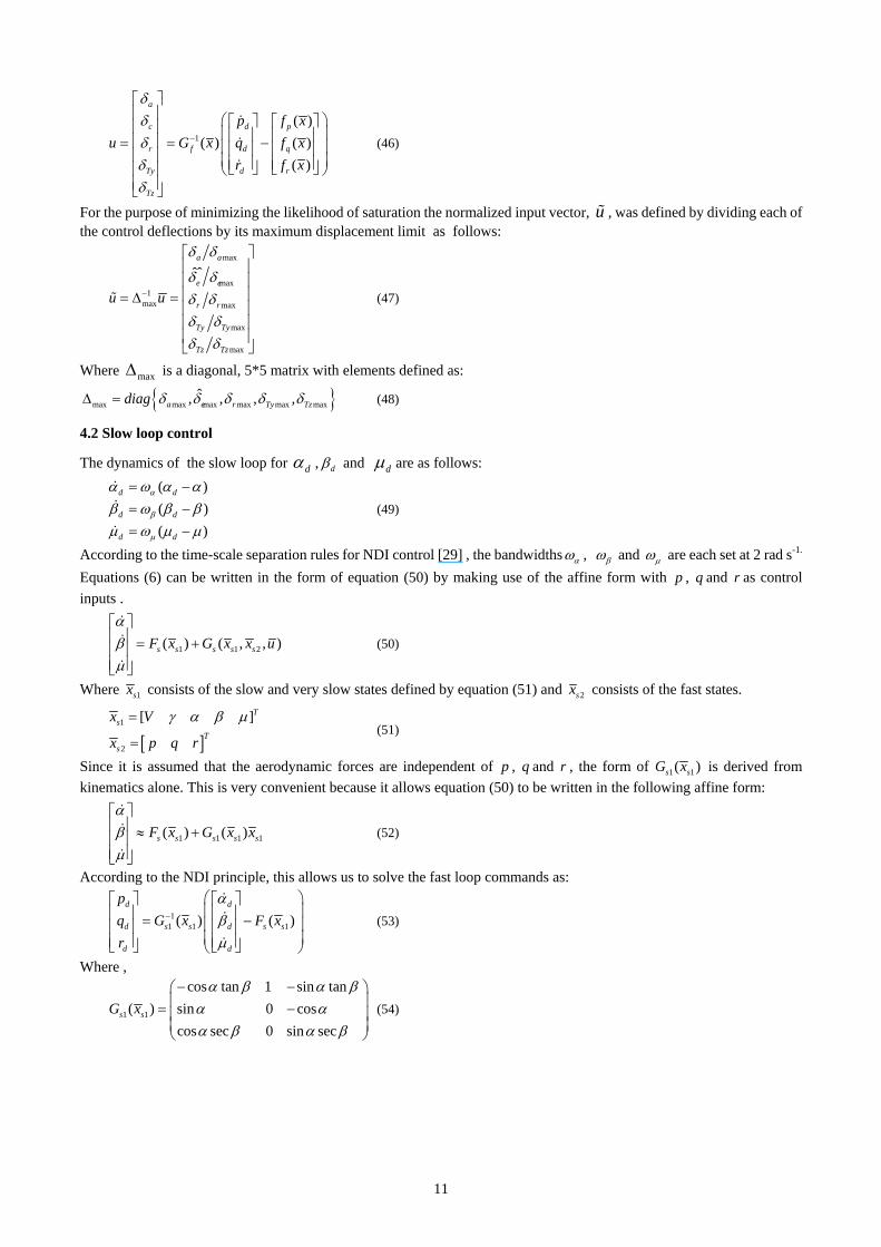
4.2 Slow loop control

The dynamics of the slow loop for dα , dβ and dµ are as follows: ( )( )( )

d d

d d

d d

α

β

µ

α ω α αβ ω β βµ ω µ µ

= −= −= −

(49)

According to the time-scale separation rules for NDI control [29] , the bandwidths αω , βω and µω are each set at 2 rad s-1. Equations (6) can be written in the form of equation (50) by making use of the affine form with p , q and r as control inputs .

1 1 2( ) ( , , )s s s s sF x G x x uαβµ

= +

(50)

Where 1sx consists of the slow and very slow states defined by equation (51) and 2sx consists of the fast states.

[ ]1

2

[ ]Ts

Ts

x V

x p q r

γ α β µ=

= (51)

Since it is assumed that the aerodynamic forces are independent of p , q and r , the form of 1 1( )s sG x is derived from kinematics alone. This is very convenient because it allows equation (50) to be written in the following affine form:

1 1 1 1( ) ( )s s s s sF x G x xαβµ

≈ +

(52)

According to the NDI principle, this allows us to solve the fast loop commands as:

11 1 1( ) ( )

d d

d s s d s s

d d

pq G x F xr

αβµ

−

= −

(53)

Where ,

1 1

cos tan 1 sin tan( ) sin 0 cos

cos sec 0 sin secs sG x

α β α βα αα β α β

− − = −

(54)

12

1

1 1 1

1

1 [ cos cos sin ]cos( )

1( ) ( ) [ cos sin cos sin cos ]( )

[tan sin tan ]

1 [ tan cos cos cos cos tan ]

[tan (sin sin cos sin cos ) tan sin ]

x

s

s s s x

s

x

L Mg TMVf x

F x f x Mg Y TMV

f x LMV

Y MgMV

TMV

α

β

µ

γ µ αβ

γ µ β β α

γ µ β

γ µ β γ µ β

γ µ α µ β α β α

− + − = = + + −

+

+ −

− +

(55)

Comments: from the derivation process about ( )fF x and 1 1( )s sG x above we can see, the model used in NDI controller design here is a simplified nonlinear model and very different from the original system model. Although it will cause control errors, this simplification is valuable for more convenient engineering implementation because some weak terms which affects system nonlinearity and dynamics are omitted. Also, it can still keep that the control error is acceptable.

4.3 Very-slow loop control

The dynamics of the slower loop for dV , dχ and dγ are as follows: ( )( )( )

d V d

d d

d d

V V V

χ

γ

ωχ ω χ χγ ω γ γ

= −= −= −

(56)

According to the time-scale separation rules for NDI control [29], the bandwidths Vω , χω and γω are each set at 0.2 rads-1.

Equations (7) can be written in the form of equation (56) by making use of the affine form with dα , dβ and dµ as control inputs.

1 [ sin cos ]

1 [ sin sin sin ]cos

1 [ sin cos cos cos ]

d

d

d

V D Mg TM

L TMV

T L MgMV

γ α

χ µ µ αγ

γ α µ µ γ

= − − +

= +

= + −

(57)

Provided that both V and cosγ are non-zero, equations (57) can be rearranged to give the required velocity bank angle,

cµ , in terms of dχ and dγ .

cos( )arctan

cos( )d

cd

VV g

χ γµ

γ γ

= +

(58)

The engine thrust command, cT , and cα can be determined from equations (59), which are derived from equations(7). However, the lift, L , and drag, D , are nonlinear functions of V and α , so an iterative procedure is used to compute the values of cT and cα satisfying equations (60). Since V , χ and γ change much more slowly than α , their current values are used in the iteration algorithm.

( )1 ( , ) sin( )cosc d c

c

T MV D V Mgα γα

= + + (59)

sin ( , )cos sin cos cos cos

c c c

c d c d c

T L VMV MV Mg

α αγ µ χ µ γ γ µ+ =

+ +

(60)

4.4 Position control

As a result of the inherent metrics of fixed-wing aircraft, the positions y and z are controllable while the position x is not directly controlled in earth frame and controlled indirectly by forward velocity. Comparing fixed-wing aircrafts with rotor aircrafts such as helicopters, because the forward velocity is very fast, the x position generally is difficult to control

13

while the velocity is controllable. In some practical applications such as missiles attacking, generally y, z positions and the velocity of forward velocity V is used as the control variables but not x, y, z position .The rough x position in earth frame is controllable by controlling the velocity. So, here only y and z positions are considered in our cases. The dynamics of the position control loop for y-axis position dy and z-axis position dz are as follows:

( ) cos sin( ) sin

d y d c c c

d z d c c

y y y Vz z z V

ω γ χω γ

= − == − =

(61)

Based on equations(61), cV , cγ and cχ can be solved as

arcsin dc

c

zV

γ

=

(62)

2 2arcsin d

c

c d

y

V zχ

= −

(63)

00

d cy

d cz

y y yz z z

ωω

− = −

(64)

The bandwidths yω and zω are each set at 0.02 rad s-1

5. FLIGHT TEST AND VALIDATION RESULTS In order to show the performance and efficiency of the integrated flight/thrust vectoring control scheme, the proposed control scheme is validated for different flight conditions and scenarios. Two sets of flight scenarios, which include cascaded control and maneuver control, are executed to test performance of the jet aircraft with TV in different applications.

The key parameters of the UAV model and some initial conditions are listed as below: Mass weight of the aircraft:

13.5M kg= Span length:

2.8956b m= Dynamic pressure area:

20.55S m= Distance between nozzle and central gravity point: 1.56Tx m= , the initial condition parameters are listed as:

[ ] [ ][ ]

0

0

0

0

27 /[ ] [0 0 0]

0 0 0

[ ] 0 0 1000

V m s

p q r

x y z

ϕ θ ψ=

=

=

=

The aerodynamic coefficients can be seen in the configuration file of Aerosonde UAV in Aerosim blockset. The moments of inertia:

2

2

2

2

2

2

0.8244

1.135

1.759

0.1

0

2

0

04

x

y

z

xy

xz

yz

I kg m

I kg m

I kg m

J kg m

J kg m

J kg m

= = =

= =

=

The maximum thrust force of the propulsion system:

max 20T N=

5.1 Cascaded Control performance

As described in Fig. 7 , the overall control scheme with the four loops cascaded structure aims to control all the flight states into the four groups because the states converge at different speeds. In order to validate the availability of the four control loops, the four control loops are tested from inner to outer respectively based on corresponding control input commands.

14

1) Fast loop control

The fast loop controller aims to control the angular rates, which is the fastest state that has the closest relationship with the surface control and TV control. Because the rotation moment torques have direct effect on the angular rates, the surface control and TV control change the deflection angles to implement variations of the control torques. The tracking results for the command angular rate control signals are depicted in Fig. 8, showing that the actual angular rates can converge into the commanded angular rates very quickly (less than 3 seconds) under the common actions of both surface control and TV control.

Fig. 8 fast loop controller tracking result

The actions of surface controls and TV controls can be reflected as flap angle deflection and TV angle deflection variations as shown in Fig. 9. For the pitch control, the Z-axis deflection angle has some trends with elevator deflection angle and both deflection angles are small enough to make the systemic control energy minimal, which demonstrates that the surface control and TV control bear the control action well under coordination from the optimized NDI control law. For the yaw control, The Y-axis deflection angle has some trends with rudder deflection angle, which also means that it follows the cooperation rules under coordination from the optimized NDI control law.

0 2 4 6 8 10-15

-10

-5

0

5

10

15

t(s)

Def

lect

ion

angl

es fo

r fla

psan

d ve

ctor

ing

thru

st(d

egre

e/s)

Rudder deflectionY-axis deflectionZ-axis deflectionElevator deflectionAileron deflection

Fig. 9 deflection angular variation for surface controls and TVC

15

2) Slow loop control

The slow loop controller aims to control the attitude parameters in the wind reference frame, which are the slow states and have the closest relationship with the attitude angle rates in body reference frame. The aerodynamics forces are the functions of the attitude angle in the wind reference frame，so it is important to control the aerodynamics forces by adjusting its attack angle and side-sliding angle. As a result of the approximation and omitting principle of the NDI control law, the aerodynamic forces derived from variations of attitude angles in the wind reference frame make the main contributions to the control of aerodynamics forces when compared to the flap deflection angle variations. Therefore, there are some acceptable errors for the attitude tracking but it is more suitable for an engineering implementation.

0 10 20 30 40 50

0

2

4

6

8

10

12

t(s)

attit

ude

angl

e(de

gree

)

command attack anglecommand side-sliding anglecommand velocity roll angleActual attack angleActual side-sliding angleActual velocity roll angle

Fig. 10 slow loop controller tracking result

The tracking results for command attack angle and side-sliding angle control as well as velocity roll angle are shown in Fig. 10. Although there are some tracking errors (less than one degree) for three slow states, the errors converge to zero gradually and it is acceptable for practical engineering implementation.

In order to demonstrate the control effectiveness in different high-attack angles, attack angles with 10 degree, 30 degree and 50 degree are selected as command input attack angles. The control trajectories of the three high-attack-angle scenarios are shown in Fig. 11.

Fig. 11 Control trajectories subjected to different attack angles

16

From the results we can see that the command attack angles are well tracked in a manner of convergence. Because of the effect from the control law simplifications, there are some fluctuations at the beginning, but it is acceptable and meaningful for engineering application with the merit of simpler nonlinearity calculations.

3) Very-slow loop(navigation loop) control

The very-slow loop controller aims to control the flight velocity, flight climbing angle and flight path angle, which are the very-slow states and have closet relationship with the thrust and attitude angle rates within the wind reference frame. For the sake of convenience, the output side-slipping command angle rate is generally set to zero.

A navigation loop control tracking trajectory is shown in Fig. 12. The command input

is[ ] 30 / 0 10V m sγ χ = , the actual velocityV , flight path angle χ and flight climbing angle γ track

well the command values.

Fig. 12 Very-slow loop controller tracking result

In order to validate the close-loop control effects, a specified command input is defined as below.

30 ( / )0 ( )10* * /180( )

V m srad

t radγχ π

= = =

(65)

This command input indicates that the UAV should fly around a circle with the flight speed 30 ( / )m s and the flight path

angular rate 10* /180( / )rad sπ . And it also means that it should take about 36 seconds to finish a circle trajectory flight. As can be seen from the Fig. 13, the UAV flight follows well with the specified fight path although there are some errors

due to the initial conditions. It takes a little more than 36 seconds to finish the flight task.

17

Fig. 13 very-slow states tracking results

4) Position loop control

The position loop controller aims to control the flight y-axis and z-axis position, which are the slowest states and has direct relationship with flight climbing angle rate and flight path angle rate. Because the x-axis position is generally uncontrollable for jet fixed-wing aircrafts and it has direct relationship with flight velocity, the command velocity is still set to be constant for sake of convenience. Two flight path scenarios are respectively designed to validate the effectiveness of the position control.

Fig. 14 an altitude variation trajectory result

Fig. 14 and Fig. 15 depict an altitude variation trajectory under a square command signal with the duty ratio 50% and

-1000

0

1000

2000

3000

4000

5000

6000-50 0 50

-100

-50

0

50

100

X (m)

18

magnitude 50m, and the controller works without actuator saturation. Fig. 16 depicts the optimized tracking result with controller parameter tuning. As can be seen from Fig. 15, the actual trajectory tracks well with the command trajectory and it takes about 50 seconds to track the command altitude because of the slowest states variation and corresponding controller adjustment. As can be seen from Fig. 16, the tracking convergence speed is well improved by the controller parameters tuning.

Fig. 17 and Fig. 18 depict a y-axis position variation trajectory under a square command signal with the duty ratio 50% and magnitude 50m, and the controller works without actuator saturation. Fig. 19 shows the optimized tracking result with controller parameter tuning. As can be seen from Fig. 18, the actual trajectory also tracks well with the command trajectory. As can be seen from Fig. 19, the tracking convergence speed is well improved by the controller parameters tuning.

Fig. 15 altitude tracking result without actuator saturation

Fig. 16 Altitude tracking result with controller parameter tuning

Fig. 17 a y-axis position variation result

-1000

0

1000

2000

3000

4000

5000

6000-50 0 50 100

-100

10

Y (m)

X (m)

19

Fig. 18 y-z position tracking results without actuator saturation

Fig. 19 y-z position tracking result with controller parameter tuning

Finally, in order to describe the control performance, some statistical characteristics on tracking errors of the four loops

control are given in Tab. 1. As can be seen from this table, all the tracking errors are bounded and acceptable for engineering. Especially for slow-loop control, and the error bound is restricted under 1 degree, which satisfy the requirement of controller design for attack angles.

Tab. 1 Control convergence max error bounds

Fast loop control Slow loop control Very-slow loop

control Position loop control

α β µ χ γ z position y position

Convergence Max error bound 0.00001rad/s 1 ° 0.1° 0.5° 0.1° 0.01° 1m 3 m

5.2 Maneuver flight performance

Flight maneuverability is an important merit of the fixed-wing aircraft with TV and also an important indicator for modern combating aircraft. In order to assess the flight maneuverability performance of the TVC aircraft with our proposed configuration, two types of flight maneuvering scenarios, which include VVR and high-attack-angle, are simulated and the corresponding results are available under the specified control input conditions.

1) Velocity vector roll

The VVR maneuver can implement a 360 quickly rolling action, which generally needs to be addressed by a nonlinear controller to avoid the coupling effects among the 6 DOF. In our flight simulations, the VVR maneuver flight action can be done by setting the roll angular rate to a non-zero constant and the pitch and yaw angular rates to zero.

Fig. 20 depicts the VVR maneuver flight trajectory under a given control input condition: 40* /180( / )0 ( / )0 ( / )

cmd

cmd

cmd

p pi rad sq rad sr rad s

===

(66)

It can be inferred from the defined control input condition that it should take about 9 seconds to finish the VVR because it holds that 360 / 40 9= . Fig. 20 shows that the fixed-wing UAV with TV follows well the required maneuver trajectory.

As can be seen from Fig. 21, all the surface flaps and TV deflections take part in the VVR action. The trends of the elevator deflection angle and the z-axis deflection angles are kept the same and indicate a decent trend for the altitude. The trends of the rudder deflection angle and the y-axis deflection angle are kept the same and indicate a right-oriented trend for

20

the yaw angle. The right-oriented roll action follows well with the variation trend of the aileron deflection angle.

-2000

200400

600800-40 -20 0 20

-80

-60

-40

-20

0

20

Y (m)X (m)

Z (m

)

Fig. 20 VVR flight trajectory

0 5 10 15 20 25-20

-15

-10

-5

0

5

10

15

20

25

30

t(s)

Def

lect

ion

angl

es fo

r fla

psan

d ve

ctor

ing

thru

st(d

egre

e/s)

Aileron deflectionElevator deflectionRudder deflectionZ-axis deflectionY-axis deflection

Fig. 21 surface control and TVC deflection angles subjected to VVR maneuver

2) High attack angle

The high-attack angle maneuver can keep the aircraft in a high-attack angle attitude with a low-speed flight velocity, which is very useful for the close -range combat maneuver performance of jet aircraft. In order to test the maneuverability of our proposed aircraft, a 70-degree attack angle command is set to evaluate the performance.

Fig. 22 depicts the flight trajectory of the fixed-wing jet aircraft with TV under the condition that the command attack

21

angle is set to be 70 degree. It takes about 15 seconds to reset the aircraft attack angle from 0 degree to 70 degree. Although there are fluctuations for the attack angle during the initial stage due to the controller’s adjustment, it begins to approach to be constant after about 15 seconds.

-50

0

50

100

150

200

250 -200

20

-20

0

20

40

Y (m)

X (m)

Z (m

)

Fig. 22 70 degree attack angle flight trajectory result

As can be seen from Fig. 23, both the z-axis TVC deflection and elevator, take part in the formulation of the high-attack angle maneuver action. With the help of Z-axis TVC, the elevator only needs to contribute approximately 20 degree of deflection to finish the 70-degree attack angle maneuver action, which is difficult for traditional fixed-wing aircraft with only surface controls.

0 5 10 15 20 25-80

-60

-40

-20

0

20

40

60

80

100

120

t(s)

Def

lect

ion

angl

es fo

r fla

psan

d ve

ctor

ing

thru

st(d

egre

e/s)

Z-axis deflectionElevator deflectionY-axis deflectionRudder deflectionAileron deflection

Fig. 23 surface control and TVC deflection angles subjected to high attack angle maneuver

22

6. CONCLUSION This paper proposes an integrated flight/thrust vectoring control scheme for fixed-wing UAVs based on the novel ACHOEN propulsion system. The novel large-deflection angle TV nozzle, ACHEON, is adopted and a completely self-positioning control scheme based on the NDI control law for the proposed fixed-wing UAV with TV is developed. The maneuver performance of this new configuration is assessed on a modified Aerosonde UAV model and flight test results demonstrate its improvement in maneuver ability based on TVC. Future work will expand the ACHEON propulsion model to a high- fidelity model based on experiment data and will consider the energy optimization problem of electrically-powered thrust for V/STOL.

References: [1] M. R. Schaefermeyer, "Aerodynamic Thrust Vectoring For Attitude Control Of A Vertically Thrusting Jet Engine,", UTAH STATE UNIVERSITY, 2011. [2] M. Murty, M. S. Rao and D. Chakraborty, "Numerical simulation of nozzle flow field with jet vane thrust vector control," Proceedings of the Institution of Mechanical Engineers, Part G: Journal of Aerospace Engineering, vol.224, pp. 541-548, 2010. [3] D. Kirk, "Experimental and Numerical Investigations of a High Performance Co-Flow Jet Airfoil," Master dissertation, University of Miami, 2009. [4] F. Sagha and A. Banazadeh, "In-Trim Flight Investigations of a Conceptual Fluidic Thrust-Vectored Unmanned Tail-Sitter Aircraft," vol.3, pp. 125-133, 2006. [5] G. Raman, S. Packiarajan, G. Papadopoulos, C. Weissman and S. Raghu, "Jet thrust vectoring using a miniature fluidic oscillator," Aeronautical Journal, vol.109, pp. 129-138, 2005. [6] A. Buonanno, D. Drikakis, C. Papachristou, A. Savvaris, C. Vamvakoulas and C. Warsop, "Computational investigation of the DEMON unmanned air vehicle thrust vectoring system," Proceedings of the Institution of Mechanical Engineers, Part G: Journal of Aerospace Engineering, vol.224, pp. 387-394, 2010. [7] S. B. Lazarus, A. Tsourdos, P. Silson, B. White and R. Żbikowski, "Unmanned aerial vehicle navigation and mapping," Proceedings of the Institution of Mechanical Engineers, Part G: Journal of Aerospace Engineering, vol.222, pp. 531-548, 2008. [8] H. Edge, J. Collins, A. Brown, M. Coatney, B. Roget and N. Slegers, et al., "Lighter-Than-Air and Pressurized Structures Technology for Unmanned Aerial Vehicles (UAVs),", 2010. [9] F. Saghafi and A. Banazadeh, "Investigation on the flight characteristics of a conceptual fluidic thrust-vectored aerial tail-sitter," Proceedings of the Institution of Mechanical Engineers, Part G: Journal of Aerospace Engineering, vol.221, pp. 741-755, 2007. [10] M. Trancossi and A. Dumas, "ACHEON: Aerial Coanda High Efficiency Orienting-jet Nozzle," SAE Technical Paper, pp. 27-37, 2011. [11] M. Trancossi and A. Dumas, "CFD based design of a nozzle able to control angular deflection," in Proc. 2011 ASME 2011 International Mechanical Engineering Congress & Exposition. [12] M. Trancossi and A. Dumas, "Coanda Synthetic Jet Deflection Apparatus and Control," SAE Paper, pp. 18-21, 2011. [13] J. C. Páscoa, A. Dumas, M. Trancossi, P. Stewart and D. Vucinic, "A review of thrust-vectoring in support of a V/STOL non-moving mechanical propulsion system," Central European Journal of Engineering, vol.3, pp. 374-388, 2013. [14] W. Lei and W. Lixin, in The 2nd International Conference on Computer Application and System Modeling, France, 2012, pp. 825-827. [15] P. V. M. Simpl´ıcio, "Helicopter Nonlinear Flight Control using Incremental Nonlinear Dynamic Inversion,", Delft University of Technology, 2011. [16] A. H. Bajodah and I. Hameduddin, "Aircraft maneuvering control using generalized dynamic inversion and semidefinite Lyapunov functions," in Proc. 2010 Control Applications (CCA), 2010 IEEE International Conference on, pp. 1825-1831. [17] A. Ko, O. J. Ohanian and P. Gelhausen, "Ducted fan UAV modeling and simulation in preliminary design," in Proc. 2007 AIAA modeling and simulation technologies conference and exhibit. [18] R. Hindman and W. M. Shell, "Design of a missile autopilot using adaptive nonlinear dynamic inversion," in Proc. 2005 Proceedings of the American Control Conference, pp. 327. [19] M. Harefors and D. G. Bates, "Integrated propulsion-based flight control system design for a civil transport aircraft," in Proc. 2002 Control Applications, 2002. Proceedings of the 2002 International Conference on, pp. 132-137. [20] A. K. Vinayagam and N. K. Sinha, "An assessment of thrust vector concepts for twin-engine airplane," Proceedings of the Institution of Mechanical Engineers, Part G: Journal of Aerospace Engineering, 2013. [21] X. Yang, "Research on Control Technology of the Unmanned Aerial Vehicle Based on TVC," Master dissertation, Nanjing University of Aeronautics and Astronautics, 2012. [22] C. Yuhua, "Flight Control of the Unmanned Aerial Vehicle Based on TVC," Master dissertation, Nanjing University of Aeronautics and Astronautics, 2009. [23] Q. Wang and R. F. Stengel, "Robust nonlinear flight control of a high-performance aircraft," Control Systems Technology, IEEE Transactions on, vol.13, pp. 15-26, 2005. [24] P. M. Lodge and C. Fielding, "Thrust Vector Control and Visualisation for STOVL Aircraft," in Proc. 2000 RTO Symposium on Active Control Technology. [25] M. Subhash and A. Dumas, "Computational Study of Coanda Adhesion Over Curved Surface," SAE International Journal of Aerospace, vol.6, pp. 260-272, 2013. [26] M. Trancossi, in IMECE 2013 – ASME International Mechanical Engineering Congress and Exposition, San Diego, CA, USA , 2013, pp. 63459. [27] M. Subhash, M. Trancossi and A. Dumas, in International CAE Conference 2013, Verona, Italy, 2013. [28] U. D. Version, , http://www. u-dynamics. com. [29] S. A. Snell, D. F. NNS and W. L. ARRARD, "Nonlinear inversion flight control for a supermaneuverable aircraft," Journal of

23

Guidance, Control, and Dynamics, vol.15, pp. 976-984, 1992.

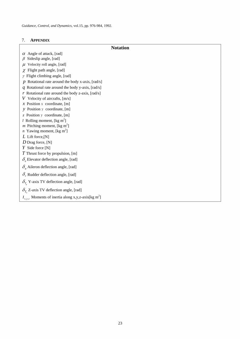
7. APPENDIX

Notation α Angle of attack, [rad] β Sideslip angle, [rad] µ Velocity roll angle, [rad] χ Flight path angle, [rad] γ Flight climbing angle, [rad] p Rotational rate around the body x-axis, [rad/s] q Rotational rate around the body y-axis, [rad/s] r Rotational rate around the body z-axis, [rad/s] V Velocity of aircrafts, [m/s] x Position x coordinate, [m] y Position y coordinate, [m] z Position y coordinate, [m] l Rolling moment, [kg m2] m Pitching moment, [kg m2] n Yawing moment, [kg m2] L Lift force,[N] D Drag force, [N] Y Side force [N] T Thrust force by propulsion, [m]

eδ Elevator deflection angle, [rad]

aδ Aileron deflection angle, [rad]

rδ Rudder deflection angle, [rad]

δyT Y-axis TV deflection angle, [rad]

zTδ Z-axis TV deflection angle, [rad]

, ,x y zI Moments of inertia along x,y,z-axis[kg m2]