
Integrable Models in Physics - International Institute … · Integrable Models in Physics ... •...
87
Integrable Models in Physics Angela Foerster Universidade Federal do Rio Grande do Sul Instituto de Física, Porto Alegre talk presented at "Quantum non-equilibrium phenomena" June, Natal, 2016 Integrable Models in Physics – p. 1/87
Transcript of Integrable Models in Physics - International Institute … · Integrable Models in Physics ... •...
Integrable Models in PhysicsAngela Foerster
Universidade Federal do Rio Grande do Sul
Instituto de Física, Porto Alegre
talk presented at "Quantum non-equilibrium phenomena"
June, Natal, 2016
Integrable Models in Physics – p. 1/87
Integrable Models:Quantum models which can be exactly solved by Bethe Ansatz
IM can be found in different areas, such as:
• Statistical Physics
• Quantum Field Theory
• ***Condensed Matter
• ***Ultracold Atoms
Present some integrable models in CM and UA,
focusing on some prominent examples
Integrable Models in Physics – p. 2/87
OUTLINE
1- Introduction
2- Integrable models in Condensed Matter• Spin ladder model
3- Integrable models in Ultracold Matter
• Bosonic quantum tunneling models
• Fermi gas with polarization
• Few particles system
4- Breaking the integrability
5- Conclusions
Main emphasis: results and physical propertiesIntegrable Models in Physics – p. 3/87

1 - INTRODUCTION
Integrable Models in Physics – p. 4/87
Importance of the study of integrable models:
• They serve as a test for computer analysis and analytic
methods for realistic systems, where only numerical
calculations and perturbative methods may be applied;
• They serve as a laboratory for investigations for the
situations (1) where the mean field treatment fails (quantum
fluctuations are large) or (2) which cannot be described via
perturbation theory (strong coupling);
• From the mathematical point of view, they provide explicit
realization of algebraic structures, such as Lie algebras and
quantum groups;
Integrable Models in Physics – p. 5/87
Importance of the study of integrable models:
• From the experimental point of view, there are materials
which behave like (quasi) 1D systems, such as KCuF3,
Sr2CuO3, (C5D12N)2CuBr4, (5IAP2CuBr42H2O),
Cu2(C5H12N2)2Cl4, ...... which can be well described by
integrable spin chains and ladders;
• Some integrable systems have been realized in the lab in
the context of ultracold atoms.
Integrable Models in Physics – p. 6/87

2 - Integrable models in CondensedMatter
Integrable Models in Physics – p. 7/87
Spin ladder systems
Importance:Some compounds have been realized experimentallywith a ladder structure:
SrCu2O3
La1−xSrxCuO2, 5
Sr14−xCaxCu24O41
Cu2(C5H12N2)Cl4
CaV2O5
KCuCl3
Integrable Models in Physics – p. 8/87
• Different experiments using these compounds doreport on the existence of a spin gap in the energyspectrum: magnetic susceptibility, NMR techniq.
• In some of these even leg-ladder compoundssuperconductivity has been detected upon holedoping (chemical substitution)detected in resistivity curves
• It has been observed that:Even leg ladders exhibit a gap;Odd leg ladders do not exhibit a gap.
Integrable Models in Physics – p. 9/87
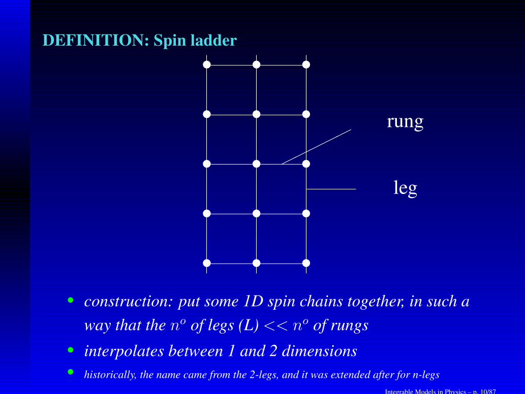
DEFINITION: Spin ladder
• • •
• • •
• • •
• • •
• • •
✟✟
✟✟✟
rung
leg
• construction: put some 1D spin chains together, in such a
way that the no of legs (L) << no of rungs
• interpolates between 1 and 2 dimensions
• historically, the name came from the 2-legs, and it was extended after for n-legs
Integrable Models in Physics – p. 10/87
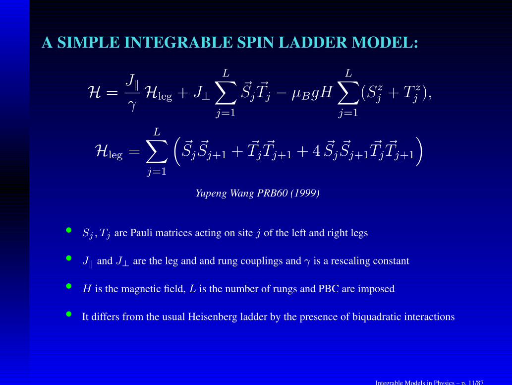
A SIMPLE INTEGRABLE SPIN LADDER MODEL:
H =J‖γ
Hleg + J⊥
L∑
j=1
~Sj ~Tj − µBgHL∑
j=1
(Szj + T zj ),
Hleg =L∑
j=1
(
~Sj ~Sj+1 + ~Tj ~Tj+1 + 4 ~Sj ~Sj+1~Tj ~Tj+1
)
Yupeng Wang PRB60 (1999)
• Sj , Tj are Pauli matrices acting on site j of the left and right legs
• J‖ and J⊥ are the leg and and rung couplings and γ is a rescaling constant
• H is the magnetic field, L is the number of rungs and PBC are imposed
• It differs from the usual Heisenberg ladder by the presence of biquadratic interactions
Integrable Models in Physics – p. 11/87
Properties:
• this model can be exactly solved by the BA:
the leg part is simply the permutation operator corresponding to the su(4) algebra and the
rung term becomes diagonal after a convenient change of basis;
• the gap and critical fields can be derived using the TBA;
• the thermal and magnetic properties can be obtained using
the Quantum Transfer Matrix (QTM) method:
the free energy is written in terms of the eigenvalue of the QTM and from it we derive the
thermodynamical properties by standard thermodynamics;
• this integrable ladder model can be used to describe the
physics of some strong coupling ladder compounds.
Integrable Models in Physics – p. 12/87
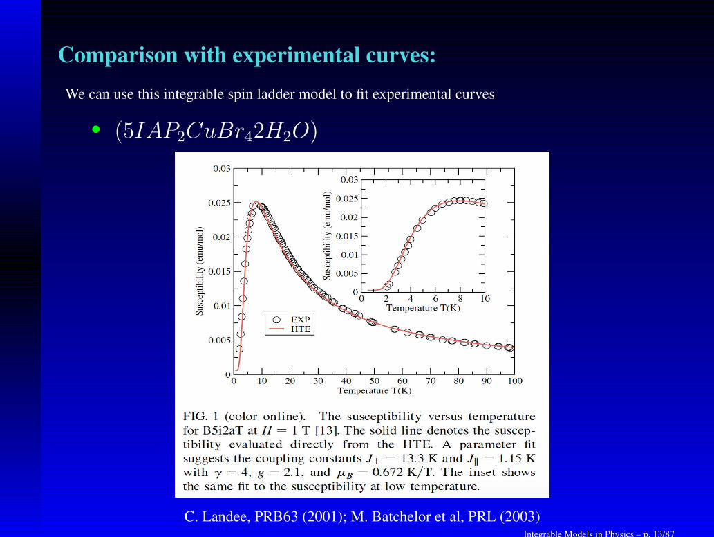
Comparison with experimental curves:
We can use this integrable spin ladder model to fit experimental curves
• (5IAP2CuBr42H2O)
C. Landee, PRB63 (2001); M. Batchelor et al, PRL (2003)Integrable Models in Physics – p. 13/87
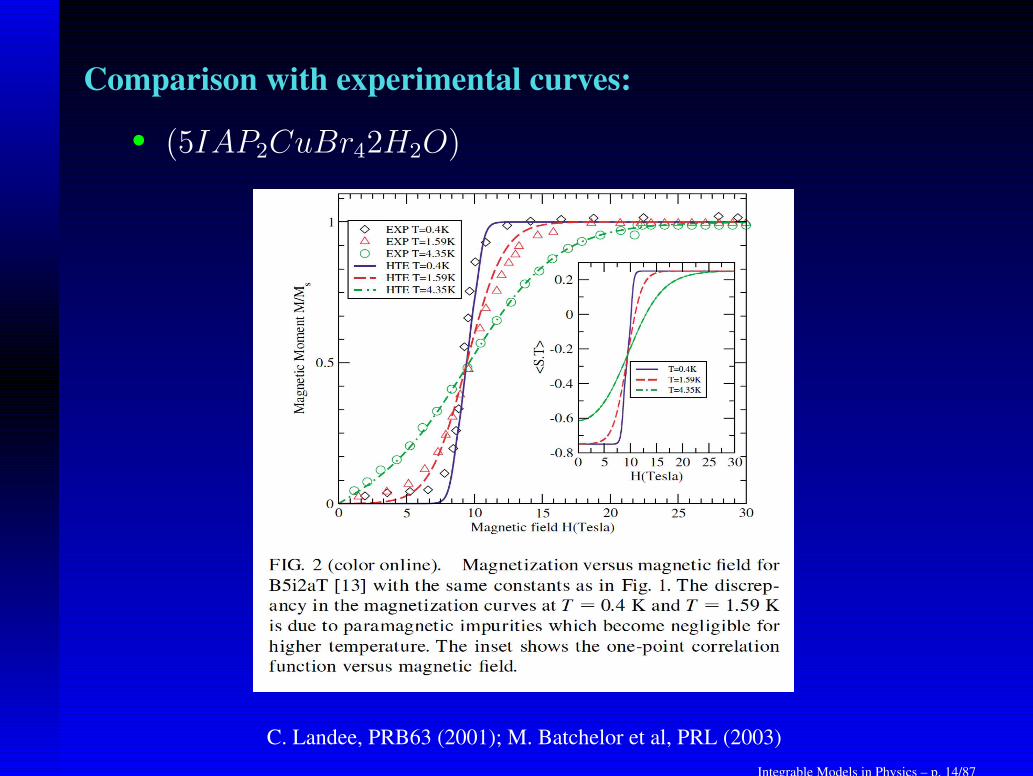
Comparison with experimental curves:
• (5IAP2CuBr42H2O)
C. Landee, PRB63 (2001); M. Batchelor et al, PRL (2003)
Integrable Models in Physics – p. 14/87
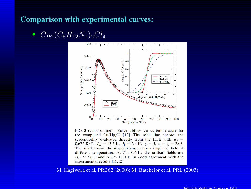
Comparison with experimental curves:
• Cu2(C5H12N2)2Cl4
M. Hagiwara et al, PRB62 (2000); M. Batchelor et al, PRL (2003)
Integrable Models in Physics – p. 15/87
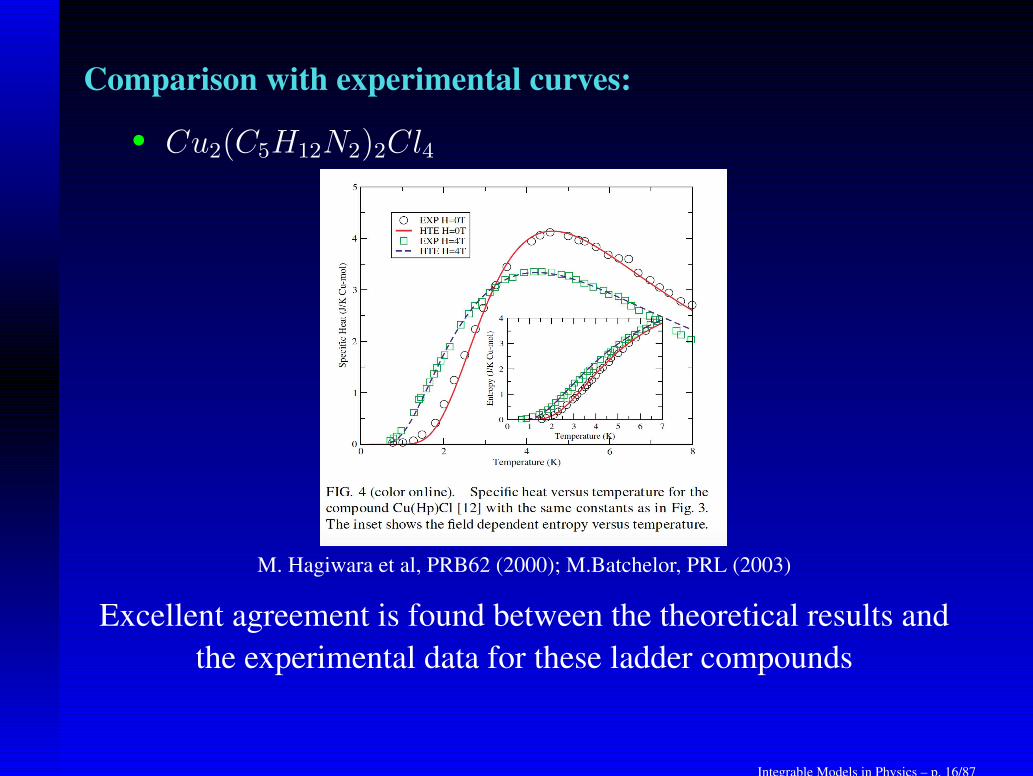
Comparison with experimental curves:
• Cu2(C5H12N2)2Cl4
M. Hagiwara et al, PRB62 (2000); M.Batchelor, PRL (2003)
Excellent agreement is found between the theoretical results and
the experimental data for these ladder compounds
Integrable Models in Physics – p. 16/87
Other integrable models in Condensed Matter
• Heisenberg chain
• Susy t-J model
• Hubbard model
• Kondo lattice and other impurity models
• . . .
Integrable Models in Physics – p. 17/87

3 - Integrable models in UltracoldMatter
Integrable Models in Physics – p. 18/87
Bosonic quantum tunneling models:
• 2 wells: Two-site Bose Hubbard Hamiltonian
• 3 wells: Triple well Hamiltonian
• 4 wells: Four-well ring model
• .......
• Multi-well tunneling models
Integrable Models in Physics – p. 19/87
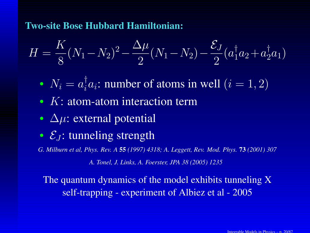
Two-site Bose Hubbard Hamiltonian:
H =K
8(N1−N2)
2−∆µ
2(N1−N2)−
EJ2(a†1a2+a
†2a1)
• Ni = a†iai: number of atoms in well (i = 1, 2)
• K: atom-atom interaction term
• ∆µ: external potential
• EJ : tunneling strengthG. Milburn et al, Phys. Rev. A 55 (1997) 4318; A. Leggett, Rev. Mod. Phys. 73 (2001) 307
A. Tonel, J. Links, A. Foerster, JPA 38 (2005) 1235
The quantum dynamics of the model exhibits tunneling X
self-trapping - experiment of Albiez et al - 2005
Integrable Models in Physics – p. 20/87
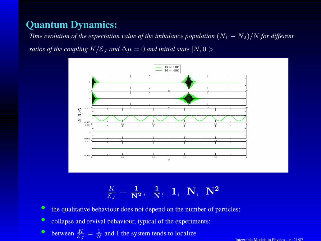
Quantum Dynamics:Time evolution of the expectation value of the imbalance population (N1 −N2)/N for different
ratios of the coupling K/EJ and ∆µ = 0 and initial state |N, 0 >
0 5 10 15 20-1
0
1
N = 100N = 400
0 5 10 15 20-1
0
1
0 0.2 0.4 0.6 0.8 10.999
1
1.001
<N1-N
2>/N
0 0.2 0.4 0.6 0.8 10.999
1
1.001
0 0.2 0.4 0.6 0.8 1
t0.999
1
1.001
KEJ = 1
N2 ,1
N, 1, N, N
2
• the qualitative behaviour does not depend on the number of particles;
• collapse and revival behaviour, typical of the experiments;
• between KEJ
= 1N
and 1 the system tends to localizeIntegrable Models in Physics – p. 21/87
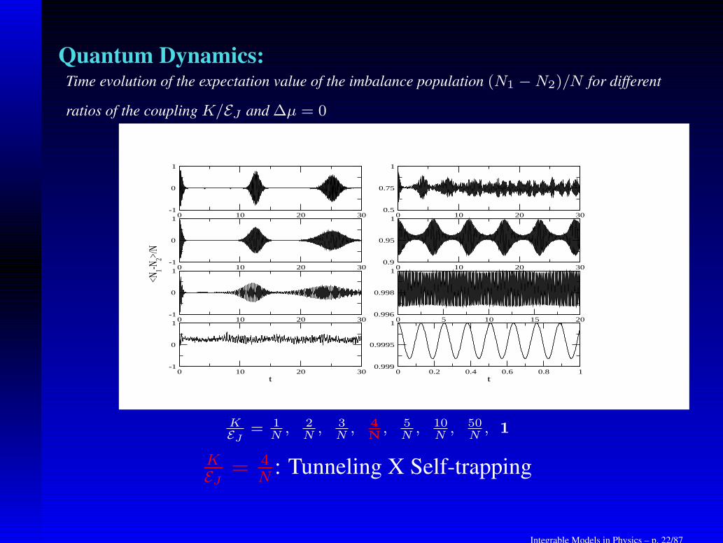
Quantum Dynamics:Time evolution of the expectation value of the imbalance population (N1 −N2)/N for different
ratios of the coupling K/EJ and ∆µ = 0
0 10 20 30-1
0
1
0 10 20 300.5
0.75
1
0 10 20 30-1
0
1
0 10 20 300.9
0.95
1
0 10 20 30-1
0
1
<N1-N
2>/N
0 5 10 15 200.996
0.998
1
0 10 20 30t
-1
0
1
0 0.2 0.4 0.6 0.8 1t
0.999
0.9995
1
KEJ
= 1N, 2
N, 3
N, 4
N, 5
N, 10
N, 50
N, 1
KEJ = 4
N: Tunneling X Self-trapping
Integrable Models in Physics – p. 22/87
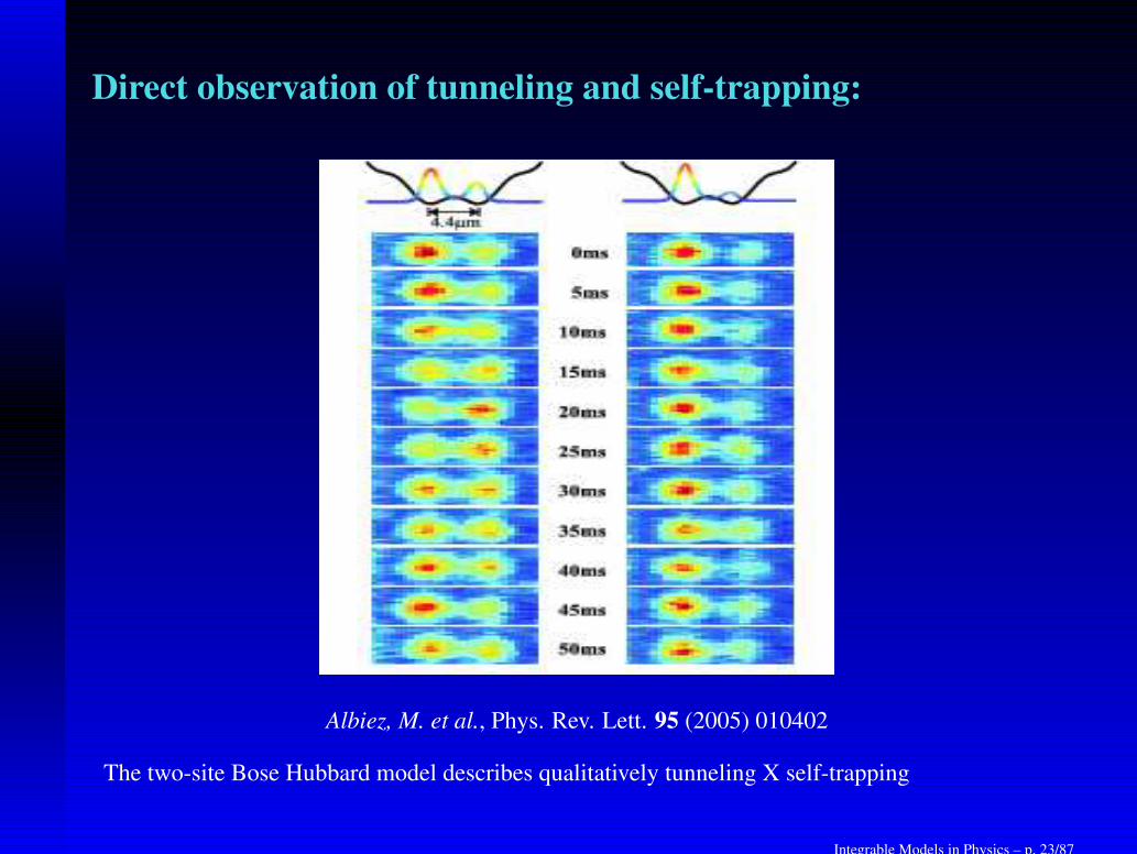
Direct observation of tunneling and self-trapping:
Albiez, M. et al., Phys. Rev. Lett. 95 (2005) 010402
The two-site Bose Hubbard model describes qualitatively tunneling X self-trapping
Integrable Models in Physics – p. 23/87
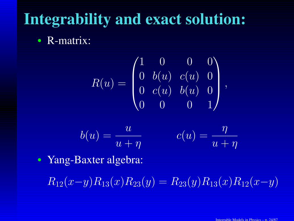
Integrability and exact solution:• R-matrix:
R(u) =
1 0 0 0
0 b(u) c(u) 0
0 c(u) b(u) 0
0 0 0 1
,
b(u) =u
u+ ηc(u) =
η
u+ η
• Yang-Baxter algebra:
R12(x−y)R13(x)R23(y) = R23(y)R13(x)R12(x−y)
Integrable Models in Physics – p. 24/87
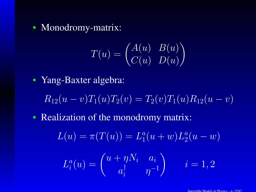
• Monodromy-matrix:
T (u) =
(
A(u) B(u)
C(u) D(u)
)
• Yang-Baxter algebra:
R12(u− v)T1(u)T2(v) = T2(v)T1(u)R12(u− v)
• Realization of the monodromy matrix:
L(u) = π(T (u)) = La1(u+ w)La
2(u− w)
Lai (u) =
(
u+ ηNi aia†i η−1
)
i = 1, 2
Integrable Models in Physics – p. 25/87
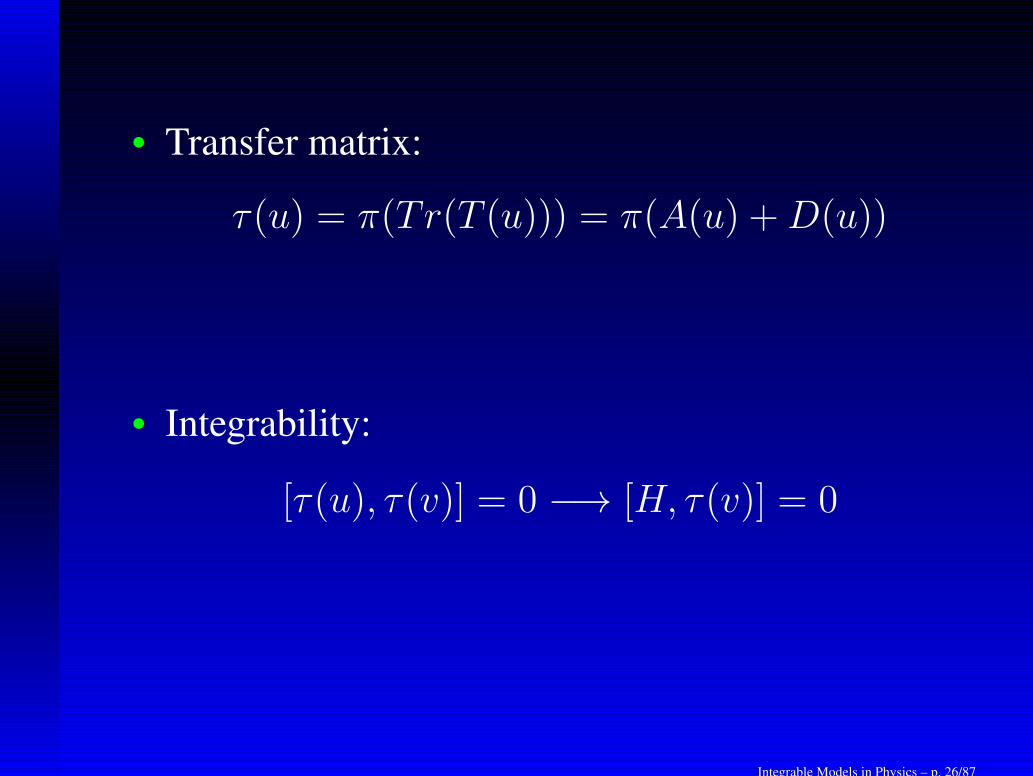
• Transfer matrix:
τ(u) = π(Tr(T (u))) = π(A(u) +D(u))
• Integrability:
[τ(u), τ(v)] = 0 −→ [H, τ(v)] = 0
Integrable Models in Physics – p. 26/87
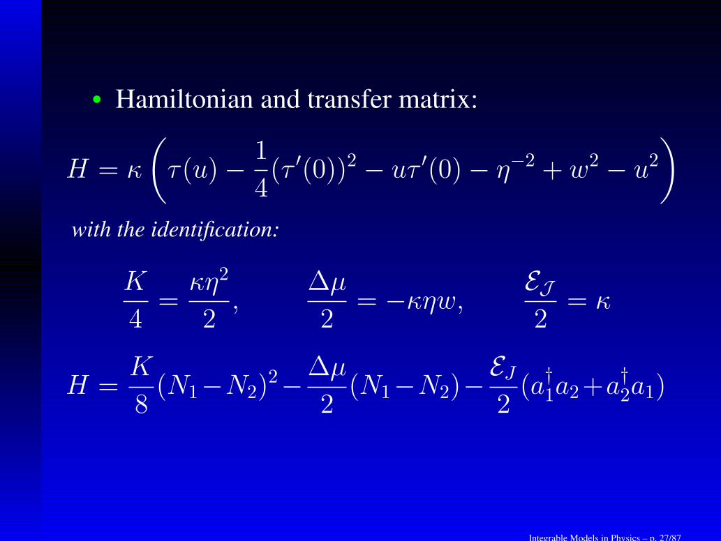
• Hamiltonian and transfer matrix:
H = κ
(
τ(u)− 1
4(τ ′(0))2 − uτ ′(0)− η−2 + w2 − u2
)
with the identification:
K
4=κη2
2,
∆µ
2= −κηw, EJ
2= κ
H =K
8(N1−N2)
2−∆µ
2(N1−N2)−
EJ2(a†1a2+a
†2a1)
Integrable Models in Physics – p. 27/87
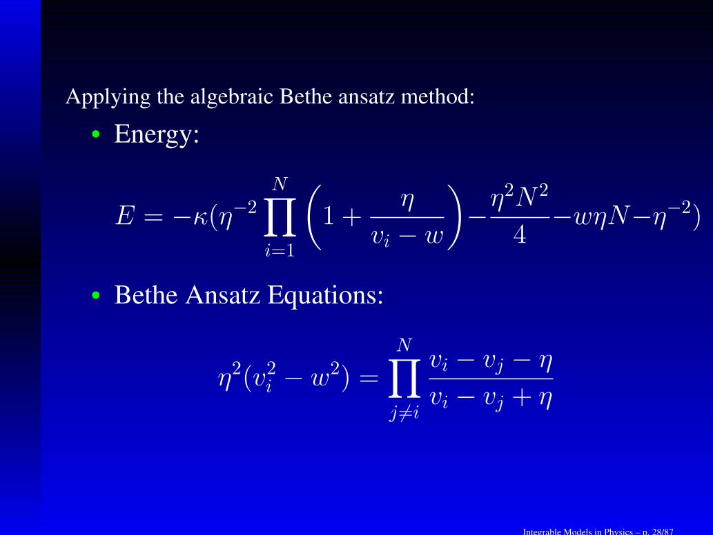
Applying the algebraic Bethe ansatz method:
• Energy:
E = −κ(η−2
N∏
i=1
(
1 +η
vi − w
)
−η2N 2
4−wηN−η−2)
• Bethe Ansatz Equations:
η2(v2i − w2) =N∏
j 6=i
vi − vj − η
vi − vj + η
Integrable Models in Physics – p. 28/87
INTEGRABLE GENERALISED MODELS:
Basic idea:
We can construct integrable generalised modelsin this bosonic quantum tunneling context byexploring different representations of somealgebra.
A. Foerster and E. Ragoucy, Nuclear Phys. B777 (2007) 373
A. Tonel, L. Ymai, A. Foerster and J. Links, J. Phys. A48 (2015)
L. Ymai, A. Tonel, A. Foerster and J. Links, arXiv:1606.00816 (2016)
Integrable Models in Physics – p. 29/87
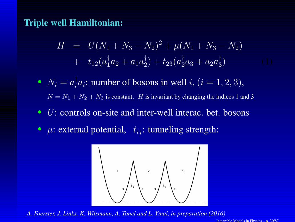
Triple well Hamiltonian:
H = U(N1 +N3 −N2)2 + µ(N1 +N3 −N2)
+ t12(a†1a2 + a1a
†2) + t23(a
†2a3 + a2a
†3) (1)
• Ni = a†iai: number of bosons in well i, (i = 1, 2, 3),
N = N1 +N2 +N3 is constant, H is invariant by changing the indices 1 and 3
• U : controls on-site and inter-well interac. bet. bosons
• µ: external potential, tij: tunneling strength:
A. Foerster, J. Links, K. Wilsmann, A. Tonel and L. Ymai, in preparation (2016)Integrable Models in Physics – p. 30/87
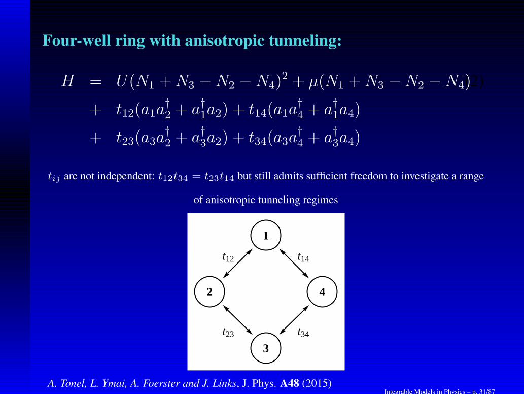
Four-well ring with anisotropic tunneling:
H = U(N1 +N3 −N2 −N4)2 + µ(N1 +N3 −N2 −N4)(2)
+ t12(a1a†2 + a†1a2) + t14(a1a
†4 + a†1a4)
+ t23(a3a†2 + a†3a2) + t34(a3a
†4 + a†3a4)
tij are not independent: t12t34 = t23t14 but still admits sufficient freedom to investigate a range
of anisotropic tunneling regimes
1
2
3
4
t14
t23
t12
t34
A. Tonel, L. Ymai, A. Foerster and J. Links, J. Phys. A48 (2015)Integrable Models in Physics – p. 31/87
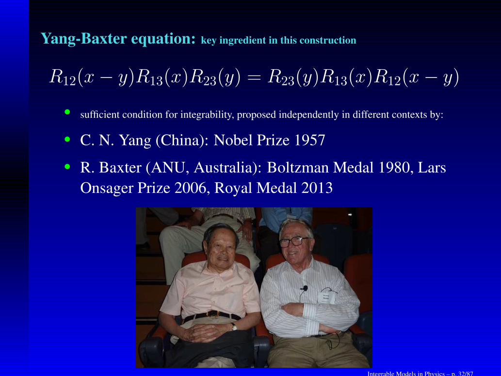
Yang-Baxter equation: key ingredient in this construction
R12(x− y)R13(x)R23(y) = R23(y)R13(x)R12(x− y)
• sufficient condition for integrability, proposed independently in different contexts by:
• C. N. Yang (China): Nobel Prize 1957
• R. Baxter (ANU, Australia): Boltzman Medal 1980, Lars
Onsager Prize 2006, Royal Medal 2013
Integrable Models in Physics – p. 32/87
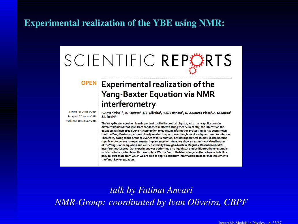
Experimental realization of the YBE using NMR:
talk by Fatima Anvari
NMR-Group: coordinated by Ivan Oliveira, CBPF
Integrable Models in Physics – p. 33/87

Ultracold Fermi gases
Integrable Models in Physics – p. 34/87
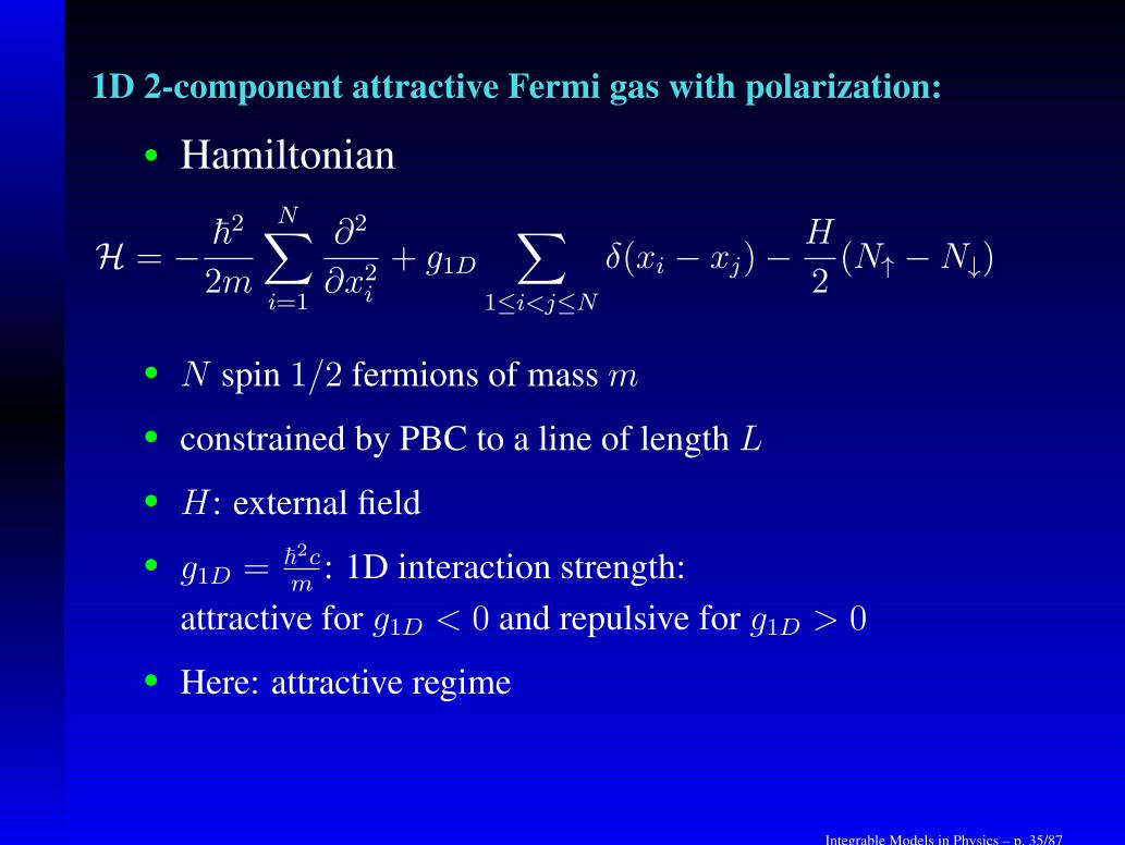
1D 2-component attractive Fermi gas with polarization:
• Hamiltonian
H = − ~2
2m
N∑
i=1
∂2
∂x2i+ g1D
∑
1≤i<j≤Nδ(xi − xj)−
H
2(N↑ −N↓)
• N spin 1/2 fermions of mass m
• constrained by PBC to a line of length L
• H: external field
• g1D = ~2cm
: 1D interaction strength:
attractive for g1D < 0 and repulsive for g1D > 0
• Here: attractive regime
Integrable Models in Physics – p. 35/87
Properties:
• this model can be exactly solved by the BA
C.N. Yang, PRL 19(1967)1312; M. Gaudin, Phys. Lett. 24 (1967) 55
• using the TBA we can derive thermodynamical properties
and also obtain the phase diagram for strong and weak
coupling.
• using the TBA, we can also obtain the Wilson ratio RW , an
universal quantity defined as the ratio of the magnetic
susceptibility χ to specific heat cv divided by T ( in the
strong attractive and low T regime)
RW ∝ χ
cv/T
Integrable Models in Physics – p. 36/87
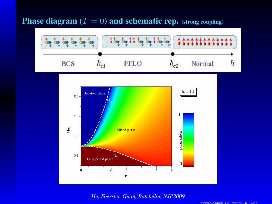
Phase diagram (T = 0) and schematic rep. (strong coupling)
He, Foerster, Guan, Batchelor, NJP2009Integrable Models in Physics – p. 37/87
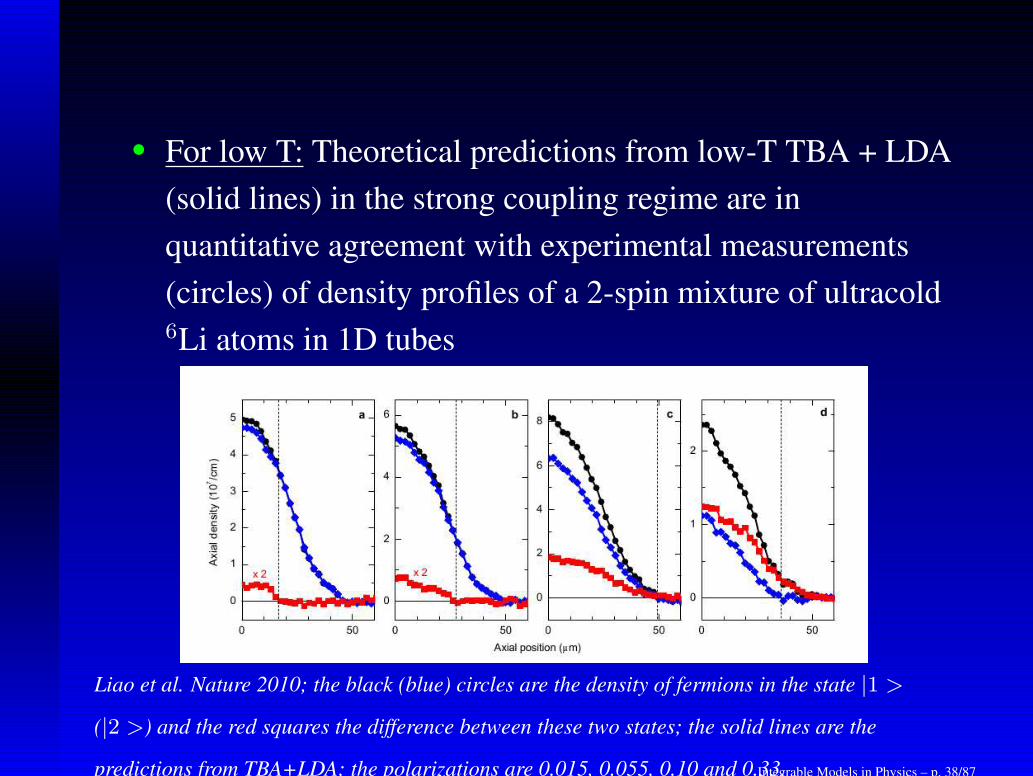
• For low T: Theoretical predictions from low-T TBA + LDA
(solid lines) in the strong coupling regime are in
quantitative agreement with experimental measurements
(circles) of density profiles of a 2-spin mixture of ultracold6Li atoms in 1D tubes
Liao et al. Nature 2010; the black (blue) circles are the density of fermions in the state |1 >
(|2 >) and the red squares the difference between these two states; the solid lines are the
predictions from TBA+LDA; the polarizations are 0.015, 0.055, 0.10 and 0.33.Integrable Models in Physics – p. 38/87
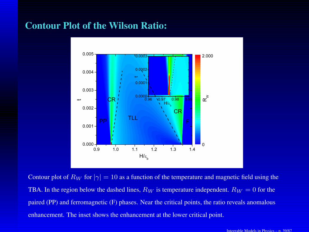
Contour Plot of the Wilson Ratio:
0.9 1.0 1.1 1.2 1.3 1.40.000
0.001
0.002
0.003
0.004
0.005
H/b
t
RW
CR
CR
FPP TLL
H/ b
0
2.000
0.96 0.97 0.98 0.990.0000
0.0001
0.0002
0.0003
t
Contour plot of RW for |γ| = 10 as a function of the temperature and magnetic field using the
TBA. In the region below the dashed lines, RW is temperature independent. RW = 0 for the
paired (PP) and ferromagnetic (F) phases. Near the critical points, the ratio reveals anomalous
enhancement. The inset shows the enhancement at the lower critical point.
Integrable Models in Physics – p. 39/87
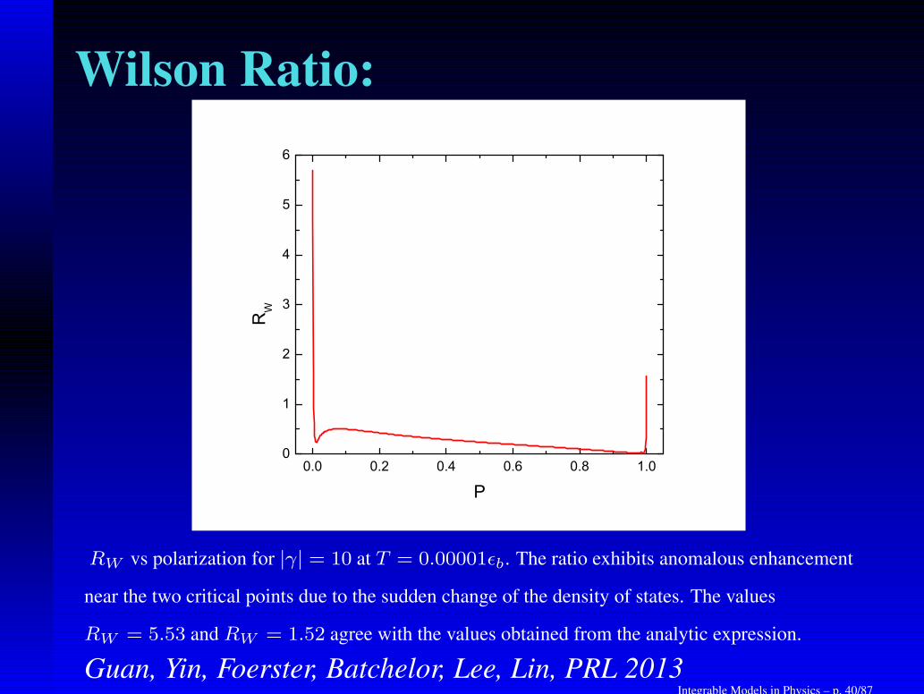
Wilson Ratio:
0.0 0.2 0.4 0.6 0.8 1.00
1
2
3
4
5
6
RW
P
RW vs polarization for |γ| = 10 at T = 0.00001ǫb. The ratio exhibits anomalous enhancement
near the two critical points due to the sudden change of the density of states. The values
RW = 5.53 and RW = 1.52 agree with the values obtained from the analytic expression.
Guan, Yin, Foerster, Batchelor, Lee, Lin, PRL 2013Integrable Models in Physics – p. 40/87
Other integrable models in Ultracold Matter
Advanced experimental techniques in trapping and cooling atoms in 1D have provided the
realization of integrable models in the lab. Some examples:
• the Lieb-Liniger Bose gasT. Kinoshita et al Science 2004, PRL 2005, Nature 2006; A. van Amerongen et al
PRL2008; T. Kitagawa et al PRL 2010; J. Armijo et al PRL 2010, H. Naegerl et al, 2015
• the super Tonks-Girardeau gasE. Haller et al Science 2009
• the two-component spinor Bose gasJ. van Druten et al arXiv:1010.4545
• McGuire impurity model in 1D Fermi gasS. Jochim et al, Science 2011, PRL 2012, Science 2013.
Integrable Models in Physics – p. 41/87

• Even if a system is not integrablewe can get inspiration from these methods;
• We can see this, for instance in the case of fewparticles systems, which are attracting greatinterest due to recent experiments in cold atoms.
Integrable Models in Physics – p. 42/87

Few particles
Integrable Models in Physics – p. 43/87

Few Particles System:• Very recent experiments: Jochim et al prepared and controlled with high precision a
system of few 6Li atoms (N) in a 1D harmonic trap - Science 2012
Microtrap + tilting the potential
Combining the Bethe ansatz + variational principle we discuss few particles system
Integrable Models in Physics – p. 44/87
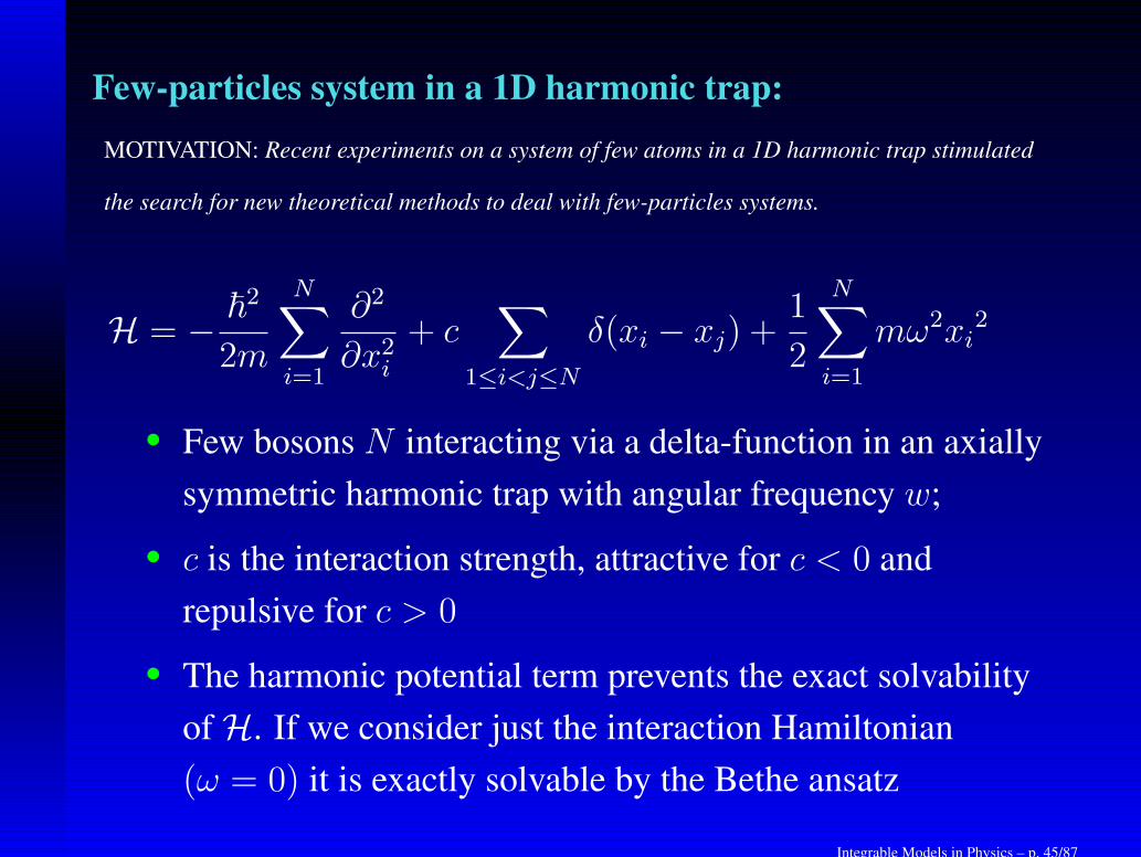
Few-particles system in a 1D harmonic trap:
MOTIVATION: Recent experiments on a system of few atoms in a 1D harmonic trap stimulated
the search for new theoretical methods to deal with few-particles systems.
H = − ~2
2m
N∑
i=1
∂2
∂x2i+ c
∑
1≤i<j≤Nδ(xi − xj) +
1
2
N∑
i=1
mω2xi2
• Few bosons N interacting via a delta-function in an axially
symmetric harmonic trap with angular frequency w;
• c is the interaction strength, attractive for c < 0 and
repulsive for c > 0
• The harmonic potential term prevents the exact solvability
of H. If we consider just the interaction Hamiltonian
(ω = 0) it is exactly solvable by the Bethe ansatz
Integrable Models in Physics – p. 45/87
H = − ~2
2m
N∑
i=1
∂2
∂x2i+ g1D
∑
1≤i<j≤Nδ(xi − xj) +
1
2
N∑
i=1
mω2xi2
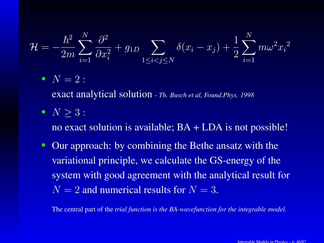
• N = 2 :
exact analytical solution - Th. Busch et al, Found.Phys. 1998
• N ≥ 3 :
no exact solution is available; BA + LDA is not possible!
• Our approach: by combining the Bethe ansatz with the
variational principle, we calculate the GS-energy of the
system with good agreement with the analytical result for
N = 2 and numerical results for N = 3.
The central part of the trial function is the BA-wavefunction for the integrable model.
Integrable Models in Physics – p. 46/87
Ground state energies:
N=2Geometric
Analytic
N=3Geometric
Numeric
-5 0 5 10 15 20-2.0
-1.5
-1.0
-0.5
0.0
0.5
1.0
c
Ε
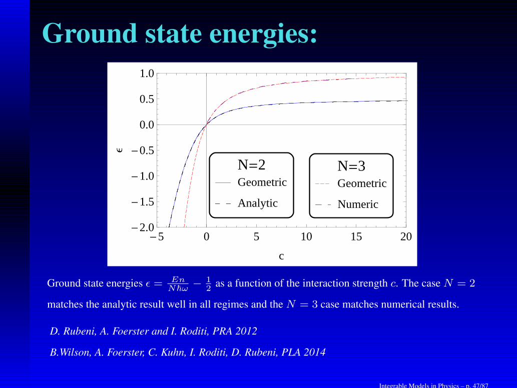
Ground state energies ǫ = EnN~ω
− 12
as a function of the interaction strength c. The case N = 2
matches the analytic result well in all regimes and the N = 3 case matches numerical results.
D. Rubeni, A. Foerster and I. Roditi, PRA 2012
B.Wilson, A. Foerster, C. Kuhn, I. Roditi, D. Rubeni, PLA 2014
Integrable Models in Physics – p. 47/87
Probability density for N = 2:
0.0
0.2
0.4
0.6
0.8
ÈΨHΛLÈ
2
HaL HbL HcL
-4 -2 0 2 40.0
0.2
0.4
0.6
0.8
r1
ÈΨHΛLÈ
2
HdL
-4 -2 0 2 4
r1
HeL
-4 -2 0 2 4
r1
HfL Geometric
Analytic
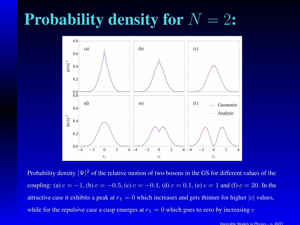
Probability density |Ψ|2 of the relative motion of two bosons in the GS for different values of the
coupling: (a) c = −1, (b) c = −0.5, (c) c = −0.1, (d) c = 0.1, (e) c = 1 and (f) c = 20. In the
attractive case it exhibits a peak at r1 = 0 which increases and gets thinner for higher |c| values,
while for the repulsive case a cusp emerges at r1 = 0 which goes to zero by increasing c
Integrable Models in Physics – p. 48/87
Probability density for N = 3:
-4
-2
0
2
4
r 2
HaL
-4
-2
0
2
4
r 2
HaL HbLHbL HcLHcL
-4 -2 0 2 4r1
-4
-2
0
2
4
r 2
HdL
-4 -2 0 2 4r1
-4
-2
0
2
4
r 2
HdL
-4 -2 0 2 4r1
HeL
-4 -2 0 2 4r1
HeL
-4 -2 0 2 4r1
Hf L
-4 -2 0 2 4r1
Hf L
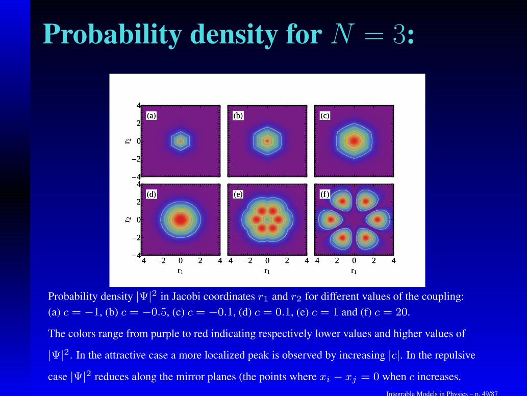
Probability density |Ψ|2 in Jacobi coordinates r1 and r2 for different values of the coupling:
(a) c = −1, (b) c = −0.5, (c) c = −0.1, (d) c = 0.1, (e) c = 1 and (f) c = 20.
The colors range from purple to red indicating respectively lower values and higher values of
|Ψ|2. In the attractive case a more localized peak is observed by increasing |c|. In the repulsive
case |Ψ|2 reduces along the mirror planes (the points where xi − xj = 0 when c increases.
Integrable Models in Physics – p. 49/87
Pair correlations:
-2
-1
0
1
2
x 2
HaL HbL HcL
-2 -1 0 1 2-2
-1
0
1
2
x1
x 2
HdL
-2 -1 0 1 2
x1
HeL
-2 -1 0 1 2
x1
Hf L
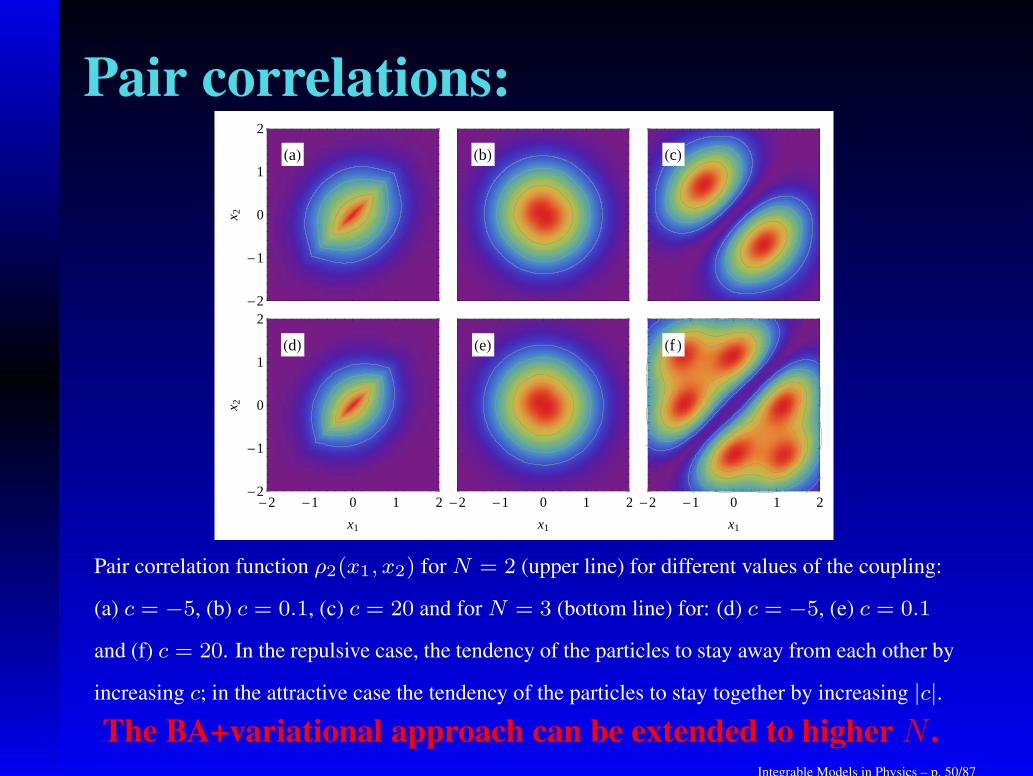
Pair correlation function ρ2(x1, x2) for N = 2 (upper line) for different values of the coupling:
(a) c = −5, (b) c = 0.1, (c) c = 20 and for N = 3 (bottom line) for: (d) c = −5, (e) c = 0.1
and (f) c = 20. In the repulsive case, the tendency of the particles to stay away from each other by
increasing c; in the attractive case the tendency of the particles to stay together by increasing |c|.
The BA+variational approach can be extended to higher N .Integrable Models in Physics – p. 50/87

4- BREAKING THEINTEGRABILITY
Integrable Models in Physics – p. 51/87
Breakdown of the integrability: Heisenberg chain
• The transport behavior in the integrable system contrasts
with the non-integrable or chaotic chain, suggesting
ballistic transport (integrable case) X diffusive transport
(chaotic case).
• See also related work:
M. Haque, D. Luitz, S. Mukerjee, H. Pastawski, R. Pereira,
A. Polkovnikov, F. Pollmann, T. Prosen, J. Sirker
Integrable Models in Physics – p. 52/87
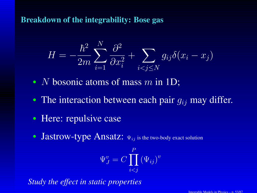
Breakdown of the integrability: Bose gas
H = − ~2
2m
N∑
i=1
∂2
∂x2i+
∑
i<j≤N
gijδ(xi − xj)
• N bosonic atoms of mass m in 1D;
• The interaction between each pair gij may differ.
• Here: repulsive case
• Jastrow-type Ansatz: Ψij is the two-body exact solution
ΨvJ = C
P∏
i<j
(Ψij)v
Study the effect in static propertiesIntegrable Models in Physics – p. 53/87
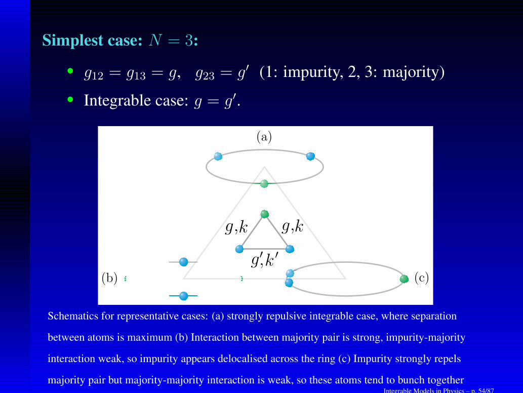
Simplest case: N = 3:
• g12 = g13 = g, g23 = g′ (1: impurity, 2, 3: majority)
• Integrable case: g = g′.
Schematics for representative cases: (a) strongly repulsive integrable case, where separation
between atoms is maximum (b) Interaction between majority pair is strong, impurity-majority
interaction weak, so impurity appears delocalised across the ring (c) Impurity strongly repels
majority pair but majority-majority interaction is weak, so these atoms tend to bunch togetherIntegrable Models in Physics – p. 54/87
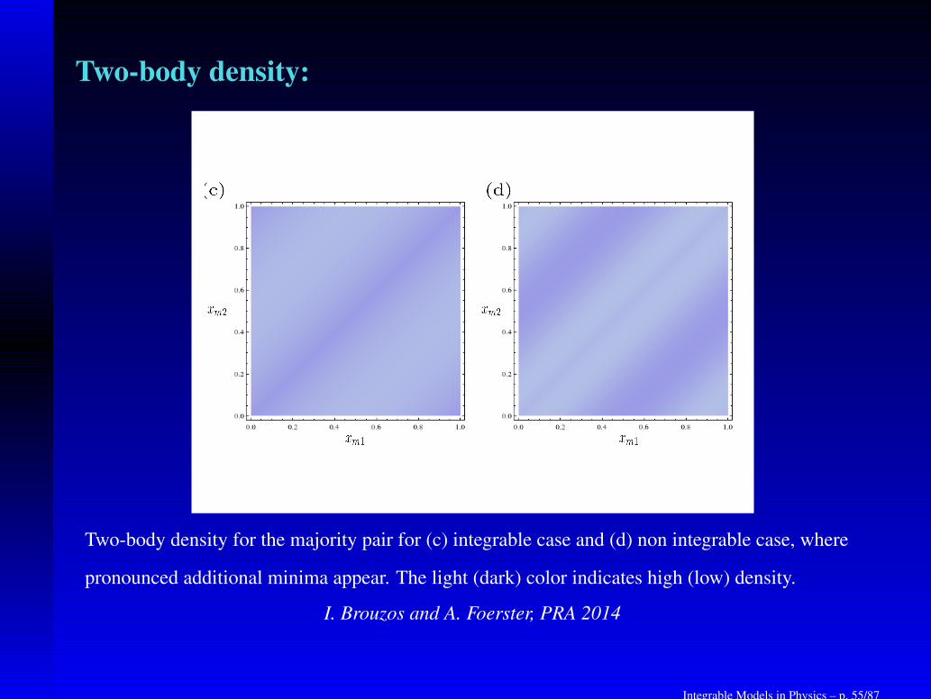
Two-body density:
Two-body density for the majority pair for (c) integrable case and (d) non integrable case, where
pronounced additional minima appear. The light (dark) color indicates high (low) density.
I. Brouzos and A. Foerster, PRA 2014
Integrable Models in Physics – p. 55/87
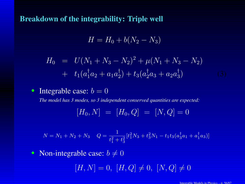
Breakdown of the integrability: Triple well
H = H0 + b(N2 −N3)
H0 = U(N1 +N3 −N2)2 + µ(N1 +N3 −N2)
+ t1(a†1a2 + a1a
†2) + t3(a
†2a3 + a2a
†3) (3)
• Integrable case: b = 0The model has 3 modes, so 3 independent conserved quantities are expected:
[H0, N ] = [H0, Q] = [N,Q] = 0
N = N1 +N2 +N3 Q =1
t21 + t23[t21N3 + t23N1 − t1t3(a
†3a1 + a†1a3)]
• Non-integrable case: b 6= 0
[H,N ] = 0, [H,Q] 6= 0, [N,Q] 6= 0
Integrable Models in Physics – p. 56/87
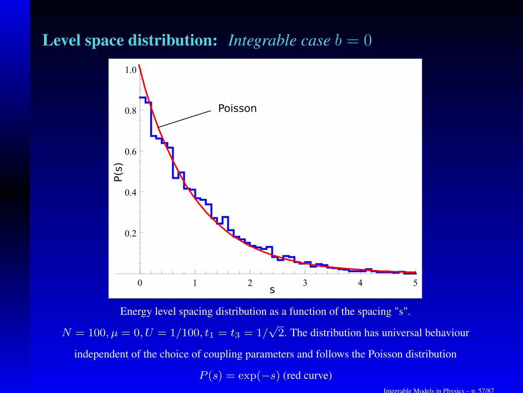
Level space distribution: Integrable case b = 0
Energy level spacing distribution as a function of the spacing "s".
N = 100, µ = 0, U = 1/100, t1 = t3 = 1/√2. The distribution has universal behaviour
independent of the choice of coupling parameters and follows the Poisson distribution
P (s) = exp(−s) (red curve)
Integrable Models in Physics – p. 57/87
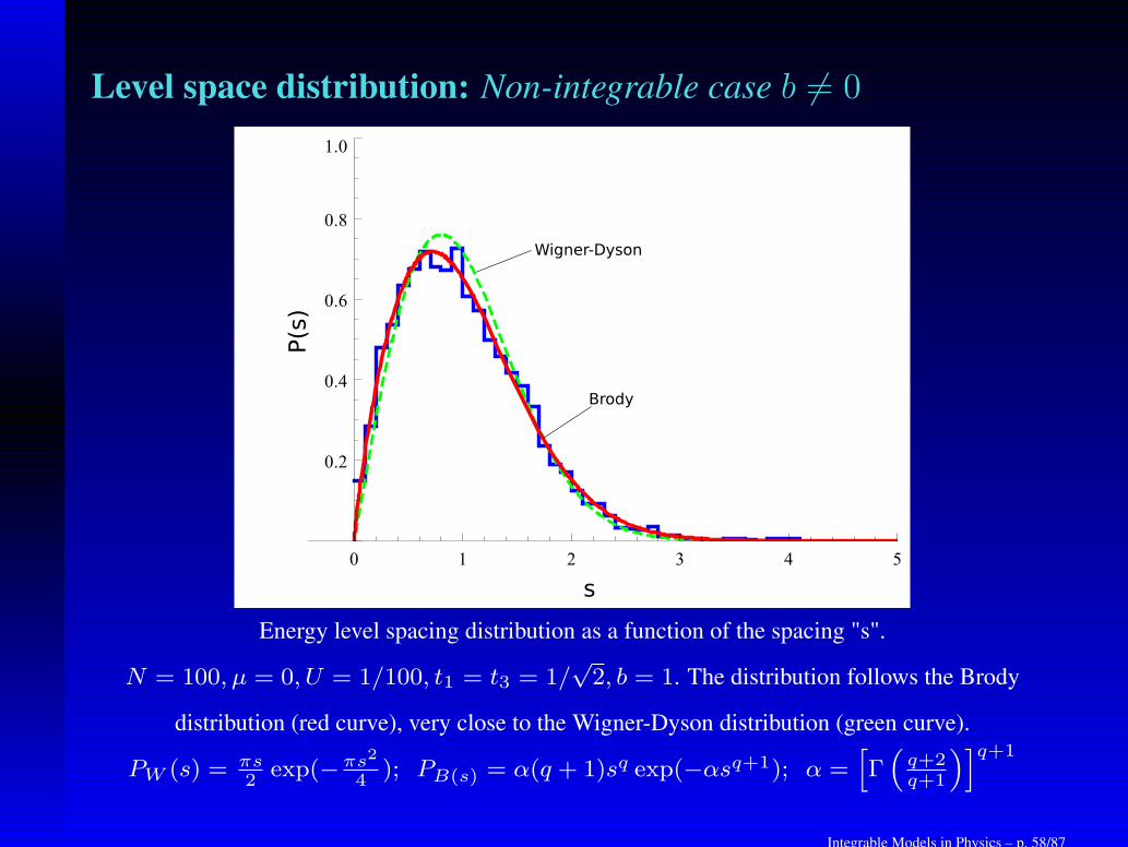
Level space distribution: Non-integrable case b 6= 0
Energy level spacing distribution as a function of the spacing "s".
N = 100, µ = 0, U = 1/100, t1 = t3 = 1/√2, b = 1. The distribution follows the Brody
distribution (red curve), very close to the Wigner-Dyson distribution (green curve).
PW (s) = πs2
exp(−πs2
4); PB(s) = α(q + 1)sq exp(−αsq+1); α =
[
Γ(
q+2q+1
)]q+1
Integrable Models in Physics – p. 58/87

5- CONCLUDING REMARKS
Integrable Models in Physics – p. 59/87

Concluding remarks:• We have presented some examples in which integrable
models are relevant. This list should be considered
remarkable, not necessarily because of the examples given,
but arguably also because of what has been omitted.
• There are a wealth of integrable models which are yet to
find their way into experiments.
• It is clear that integrable models will continue to offer
valuable insights into the description of physical properties
and experimental results for decades to come.
Integrable Models in Physics – p. 60/87
Collaborators1. Prof. Murray T. Batchelor, ANU-Australia
2. Prof. Jon Links, UQ-QLD-Australia
3. Prof. Xi-Wen Guan, Wuhan-China
4. * Prof. Ivan S. Oliveira, CBPF-Brazil
5. Prof. Itzhak Roditi, CBPF-Brazil
6. Prof. Arlei Tonel, Unipampa-Brazil
7. Prof. Leandro Yimai, Unipampa-Brazil
8. Prof. Nikolaj T. Zinner, Aarhus University, Denmark
9. Dr. Ioannis Brouzos
10. Dr. Carlos Kuhn, ANU-Australia
11. Dr. Diefferson Lima, UQ-QLD-Australia
12. Dr. Brendan Wilson, ANU-Australia
13. * Dr. Fatima Anvari, (post-doc), UFRGS-Brazil
14. Rafael Barfknecht (PHd student), UFRGS-Brazil
15. David Carvalho (PHd student), UFRGS-Brazil
16. Karin Wilsmann (Master student), UFRGS-Brazil
Integrable Models in Physics – p. 61/87

Integrable Models in Physics – p. 62/87
Integrability: Formal definition
It is generally accepted that an integrable system is one which is
derived from a set of commuting transfer matrices.
This definition applies to many-body systems.
Transfer matrix τ(u): is a generating function of conserved quantities
• The condition:
[τ(u), τ(v)] = 0
• represents (an infinite set of) conservation laws:
[cn, cm] = 0
• where the series expansion was taken:
τ =∑
n
cnvn
Integrable Models in Physics – p. 63/87
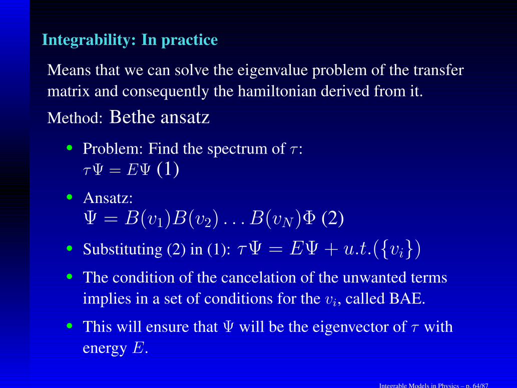
Integrability: In practice
Means that we can solve the eigenvalue problem of the transfer
matrix and consequently the hamiltonian derived from it.
Method: Bethe ansatz
• Problem: Find the spectrum of τ :
τΨ = EΨ (1)
• Ansatz:
Ψ = B(v1)B(v2) . . . B(vN)Φ (2)
• Substituting (2) in (1): τΨ = EΨ+ u.t.({vi})• The condition of the cancelation of the unwanted terms
implies in a set of conditions for the vi, called BAE.
• This will ensure that Ψ will be the eigenvector of τ with
energy E.
Integrable Models in Physics – p. 64/87
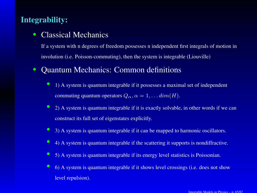
Integrability:
• Classical Mechanics
If a system with n degrees of freedom possesses n independent first integrals of motion in
involution (i.e. Poisson-commuting), then the system is integrable (Liouville)
• Quantum Mechanics: Common definitions
• 1) A system is quantum integrable if it possesses a maximal set of independent
commuting quantum operators Qα, α = 1, . . . dim(H).
• 2) A system is quantum integrable if it is exactly solvable, in other words if we can
construct its full set of eigenstates explicitly.
• 3) A system is quantum integrable if it can be mapped to harmonic oscillators.
• 4) A system is quantum integrable if the scattering it supports is nondiffractive.
• 5) A system is quantum integrable if its energy level statistics is Poissonian.
• 6) A system is quantum integrable if it shows level crossings (i.e. does not show
level repulsion).
Integrable Models in Physics – p. 65/87
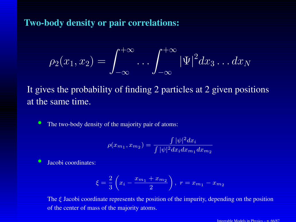
Two-body density or pair correlations:
ρ2(x1, x2) =
∫
+∞
−∞. . .
∫
+∞
−∞|Ψ|2dx3 . . . dxN
It gives the probability of finding 2 particles at 2 given positions
at the same time.
• The two-body density of the majority pair of atoms:
ρ(xm1, xm2
) =
∫
|ψ|2dxi∫
|ψ|2dxidxm1dxm2
• Jacobi coordinates:
ξ =2
3
(
xi −xm1
+ xm2
2
)
, r = xm1− xm2
The ξ Jacobi coordinate represents the position of the impurity, depending on the position
of the center of mass of the majority atoms.
Integrable Models in Physics – p. 66/87
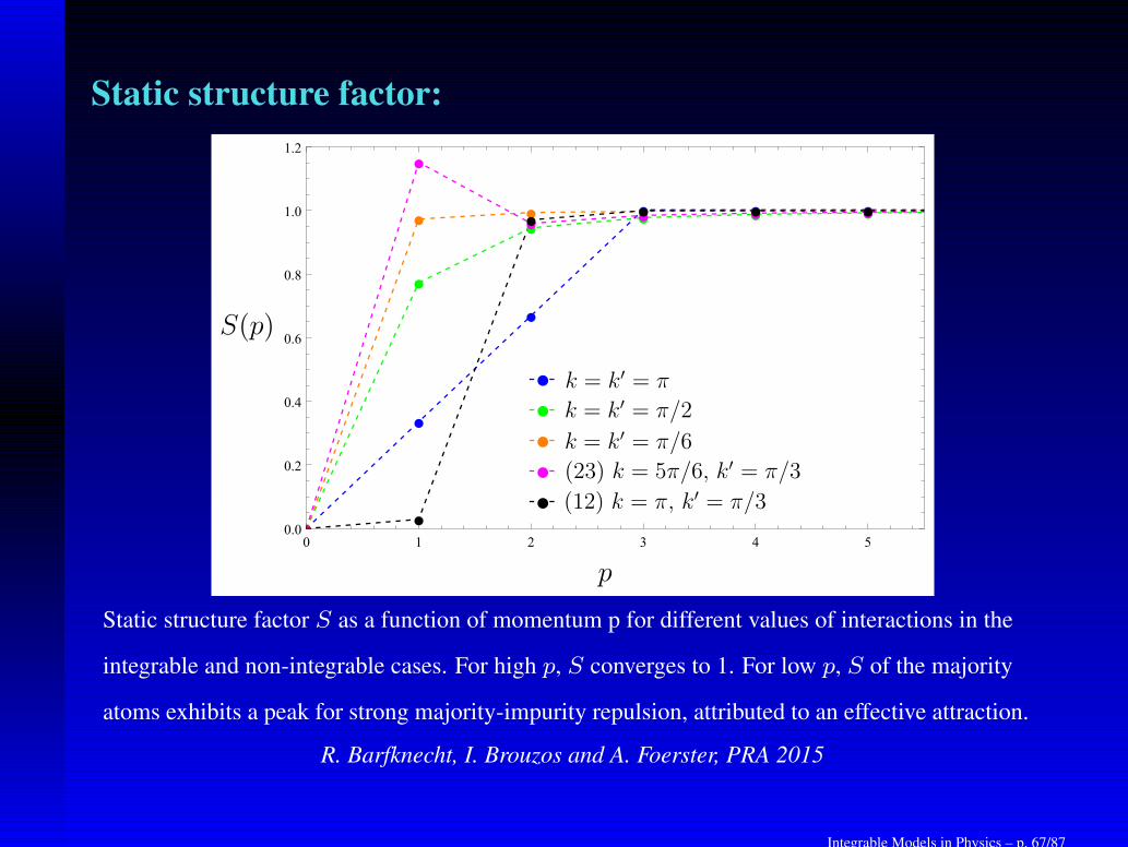
Static structure factor:
Static structure factor S as a function of momentum p for different values of interactions in the
integrable and non-integrable cases. For high p, S converges to 1. For low p, S of the majority
atoms exhibits a peak for strong majority-impurity repulsion, attributed to an effective attraction.
R. Barfknecht, I. Brouzos and A. Foerster, PRA 2015
Integrable Models in Physics – p. 67/87
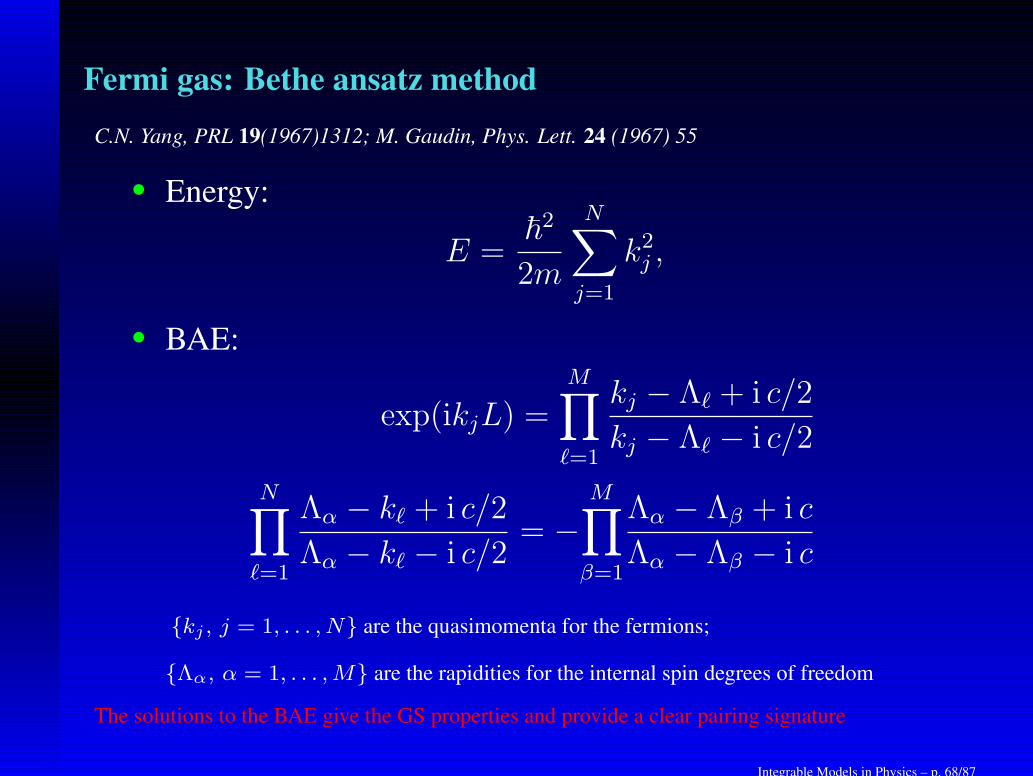
Fermi gas: Bethe ansatz method
C.N. Yang, PRL 19(1967)1312; M. Gaudin, Phys. Lett. 24 (1967) 55
• Energy:
E =~2
2m
N∑
j=1
k2j ,
• BAE:
exp(ikjL) =M∏
ℓ=1
kj − Λℓ + i c/2
kj − Λℓ − i c/2
N∏
ℓ=1
Λα − kℓ + i c/2
Λα − kℓ − i c/2= −
M∏
β=1
Λα − Λβ + i c
Λα − Λβ − i c
{kj , j = 1, . . . , N} are the quasimomenta for the fermions;
{Λα, α = 1, . . . ,M} are the rapidities for the internal spin degrees of freedom
The solutions to the BAE give the GS properties and provide a clear pairing signature
Integrable Models in Physics – p. 68/87
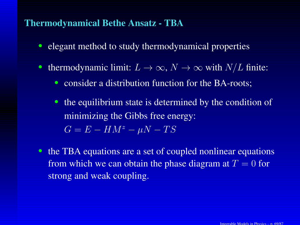
Thermodynamical Bethe Ansatz - TBA
• elegant method to study thermodynamical properties
• thermodynamic limit: L→ ∞, N → ∞ with N/L finite:
• consider a distribution function for the BA-roots;
• the equilibrium state is determined by the condition of
minimizing the Gibbs free energy:
G = E −HM z − µN − TS
• the TBA equations are a set of coupled nonlinear equations
from which we can obtain the phase diagram at T = 0 for
strong and weak coupling.
Integrable Models in Physics – p. 69/87
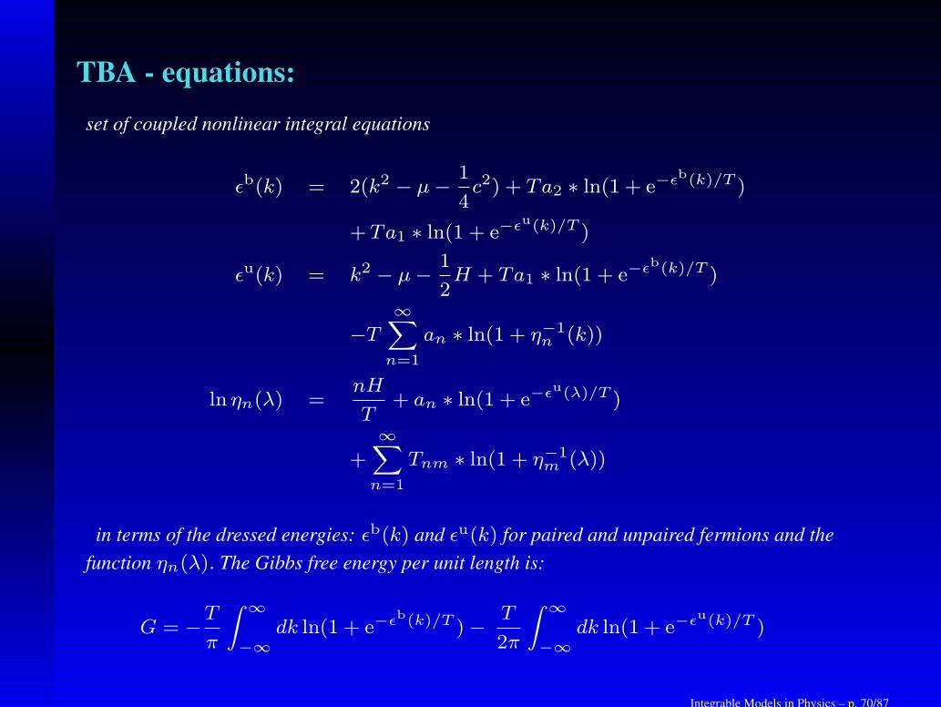
TBA - equations:
set of coupled nonlinear integral equations
ǫb(k) = 2(k2 − µ− 1
4c2) + Ta2 ∗ ln(1 + e−ǫb(k)/T )
+Ta1 ∗ ln(1 + e−ǫu(k)/T )
ǫu(k) = k2 − µ− 1
2H + Ta1 ∗ ln(1 + e−ǫb(k)/T )
−T∞∑
n=1
an ∗ ln(1 + η−1n (k))
ln ηn(λ) =nH
T+ an ∗ ln(1 + e−ǫu(λ)/T )
+
∞∑
n=1
Tnm ∗ ln(1 + η−1m (λ))
in terms of the dressed energies: ǫb(k) and ǫu(k) for paired and unpaired fermions and the
function ηn(λ). The Gibbs free energy per unit length is:
G = −Tπ
∫ ∞
−∞dk ln(1 + e−ǫb(k)/T )− T
2π
∫ ∞
−∞dk ln(1 + e−ǫu(k)/T )
Integrable Models in Physics – p. 70/87
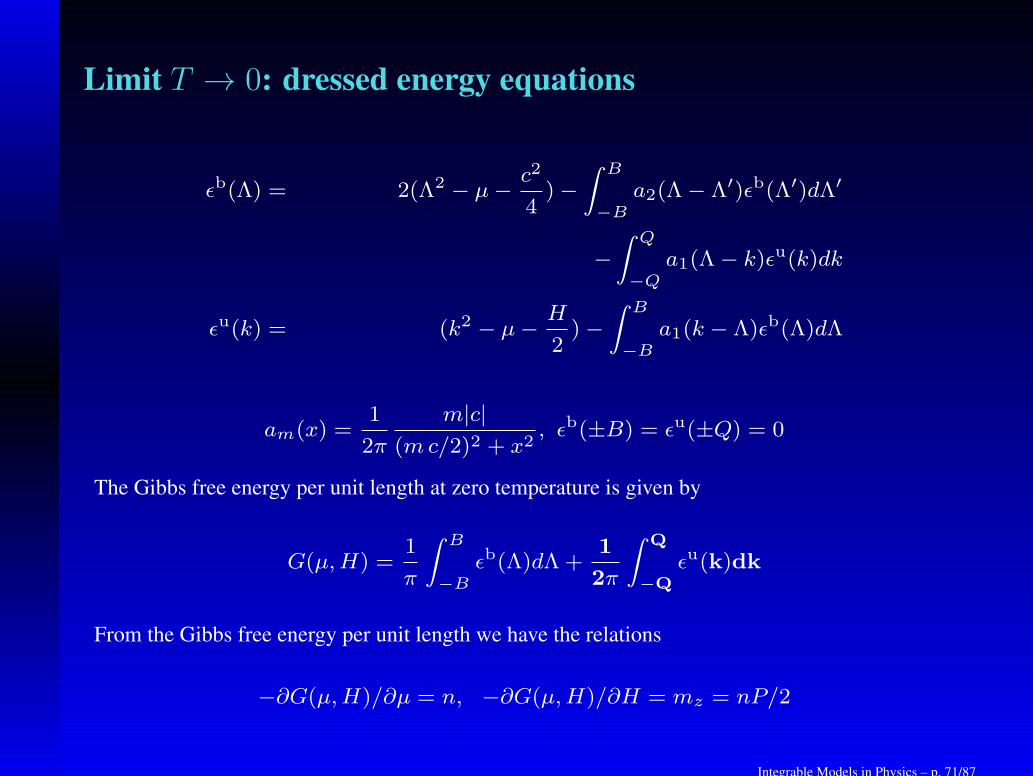
Limit T → 0: dressed energy equations
ǫb(Λ) = 2(Λ2 − µ− c2
4)−
∫ B
−Ba2(Λ− Λ′)ǫb(Λ′)dΛ′
−∫ Q
−Qa1(Λ− k)ǫu(k)dk
ǫu(k) = (k2 − µ− H
2)−
∫ B
−Ba1(k − Λ)ǫb(Λ)dΛ
am(x) =1
2π
m|c|(mc/2)2 + x2
, ǫb(±B) = ǫu(±Q) = 0
The Gibbs free energy per unit length at zero temperature is given by
G(µ,H) =1
π
∫ B
−Bǫb(Λ)dΛ +
1
2π
∫ Q
−Q
ǫu(k)dk
From the Gibbs free energy per unit length we have the relations
−∂G(µ,H)/∂µ = n, −∂G(µ,H)/∂H = mz = nP/2
Integrable Models in Physics – p. 71/87
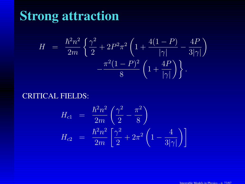
Strong attraction
H =~2n2
2m
{
γ2
2+ 2P 2π2
(
1 +4(1− P )
|γ| − 4P
3|γ|
)
−π2(1− P )2
8
(
1 +4P
|γ|
)}
.
CRITICAL FIELDS:
Hc1 =~2n2
2m
(
γ2
2− π2
8
)
Hc2 =~2n2
2m
[
γ2
2+ 2π2
(
1− 4
3|γ|
)]
Integrable Models in Physics – p. 72/87
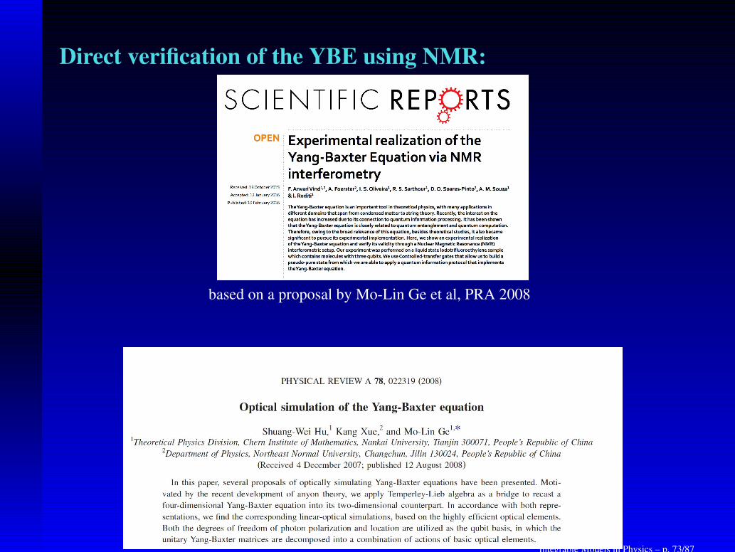
Direct verification of the YBE using NMR:
based on a proposal by Mo-Lin Ge et al, PRA 2008
Integrable Models in Physics – p. 73/87
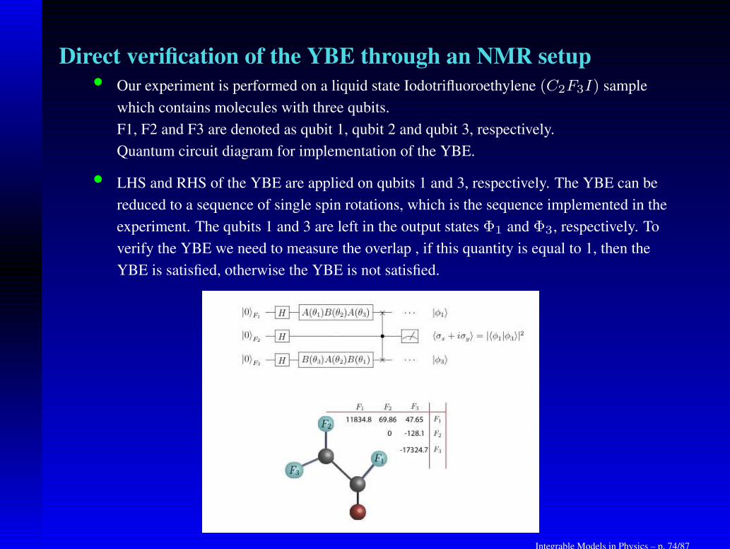
Direct verification of the YBE through an NMR setup• Our experiment is performed on a liquid state Iodotrifluoroethylene (C2F3I) sample
which contains molecules with three qubits.
F1, F2 and F3 are denoted as qubit 1, qubit 2 and qubit 3, respectively.
Quantum circuit diagram for implementation of the YBE.
• LHS and RHS of the YBE are applied on qubits 1 and 3, respectively. The YBE can be
reduced to a sequence of single spin rotations, which is the sequence implemented in the
experiment. The qubits 1 and 3 are left in the output states Φ1 and Φ3, respectively. To
verify the YBE we need to measure the overlap , if this quantity is equal to 1, then the
YBE is satisfied, otherwise the YBE is not satisfied.
Integrable Models in Physics – p. 74/87
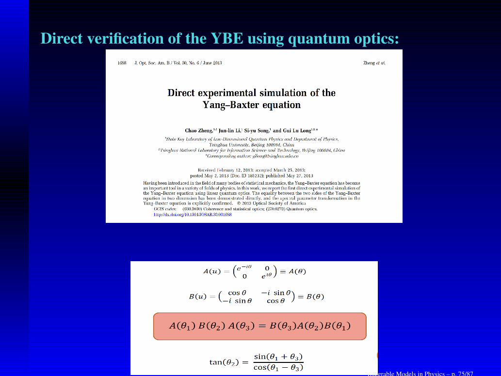
Direct verification of the YBE using quantum optics:
Integrable Models in Physics – p. 75/87
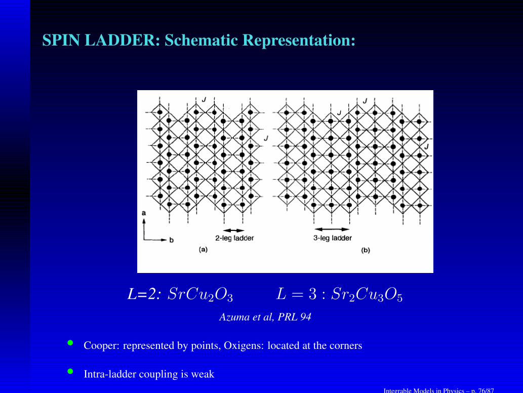
SPIN LADDER: Schematic Representation:
L=2: SrCu2O3 L = 3 : Sr2Cu3O5
Azuma et al, PRL 94
• Cooper: represented by points, Oxigens: located at the corners
• Intra-ladder coupling is weak
Integrable Models in Physics – p. 76/87
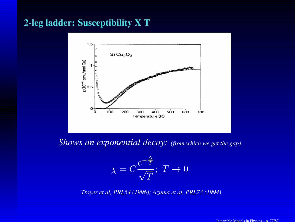
2-leg ladder: Susceptibility X T
Shows an exponential decay: (from which we get the gap)
χ = Ce−
∆T
√T; T → 0
Troyer et al, PRL54 (1996); Azuma et al, PRL73 (1994)
Integrable Models in Physics – p. 77/87
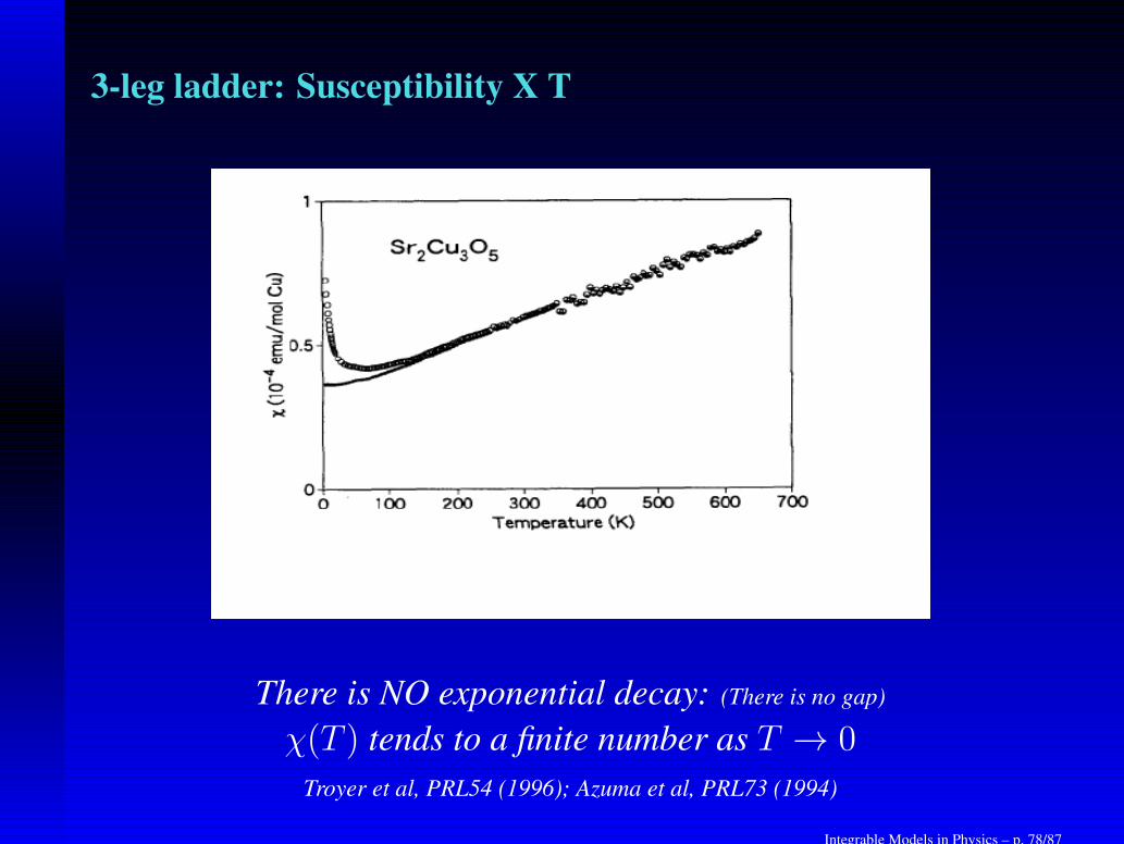
3-leg ladder: Susceptibility X T
There is NO exponential decay: (There is no gap)
χ(T ) tends to a finite number as T → 0
Troyer et al, PRL54 (1996); Azuma et al, PRL73 (1994)
Integrable Models in Physics – p. 78/87
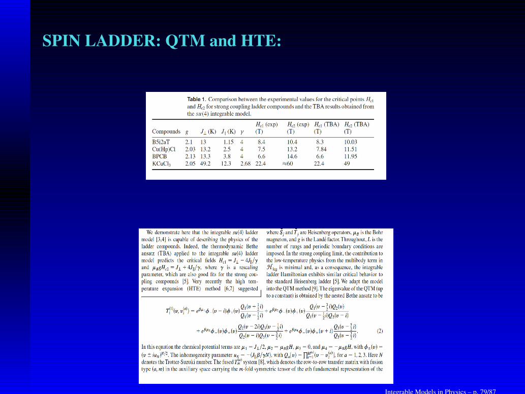
SPIN LADDER: QTM and HTE:
Integrable Models in Physics – p. 79/87
SPIN LADDER: QTM and HTE:
Integrable Models in Physics – p. 80/87
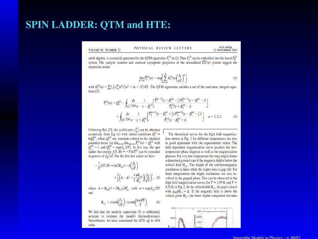
SPIN LADDER: THERMODYNAMICAL PROPERTIES
• The thermal and magnetic properties can be obtained by exact diagonalization or by
analytical methods: the free energy is written in terms of the eigenvalue of the Quantum
Transfer Matrix (QTM) (the QTM eigenvalue satisfies a set on nonlinear eqs. The free
energy can be expanded in powers of J‖/(γT ) up to fifth order, using the High
Temperature Expansion - HTE), and from it we derive the thermodynamical properties by
standard thermodynamics:
• Magnetization
Mz = − ∂
∂Hf(T,H)
• Magnetic susceptibility
χ = − ∂2
∂H2f(T,H)
• Specific heat
c = −T ∂2
∂T 2f(T,H)
Integrable Models in Physics – p. 81/87
LL-Bose gas: the exact solution:• BA- wavefunction:
ψχ (x1, x2, . . . , xN) =∑
P
A(P ) exp(i(kP1x1+· · ·+kPNxN))
A(P ) = Cǫ(P )∏
j<l
(kPj − kPl + ic)
• Energy eigenvalues:
E =~2
2m
N∑
j=1
k2j ,
• BA-equations:
exp(ikjL) = −M∏
ℓ=1
kj − kℓ + i c
kj − kℓ − i cj = 1 . . . N
Integrable Models in Physics – p. 82/87
Geometric Ansatz: the basic idea
• Change to Jacobi coordinates, which allows to remove the
CM-coordinate;
• Change of coordinates to hyperspherical coordinates: radial
component λ and the angular part ~θ = {θ1, θ2, ...θN−2}.
• The relative Hamiltonian now takes the form:
Hrel = − ~2
2µ∇2 +
1
2µω2λ2 + c
∑
j
δ(
dj(~θ))
.
For small λ, Hrel is approximately the one solved by the
Bethe ansatz. For large λ the behaviour is dominated by
that of a harmonic oscillator.
Integrable Models in Physics – p. 83/87
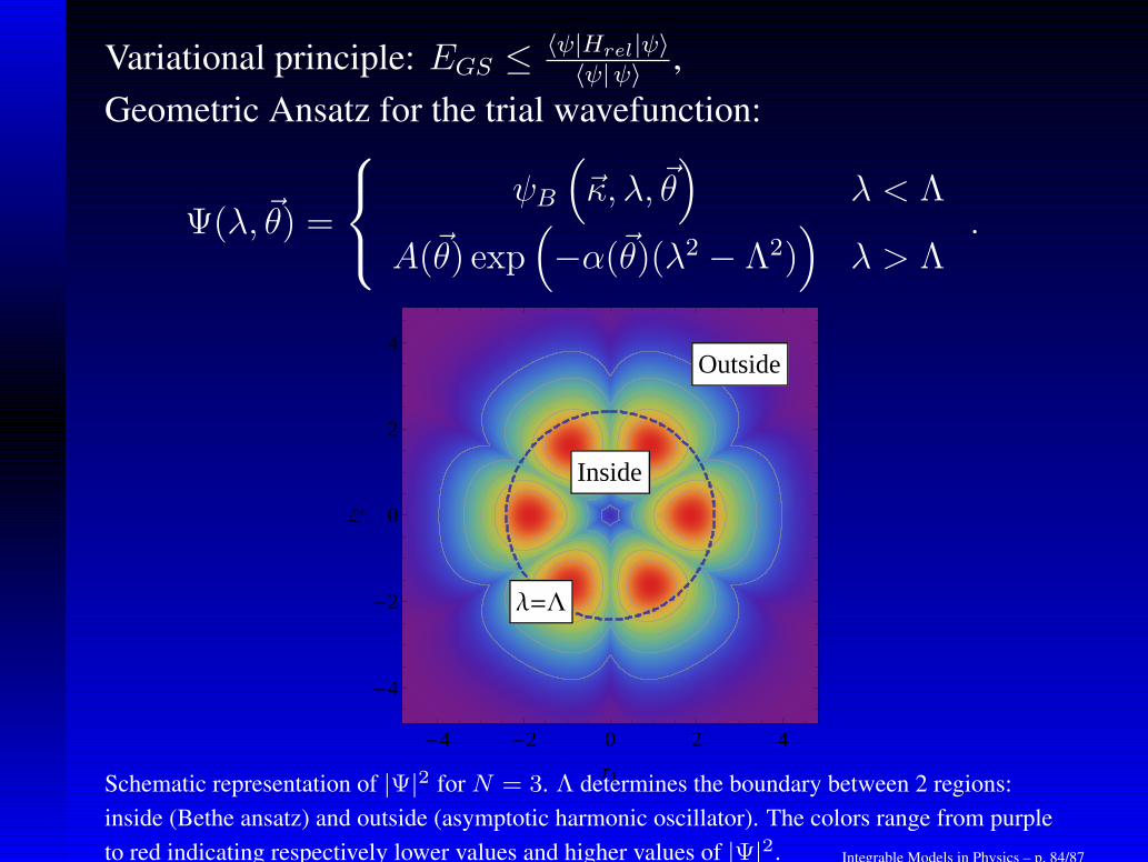
Variational principle: EGS ≤ 〈ψ|Hrel|ψ〉〈ψ|ψ〉 ,
Geometric Ansatz for the trial wavefunction:
Ψ(λ, ~θ) =
ψB
(
~κ, λ, ~θ)
λ < Λ
A(~θ) exp(
−α(~θ)(λ2 − Λ2))
λ > Λ.
-4 -2 0 2 4
-4
-2
0
2
4
r1
r 2
Inside
Outside
Λ=L
Schematic representation of |Ψ|2 for N = 3. Λ determines the boundary between 2 regions:
inside (Bethe ansatz) and outside (asymptotic harmonic oscillator). The colors range from purple
to red indicating respectively lower values and higher values of |Ψ|2. Integrable Models in Physics – p. 84/87
Density ProfilesThe equation of state can be reformulated within the local density
approximation (LDA) by a replacement µ(x) = µ(0)− 12mω2
xx2
in which x is the position and ωx is the trapping frequency, the
total particle number and the polarization are given by:
N
a2xc2
=
∫ ∞
−∞n(x)dx,
P =
∫ ∞
−∞n1(x)dx/(N/(a
2
xc2)).
Integrable Models in Physics – p. 85/87
Universal RatiosIn condensed matter, dimensionless ratios ofquantities that take universal values can providedeep physical insights. Some examples include:
• Wiedemann-Franz ratio
• Sommerfeld-ratio
• Kadowaki-Woods ratio
• Korringa ratio
Why universal ratios are important?
• show that the same particles are responsible for
the two different quantities that form the ratio;
• provide significant constraints on theories;
• demonstrate universality.Integrable Models in Physics – p. 86/87
Wilson Ratio• Dimensionless ratios of quantities that take universal values
can provide deep physical insights.
• The Wilson ratio is defined as the ratio of the magnetic
susceptibility χ to specific heat cv divided by temperature.
• The Wilson ratio has recently been measured in a spin
1/2-ladder compound (C7H10N)2CuBr2.
• Procedure: The main ingredients χ and cv are obtained
from the TBA-equations.
Integrable Models in Physics – p. 87/87


![Integrable Spin Chain of M U N Chern-Simons Theory · arXiv:0808.0170v4 [hep-th] 22 Dec 2008 SNUST 080801 Integrable Spin Chain of Superconformal U(M)×U(N)Chern-Simons Theory Dongsu](https://static.fdocuments.us/doc/165x107/5f6e0974d5ede40ac408ebfc/integrable-spin-chain-of-m-u-n-chern-simons-theory-arxiv08080170v4-hep-th-22.jpg)


