Int J Advanced Design and Manufacturing Technology, Vol. 8...

Int J Advanced Design and Manufacturing Technology, Vol. 8/ No. 1/ March - 2015 13

© 2015 IAU, Majlesi Branch

Statistical Analysis and

Optimization of Factors

Affecting the Spring-back

Phenomenon in UVaSPIF

Process Using Response

Surface Methodology M. Vahdati* & R. A. Mahdavinejad Department of Mechanical Engineering,

University of Tehran, Iran

E-mail: [email protected], [email protected]

*Corresponding author

S. Amini Department of Mechanical Engineering,

University of Kashan, Iran

E-mail: [email protected]

Received: 1 September 2014, Revised: 4 December 2014, Accepted: 6 December 2014

Abstract: Ultrasonic Vibration assisted Single Point Incremental Forming (UVaSPIF) process is an attractive and adaptive method in which a sheet metal is gradually and locally formed by a vibrating hemispherical-head tool. The ultrasonic excitation of forming tool reduces the average of vertical component of forming force and spring-back rate of the formed sample. The spring-back phenomenon is one of the most important geometrical errors in SPIF process, which appear in the formed sample after the process execution. In the present article, a statistical analysis and optimization of effective factors on this phenomenon is performed in the UVaSPIF process based on DOE (Design of Experiments) principles. For this purpose, RSM (Response Surface Methodology) is selected as the experiment design technique. The controllable factors such as vertical step size, sheet thickness, tool diameter, wall inclination angle, and feed rate is specified as input variables of the process. The obtained results from ANOVA (Analysis of Variance) and regression analysis of experimental data, confirm the accuracy of mathematical model. Furthermore, it is shown that the linear, quadratic, and interactional terms of the variables are effective on the spring-back phenomenon. To optimize the spring-back phenomenon, the finest conditions of the experiment are determined using desirability method, and statistical optimization is subsequently verified by conducting the confirmation test.

Keywords: RSM, Single Point Incremental Forming, Spring-back, Ultrasonic Vibration

Reference: Vahdati, M., Mahdavinejad, R. A. and Amini, S., “Statistical Analysis and Optimization of Factors Affecting the Spring-back Phenomenon in UVaSPIF Process Using Response Surface Methodology”, Int J of Advanced Design and Manufacturing Technology, Vol. 8/No. 1, 2015, pp. 13-23.

Biographical notes: M. Vahdati is PhD candidate of mechanical engineering. His current research focuses on incremental sheet metal forming processes. R. A. Mahdavinejad is associated professor of mechanical engineering. His research interest is in traditional and non-traditional processes. S. Amini is assistant professor of mechanical engineering. His research interest includes ultrasonic and machining processes.

14 Int J Advanced Design and Manufacturing Technology, Vol. 8/ No. 1/ March– 2015


1 INTRODUCTION

Nowadays, production industries need to use

economical and flexible processes to enable them to

meet the market demands in a competitive environment

with a minimum cost and time. Thus, researchers have

considered the investigation of operational methods in

order to produce the primary sample and develop new

products. Single Point Incremental Forming (SPIF)

process has been introduced as an attractive and

adaptive method among the rapid prototyping processes

with a high potential to be produced in a small volume.

This process was patented by Leszak in 1967 and its

feasibility was confirmed by Kitazawa et al., in

manufacturing of rotational symmetric parts [1], [2]. In

this process, simple forming tool with hemispherical-

head travels on a sheet metal in a predefined path and

apply local and controllable plastic deformation to

create the final geometry [3-6]. On the other hand, the

geometrical and dimensional accuracy of the SPIF

products is incomplete. In fact, the sheet metal is

clamped simply and can be bended freely during the

process. Thus, when the tool pressure is removed from

the sheet, three different types of error will be detected

on the final geometry (Fig. 1).

Fig. 1 Different types of error on the final geometry in

SPIF process

(1) Sheet bending: This error occurs near the major

base of the part and usually can be removed by

employing backing plate, which lead to the increase of

sheet rigidity.

(2) Lift up: In this state, the formed sheet leaps upward

and the final depth of the part is less than the applied

depth. This geometrical error is recognized as spring-

back.

(3) Pillow effect: This error occurs in the minor base of

the part and appears in the form of the concaved curve,

which result from the undeformed material.

Micari et al., presented some strategies for reduction of

geometrical and dimensional errors involved in the

SPIF process [7]. They discussed on the new trends in

this direction and showed that between different

suggested approaches, the ones based on the use of

optimized tool trajectories seem to be the most

promising. Ambrogio et al., focused on the evaluation

and compensation of elastic spring-back [8]. In this

way, an integrated numerical/experimental procedure

was proposed in order to minimize the shape defects

between the obtained geometry and the desired one.

They have shown that the dimensional accuracy of the

formed sample depends on the tool diameter and

vertical step size. In addition, design of optimized

trajectories was introduced as one of the most

promising way in order to assess the profiles that are

more precise.

Allwood et al., have reported that the sheet metal

forming processes meet typically the geometrical

tolerances in 0.2mm limit, whereas the tolerance

performance of incremental forming processes, are ten

times worse than this situation [9]. The weakness of

geometrical accuracy in incremental forming process in

comparison with CNC machining process is due to the

fact that the sheet metal deformation is not defined

solely by the tool path. Hence, a significant

deformation is created at the outer limits of the contact

zone. Ambrogio et al., performed several tests based on

DOE techniques to fully understand the spring-back

phenomenon with respect to other geometrical

parameters such as wall inclination angle, final depth of

the product and sheet thickness [10]. Subsequently,

they extracted an analytical model to estimate the

“over-deformation” to be applied in order to reduce the

geometrical error.

Meier et al., have shown that the use of Robot in

incremental forming process (Roboforming) has a high

capability to enhance the geometrical accuracy [11].

They suggested two approaches (a model-based and a

sensor-based approach) to determine the geometrical

deviations. For both approaches, one universal

compensation strategy can be used to reduce the

determined deviations in Roboforming. Allwood et al.,

proposed the employment of partially cut-out blanks in

incremental forming [12]. The use of this type of blank

creates a localized deformation earlier, and as a result

reduces the difference between a part made by a

“contour tool path” and the target product geometry.

The influence of these partial cut-outs was evaluated by

forming a simple and a complex part, with and without

cut-outs and with and without backing plates.

The results indicated that partially cut-out blanks lead

to slightly more accurate forming than conventional

blanks when unsupported, but that the accuracy

improvement is less than that which is achieved by use

of a stiff cut-out supporting plate. Therefore, it seems

that the use of partially cut-out blanks does not give a

useful benefit in incremental forming. Review of the

previous researches shows that different approaches



have been made by scientists to increase the

geometrical and dimensional accuracy of the formed

sample. Tool path optimization, process parameters

optimization and development of new methods are

some of these strategies. On the other hand, the

application of ultrasonic vibration in metal forming has

been discussed for many years [13-15]. The

experiments on superimposing the ultrasonic

oscillations on the forming process indicated some

benefits such as reduction of the forming forces,

reduction of the flow stress, reduction of the friction

between die and workpiece and production of the better

surface qualities and higher precision.

Vahdati et al. [16], [17] showed that the ultrasonic

excitation of hemispherical-head tool in SPIF process

(UVaSPIF), reduces the average of vertical component

of forming force and spring-back rate of the formed

sample. Thus, the sheet metal will be formed

incrementally in the presence of ultrasonic vibration

with given frequency and specified amplitude as

compared to the previous researches. Hence, in the

present article, the analysis and optimization of spring-

back phenomenon in UVaSPIF process is done based

on DOE principles using RSM technique. The

objectives of this research unfold on extraction of

regression model and mathematical equation resulting

from ANOVA for spring-back coefficient and access to

optimal conditions of the experiment.

2 METHODOLOGY OF STATISTICAL ANALYSIS

A model presented in Fig. 2 can introduce the process

under study. With the assumption of independency of

controllable factors ( iX ) and response of the process

( iY ), the goal is to obtain the mathematical relation

between the output variable and the input variables

with a minimum error.

Fig. 2 General model of the process

For this purpose, the methodology of statistical analysis

in this research includes the following seven steps:

(1): Selecting the response variable

(2): Selecting the controllable factors

(3): Selecting the experiment design

(4): Experiment execution

(5): Measuring the response variable

(6): Data analysis

(7): Optimization and confirmation

2.1. Selecting the response variable

For evaluation of the spring-back rate, a criterion

namely spring-back coefficient ( K ) is used which can

be calculated from the following relation [18]:

01

0.

2

2ave

th

Kt

h

(1)

In this relation, 1h is the applied depth on the sample

geometry; 0t is the initial thickness of the sheet, and

.aveh is the average of the measured depth after

unclamping the formed sample. With regard to the

above relation, to the extent that the K parameter

becomes closer to the number one ( 1K ), to the

same extent, it denotes the reduction of spring-back

rate. Hence, in this research, the spring-back coefficient

is considered as the response variable.

2.2. Selecting the controllable factors The ultrasonic generator and transducer are the

components of production and transmission of

vibration in this process, respectively [16], [17]. With

regard to the fact that during the process execution, the

applied force on the forming tool will cause a change in

the vibration conditions of the tool, so that the vibration

parameters of the process such as generator power,

frequency, and amplitude of vibration are considered as

the uncontrollable input factors. Thus, five controllable

factors of vertical step size ( ), sheet thickness ( t ),

tool diameter ( d ), wall inclination angle ( ) and feed

rate ( f ) were selected as the input variables of the

experiment and each of them were studied at three

levels of low (-1), central (0) and high (+1). The high

and low levels of each parameter are coded by +1 and -

1. In addition, the coded value of each desirable middle

level is calculated through the following relation [19]:

max min

max min

2 ( )

( )

x x xX

x x

(2)

In this relation, X is the coded value of concerned

parameter with the actual value of x (between minx

and maxx ). minx and maxx have the actual low and high

values of the parameter accordingly. Table 1 shows the

input variables and experimental design levels used

with coded and actual values. The variation range of

these factors was determined based on the primary



experiments, which lead to safe production of the final

geometry.

Table 1 Input variables with design levels

Variable Notation Unit -1 0 +1

Vertical

step size mm 0.25 0.5 0.75

Sheet

thickness t mm 0.4 0.7 1

Tool

diameter d mm 10 15 20

Wall

inclination

angle

40 50 60

Feed rate f mm/min 1500 2000 2500

2.3. Selecting the experiment design

In the present research, RSM is used as the experiment

design technique. In this method, there is a set of

mathematical and statistical techniques, which are

useful for modeling, and analysis of the problems [20],

[21]. In such problems, the relation between response

and input variables is unknown. Thus, the first step in

this method is to find a suitable approximation of the

real relation existing between the response variable

( y ) and the set of input variables ( x ). The

approximating functions are in the form of the linear

and quadratic models and are written in the form of the

following relations:

0 1 1 2 2 ... k ky x x x (3)

2

0

1 1

k k

i i ii i ij i j

i i i j

y x x x x

(4)

In the above functions, 0 is the constant value, i is

the first-order (linear) coefficient, ii is the second-

order (quadratic) coefficient, ij is the interaction

coefficient, k is the number of independent variables,

and is the rate of error. In this research, the second-

order model and Box-Behnken Design (BBD) are used.

The software used for experiment design and statistical

analysis is Minitab [22]. Table 2 shows the design

matrix with 46 tests in the form of coded runs. Five

tests are repeated at the central levels of parameters

(zero level).

Table 2 Design matrix with measured and calculated results Test

no. t d f .( )aveh mm K

1 0 0 -1 +1 0 29.629 1.01238

2 0 0 +1 -1 0 29.602 1.01329

3 0 0 -1 0 +1 29.635 1.01217

4 0 +1 -1 0 0 29.869 1.00431

5 0 0 0 0 0 29.612 1.01295

6 0 0 0 0 0 29.612 1.01295

7 -1 0 -1 0 0 29.871 1.00427

8 0 0 0 +1 -1 29.609 1.01305

9 0 +1 0 -1 0 29.824 1.0058

10 -1 0 0 0 -1 29.827 1.00573

11 0 0 0 0 0 29.612 1.01295

12 0 +1 0 0 -1 29.821 1.0059

13 -1 -1 0 0 0 29.767 1.00778

14 0 -1 0 -1 0 29.584 1.01397

15 0 0 -1 -1 0 29.818 1.00603

16 +1 0 0 0 -1 29.557 1.01481

17 0 0 0 -1 -1 29.615 1.01285

18 0 0 0 +1 +1 29.606 1.01315

19 0 0 -1 0 -1 29.815 1.00613

20 0 -1 0 +1 0 29.566 1.01458

21 0 -1 -1 0 0 29.623 1.01264

22 +1 0 +1 0 0 29.55 1.01505

23 0 0 +1 +1 0 29.59 1.01369

24 0 0 0 0 0 29.612 1.01295

25 0 -1 +1 0 0 29.563 1.01468

26 0 +1 0 0 +1 29.687 1.01037

27 +1 0 0 0 +1 29.555 1.01488

28 +1 0 -1 0 0 29.617 1.01278

29 +1 0 0 +1 0 29.553 1.01495

30 -1 0 0 -1 0 29.83 1.00563

31 0 0 0 0 0 29.612 1.01295

32 0 +1 0 +1 0 29.682 1.01054

33 +1 0 0 -1 0 29.559 1.01474

34 0 0 0 -1 +1 29.614 1.01288

35 +1 +1 0 0 0 29.672 1.01087

36 -1 +1 0 0 0 29.873 1.00418

37 0 +1 +1 0 0 29.677 1.0107

38 0 -1 0 0 +1 29.572 1.01438

39 0 0 +1 0 +1 29.594 1.01356

40 -1 0 +1 0 0 29.771 1.0076

41 +1 -1 0 0 0 29.545 1.0153

42 -1 0 0 +1 0 29.775 1.00747

43 0 -1 0 0 -1 29.578 1.01417

44 0 0 +1 0 -1 29.598 1.01342

45 -1 0 0 0 +1 29.779 1.00734

46 0 0 0 0 0 29.612 1.01295



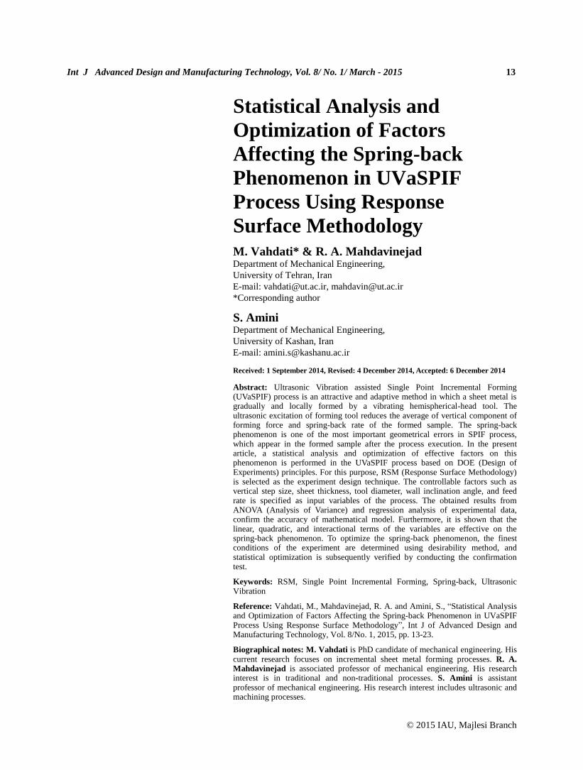
2.4. Experiment execution

The sheet metal is Al 1050-O, which is used in

annealed form (350°c for 2 hours). The hydraulic oil

(HLP68) was used as lubricator [23]. The

hemispherical-head tools were designed and

manufactured in three diameters of 10, 15, and 20mm

(Fig. 3) in accordance with the instruction of design,

manufacturing, and test of vibrating forming tools [16].

For imposing the ultrasonic vibration on the forming

tools, an ultrasonic generator with power of 1000 watt and operational frequency of 20 kHz were used. The

amplitude of vibration of forming tools was measured

to be 7.5 microns. The circular speed of forming tools

was adjusted in 125rpm. Figure 4 shows the fixture

components in SPIF process. The sheet metal is placed

between clamping plate and backing plate. The sample

geometry was considered in the form of pyramid

frustum with the base dimension of 80×80mm and

depth of 30mm (Fig. 5).

Fig. 3 Forming tools

Fig. 4 Components of the fixture in SPIF process

Fig. 5 Dimensional characteristics of the formed sample

Tool path strategy is in the form of the gradual

imposing of wall inclination angle (based on successive

horizontal-vertical steps in one face of sample

geometry) and then the linear motion in the working

plane (Fig. 6). Figure 7 shows the simulation of tool

path strategy in Cimco software for the wall inclination

angle of 60 [24]. The tests were performed in

accordance with the 46 runs included in the Table 2.

The samples were formed in accordance with the

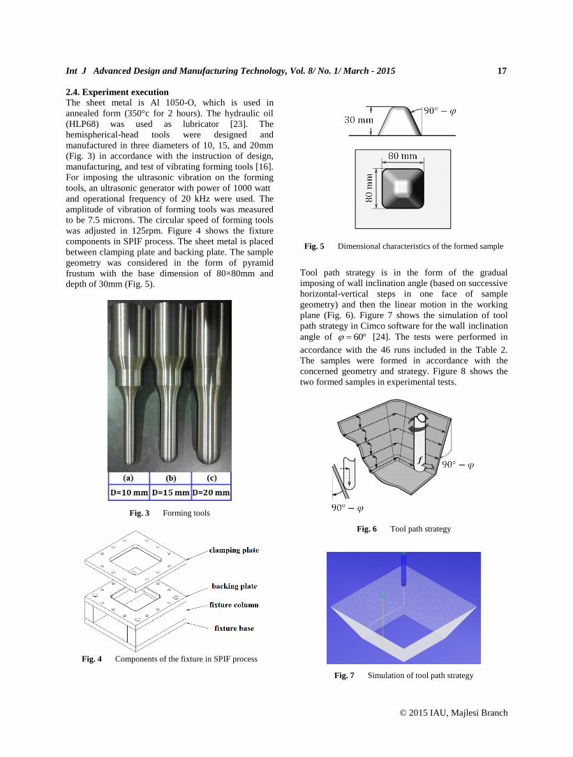
concerned geometry and strategy. Figure 8 shows the

two formed samples in experimental tests.

Fig. 6 Tool path strategy

Fig. 7 Simulation of tool path strategy



(a) Test no. = 43

(b) Test no. = 9

Fig. 8 Two formed samples in the experimental tests

2.5. Measuring the response variable

The depth of formed samples was measured in the

position of spring-back creation by the Contourgraph

system and its average was registered as the .aveh (Fig.

9). Table 2 shows the results of measuring ( .aveh ) and

calculation of the spring-back coefficient ( K ) of the

formed samples.

2.6. Data analysis

Analysis of experimental data is performed by

ANOVA, which is a powerful tool to study the

importance of a parameter and identify the significance

of its effect. In addition, in order to create the

mathematical functions between the response variable

and the effective parameters, the regression analysis is

employed [19]. Confidence level ( ) is considered as

equal to 0.05 and statistically, it means that the final

model can predict the data with an error less than 5%.

The effectiveness of a term is specified through

“ P value ”, related to the corresponding term. Thus,

the terms are identified with the “ P value ”, as

significant and with the “ P value ”, as

insignificant. To the extent that the “ P value ” related

to a term is smaller, to the same extent the significance

of that term in the model is greater. Thus, with the

assumption of 0.05 and based on the primary

obtained results from ANOVA, the first-order

parameters: vertical step size ( ), sheet thickness ( t ),

tool diameter ( d ), wall inclination angle ( ) and feed

rate ( f ), the second-order terms: 2 ,

2t , 2d and

interactional terms: td , t , tf , d and df were

determined as the effective terms on the spring-back

coefficient and the other terms as the ineffective terms.

(a) Plunger motion on the sample surface

(b) Difference between the imposed and measured depth

Fig. 9 Measuring the depth of formed sample

In the final step of data analysis, the terms with inactive

effects should be removed from the model and just the

terms with active effects to be analyzed. Thus, all

ineffective terms with the “ 0.05P value ” are

deleted from the analysis and all terms with the

“ 0.05P value ” in the final step of ANOVA will be

present. Table 3 shows the regression table, which is

the result from the final ANOVA, based on the

effective terms.

As it is observed, all terms existing in Table 3 have

appeared with the “ 0.05P value ”, and as effective

terms on the response variable. The emergence of

positive sign (+) for regression coefficients, states the

presence of a direct relation between the terms and

response variable. Whereas, the emergence of negative

sign (-) for regression coefficients shows the presence

of a reverse relation between the terms and response

variable. In the continuation, the role of the effective

parameters for achieving an ideal situation of the

response variable will be studied. Thus, the reduction

of spring-back coefficient ( K ) is determined as the

ideal situation.



Table 3 Regression table based on the effective terms

Term Regression coefficient T-value P-

value

Constant 1.01273 4588.851 0

0.00396 19.188 0

t -0.0028 -13.572 0

d 0.00195 9.47 0

0.00091 4.426 0

f 0.00079 3.836 0.001

-0.0019 -7.244 0

t t -0.00134 -5.09 0

d d -0.00113 -4.288 0

t d 0.00109 2.634 0.013

t 0.00103 2.501 0.018

t f 0.00106 2.579 0.015

d -0.00149 -3.603 0.001

d f -0.00148 -3.572 0.001

2 96.13 %R 2 94.56 %adjustedR

The following relation expresses the regression

equation of spring-back coefficient as a function of the

coded effective values:

(5)

2

2 2

1.01273 0.00396 0.0028 0.00195

0.00091 0.00079 0.0019

0.00134 0.00113 0.00109

0.00103 0.00106 0.00149

0.00148

K t d

f v

t d td

t tf d

df

The investigation of the T-value belonging to the

effective terms shows that:

(1): Vertical step size ( ) as the linear effect has the

greatest effect and the product of sheet thickness and

wall inclination angle ( t ) as the interactional effect,

has the least effect on the spring-back coefficient. In

other words, the effect of is 7.6 times of the t

effect.

(2): Vertical step size ( ) among the linear effects has

the greatest effect on the spring-back coefficient.

(3): Vertical step size ( ) among the quadratic effects

(2 ) has the greatest effect on the spring-back

coefficient.

(4): The product of tool diameter and wall inclination

angle ( d ) and the product of tool diameter and feed

rate (df ) among the interactional effects have the

greatest effect on the spring-back coefficient.

As it is observed in Table 3, the correlation coefficients

of 2R and 2

.adjR show the peak values of 96% and 94%

respectively. As a result, a high correlation is

established between the observed data in the

experimental tests and the predicted responses resulting

from the regression equation. Hence, the ability of the

fitted model and accuracy of the regression equation in

describing and predicting the changes of the response

variable are confirmed. Table 4 shows the obtained

results from the ANOVA.

Table 4 ANOVA results for the final model

Source of variation Degree of freedom F-value P-

value

Regression 13 61.21 0

Linear 5 135.28 0

1 368.19 0

t 1 184.21 0

d 1 89.68 0

1 19.59 0

f 1 14.71 0.001

Square 3 24.58 0

1 52.48 0

t t 1 25.91 0

d d 1 18.38 0

Interaction 5 9.12 0

t d 1 6.94 0.013

t 1 6.25 0.018

t f 1 6.65 0.015

d 1 12.98 0.001

d f 1 12.76 0.001

Residual Error 32 - -

Lack of Fit 27 1.432 0.093

Pure Error 5 - -

Total 45 - -

In order to investigate the accuracy of the regression

model, in addition to 2R evaluation, the Lack of Fit

(LOF) test is also used. The significance of this test

( 0.05LOFP value ) indicates that the data are not

well placed around the model and it is not possible to

use the model to predict the response variable. Thus,

with the confirmation of the insignificance of the LOF

test ( 0.05LOFP value ), it is possible to find out that

the model can be well fitted on the data. As it is

observed in the Table 4, LOF test for the response

variable is not significant and consequently, the

presented model shows the data trends well. On the



other hand, the best analysis is performed when the

regression is effective and the LOF is ineffective

concurrently [19]. Thus, with regard to the P value ,

it is observed that the regression term, is effective and

the LOF term is ineffective.

The plot of normal probability is a useful means to

check the accuracy of normal distribution of the

residuals. The residual is defined in the form of the

difference between the measured response in the

experimental test and the predicted response by the

final model. The obtained results from this research

show that the residuals in this plot generally follow a

straight line and there is no evidence on abnormality,

asymmetry, and divergence (Fig. 10). Also, it is

possible to investigate the model competency by

studying the behavior of the residuals. If the regression

model is appropriate, subsequently the residuals have

no structure. As it is shown in Fig. 11, the residuals

have been distributed randomly around the zero axis

and the diagram does not include any specific pattern,

hence the final model is reliable and suitable.

Fig. 10 Normal probability plot

Fig. 11 Residual plot

The response behavior can be shown in terms of input

variables in the form of 3D diagrams (surface plot) and

2D diagrams (contour plot). In these diagrams, the

interactional effects of the two input variables on the

response variable are observable and the values of other

input variables are considered fixed at the central levels

(zero level). The relationship of the spring-back

coefficient with vertical step size ( ) and tool diameter

(d ) has been shown in Fig. 12. As it is observed, the

reduction of tool diameter ( d ) causes the reduction of

spring-back coefficient and this effect is intensified

with the reduction of vertical step size ( ).

(a) Surface plot

(b) Contour plot

Fig. 12 Relationship of the spring-back coefficient ( K )

with vertical step size ( ) and tool diameter ( d )

On the other hand, the increase of sheet thickness ( t )

along with the reduction of wall inclination angle ( ),

causes the reduction of spring-back coefficient (Fig.

13).

2.7. Optimization and confirmation

In this research, desirability method was used as the

optimization technique with regard to the simplicity,

flexibility, and accessibility in the software. Drringer

and Suich introduced this method in 1980 [25]. In this

technique, first the output response of iy is converted

into dimensionless desirability of id ( 0 1id ), such

that the higher value of id signifies the greater

desirability of iy and if the response is outside the

acceptable limit, 0id .



(a) Surface plot

(b) Contour plot

Fig. 13 Relationship of the spring-back coefficient ( K )

with sheet thickness ( t ) and wall inclination angle ( )

Thus, for the output response, a separate desirability

function with a range of 0 to 1 is obtained. In this

research, the goal of the desirability function is the

minimization of the response variable (reduction of

spring-back coefficient), where the desirability is

defined in the following form:

(6)

1

0

r

y L

U yd L y U

U L

y U

In the above relation, L and U are the low and high

limits of y , respectively. The shape of desirability

function depends on the weight field (r) which is used

to express the degree of significance of the target value.

Here, the weight value is assumed equal to one ( 1r )

and consequently, the desirability function is defined in

a linear mode. Table 5 shows the specifications of the

desirability function for the output response.

Table 5 Specifications of the desirability function

Output

response

Desirability

function

Function

target

Weight

value (r)

y K ( )d y 1K 1

Figure 14 shows the diagrams of the spring-back

coefficient model which is the resultant of the

optimization process at the optimal point. As it is

observed, the vertical line in red color shows the

optimal values of input variables and the horizontal line

in blue color shows the optimal value of output

response. Thus, the effect of the input variables to

achieve the target of function is identifiable and

interpretable from diagram simply.

Fig. 14 Behavior of the spring-back coefficient ( K ) at the

optimal points of input parameters

Table 6 Optimal values of the input variables

Input

variable

Coded optimal

value

Actual optimal

value

-1 0.25 mm

t 0.7071 0.91 mm

d -1 10 mm

0.8384 58.38⁰

f -1 1500 mm/min

Table 6 shows the optimal values of the input variables

to achieve the desirability function target. Therefore,

the reduction of vertical step size ( ), tool diameter

(d ) and feed rate ( f ) along with the increase of sheet

thickness ( t ) and wall inclination angle ( ) leads to

the reduction of spring-back coefficient. As it is

observed, the optimal angle of wall inclination ( ) was

determined to be 58.38°. Also, the optimal value of

output response, which results from the regression

equation is equal to one (1) and the value of the

corresponding desirability function with it, is equal to

0.9971. Hence, with regard to the high value of

separate desirability function, it can be realized that the

procedure of process optimization has well fulfilled a

pre-determined target successfully.

In order to confirm the optimized response and to

measure the accuracy of the presented model, the

experimental test was conducted by the finest



conditions of input variables. Table 7 shows the input

variables of the test and Fig. 15 shows the formed

sample after performing the confirmation test. Table 8

presents the obtained results from the confirmation test

and its comparison with the optimized result.

Table 7 Input variables of the confirmation test

variable value 0.25 mm

t 0.9 mm

d 10 mm

58⁰

f 1500 mm/min

(a) 3D view

(b) Front view

Fig. 15 Formed sample in the confirmation test

Table 8 Comparison between the obtained results from confirmation

test and optimization process

K (confirmation test)

K (optimization process)

Difference percent

1.00512 1 0.51 %

This comparison shows that the error of regression

model to predict the spring-back coefficient is less than

1%. Thus, the accuracy of regression model to predict

the response variable is confirmed.

3 CONCLUSION

In this article, analysis and optimization of the spring-

back phenomenon in the UVaSPIF process was

conducted based on DOE principles using RSM

technique. The major accomplishments of this research

are summarized as follows:

The primary achieved results from ANOVA with

the assumption of 0.05 showed that the linear

terms: vertical step size ( ), sheet thickness ( t ),

tool diameter ( d ), wall inclination angle ( ) and

feed rate ( f ), the quadratic terms: 2 , 2t , 2d

and the interactional terms: td , t , tf , d and

df , can have effect on the spring-back

phenomenon.

The regression equation, which results from

ANOVA, was extracted to predict the spring-back

coefficient in UVaSPIF process. The competency

of the final model was investigated by the

correlation coefficients, Lack of Fit (LOF) test,

normal probability plot, and diagram of residuals.

Consequently, the ability of the fitted model and

accuracy of the regression equation in describing

and predicting the behavior of spring-back

coefficient was confirmed.

In this research, with regard to the

comprehensiveness of the presented mathematical

model, a broad range of effective factors on the

spring-back phenomenon is covered. Thus, the

presented model can be utilized in SPIF and TPIF

processes in addition to prediction and control of

spring-back parameters in UVaSPIF process.

The optimal values of input variables were

extracted to access the least spring-back

coefficient. The optimization results indicated that

the reduction of vertical step size, tool diameter,

and feed rate along with the enhancement of sheet

thickness and wall inclination angle, lead to the

reduction of spring-back coefficient. Also, the

optimal angle of wall inclination was determined

to be 58.38°.

The high value of the desirability function

corresponding to the spring-back coefficient

( 0.9971d ), exhibited that the optimization

procedure of the process has successfully fulfilled

a pre-determined target.

A comparison between the achieved results from

the confirmation test and the optimization process

showed that the error of regression model for

prediction of spring-back coefficient is less than

1%. This proves the accuracy of proposed

regression model.

ACKNOWLEDGMENTS

The authors would like to thank Dr. Moradi and Mr.

Hosseinpour for their technical assistance.



REFERENCES

[1] Leszak, E., U.S. Patent Application for a “Apparatus and process for incremental dieless forming”, Docket No. 3342051A, filed 1967.

[2] Kitazawa, K., Wakabayashi, A., Murata, K., and Yaejima, K., “Metal-flow phenomena in computerized numerically controlled incremental stretch-expanding of aluminium sheets”, Journal of Japan Institute of Light Metals, Vol. 46, 1996, pp. 65-70.

[3] Petek, A., Jurisevic, B., Kuzman, K., and Junkar, M., “Comparison of alternative approaches of single point incremental forming processes”, Journal of Materials Processing Technology, Vol. 209, 2009, pp. 1810-1815.

[4] Duflou, J., Tunckol, Y., Szekeres, A., and Vanherck, P., “Experimental study on force measurements for single point incremental forming”, Journal of Materials Processing Technology, Vol. 189, 2007, pp. 65-72.

[5] Jeswiet, J., Micari, F., Hirt, G., Bramley, A., Duflou, J., and Allwood, J., “Asymmetric single point incremental forming of sheet metal”, CIRP Annals - Manufacturing Technology, Vol. 54, No. 2, 2005, pp. 623-649.

[6] Thibaud, S., Ben Hmida, R., Richard, F., and Malécot, P., “A fully parametric toolbox for the simulation of single point incremental sheet forming process: Numerical feasibility and experimental validation”, Simulation Modelling Practice and Theory, Vol. 29, 2012, pp. 32-43.

[7] Micari, F., Ambrogio, G., and Filice, L., “Shape and dimensional accuracy in Single Point Incremental Forming: State of the art and future trends”, Journal of Materials Processing Technology, Vol. 191, 2007, pp. 390-395.

[8] Ambrogio, G., Costantino, I., De Napoli, L., Filice, L., and Muzzupappa, M., “Influence of some relevant process parameters on the dimensional accuracy in incremental forming: a numerical and experimental investigation”, Journal of Materials Processing Technology, Vol. 153C/154C, 2004, pp. 501-507.

[9] Allwood, J. M., King, G. P. F., and Duflou, J., “A structured search for applications of the incremental sheet-forming process by product segmentation”, Proceedings of the Institution of Mechanical Engineers, Part B: Journal of Engineering Manufacture, Vol. 219, No. 2, 2005, pp. 239-244.

[10] Ambrogio, G., Cozza, V., Filice, L., and Micari, F., “An analytical model for improving precision in single point incremental forming”, Journal of Materials Processing Technology, Vol. 191, 2007, pp. 92-95.

[11] Meier, H., Buff, B., Laurischkat, R., and Smukala, V., “Increasing the part accuracy in dieless robot-based incremental sheet metal forming”, CIRP

Annals - Manufacturing Technology, Vol. 58, 2009, pp. 233-238.

[12] Allwood, J. M., Braun, D., and Music, O., “The effect of partially cut-out blanks on geometric accuracy in incremental sheet Forming”, Journal of Materials Processing Technology, Vol. 210, 2010, pp. 1501-1510.

[13] Siegert, K., Ulmer, J., “Superimposing ultrasonic waves on the dies in tube and wire drawing”, Journal of Engineering Materials and Technology, Vol. 123, 2001, pp. 517-523.

[14] Hung, J.-C., Hung, C., “The influence of ultrasonic-vibration on hot upsetting of aluminum alloy”, Ultrasonics, No. 43, 2005, pp. 692-698.

[15] Tolga Bozdana, A., Gindy, N. N. Z., and Li, H., “Deep cold rolling with ultrasonic vibrations – a new mechanical surface enhancement technique”, International Journal of Machine Tools and Manufacture, No. 45, 2005, pp. 713-718.

[16] Vahdati, M., Mahdavinejad, R. A., Amini, S., Abdullah, A., and Abrinia, K., “Design and manufacture of vibratory forming tool to develop “ultrasonic vibration assisted incremental sheet metal forming” process”, Modares Mechanical Engineering, Vol. 14, No. 11, 2014, pp. 68-76 (In Persian).

[17] Vahdati, M., Mahdavinejad, R. A., and Amini, S., “Investigation of the Ultrasonic Vibration Effect in Incremental Sheet Metal Forming (ISMF) Process”, Proceedings of the Institution of Mechanical Engineers, Part B: Journal of Engineering Manufacture, (to be published).

[18] Vahdati, M., Sedighi, M., and Khoshkish, H., “An analytical model to reduce spring back in Incremental Sheet Metal Forming (ISMF) process”, International Journal of Advanced Materials Research (AMR), Vols. 83-86, 2010, pp. 1113-1120.

[19] Montgomery, D. C., “Design and Analysis of Experiments”, 3rd ed., New York, John Wiley & Sons, 1991.

[20] Khuri, A. I., Cornell, J. A., “Response Surfaces Design and Analysis”, 2nd ed., New York, Marcel Dekker, 1996.

[21] Myers, R. H., Montgomery, D. C., “Response Surface Methodology: Process and Product Optimization Using Designed Experiments”, 2nd ed., New York, John Wiley & Sons, 2002.

[22] Minitab Software Package, Ver. 16, http://www.minitab.com.

[23] DIN 51524, Part 2. [24] CIMCO Software Package, Ver. 5,

http://www.cimco.com. [25] Myers, R. H., Montgomery, D. C., and Anderson-

Cook, C. M., “Response Surface Methodology: Process and Product Optimization Using Designed Experiments”, 3rd ed., New York, John Wiley & Sons, 2009.

http://www.minitab.com/

http://www.cimco.com/

Int J Advanced Design and Manufacturing Technology, Vol. 8...

Documents

Transcript of Int J Advanced Design and Manufacturing Technology, Vol. 8...