Instructions for data analysis software - IUGONET · 2018-11-08 · timespan, ‘yyyy-mm-dd ......
103
Instructions for data analysis software: - Preparation - The IUGONET project and its products for space weather study - Installation - How to Use SPEDAS, part1 - How to Use SPEDAS, part2 Published by IUGONET Project Team, Sep. 2017. http://www.iugonet.org/?lang=en
Transcript of Instructions for data analysis software - IUGONET · 2018-11-08 · timespan, ‘yyyy-mm-dd ......

Instructions for data analysis software:- Preparation- The IUGONET project and its products for space weather study- Installation- How to Use SPEDAS, part1- How to Use SPEDAS, part2
Published by IUGONET Project Team, Sep. 2017. http://www.iugonet.org/?lang=en

IUGONET System: MetaData System for Space Weather and Earth Observation Data Analysis
Shuji AbeInternational Center for Space Weather Science and Education
プレゼンター
プレゼンテーションのノート
Good morning. I am Shuji Abe, from ICSWSE Japan. Today, I will talk the following title
Outline
Today’s Outline:This hands-on have 4 topics
1. Introduction to the IUGONET2. Analysis software(SPEDAS) hands-on 1
loading and plotting built-in databreak
3. Analysis software(SPEDAS) hands-on 2figure reformation and data processing
4. Analysis software(SPEDAS) hands-on 3loading and plotting external data
プレゼンター
プレゼンテーションのノート
Here is a brief outline today. When you prepare figures used for the scientific presentations and papers, data processing and adjustment of details to improve the appearance of the figures are required. You can learn how to process data and adjust figure axis and captions in hands-on 2.
Characteristics of Upper Atmosphere
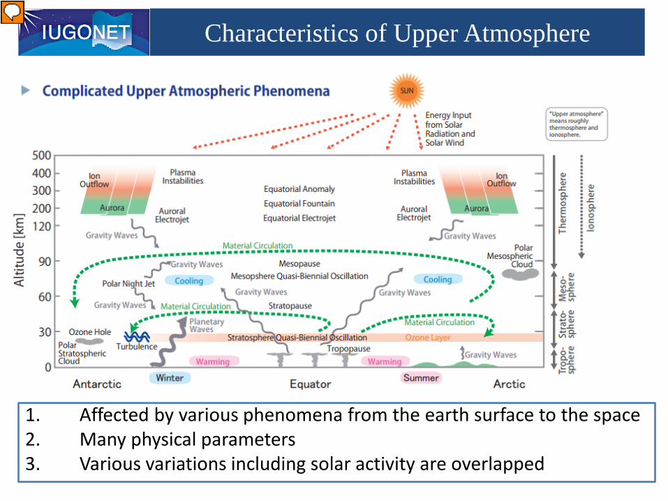
1. Affected by various phenomena from the earth surface to the space2. Many physical parameters3. Various variations including solar activity are overlapped
プレゼンター
プレゼンテーションのノート
This figure shows the complicated upper atmosphere phenomena, the scientific target of IUGONET. Vertical axis shows altitude, horizontal axis shows latitude and Seasons. The features of this region is one, two, and there.
Ground Observations for Upper Atmosphere
JpGU 2014
プレゼンター
プレゼンテーションのノート
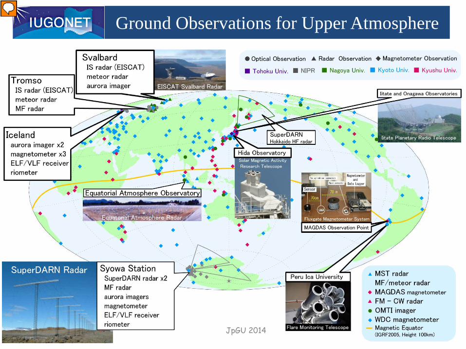
To study the physics of the upper atmosphere, many universities and institutes constructed global ground-based observation networks, which cover from the equator to the north pole and south pole. This map shows the location of the instruments installed by the IUGONET members. There are various kinds of instrument, for example, radar, imager, magnetometer, and so on. That means that we need to analyze various kinds of data.

Objectives of the IUGONET
Observational data should be quality controlled and managed by the specialists
who know the observations. For users….It was not easy to reach a
necessary information, since databases are distributed in various universities and
institutes.
IUGONET provides a new research platform thatenables metadata extracted from ground-basedobservation data to be shared.In addition, IUGONET developed analysissoftware to access and analyze data in anintegrated fashion.
SolutionProblem
プレゼンター
プレゼンテーションのノート
But, we have a problem. The database of each data has been constructed separately by each university, so it is often difficult for researchers to find the data. To solve this issue, IUGONET created metadata of the data and build the database system for handling them. So, now we can get various information of the observational data by using the metadata database.

Overview of the project
7
The Inter-university Upper atmosphere Global Observation NETwork (IUGONET) project aims at establishing “e-infrastructure” for researchers to effectively find, get, and analyze various kinds of upper atmospheric data spread over Japanese universities and institutes. To exchange ground-based observation data accumulated over
50 years since IGY (both digital and analogue data) To promote analyses of multi-disciplinary data, which will lead to
comprehensive studies of mechanisms of long-term variations in the upper atmosphere
Planetary Plasma and Atmospheric Research
CenterTohoku University
National Institute of Polar Research
Solar Terrestrial Environment Laboratory
Nagoya University
International Center for Space Weather Science
and EducationKyushu University
Research Institute for Sustainable Humanosphere
Kyoto University
Kwasan and HidaObservatories
Kyoto UniversityData Analysis Center for
Geomagnetism and Space Magnetism
Kyoto University
WDS for Geomagnetism
WDS for Cosmic Rays
WDS for Aurora
©2011 Google - Map data ©2011 Geocentre Consulting, ZENRIN, Europa Technologies, Mapabc, SK M&C -
プレゼンター
プレゼンテーションのノート
The IUGONET project consists of five universities and institutes: Tohoku University, NIPR, STEL Nagoya University, Kyoto University, ICSWSE Kyushu University.

Schematics of the project
Kyoto Univ.
Astronomical Observatories
Kyoto Univ. RISH
Kyoto Univ. DACGSM
NIPR
InternationalUsers
Kyushu Univ.ICSWSE
MD
MD
MD
MD
MD
MD
MD
IUGONETInformation Center
Tohoku Univ.
PPARC
WDC for geomagnetism Space Magnetism
WDC for Cosmic Rays
WDC for Aurora Chairperson
Developers
Nagoya Univ.STEL
Expand the system to other Geoscience community
プレゼンター
プレゼンテーションのノート
Any researchers can use metadata database to get useful information of the data.
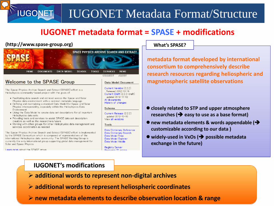
IUGONET Metadata Format/StructureIUGONET metadata format = SPASE + modifications
What’s SPASE?
metadata format developed by international consortium to comprehensively describe research resources regarding heliospheric and magnetospheric satellite observations
closely related to STP and upper atmosphere researches ( easy to use as a base format)
new metadata elements & words appendable (customizable according to our data )
widely-used in VxOs ( possible metadata exchange in the future)
(http://www.spase-group.org)
IUGONET’s modifications additional words to represent non-digital archives
additional words to represent heliospheric coordinates
new metadata elements to describe observation location & range
プレゼンター
プレゼンテーションのノート
We use the SPASE data model/metadata format as the base of the IUGONET metadata format. SPASE is metadata format developed by international consortium to comprehensively describe research resources regarding heliospheric and magnetospheric satellite observations. In addition, we add some modification to SPASE for ground-based observational data.

IUGONET Metadata Database
IUGONET MDB (called IUGONET Type-A) is capable of cross-searching observational data distributed across the IUGONET institutions.
IUGONET Type-A brings a remarkable advancement in accessibility to the observational data and accelerate the interdisciplinary study.
IUGONET Type-A provides a one-stop web services such as searching data, finding interesting events, interactively plotting the data, and leading users to more detailed analysis.
http://search.iugonet.org/
プレゼンター
プレゼンテーションのノート
To access the previous metadata, IUGONET metadata database is suitable.

Analysis Software SPEDAS
• The IUGONET Data Analysis Software (UDAS) is the plug-in software for Space Physics Environment Data Analysis System(SPEDAS), formerly known as THEMIS Data Analysis Software suite (TDAS)
• The IUGONET data (e.g., geomagnetic data, aurora data, radar data, and so forth) and many satellite mission data (THEMIS, GOES, WIND, and ACE) can be handled.
• It is possible to use many routines to visualize and analyze time series data.
• It accesses the IUGONET data through the Internet, and then the data are automatically downloaded onto the user's computer
Relationship between UDAS, SPEDAS, and IDL
SPEDAS/TDAS
プレゼンター
プレゼンテーションのノート
Visualization and data processing are important for our research field. Next topic is development of data analysis software. The IUGONET Data Analysis Software (UDAS) is the plug-in software for Space Physics Environment Data Analysis Software, formerly known as THEMIS Data Analysis Software suite (TDAS). It is possible to use many routines to visualize and analyze time series data. In this lecture, I will call our software SPEDAS.

Outline of Loading/Plotting Data Using SPEDAS
Data can be easily plotted, for example, by only three basis commands with the SPEDAS-CUI tool.
1. Set a time period2. Load *** data3. Plot the loaded data
timespan, ‘yyyy-mm-dd’iug_load_***tplot, +++
If using the GUI tool, only a few simple clicks of your mouse are required to make the same plot as that created by the above command with the CUI tool
Automatic download
Directories for the downloaded data are created automatically.
Data are loaded as tplot variables
Data Servers on the Internet
User PC
data
data
SSL, Berkeley, THEMIS, GBO
CDAWeb, OMNI, ACE, Wind, etc.
data
プレゼンター
プレゼンテーションのノート
The observational data are archived in the data servers in the internet. If you install the SPEDAS, you can easily download the data through the internet by using SPEDAS. One, Two, Three. If using the GUI tools, only a few simple clicks of your mouse are required to procedure the same plot as that created by the above command with the CUI tool.
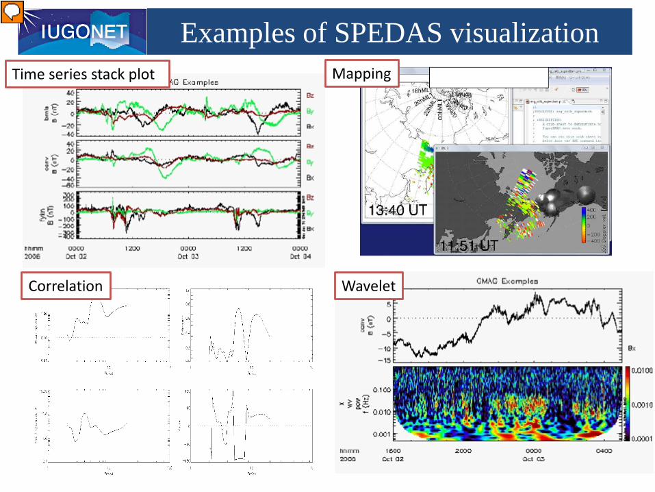
Examples of SPEDAS visualizationTime series stack plot
Wavelet
Mapping
Correlation
プレゼンター
プレゼンテーションのノート
This slide shows examples of SPEDAS visualization. Time series line plot, mapping. And, data processing is also easy. For example, cross correlation and wavelet. Of course, many other useful functions are available.
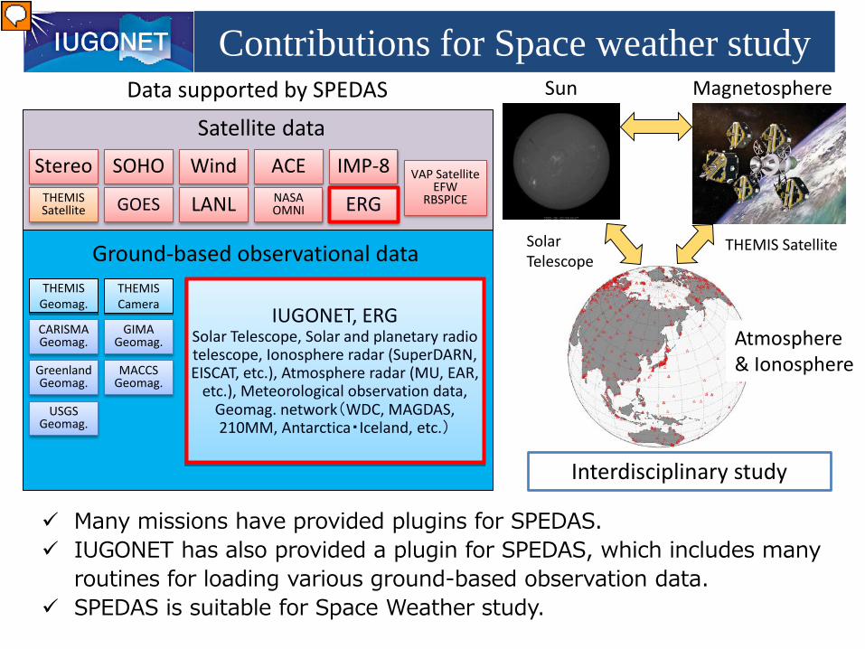
Contributions for Space weather studyMagnetosphereSun
THEMIS Satellite
Atmosphere& Ionosphere
Interdisciplinary study
Solar Telescope
Many missions have provided plugins for SPEDAS. IUGONET has also provided a plugin for SPEDAS, which includes many
routines for loading various ground-based observation data. SPEDAS is suitable for Space Weather study.
THEMISSatellite
THEMISGeomag.
THEMISCamera
Wind ACENASAOMNIGOES LANL
GreenlandGeomag.
MACCSGeomag.
CARISMAGeomag.
GIMAGeomag.
VAP SatelliteEFW
RBSPICE
Stereo
IUGONET, ERGSolar Telescope, Solar and planetary radio telescope, Ionosphere radar (SuperDARN, EISCAT, etc.), Atmosphere radar (MU, EAR,
etc.), Meteorological observation data, Geomag. network(WDC, MAGDAS, 210MM, Antarctica・Iceland, etc.)
USGSGeomag.
ERG
SOHO IMP-8
Satellite data
Ground-based observational data
Data supported by SPEDAS
プレゼンター
プレゼンテーションのノート
This figure shows the data supported by SPEDAS. SPEDAS can treat many kind of satellite- and ground-based observational data. So, SPEDAS is suitable for the interdisciplinary study, such as the space weather.
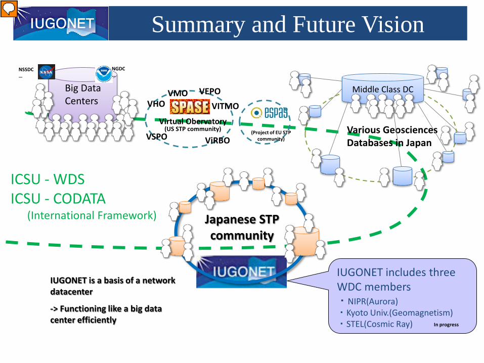
Summary and Future Vision
ICSU - WDSICSU - CODATA
(International Framework)
Big Data Centers
Japanese STP community
Various Geosciences Databases in Japan
Middle Class DC
IUGONET is a basis of a network datacenter
-> Functioning like a big data center efficiently
IUGONET includes three WDC members・NIPR(Aurora)・Kyoto Univ.(Geomagnetism)・STEL(Cosmic Ray) In progress
VMO VEPOVHO VITMO
ViRBOVSPO
Virtual Obervatory(US STP community)
NSSDC…
NGDC…
(Project of EU STP community)
プレゼンター
プレゼンテーションのノート
Currently, not only IUGONET institutes but also other Japanese institutions, such as NAOJ, NICT and Kakioka Magnetic Observatory of JMA, registered metadata in IUGONET MDB. These additions will contribute to efficient interdisciplinary scientific research. It is important to promote interoperability and/or metadata exchange between the database development groups. A memorandum of agreement has been signed with the ESPAS project, which has similar objectives to IUGONET with regard to a framework for formal collaboration. Furthermore, we will be collaborate with other society for example satellites observation, simulations, big data center, and so on with a view for making/linking metadata databases. Any kind of cooperation, metadata input and feedback is welcomed.

Hand on of SPEDAS
プレゼンター
プレゼンテーションのノート
SPEDAS has so many functions. It is difficult to introduce everything in the limited time of this session. Therefore, training in this session is composed of a basic function. If you have what you want to do not included in this course, you can ask or email us after this session.
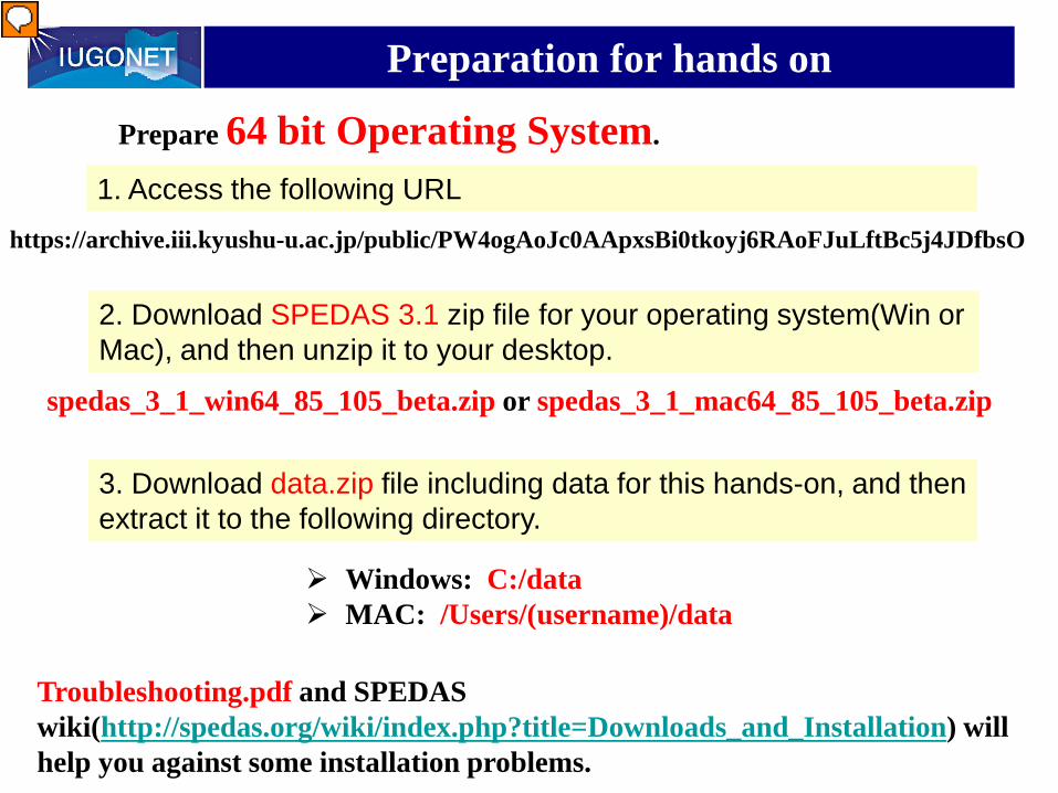
Preparation for hands on
Prepare 64 bit Operating System.
3. Download data.zip file including data for this hands-on, and then extract it to the following directory.
2. Download SPEDAS 3.1 zip file for your operating system(Win or Mac), and then unzip it to your desktop.
1. Access the following URL
Windows: C:/data MAC: /Users/(username)/data
https://archive.iii.kyushu-u.ac.jp/public/PW4ogAoJc0AApxsBi0tkoyj6RAoFJuLftBc5j4JDfbsO
spedas_3_1_win64_85_105_beta.zip or spedas_3_1_mac64_85_105_beta.zip
Troubleshooting.pdf and SPEDAS wiki(http://spedas.org/wiki/index.php?title=Downloads_and_Installation) will help you against some installation problems.
プレゼンター
プレゼンテーションのノート
If you do not download there, please put your hand up. We have USB memories for coping software and data.

Preparation for hands on4. In section 3, you can load and plot your own data on SPEDAS. Please prepare it with the following format.
Supprted format:1. CDF(Common Data Format)
2. AsciiIn this hands-on two format types shown are supported:0) Time series data arranged in the following order (i.e., date, time, and data);-----------------------------------------------------date[0] time[0] ydata1[0] ydata2[0] ydata3[0] …date[0] time[1] ydata1[1] ydata2[1] ydata3[1] …date[0] time[2] ydata1[2] ydata2[2] ydata3[2] …date[0] time[3] ydata1[3] ydata2[3] ydata3[3] …date[0] time[4] ydata1[4] ydata2[4] ydata3[4] …-----------------------------------------------------where, ydata1, ydata2, ydata3, … are the column data.As for the date[] and time[] format string, various formats are acceptable, for example, YYYY-MM-DD/hh:mm:ssyy MM DD hh mm sshh mm ss See example “data/testfile_format0.txt”
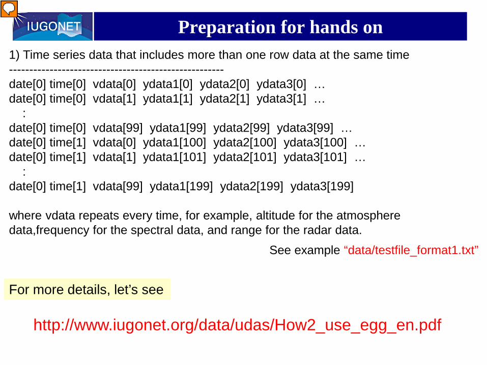
Preparation for hands on1) Time series data that includes more than one row data at the same time-----------------------------------------------------date[0] time[0] vdata[0] ydata1[0] ydata2[0] ydata3[0] …date[0] time[0] vdata[1] ydata1[1] ydata2[1] ydata3[1] …
:date[0] time[0] vdata[99] ydata1[99] ydata2[99] ydata3[99] …date[0] time[1] vdata[0] ydata1[100] ydata2[100] ydata3[100] …date[0] time[1] vdata[1] ydata1[101] ydata2[101] ydata3[101] …
:date[0] time[1] vdata[99] ydata1[199] ydata2[199] ydata3[199]
where vdata repeats every time, for example, altitude for the atmosphere data,frequency for the spectral data, and range for the radar data.
See example “data/testfile_format1.txt”
For more details, let’s see
http://www.iugonet.org/data/udas/How2_use_egg_en.pdf
プレゼンター
プレゼンテーションのノート
If you do not have your data for hands-on, no problem. We prepared one data for practice.

Start of IDL-VM(GUI) tool
[1] Unzip the zipped SPEDAS file.
[2] Double-click the executable file named ‘spedas’ in the directory ‘spedas_v_3/spd_gui’.
Doule-click the executable file named ‘spedas’
[3] IDL Virtual Machine window opens on your PC, so please click the ‘spd_gui’ button.Click the icon
‘spd_gui’.
プレゼンター
プレゼンテーションのノート
If you click the executable file named ‘spedas’, you find another window of IDL-VM. Can you find it? Then, you click the icon named ‘spd_gui’.
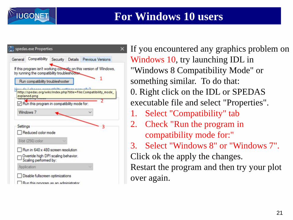
For Windows 10 users
21
If you encountered any graphics problem on Windows 10, try launching IDL in "Windows 8 Compatibility Mode" or something similar. To do that:0. Right click on the IDL or SPEDAS executable file and select "Properties".1. Select "Compatibility" tab2. Check "Run the program in
compatibility mode for:"3. Select "Windows 8" or "Windows 7".Click ok the apply the changes.Restart the program and then try your plot over again.

Start of IDL-VM(GUI) tool
Ready?
プレゼンター
プレゼンテーションのノート
When you finish downloading this file, you extract it and open the directory named spd_gui. If you click the executable file named ‘spedas’, you find another window of IDL-VM. Then, you click the icon named ‘spd_gui’.
How to Use SPEDASpart1
・Load data・Plot data・Save figure, data, and your work
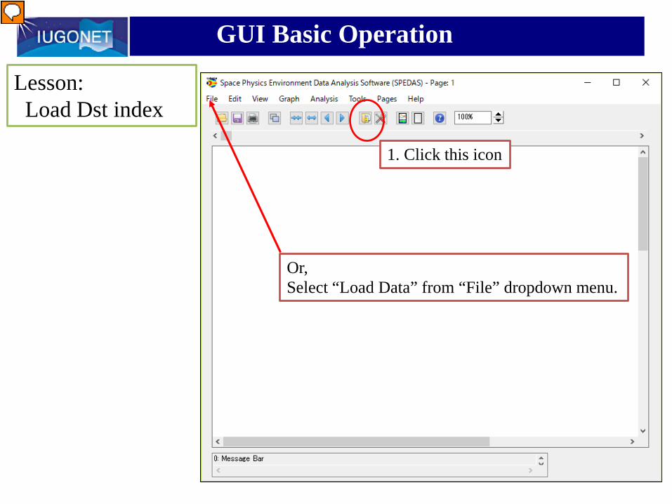
GUI Basic Operation
Lesson:Load Dst index
1. Click this icon
Or,Select “Load Data” from “File” dropdown menu.
プレゼンター
プレゼンテーションのノート
First lesson, we will learn how to load data. The example data is Dst index. This index is well known as the indicator of geomagnetic storm.
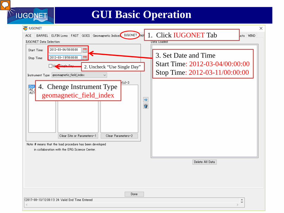
4. Chenge Instrument Typegeomagnetic_field_index
GUI Basic Operation
3. Set Date and TimeStart Time: 2012-03-04/00:00:00Stop Time: 2012-03-11/00:00:00
1. Click IUGONET Tab
2. Uncheck “Use Single Day”
プレゼンター
プレゼンテーションのノート
There are many tabs. If you want to load THEMIS satellite data, click THEMIS. At this time we will use IUGONET tab.
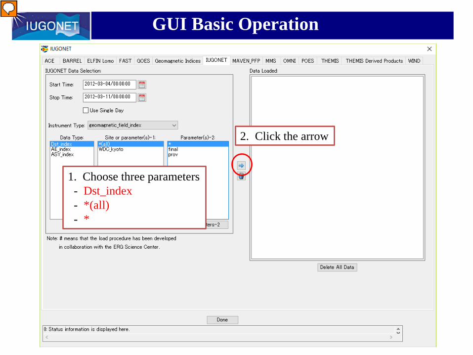
1. Choose three parameters- Dst_index- *(all)- *
GUI Basic Operation
2. Click the arrow
プレゼンター
プレゼンテーションのノート
And then, choose the parameter

Display of Data Use Policy
GUI Basic Operation
1. Click“OK”
プレゼンター
プレゼンテーションのノート
You can get this window, right? This is the rules of each data. These rules are different from each institute. Read it carefully, and if you will agree with the rules, click OK

GUI Basic Operation
2. Click“Done”
1. Data was loaded successfully!
プレゼンター
プレゼンテーションのノート
Loaded data is located at the right side window. Finished? Not finished? Please support around you. Teaching to others leads to your skill improvement.
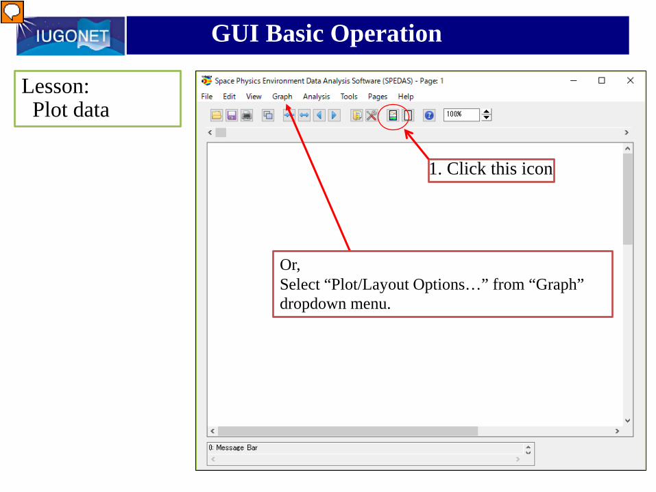
Lesson:Plot data
1. Click this icon
GUI Basic Operation
Or,Select “Plot/Layout Options…” from “Graph” dropdown menu.
プレゼンター
プレゼンテーションのノート
Second lesson is how to plot data. Visualization is very important.

1. Select data which you want to plot:wdc_mag_dst_prov
GUI Basic Operation
2. Click “Line”
プレゼンター
プレゼンテーションのノート
In Left panel, we can see data which you loaded at the previous section. If you can click this + icon, the tree is expanded, and you can see the details of data.

1. Selected variable name is added to this box
GUI Basic Operation
2. Click OK
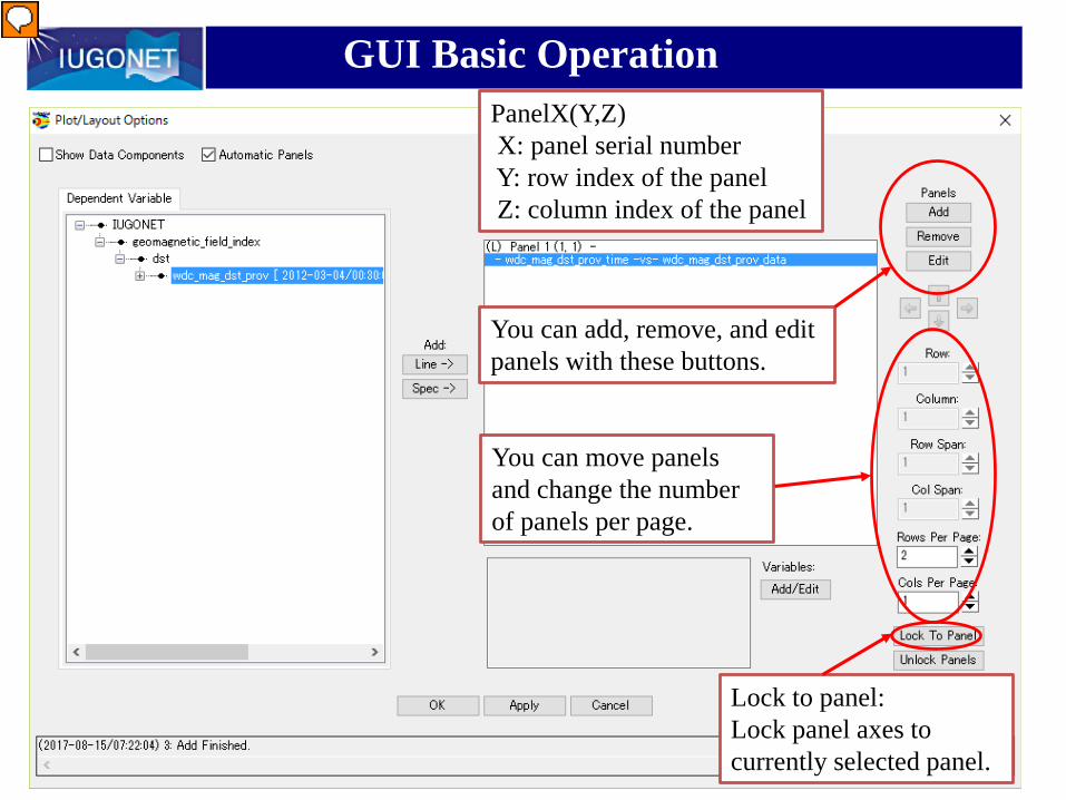
GUI Basic OperationPanelX(Y,Z)X: panel serial numberY: row index of the panelZ: column index of the panel
Lock to panel:Lock panel axes to currently selected panel.
You can move panels and change the number of panels per page.
You can add, remove, and edit panels with these buttons.
プレゼンター
プレゼンテーションのノート
This is a short tips of this panel.
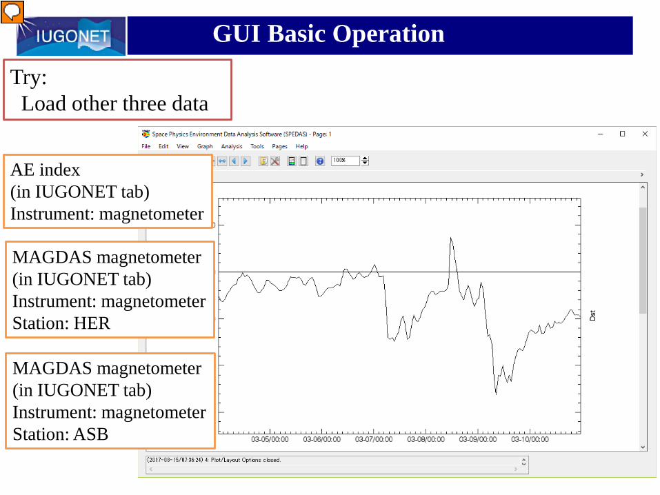
Try: Load other three data
AE index(in IUGONET tab)Instrument: magnetometer
MAGDAS magnetometer(in IUGONET tab)Instrument: magnetometerStation: HER
GUI Basic Operation
MAGDAS magnetometer(in IUGONET tab)Instrument: magnetometerStation: ASB
プレゼンター
プレゼンテーションのノート
Now, we learned how to load and plot data. Let’s try to load these three plot. 5 minutes thinking time
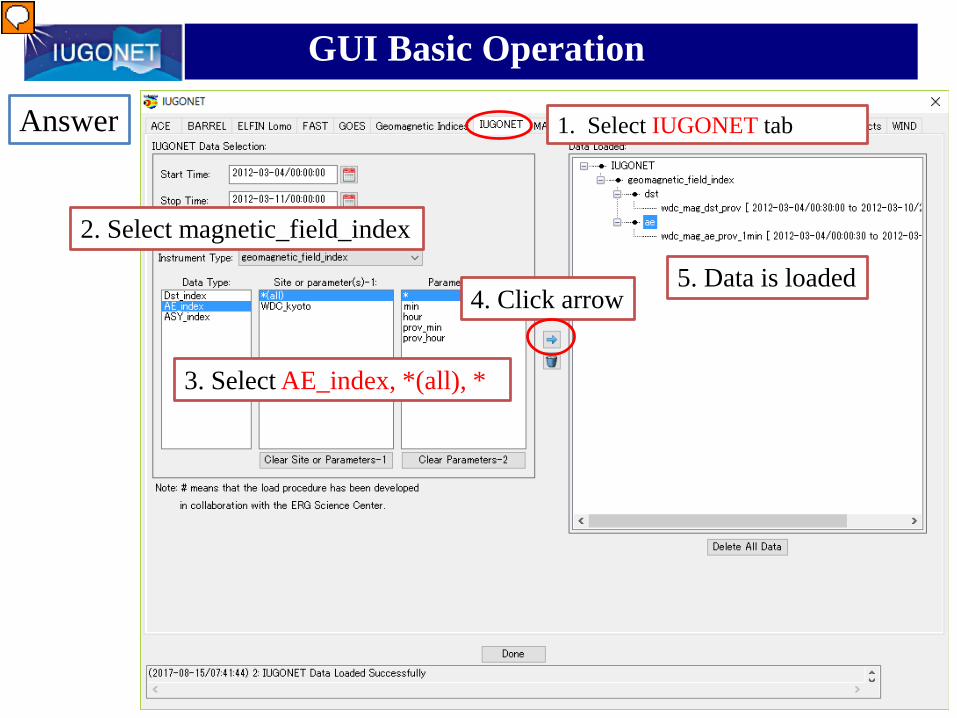
Answer
2. Select magnetic_field_index
3. Select AE_index, *(all), *
5. Data is loaded
GUI Basic Operation
1. Select IUGONET tab
4. Click arrow
プレゼンター
プレゼンテーションのノート
Answer part

1. Select geomagnetic_field_fluxgate
4. Data is loaded
GUI Basic Operation
Answer
2. Select magdas#, asb & her, *
3. Click arrow
5. Click Done
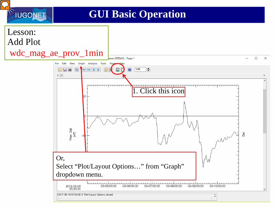
GUI Basic OperationLesson: Add Plot wdc_mag_ae_prov_1min
Or,Select “Plot/Layout Options…” from “Graph” dropdown menu.
1. Click this icon
プレゼンター
プレゼンテーションのノート
Next, let’s plot the second data

4. Data are added
2. Select wdc_mag_ae_prov_1min
1. Click Add
GUI Basic Operation
3. Click “Line”
5. Click OK
GUI Basic Operation
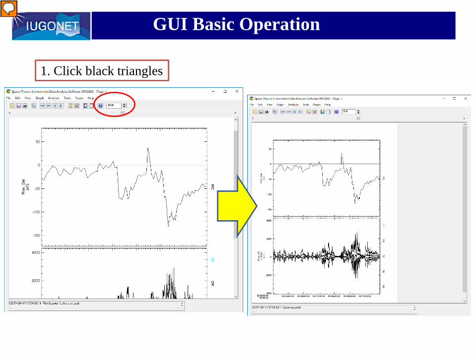
1. Click black triangles
プレゼンター
プレゼンテーションのノート
To expand or reduce the figure, click these black triangles
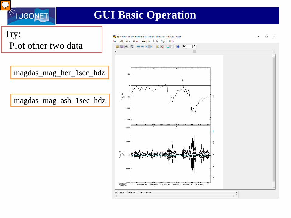
GUI Basic OperationTry: Plot other two data
magdas_mag_her_1sec_hdz
magdas_mag_asb_1sec_hdz
プレゼンター
プレゼンテーションのノート
Let’s try
GUI Basic Operation
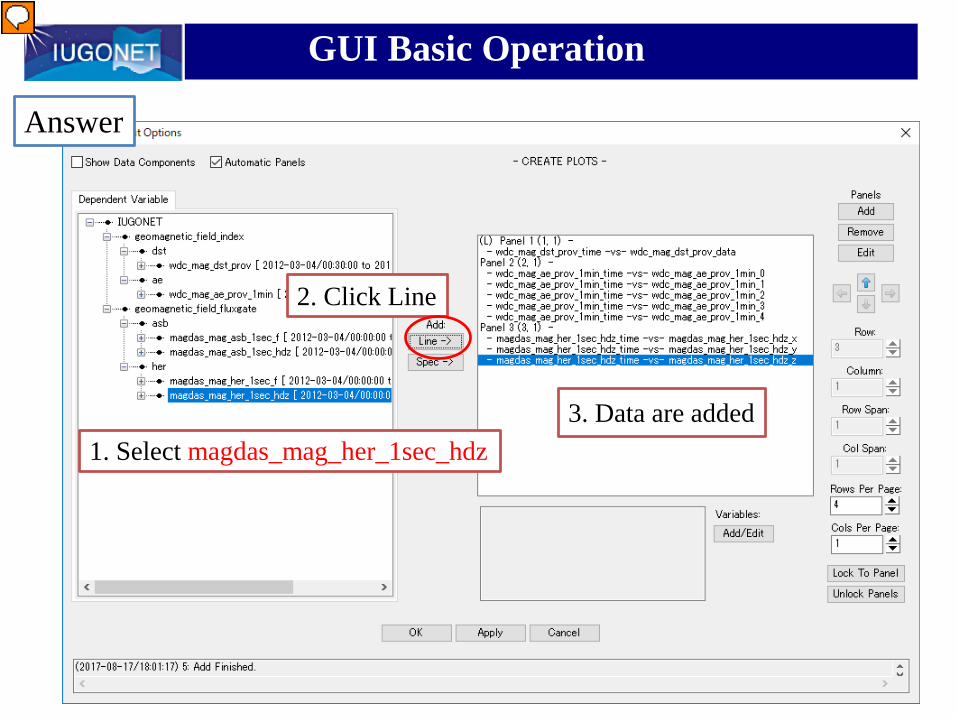
Answer
3. Data are added1. Select magdas_mag_her_1sec_hdz
2. Click Line
プレゼンター
プレゼンテーションのノート
Answer
GUI Basic Operation
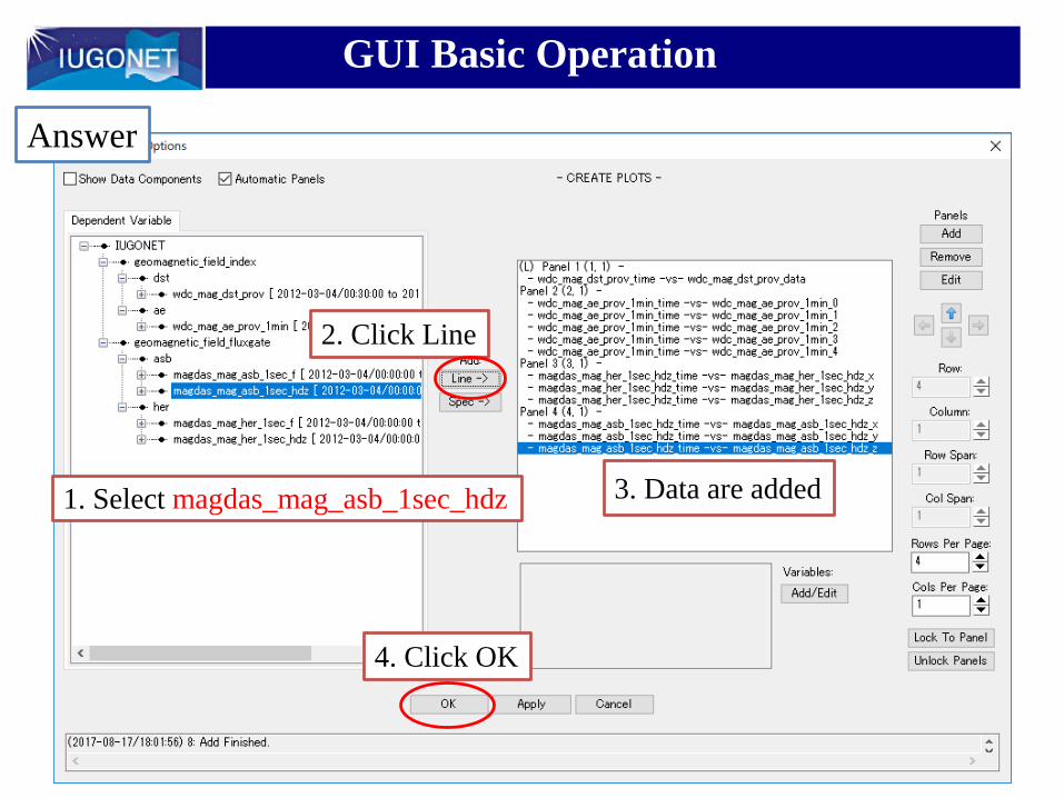
Answer
3. Data are added1. Select magdas_mag_asb_1sec_hdz
2. Click Line
4. Click OK

GUI Basic Operation
プレゼンター
プレゼンテーションのノート
Can you get this plot? This is very big noise. But, no problem, we will remove this noise later.

GUI Basic Operation
Lesson: Save plot as figure
1. SelectFile – Export To Image File
2. Select save folder
2. Input file name and select format (by extension)
3. Click “save”
プレゼンター
プレゼンテーションのノート
Next lesson is save this plot as figure.
GUI Basic Operation
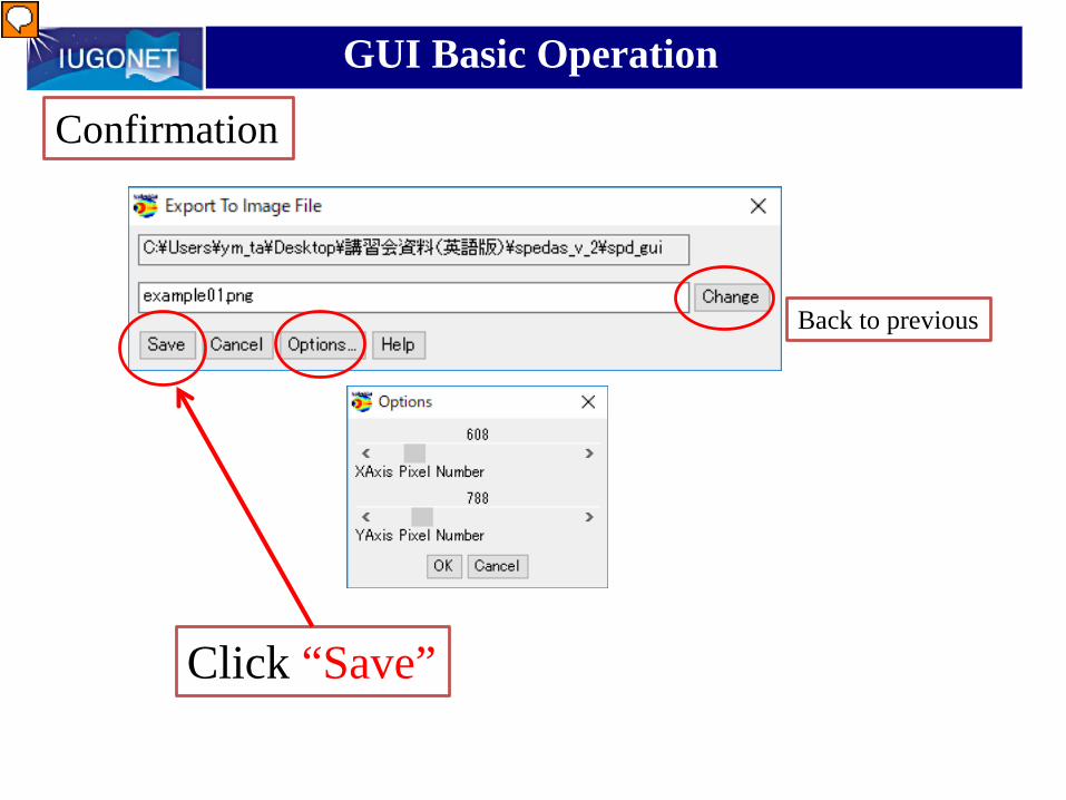
Confirmation
Back to previous
Click “Save”
プレゼンター
プレゼンテーションのノート
Click option, you can change file size of the figure
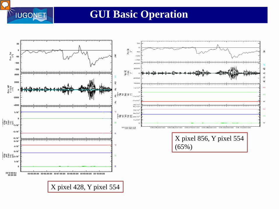
GUI Basic Operation
X pixel 428, Y pixel 554
X pixel 856, Y pixel 554(65%)
プレゼンター
プレゼンテーションのノート
This is example. Left is landscape and right is portlate

GUI Basic Operation
Lesson: Save data as ascii
1. SelectFile – Save Data As

GUI Basic Operation
4. check this box
1. Select data which you want to savemagdas_mag_her_1sec_hdz_x
5. Click Save
6. Select save folder
7. Input file name (data is saved in csv format)
8. Click “save”
2. check this box
3. Select time interval

GUI Basic Operation
An ascii data file was successfully saved!!!
プレゼンター
プレゼンテーションのノート
You can read saved asci data by using your proper software. For example, MS Excel can plot the magdas data saved as ascii file.
GUI Basic Operation
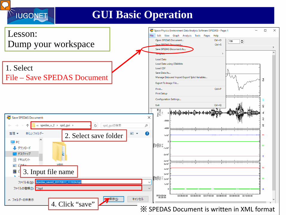
Lesson: Dump your workspace
1. SelectFile – Save SPEDAS Document
2. Select save folder
3. Input file name
4. Click “save”※ SPEDAS Document is written in XML format
プレゼンター
プレゼンテーションのノート
5 minutes break

Coffee Break…
How to Use SPEDASpart2
・Restore your work・Manage axis・Process and data
プレゼンター
プレゼンテーションのノート
Break is over. I get the hands on started again.
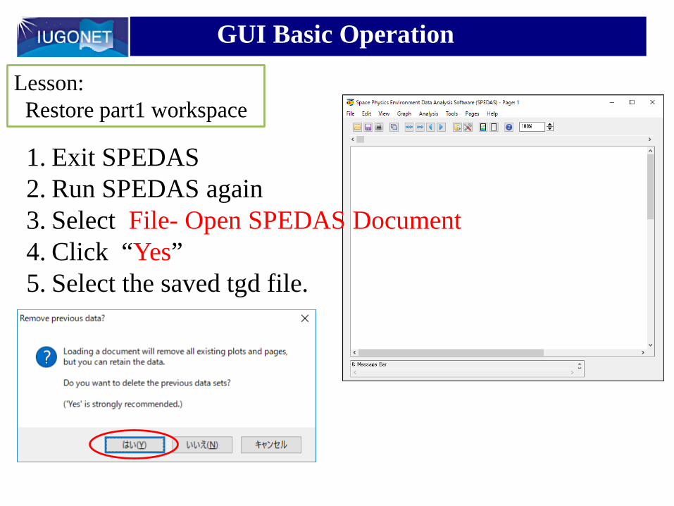
GUI Basic Operation
Lesson:Restore part1 workspace
1. Exit SPEDAS2. Run SPEDAS again3. Select File- Open SPEDAS Document4. Click “Yes”5. Select the saved tgd file.

GUI Basic Operation
Lesson:Remove plot
1. Select Graph – Plot/Layout Options
プレゼンター
プレゼンテーションのノート
In fact, the third panel has four type of data. We need only one data, so let’s remove unused data.
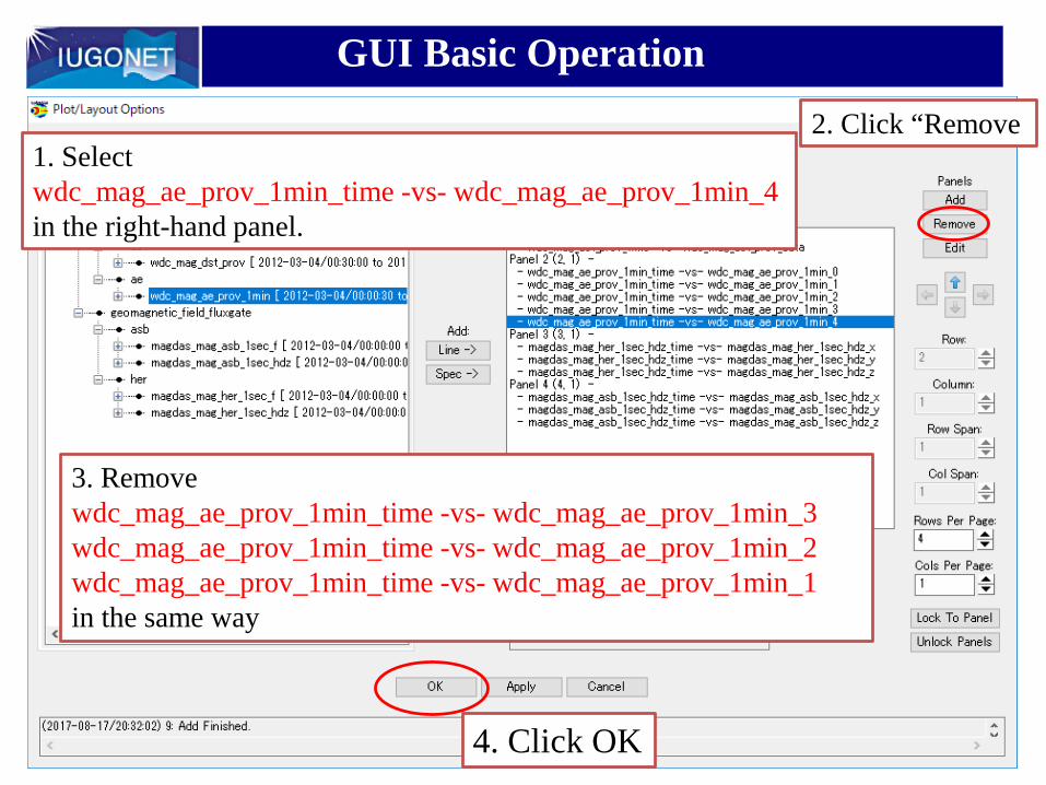
GUI Basic Operation
1. Select wdc_mag_ae_prov_1min_time -vs- wdc_mag_ae_prov_1min_4in the right-hand panel.
2. Click “Remove
3. Removewdc_mag_ae_prov_1min_time -vs- wdc_mag_ae_prov_1min_3wdc_mag_ae_prov_1min_time -vs- wdc_mag_ae_prov_1min_2wdc_mag_ae_prov_1min_time -vs- wdc_mag_ae_prov_1min_1in the same way
4. Click OK
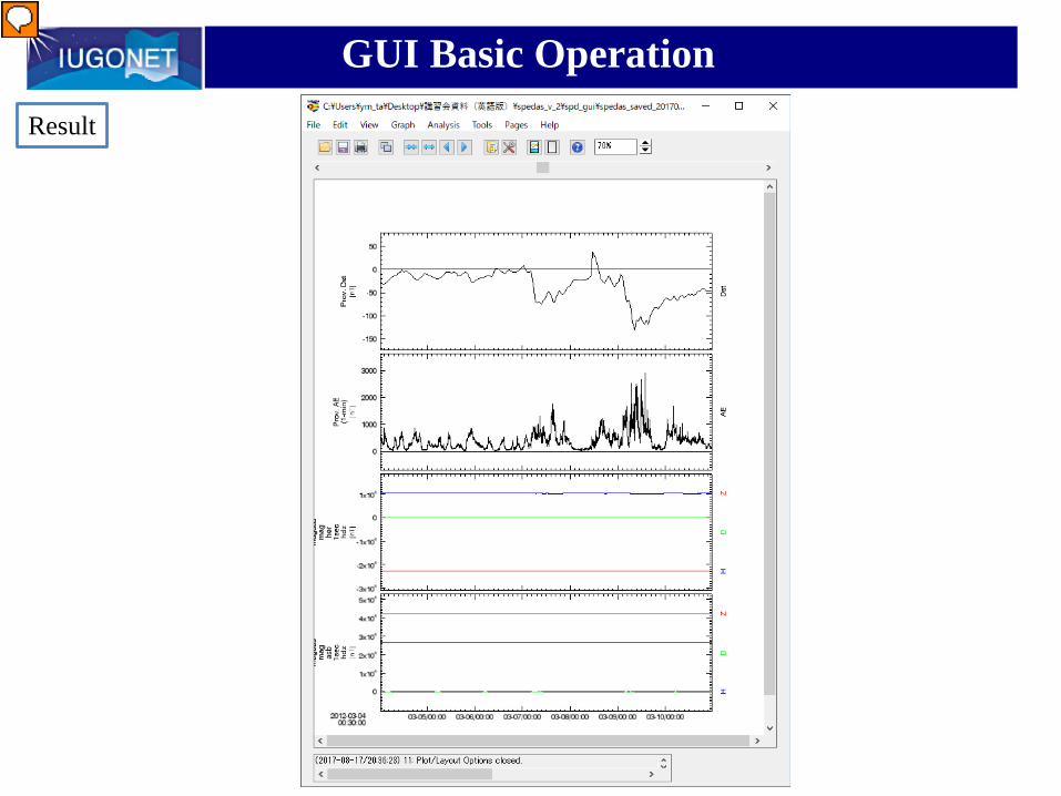
GUI Basic OperationResult
プレゼンター
プレゼンテーションのノート
Only H component remain
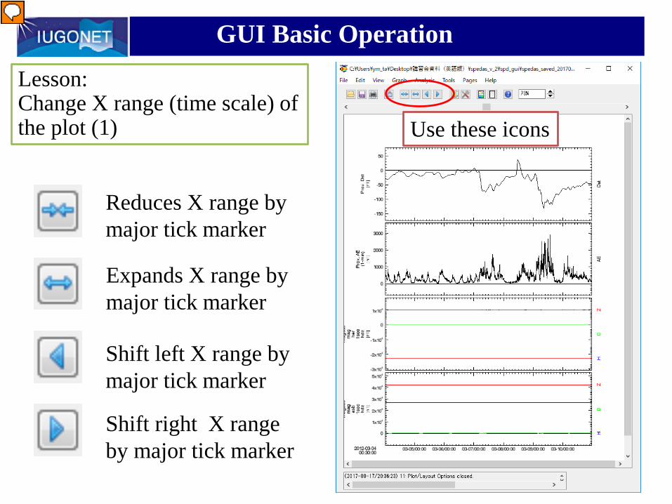
GUI Basic Operation
Lesson: Change X range (time scale) of the plot (1) Use these icons
Reduces X range by major tick marker
Expands X range by major tick marker
Shift left X range by major tick marker
Shift right X range by major tick marker
プレゼンター
プレゼンテーションのノート
Next lesson is change X range of the plot. First is simple method. Use these icons. The meaning of these icons are as follows
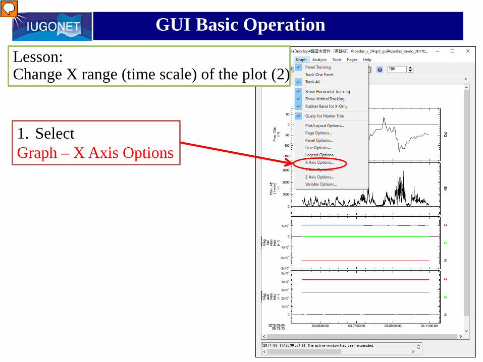
GUI Basic Operation
Lesson: Change X range (time scale) of the plot (2)
1. Select Graph – X Axis Options
プレゼンター
プレゼンテーションのノート
Second is the detailed method

GUI Basic Operation
2. Select Fixed Range
3. Change valuesMin 2012-03-06/00:00:00.000Max 2012-03-11/00:00:00.000
1. Select Panel (If panel is locked, use “Apply to All Panels”.)
4. Click "Apply to All Panels”
GUI Basic Operation
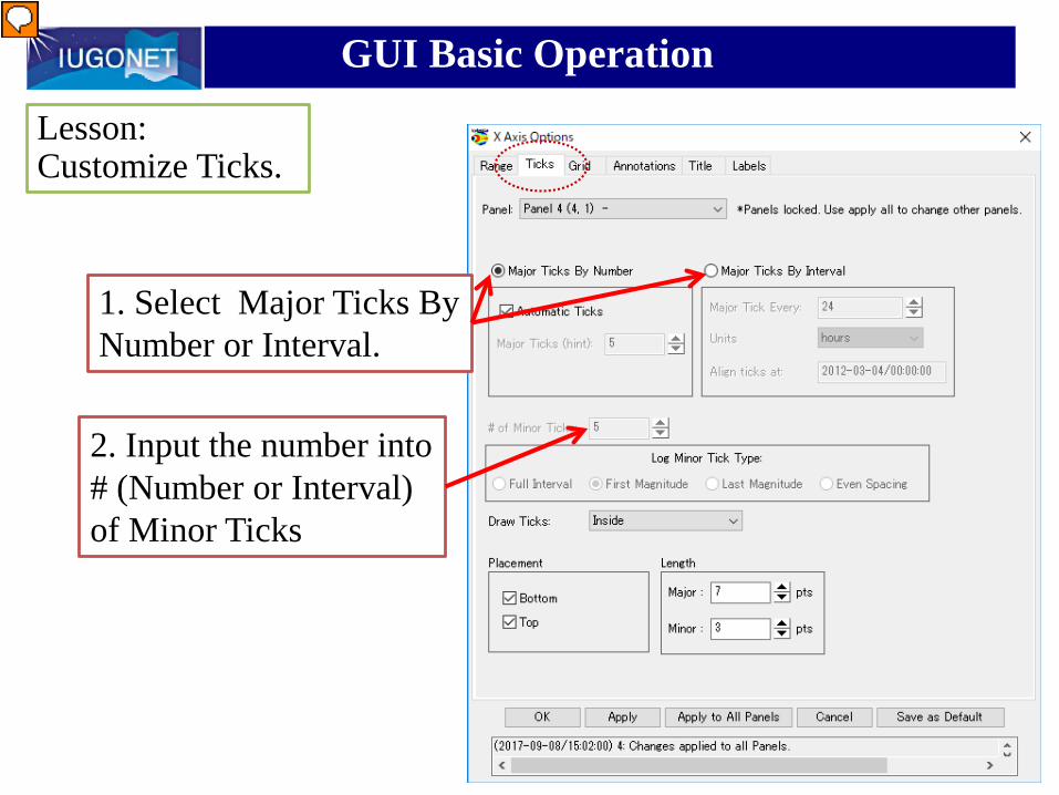
Lesson:Customize Ticks.
1. Select Major Ticks By Number or Interval.
2. Input the number into # (Number or Interval) of Minor Ticks
プレゼンター
プレゼンテーションのノート
In this lesson, select the left one
GUI Basic Operation
60
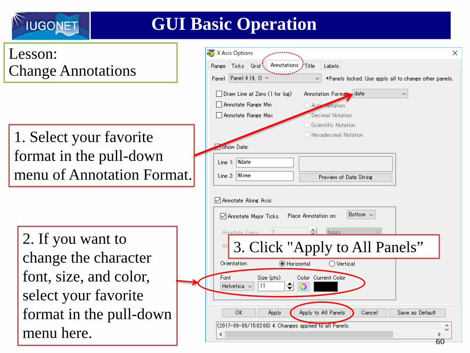
1. Select your favorite format in the pull-down menu of Annotation Format.
2. If you want to change the character font, size, and color, select your favorite format in the pull-down menu here.
3. Click "Apply to All Panels”
Lesson: Change Annotations
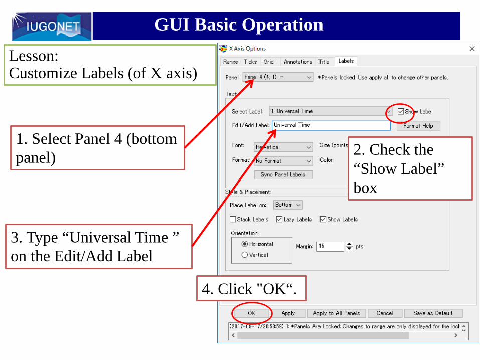
GUI Basic OperationLesson:Customize Labels (of X axis)
3. Type “Universal Time ” on the Edit/Add Label
2. Check the “Show Label” box
4. Click "OK“.
1. Select Panel 4 (bottom panel)

GUI Basic OperationResult
プレゼンター
プレゼンテーションのノート
Only H component remain
GUI Basic Operation
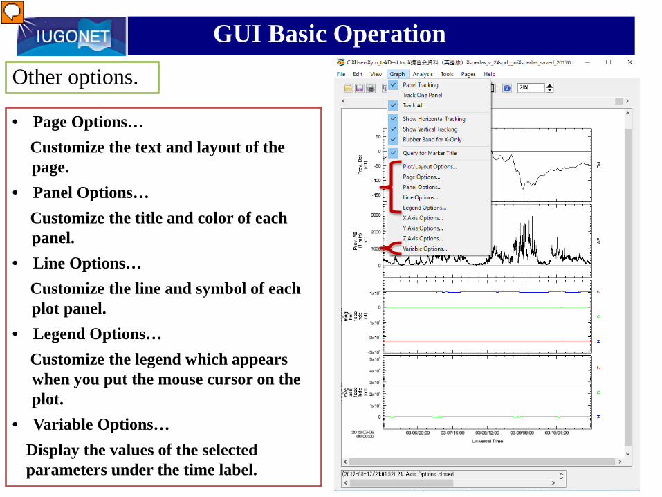
• Page Options…Customize the text and layout of the page.
• Panel Options…Customize the title and color of each panel.
• Line Options…Customize the line and symbol of each plot panel.
• Legend Options…Customize the legend which appears when you put the mouse cursor on the plot.
• Variable Options…Display the values of the selected parameters under the time label.
Other options.
プレゼンター
プレゼンテーションのノート
There are other many options for graphics. For example… Let’s try these options after this hands-on training

GUI Basic Operation
Lesson: Reset X range (time scale)
1. Select X Axis Options
プレゼンター
プレゼンテーションのノート
Before next lesson, reset X range.

GUI Basic Operation
2. Select Auto Range
3. Click “OK”
1. Select (L) Panel 1(1, 1) -
GUI Basic Operation
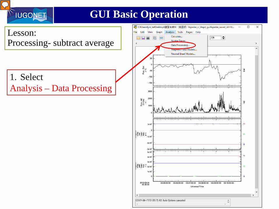
Lesson: Processing- subtract average
1. Select Analysis – Data Processing
プレゼンター
プレゼンテーションのノート
Next is data processing. This software has many data processing functions. In this lesson, let’s remove this noise
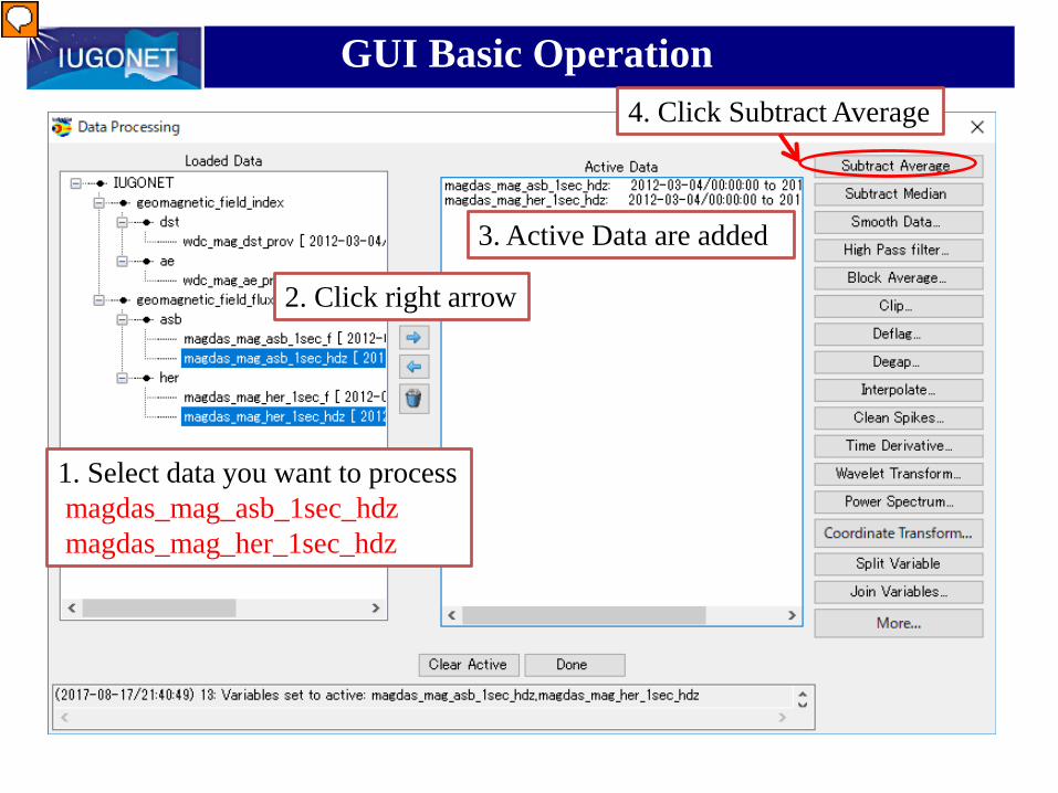
GUI Basic Operation
2. Click right arrow
3. Active Data are added
1. Select data you want to processmagdas_mag_asb_1sec_hdzmagdas_mag_her_1sec_hdz
4. Click Subtract Average
プレゼンター
プレゼンテーションのノート
Threshold indicate X value smoothing width indicate Y value
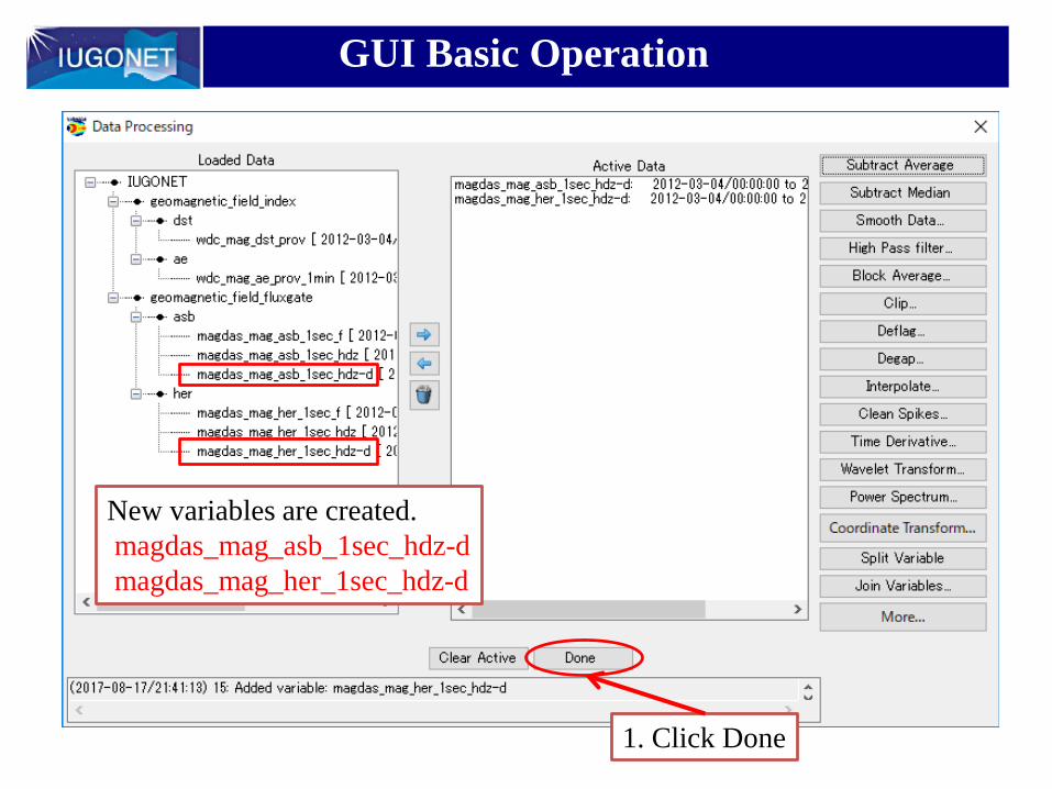
GUI Basic Operation
1. Click Done
New variables are created.magdas_mag_asb_1sec_hdz-dmagdas_mag_her_1sec_hdz-d

GUI Basic OperationOpen “Plot/Layout Options”
2. Select magdas_mag_her_1sec_hdz-d
3. Click line
4. Data are added
6. Click OK
5. Then, add the other variable,magdas_mag_asb_1sec_hdz-dto panel in the same way.
1. Remove Panel 3 and 4

GUI Basic Operation
Subtracted average!
GUI Basic Operation
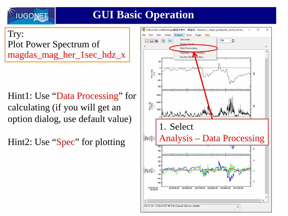
Try: Plot Power Spectrum ofmagdas_mag_her_1sec_hdz_x
1. Select Analysis – Data Processing
Hint1: Use “Data Processing” for calculating (if you will get an option dialog, use default value)
Hint2: Use “Spec” for plotting

GUI Basic Operation
2. Active Data is removed
1. Click Clear Active
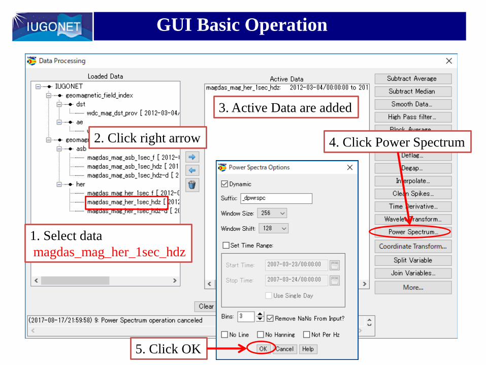
GUI Basic Operation
2. Click right arrow
3. Active Data are added
4. Click Power Spectrum
5. Click OK
1. Select datamagdas_mag_her_1sec_hdz
GUI Basic Operation
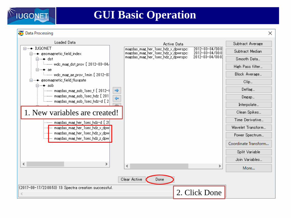
1. New variables are created!
2. Click Done
GUI Basic Operation
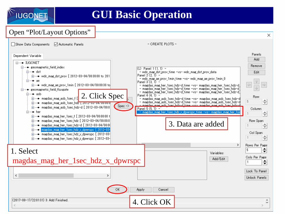
1. Select magdas_mag_her_1sec_hdz_x_dpwrspc
2. Click Spec
3. Data are added
4. Click OK
Open “Plot/Layout Options”
GUI Basic Operation
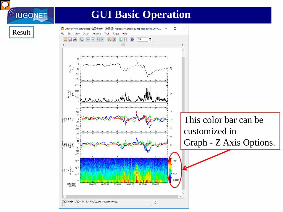
This color bar can be customized in Graph - Z Axis Options.
Result
プレゼンター
プレゼンテーションのノート
Last lesson of today’s hands-on is calculator. If you want to process data by using your own method, you can make equation and apply it to data.
GUI Basic Operation
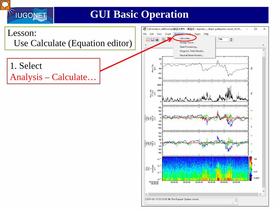
Lesson: Use Calculate (Equation editor)
1. Select Analysis – Calculate…
プレゼンター
プレゼンテーションのノート
Last lesson of today’s hands-on is calculator. If you want to process data by using your own method, you can make equation and apply it to data.
GUI Basic Operation
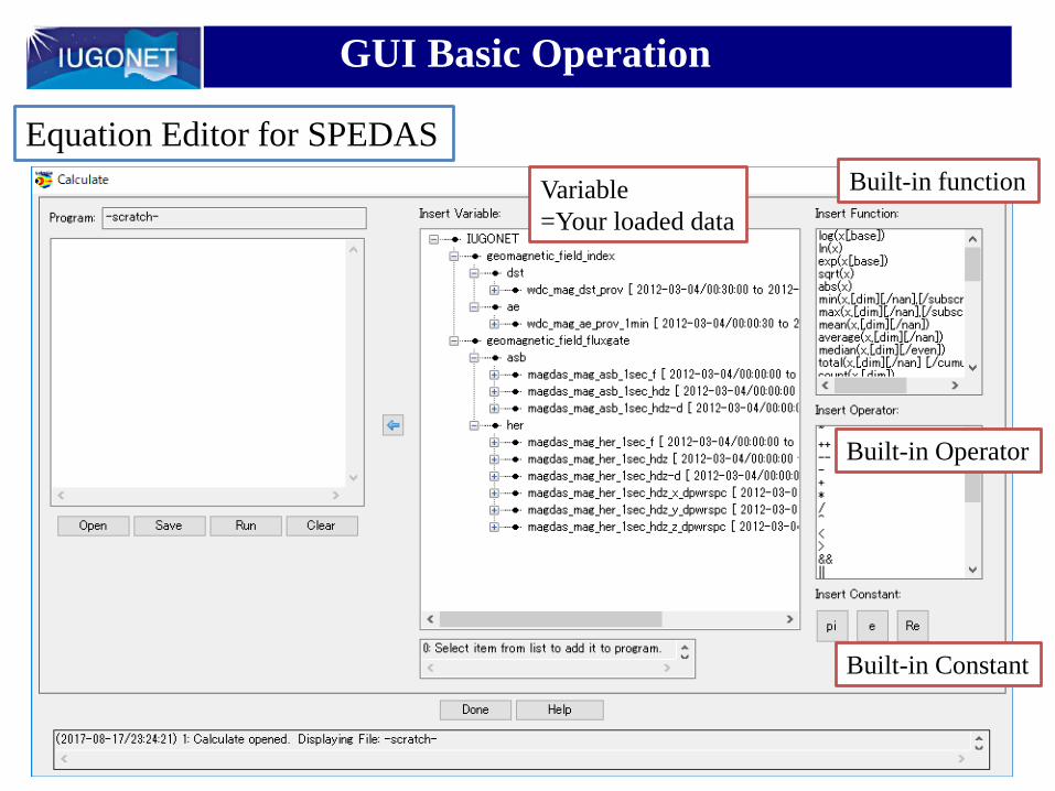
Equation Editor for SPEDASVariable=Your loaded data
Built-in function
Built-in Operator
Built-in Constant

GUI Basic OperationLesson:Make an equation using the loaded variables.
Type variable/function/Operator/Constant, and make equationA = B + C - D…
Note:Enclose the tplot variable in double quotation marks

GUI Basic OperationLesson:Make an equation using the loaded variables.
3. Variable is added
2. Click arrow
Then, try to add the offset (+200) tomagdas_mag_her_1sec_hdz-d_x
and plot on new panel.
1. Select magdas_mag_her_1sec_hdz-d_x
プレゼンター
プレゼンテーションのノート
Clear
GUI Basic Operation
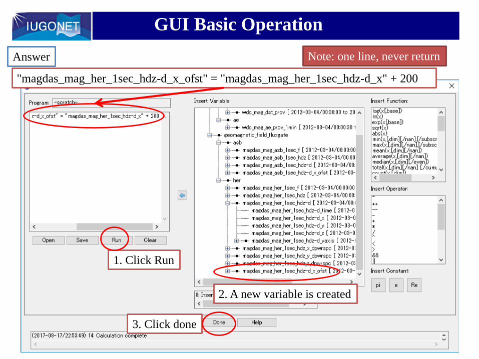
1. Click Run
2. A new variable is created
3. Click done
Answer Note: one line, never return
"magdas_mag_her_1sec_hdz-d_x_ofst" = "magdas_mag_her_1sec_hdz-d_x" + 200
GUI Basic Operation
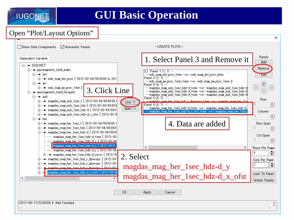
3. Click Line
4. Data are added
Open “Plot/Layout Options”
1. Select Panel 3 and Remove it
2. Select magdas_mag_her_1sec_hdz-d_ymagdas_mag_her_1sec_hdz-d_x_ofst

GUI Basic Operation
2. Panel 6 is changed to (3, 1)
Open “Plot/Layout Options”
1. Change the value of Row to 3
3. Click OK
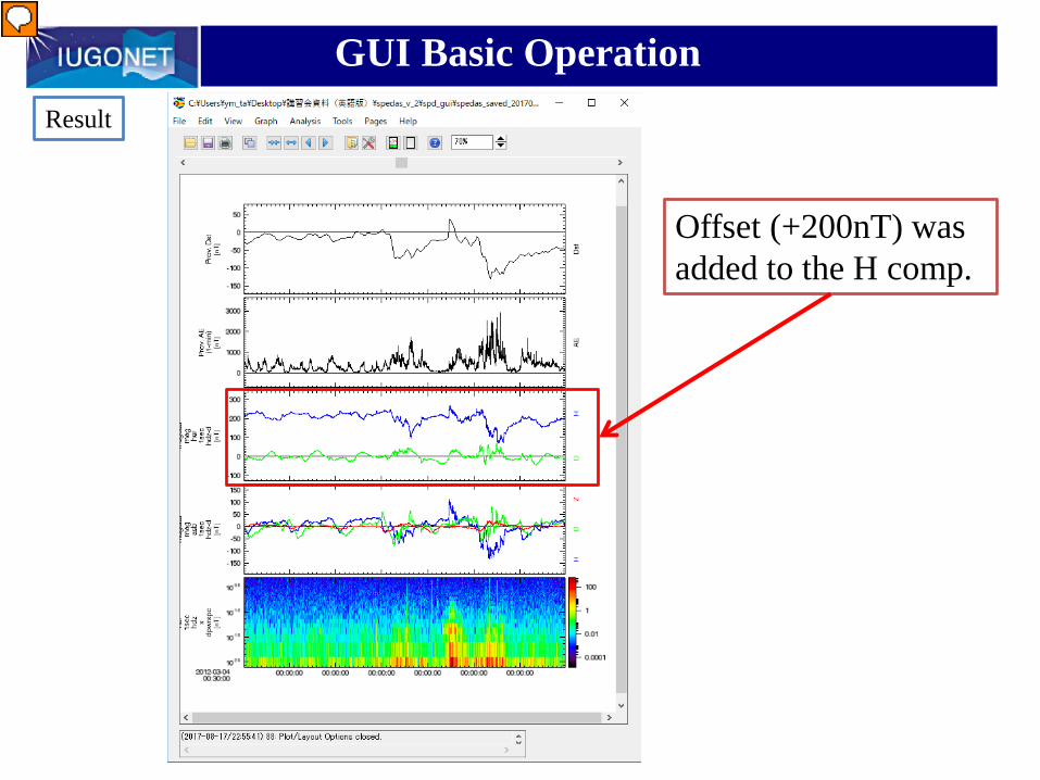
GUI Basic OperationResult
Offset (+200nT) was added to the H comp.
プレゼンター
プレゼンテーションのノート
Last lesson of today’s hands-on is calculator. If you want to process data by using your own method, you can make equation and apply it to data.

GUI Basic Operation
Try: Expand the plot using the mouse.
A new page opens
By left-click and drag the mouse
How to Use SPEDASpart3
・Additional data loading
プレゼンター
プレゼンテーションのノート
Break is over. I get the hands on started again.
GUI Basic Operation
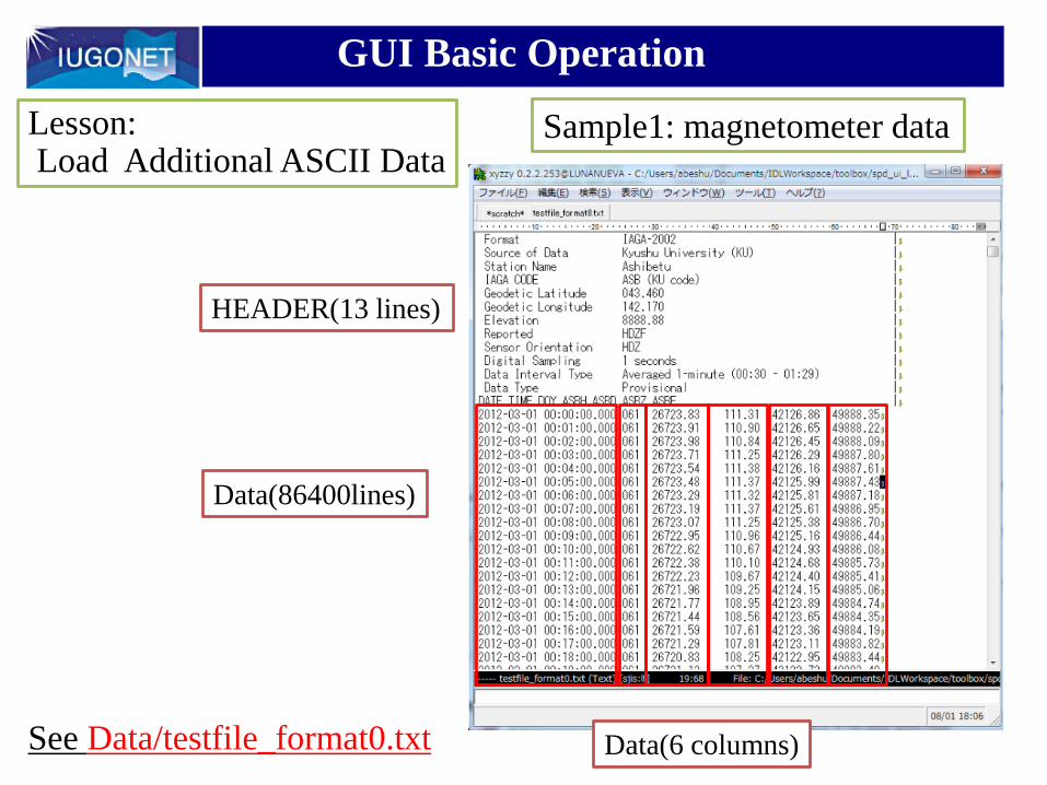
Lesson: Load Additional ASCII Data
Sample1: magnetometer data
HEADER(13 lines)
Data(86400lines)
Data(6 columns)See Data/testfile_format0.txt
GUI Basic Operation
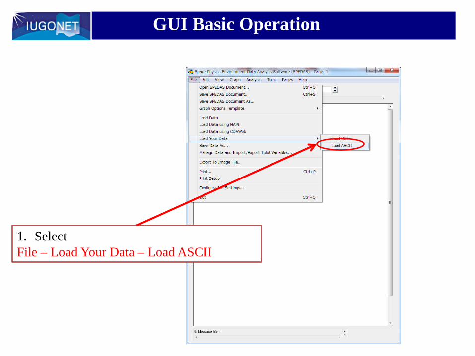
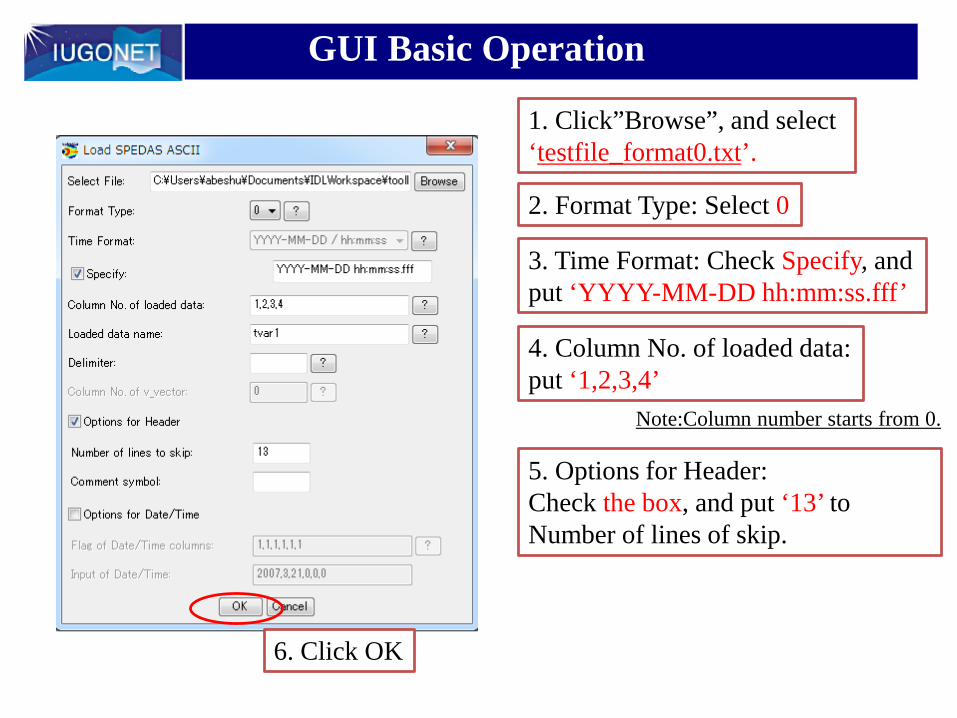
1. Select File – Load Your Data – Load ASCII
GUI Basic Operation
1. Click”Browse”, and select ‘testfile_format0.txt’.
2. Format Type: Select 0
3. Time Format: Check Specify, andput ‘YYYY-MM-DD hh:mm:ss.fff’
4. Column No. of loaded data:put ‘1,2,3,4’
Note:Column number starts from 0.
5. Options for Header:Check the box, and put ‘13’ to Number of lines of skip.
6. Click OK
GUI Basic Operation
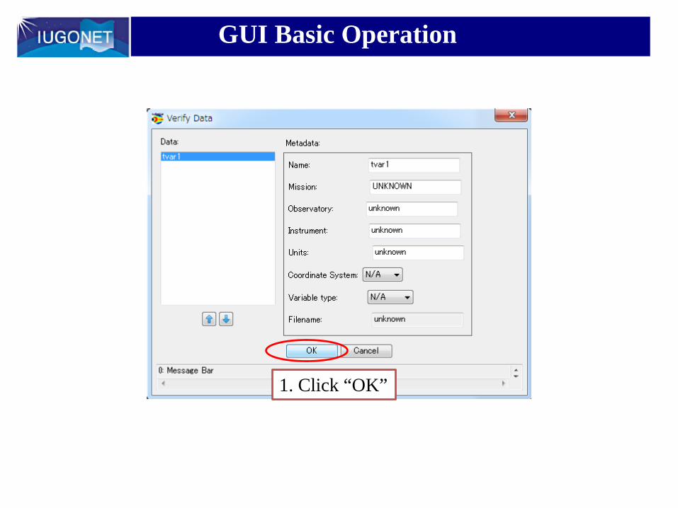
1. Click “OK”
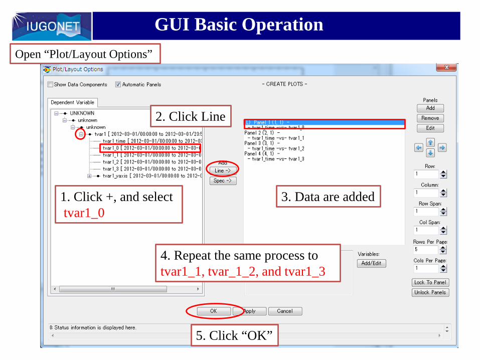
GUI Basic OperationOpen “Plot/Layout Options”
2. Click Line
3. Data are added
4. Repeat the same process totvar1_1, tvar_1_2, and tvar1_3
5. Click “OK”
1. Click +, and select tvar1_0
GUI Basic Operation
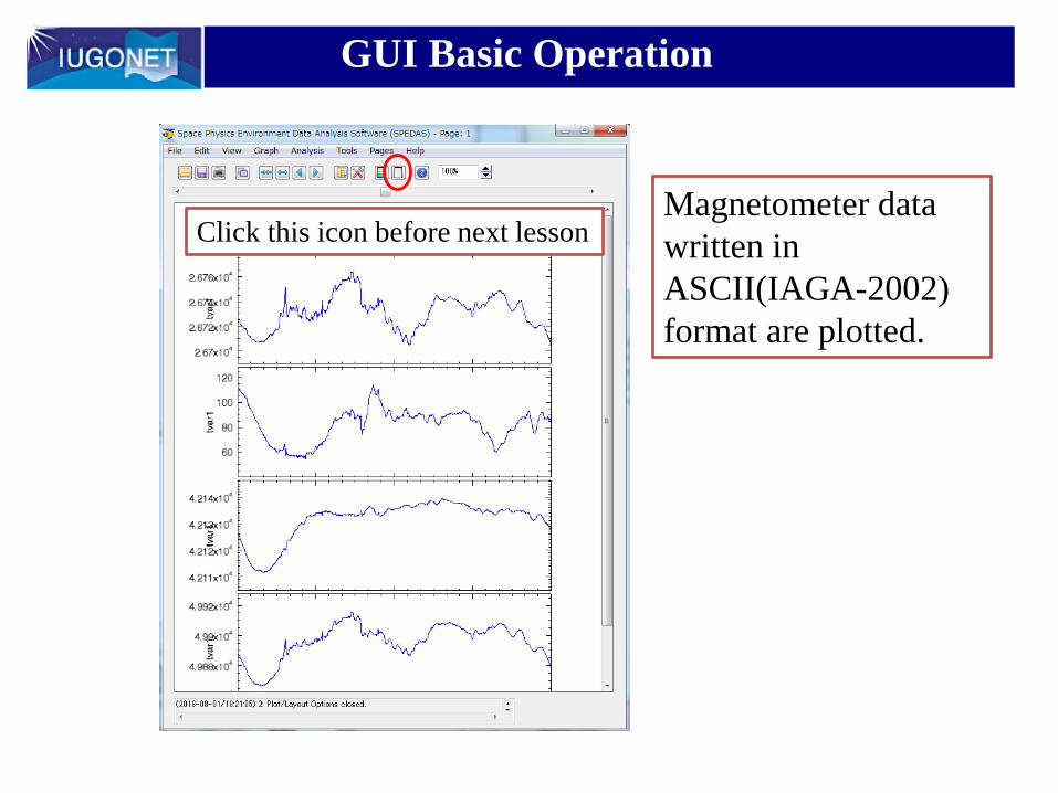
Magnetometer data written in ASCII(IAGA-2002) format are plotted.
Click this icon before next lesson
GUI Basic Operation
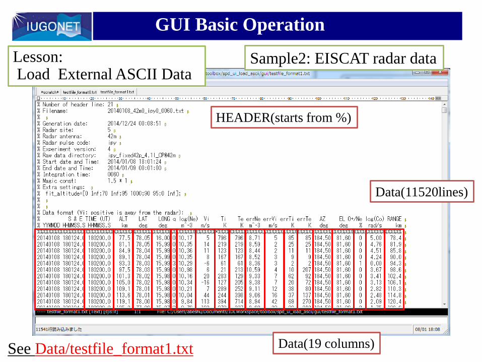
Lesson: Load External ASCII Data
Sample2: EISCAT radar data
HEADER(starts from %)
Data(11520lines)
See Data/testfile_format1.txt Data(19 columns)

GUI Basic OperationOpen File – Load Your Data – Load ASCII 1. Click”Browse”, and select
‘testfile_format1.txt’.
2. Format Type: Select 1
3. Time Format: Check Specify, andput ‘YYYY-MM-DD hh:mm:ss.f’
4. Column No. of loaded data:put ‘5,6,7,8’
7. Options for Header:Check the box, and put ‘%’ to Comment symbol5. Click OK
5. Loaded data name:put ‘Ne, Vi, Ti, Te’
6. Column No. of v_vector:put ‘1’

GUI Basic Operation
1. Click “OK”
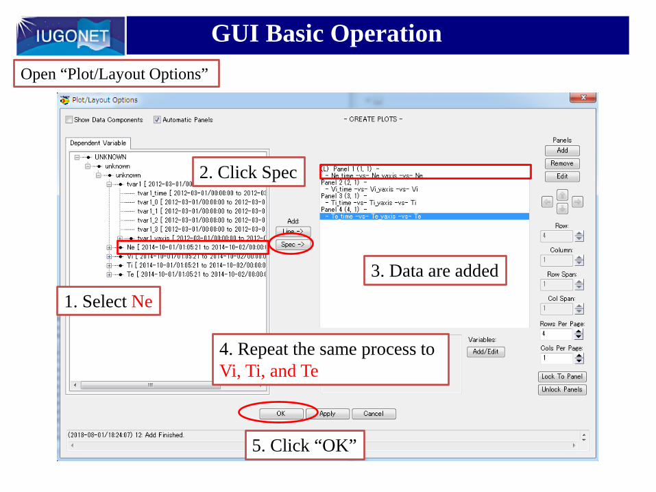
GUI Basic OperationOpen “Plot/Layout Options”
2. Click Spec
3. Data are added
1. Select Ne
4. Repeat the same process to Vi, Ti, and Te
5. Click “OK”

GUI Basic Operation
EISCAT radar data written in ASCII format are plotted in spectrogram.
Click this icon before next lesson
GUI Basic Operation
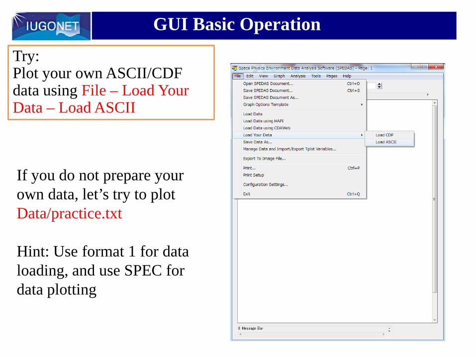
Try: Plot your own ASCII/CDF data using File – Load Your Data – Load ASCII
If you do not prepare your own data, let’s try to plotData/practice.txt
Hint: Use format 1 for data loading, and use SPEC for data plotting
GUI Basic Operation
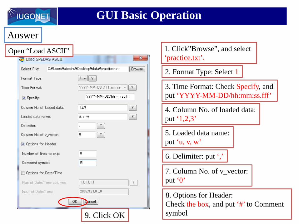
1. Click”Browse”, and select ‘practice.txt’.
2. Format Type: Select 1
3. Time Format: Check Specify, andput ‘YYYY-MM-DD/hh:mm:ss.fff’
4. Column No. of loaded data:put ‘1,2,3’
9. Click OK
8. Options for Header:Check the box, and put ‘#’ to Comment symbol
5. Loaded data name:put ‘u, v, w’
7. Column No. of v_vector:put ‘0’
6. Delimiter: put ‘,’
AnswerOpen “Load ASCII”

GUI Basic OperationOpen “Plot/Layout Options”
Practice data(wind velocity observed by MU radar) written in ASCII format are plotted in spectrogram.
2. Click Spec
3. Data are added
4. Repeat the same process to v and w
1. Select u

For advance…
UDAS website:http://www.iugonet.org/product/analysis.jsp
プレゼンター
プレゼンテーションのノート
Today’s hands on training is over. For advanced user, please visit SPEDAS wiki, and then, please visit our website. You can get latest version of UDAS, and UDAS egg. In addition, many instruction documents, movies for users are ready.

Acknowledgment
http://www.iugonet.org/
SPEDAS is a grass-roots data analysis software for the Space Physics community, which was developed by scientists and programmers of the UC Berkeley's Space Sciences Laboratory,UCLA's IGPP and other contributors
Feedbacks
If you have any feedbacks, questions, requests about this hands-on and software, please send email to the following:
Subject: ICeSSAT2018 SPEDAS hands-onTo: [email protected] would be appreciated your many comments!