Instruction Protocol for the ecological Assessment of...

Bavarian Environment Agency

Instruction Protocol for the ecological Assessment of Running Waters for Implementation of the EC Water Framework Directive: Macrophytes and Phytobenthos

January 2006

Dr. Jochen Schaumburg Christine Schranz Dr. Doris Stelzer Dr. Gabriele Hofmann Dr. Antje Gutowski Julia Foerster

Contractee Länder Working Group Water (LAWA). Project-Nr. O 2.04 Contractor Bavarian Water Management Agency Project Management Dr. Jochen Schaumburg, Bavarian Environment Agency Coordination Dipl.-Biol. Christine Schranz, Bavarian Environment Agency Macrophytes Dr. Doris Stelzer, Hohenbrunn-Riemerling Diatoms Dr. Gabriele Hofmann, Glashütten-Schloßborn Dipl.-Biol. Christine Schranz, Bavarian Environment Agency Phytobenthos Dr. Antje Gutowski, Bremen Dipl.-Biol. Julia Foerster, University of Bremen, FB 02, working group marine botany

1 Preliminary remarks 1

2 Sampling and determination of the macrophyte & phytobenthos biocoenosis 2

2.1 Macrophytes 3 2.1.1 Mapping equipment 3 2.1.2 Determination of the sampling section 4 2.1.3 How to fill in the field protocol 4

2.2 Diatoms 6 2.2.1 Sampling intervals 6 2.2.2 Sampling methods 6 2.2.3 Sampling equipment for running waters 7 2.2.4 Preparation 8

2.2.4.1 Preparation equipment 8 2.2.4.2 Acid treatment 8 2.2.4.3 Treatment with acetic acid 8 2.2.4.4 Treatment with sulphuric acid 9

2.2.5 Preparation of permanently mounted specimen 10 2.2.5.1 Materials 10

2.2.6 Microscopic evaluation 11 2.2.7 Criteria for a reliable assessment and evaluation 12

2.3 Phytobenthos without Diatoms 14 2.3.1 Sampling 14

2.3.1.1 Phytobenthos sampling equipment 14 2.3.2 Transport, preservation, storage and shipment of samples 17 2.3.3 Microscopic analysis and documentation 18

2.3.3.1 Materials 18 2.3.3.2 Microscopy 18 2.3.3.3 Summarisation and processing of data 22

3 Determination of the type of running water 24

4 Assessment 31

4.1 Macrophytes 31 4.1.1 Calculation of the Reference Index 31

4.1.1.1 Transformation of plant abundance into quantity 31 4.1.1.2 Incorporation of taxa into species groups 31 4.1.1.3 Calculation of total quantities 34 4.1.1.4 Criteria for a reliable assessment 35 4.1.1.5 Calculation of the Reference Index 35

4.1.2 Type specific characteristics of the assessment procedure 36 4.1.2.1 MRK type 36 4.1.2.2 MRS type 36 4.1.2.3 MP(G) type 36 4.1.2.4 TR type 37

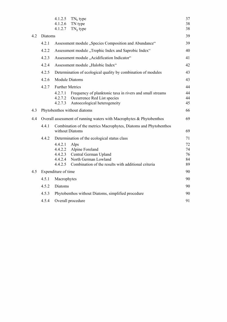
4.1.2.5 TNk type 37 4.1.2.6 TN type 38 4.1.2.7 TNg type 38

4.2 Diatoms 39 4.2.1 Assessment module „Species Composition and Abundance“ 39 4.2.2 Assessment module „Trophic Index and Saprobic Index“ 40 4.2.3 Assessment module „Acidification Indicator“ 41 4.2.4 Assessment module „Halobic Index“ 42 4.2.5 Determination of ecological quality by combination of modules 43 4.2.6 Module Diatoms 43 4.2.7 Further Metrics 44

4.2.7.1 Frequency of planktonic taxa in rivers and small streams 44 4.2.7.2 Occurrence Red List species 44 4.2.7.3 Autoecological heterogeneity 45

4.3 Phytobenthos without diatoms 66

4.4 Overall assessment of running waters with Macrophytes & Phytobenthos 69 4.4.1 Combination of the metrics Macrophytes, Diatoms and Phytobenthos

without Diatoms 69 4.4.2 Determination of the ecological status class 71

4.4.2.1 Alps 72 4.4.2.2 Alpine Foreland 74 4.4.2.3 Central German Upland 76 4.4.2.4 North German Lowland 84 4.4.2.5 Combination of the results with additional criteria 89

4.5 Expenditure of time 90 4.5.1 Macrophytes 90 4.5.2 Diatoms 90 4.5.3 Phytobenthos without Diatoms, simplified procedure 90 4.5.4 Overall procedure 91

Janurary 2006

1

1 Preliminary remarks

The assessment procedures described in the following were developed and tested as part of a research program and are based on a limited number of sampling sites. For this purpose, organisms were assigned to different indication groups. The resulting species lists were completed by referring to literature. These species lists might be incomplete or faulty, but this can only be verified in the course of further application. It is of high relevance that a potential adjustment of the classification is centralised and is exclusively carried out by those in charge of this project in cooperation with specialists. Ideally the project team in cooperation with the BAVARIAN ENVIRONMENT AGENCY should be consulted.

Further information regarding this instruction protocol and how it was developed can be found in SCHAUMBURG et al. 2005.

January 2006

2

2 Sampling and determination of the macrophyte & phytobenthos biocoenosis

Sampling is carried out once a year in summer, the main growing season of macrophytes. The ideal mapping time for each biocoenosis (usually mid June until early September) must be determined for each type of water according to the conditions in the field. The entire benthic vegetation aspect of a sampling section is investigated. Macrophyte vegetation is mapped in the field; diatoms are sampled and are stored for preparation. Phytobenthos without Diatoms is macroscopically determined and samples are taken for microscopic analysis. If an assessment procedure could not be developed for each module of a certain type of running water, for the time being, it will be assessed by using the other modules.

The exact location of the sampling site should be marked on topographical maps of the scale 1:25 000 or 1:50 000, so that later easting and northing of the sampling sites can be determined. Ideally, the coordinates can be read directly from a GPS. In this case the exact starting point and endpoint of a sampling section should be noted as precisely as possible.

The first step of sampling is the exact determination of the sampling section. For this purpose the running water is investigated from the shore. A decision which site to pick for macrophyte mapping is made based on the criteria described in chapter 2.1.2, page 4. The field report to assess structural quality is filled in. If a survey of structural quality is already at hand, this step can be omitted. Within the macrophyte mapping section an area for phytobenthos sampling is determined (chapter 2.3.1, page 14). The diatom sampling site is determined according to the criteria described in chapter 2.2.2, page 6.

In order to be able to take largely undisturbed diatom samples, sampling is carried out prior to entering the site for the purpose of macrophyte and phytobenthos mapping. Subsequently phytobenthos without diatoms is investigated and then the macrophyte vegetation. All investigations and sampling procedures have to be carried out as carefully as possible. It must be tried not to destroy other groups of organisms.

Documentation of the sampling procedure and mapping procedure is an important basis for evaluation and interpretation of the results. The field protocols presented in the instruction protocol contain all information relevant to the procedure. The reiteration of the information regarding abiotic characteristics on all field protocols serves to guarantee an unambiguous attribution of the original data collected in the field. If different specialists work on different components, the additional information regarding the sampling site is available to all. If sampling of the entire benthic flora is carried out by only one specialist, it is not necessary to note the abiotic characteristics on each sheet. A field protocol can be used that only once requires the documentation of abiotic factors (appendix C, figure 16, figure 17).

Janurary 2006

3

2.1 Macrophytes

2.1.1 Mapping equipment

Italics: optional • Topographic maps of a scale 1:25 000 or 1: 50 000 • Field protocols • Copy of the instruction protocol • Field protocol for mapping structural quality (LÄNDER WORKING GROUP WATER 2000) • Instruction for mapping structural quality (LÄNDER WORKING GROUP WATER 2000) • Writing utensils • Wading pants • Extractable rake • Under water viewer • Camera and films • Freezer bags and clips • Cooler and cooling elements • Envelopes or paper collecting packets for moss samples • Determination literature (compare below) • Magnifier • (Portable) stereo microscope and accessories • Herbarium press and accessories • Safety equipment if necessary (e.g. life vest)

Determination literature (selection) • CASPER & KRAUSCH (1980, 1981) • KLAPP & OPITZ VON BOBERFELD (1990) • KRAUSCH (1996) • KRAUSE (1997) • OBERDORFER (1994) • ROTHMALER (1994a, 1994b) • SCHMEIL (1993)

Special literature for moss determination (selection) • BERTSCH (1959) • BURCK (1947) • DEMARET & CASTAGNE (1964) • FRAHM & FREY (1992) • FREY, FRAHM, FISCHER & LOBIN (1995) • LANDWEHR (1984) • MÜLLER (1957) • NEBEL & PHILIPPI (2000) • NEBEL & PHILIPPI (2001) • NYHOLM (1986) • NYHOLM (1993) • PAUL, MÖNKEMEYER & SCHIFFNER (1931) • SCHUSTER (1980) • SMITH (1992) • WELCH (1960)

January 2006

4

2.1.2 Determination of the sampling section

Mapping of macrophyte vegetation is carried out in the main growing season (mid June until mid September) along river sections that from an ecologic point of view can be considered homogenous. Above all, the investigated section should be homogenous regarding velocity of flow, shading and sediment conditions. Adjacent to a sampling section there should not be drastic changes in land use (e.g. forest/pasture). Moreover, there must be no inflows (e.g. tributaries, drainages) into the sampling section of the running water system. If the composition of macrophyte vegetation abruptly changes, the investigated area must be reduced. For sampling sites close to bridges or weirs it has to be seen that mapping is carried out in upstream direction of these modifications, i.e. outside of the direct area of influence. The maximum length of a mapping section is approximately 100 m or longer, if necessary.

2.1.3 How to fill in the field protocol

On page 1 of the standardised field protocol (appendix C, figure 9) the structural characteristics at the sampling site are recorded. Fields marked in grey are optional, i.e. they only need to be filled in, if a detailed mapping procedure is carried out (see above). Apart from general information, characteristic structural parameters, e.g. mean depth, water level, mean width and optionally also turbidity are recorded. Shading of the entire section is estimated according to

WÖRLEIN’S five degree scale (1992). Determination of the flow velocity is carried out according to the mapping and assessment procedure of structural quality of the BAVARIAN WATER

MANAGEMENT AGENCY (1995). Unusual features regarding colouration and odour of the water can be noted verbally. The substratum conditions at the sampling site are classified in 5% steps according to an eight point scale (distribution of grain size according to SCHACHTSCHABEL et al. 1992). In addition, reinforcements of the river bank and foreign substrata are noted. If, in case of large running waters, it is impossible to investigate the entire cross section, it is noted whether the entire running water was investigated or only the area along the shore. For each sampling site at least two photographs (e.g. upstream and downstream) should be taken. In addition unusual or striking features at the sampling site are noted as well as the length of the mapping section.

The macrophytes occurring in the mapping section are investigated by wading along the sampling section and inspecting it, if possible, in upstream direction. To evaluate the entire width of the running water one should wade in a zigzag pattern. An under water viewer or a comparable viewing aid is absolutely recommended. If a river section is deep and wading is impossible using a boat is possible, but not obligatory.

Stoneworts, mosses and vascular plants are recorded, which at mean water levels grow submerged or at least are rooted under water. As far as possible, species determination is carried out on site. If necessary, samples are taken and determined later. Characeae and phanerogams are best transported in labelled freezer bags which contain little water and which are kept in a cooler.

Janurary 2006

5

Moss samples are stored in paper collecting packets, the so called “moss capsules” for which a DIN A4 paper is folded in the following fashion (Figure 1). The lower third of the sheet is folded upwards (1), then approx. 2 cm of the left and right side are folded inwards (2, 3) in order to seal the edges. In the end, the upper third of the sheet is folded downwards to function as a cover (4). The moss samples can be dried in these - ideally pencil labelled - paper packets. For later determination they can be remoistened.

Figure 1: Folding a moss capsule

On the second page of the field protocol (appendix C, figure 10) the species and their abundances according to KOHLER (1978) are noted. In addition, it is noted whether plants are submerged or emerged. Optionally also vitality and sociability as well as details regarding the sediment of the macrophyte stand are noted and if herbarium samples were taken. If a species occurs in two growth forms, e.g. in a submerged and emerged form or on two very different substrata (e.g. stone or wood), the species is noted twice in the field report. In that case plant abundance is also noted twice. Furthermore, however, the total abundance of the taxon at a particular site is recorded. For general characterisation of a sampling site the dominant species growing along the shore should be briefly noted.

If a sampling section is very deep and/or very turbid, the plants are mapped by using an extractable rake (max. length = 3 m, width = 60 cm, spaces between tines approx. 2 cm). Deep and inaccessible running waters are investigated from the water’s edge by wading into the river as far as possible and carefully raking the bottom. Mapping by boat with the help of divers is another option. The type of mapping procedure must be noted in the field protocol. If it is only possible to sample directly along the shore, this must also be noted in the field protocol (page 1).

The current version of the field protocol can be downloaded from the internet. (http://www.bayern.de/lfw/technik/gkd/lmn/fliessgewaesser_seen/pilot/fpmfg.pdf).

If a current assessment of structural quality is not already available, an exact morphological description of the sampling sites regarding riverbed, shoreline and surrounding area can be provided by filling in the “Field report for mapping structural quality in accordance with the recommendations of the LAWA 1998” (LÄNDER WORKING GROUP WATER 2000, appendix C, figure 11 and figure 12).

January 2006

6

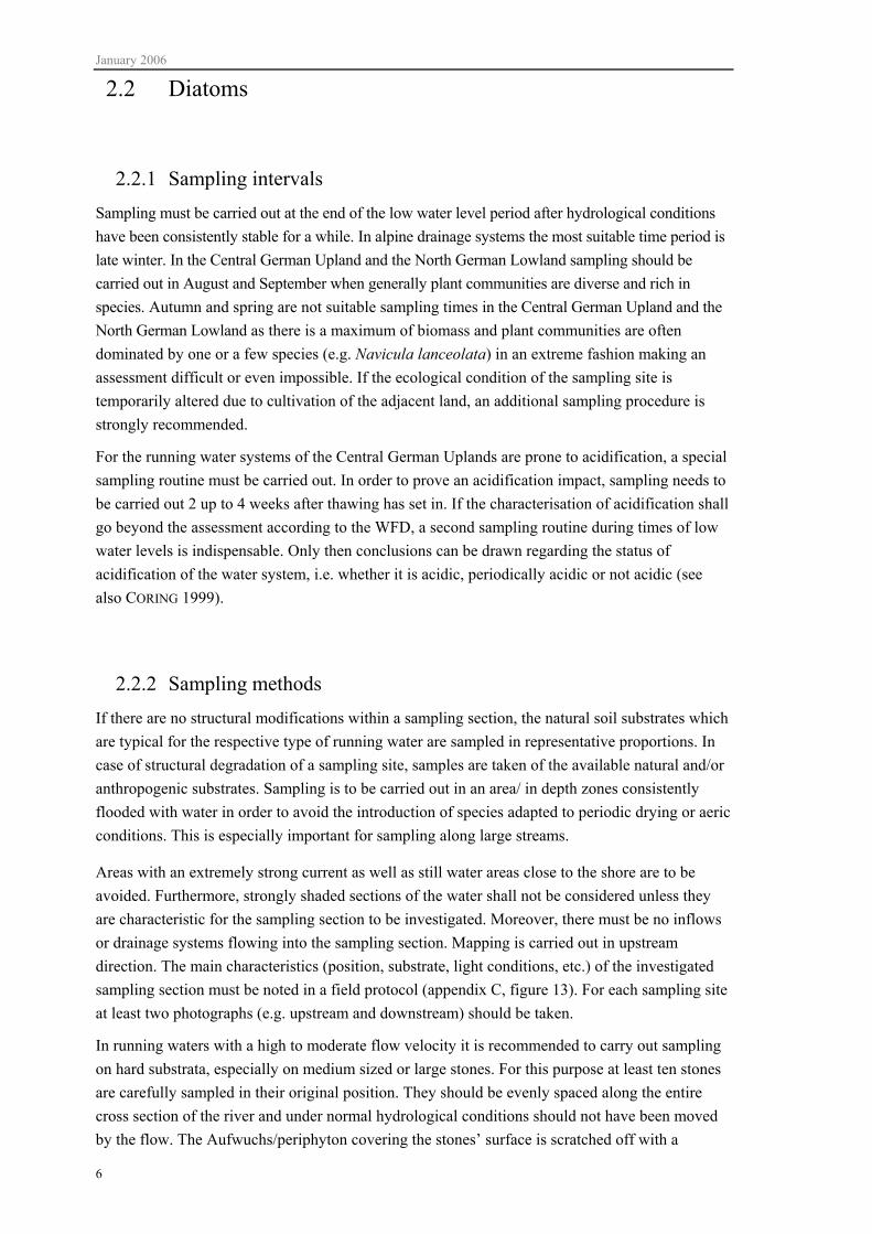
2.2 Diatoms

2.2.1 Sampling intervals Sampling must be carried out at the end of the low water level period after hydrological conditions have been consistently stable for a while. In alpine drainage systems the most suitable time period is late winter. In the Central German Upland and the North German Lowland sampling should be carried out in August and September when generally plant communities are diverse and rich in species. Autumn and spring are not suitable sampling times in the Central German Upland and the North German Lowland as there is a maximum of biomass and plant communities are often dominated by one or a few species (e.g. Navicula lanceolata) in an extreme fashion making an assessment difficult or even impossible. If the ecological condition of the sampling site is temporarily altered due to cultivation of the adjacent land, an additional sampling procedure is strongly recommended.

For the running water systems of the Central German Uplands are prone to acidification, a special sampling routine must be carried out. In order to prove an acidification impact, sampling needs to be carried out 2 up to 4 weeks after thawing has set in. If the characterisation of acidification shall go beyond the assessment according to the WFD, a second sampling routine during times of low water levels is indispensable. Only then conclusions can be drawn regarding the status of acidification of the water system, i.e. whether it is acidic, periodically acidic or not acidic (see also CORING 1999).

2.2.2 Sampling methods If there are no structural modifications within a sampling section, the natural soil substrates which are typical for the respective type of running water are sampled in representative proportions. In case of structural degradation of a sampling site, samples are taken of the available natural and/or anthropogenic substrates. Sampling is to be carried out in an area/ in depth zones consistently flooded with water in order to avoid the introduction of species adapted to periodic drying or aeric conditions. This is especially important for sampling along large streams.

Areas with an extremely strong current as well as still water areas close to the shore are to be avoided. Furthermore, strongly shaded sections of the water shall not be considered unless they are characteristic for the sampling section to be investigated. Moreover, there must be no inflows or drainage systems flowing into the sampling section. Mapping is carried out in upstream direction. The main characteristics (position, substrate, light conditions, etc.) of the investigated sampling section must be noted in a field protocol (appendix C, figure 13). For each sampling site at least two photographs (e.g. upstream and downstream) should be taken.

In running waters with a high to moderate flow velocity it is recommended to carry out sampling on hard substrata, especially on medium sized or large stones. For this purpose at least ten stones are carefully sampled in their original position. They should be evenly spaced along the entire cross section of the river and under normal hydrological conditions should not have been moved by the flow. The Aufwuchs/periphyton covering the stones’ surface is scratched off with a

Janurary 2006

7

toothbrush1, tea spoon, spatula or similar device and is transferred into a labelled wide neck sampling container with a volume of at least 100 ml. Toothbrushes can only be used once in order to avoid potential contamination. In different types of water the percentage of colonisation with diatoms can vary considerably. In some locations the Aufwuchs cannot macroscopically be seen, but can be felt by touching the surface of the substrate. In any case a large amount should be sampled. After the sample has settled at least 5 ml of diatomaceous sediment should remain.

In order to assess different types of stress by using indices, KELLY et al. (1998) recommend the sampling of vertically exposed hard substrata, e.g. bridge piers or moorings, for slowly running waters. For investigations aiming to assess biocoenoses specific for certain types of water systems this procedure only rarely is the method of choice. The substratum naturally occurring in these water systems is to be preferred which in general consists of sand, gravel or fine sediment. In areas where wading is possible, the upper millimetres of the bottom substratum are carefully lifted off with a spoon. In areas with a higher velocity of flow this method might not work, as often the sample on the spoon is swept away by the flow. Due to a lack of experience, presently no standardised sampling procedure for such sampling sites is on hand. It still needs to be developed. In order to gain the upper levels of substratum sediment cores or sediment grabs can be useful. It should also be verified, if pipetting off the water is the method of choice. In waters of Lower Saxony shovels have turned out to be useful tools when lifting off the upper layers of sediment while standing on the shore.

The sampling of deep Low Land running waters sometimes turns out to be a problem for steep shores can make it difficult or impossible to enter the sampling site. When choosing sampling sites accessibility must be given priority, even if one has to select a less representative site.

The samples are preserved in the field or at the latest in the evening after sampling by adding formaldehyde of a final concentration of 1% to 4%. Until further processing the samples are to be kept in a storage room.

2.2.3 Sampling equipment for running waters

• Topographical maps of a scale 1:25.000 or 1:50.000 • GPS if available • Field protocol • Copy of the instruction protocol • Writing utensils • Wading pants • Wide neck bottles or vials • Water proof marker to label sampling containers • Toothbrush1, tea spoon, spatula or something similar • Formaldehyde solution • Camera equipment • Safety equipment

1 Disposable toothbrushes can be ordered via specialised dental trade, e.g. John-Dental- und Medizintechnik GmbH: Disposable toothbrush without toothpaste, Tel.: 033762/42977, E-Mail: [email protected].

January 2006

8

2.2.4 Preparation

2.2.4.1 Preparation equipment

Chemicals • Acetic acid 25% p.a. • Sulphuric acid 95-97% for analysis • Potassium nitrate for analysis • Formaldehyde

Additional equipment • Hood • Hot plate • Safety clothing (lab coat, goggles, safety gloves, chemical proof lab gloves, if necessary) • Beakers (100 ml or larger) • Weighing glass with diameter corresponding to beakers • Beaker tongs • Magnetic stirrer • Mortar and pistil to pulverize potassium nitrate, if necessary • Spatula • Small plastic sieve with diameter corresponding to diameter of beaker • Universal indicator paper for pH determination • Aqua dest. • Wash bottle

2.2.4.2 Acid treatment

In order to determine diatoms to the species level, shape and structure of the siliceous valves must be focused on. Exact determination requires permanently mounted specimens. Especially species with small frustules can only safely be determined in a purified sample after removal of organic substance and other unwanted organic components. There are different procedures for preparation of the sampling material depending on the nature of the sample. A description of the most common preparation techniques is presented by KRAMMER & LANGE-BERTALOT (1986). For preparation of periphytic (Aufwuchs) substratum samples (stone, gravel, mud), which might contain a high percentage of organic material not containing diatoms, oxidation by strong acids (especially sulphuric acid) has turned out to be a useful method.

2.2.4.3 Treatment with acetic acid

If the material is from calcareous waters, the sample is initially boiled in acetic acid in order to prevent the formation of gypsum in the subsequent treatment with sulphuric acid. If the water content of the sample is high, the sample is allowed to sediment for 24 hours and then it is carefully decanted. Alternatively the sample can be heated until most of the water is evaporated. Prior to acid treatment a portion of the sampling material must be taken as a retain sample. The remaining sample is then mixed by shaking and approximately 20 ml of the sampling material are transferred into a 100 ml beaker to which 20–40 ml diluted acetic acid (25 %) are added. If the

Janurary 2006

9

sample is strongly calcareous, prior to heating the acetic acid has to be added little by little to keep foam formation at a minimum. The sample is covered with a weighing glass and by boiling it for 30 minutes with a magnetic stirrer, the carbonates are dissolved and the protoplasm and protoplasmic threads are dissolved and frustules are separated from the substratum. If the sand content of the sample is high, it is likely that the beaker starts moving on the hotplate and that its position needs to be corrected. This can best be accomplished by using beaker tongs. When rinsing the beaker tongs in or with tap water, one must make sure not to accidentally transfer any sampling material from one sample to the next. Magnetic stirrers must also be cleaned between the different boiling routines.

After boiling the sample is allowed to cool off. If present, subsequently large remainders are sieved off with a small kitchen sieve and the beaker is filled with tap water. In order to largely remove sand, gravel or smaller stones, which might be present, the solution is vigorously stirred and allowed to sediment for a minute so that the diatom containing supernatant can be decanted. In the following, the sample is carefully decanted several times until approximately one third of the volume is left and is rinsed with tap water. A four fold washing and decanting routine has proven to be adequate. However, the sedimentation time between washings should not be less than 24 hours. Alternatively the sample can be centrifuged between washings in a table centrifuge for approximately 10 minutes at maximally 2 000 rpm and the supernatant (approximately two thirds) can be decanted or removed with a jet pump. This procedure allows a quick preparation, but is labour intensive and might cause long diatom frustules to break.

2.2.4.4 Treatment with sulphuric acid

The water content of the sample is reduced by decanting, then approximately 20 to 30 ml concentrated sulphuric acid are added and the sample is boiled. In 20 minute intervals a dash of potassium nitrate is added with a spatula until the sample loses its colour or gets a yellow tint. If the content of organic material is low, a few dashes of potassium nitrate are sufficient, but if the content is high, the boiling procedure can take up to eight hours. After changing colour, the sample needs to remain on the hot plate for another 20 minutes. After the sample has cooled off and the diatoms have settled they form a white to greyish sediment. Subsequently samples are washed until neutrality (indicator paper!) is reached. When adding water for the first time after boiling, one has to exercise extreme cautious as this can cause a strong reaction. Experience has shown that the washing routine should be carried out approximately eight times. The last washing of the sample should be carried out with distilled water. The purified sample is mixed by shaking the beaker and is transferred into a labelled vial (for labelling compare labelling of the microscope slide). The vials are to be stored in a storage room for documentation.

Carry out all boiling procedures described under an effective hood. Exercise caution and adhere to all work safety rules. Protective clothing and eye protection are mandatory.

January 2006

10

2.2.5 Preparation of permanently mounted specimen

2.2.5.1 Materials

• Microscope slides • Cover slip (recommended are round cover slips with18 mm diameter) • Round tip tweezers or special tweezers to handle cover slips • Vials (10 ml recommended) • Naphrax2 • Storage system for mounted specimen • Labels Cover slips must be cleaned prior to adding the diatom suspension. A quick immersion into a highly concentrated solution with dishwashing detergent has proven suitable to remove fat and to reduce surface tension. Afterwards the suspension in the vial is mixed by shaking and immediately after a small amount is transferred with a clean pipette on to a cover slip. In order to reduce convection, the drop of sampling solution should be kept flat. If a suspension is highly concentrated, it often is necessary to dilute it in a weighing glass with distilled water. The degree of dilution depends on the density of valves desired for the preparation and on the presence of remaining organic components. Problems are often caused by a high content of mineralic components (loam and clay particles) which in a vial optically are impossible to differentiate from diatoms. For this reason it is useful to prepare different dilutions of the sample.

The ideal density of valves is reached, if after checking one or more complete transects under a 1000 fold magnification the required amount of 400 valves (compare below) is reached. The explanation is a partial demixing of diatom frustules caused by convection in the drop of sample solution on the cover slip. In case of strong convection flows, small frustules can be concentrated in the middle of the cover slip, whereas a high percentage of big and heavier frustules is concentrated along the edges. This phenomenon is compensated by counting complete transects.

In order to avoid contamination, one has to absolutely make sure to rinse used pipettes under running water prior to handling a new sample. After air drying the diatom sample overnight, a drop of Naphrax2 is added to a labelled, fat free microscope slide and using tweezers the cover slip is carefully placed on top of the sample coated side facing down. In order to evaporate the solvent, the sample is heated over the small flame of a Bunsen burner until bubbles can be observed for about 5 seconds. Afterwards it is immediately placed on a vibration free, smooth surface until it has cooled off. Napharax2 contains toluene that evaporates during heating and therefore must be handled with great care. Alternatively the evaporation of toluene can be carried out on a hot plate. Afterwards tweezers should be used to check if the cover slip strongly sticks to the microscope slide. If not, the procedure has to be repeated.

Immediately after completion of this procedure the sample can be evaluated under the light microscope and, if kept under appropriate conditions, it can be stored for decades. It is of essential importance to have a storage or archiving system and to precisely label microscope slides.

Janurary 2006

11

The information on the slides should contain the name of the sampling site or running water, position of the site (if available easting and northing). Furthermore, the sampled substratum, the date and, if available, any coded information which can be linked to other sources of data should be added.

After mounting of the permanent samples the diatom suspension remaining in the vial is preserved by adding two to three drops of a 30 percent formaldehyde solution. In order to keep the sample from drying out, five to ten drops of glycerine are added prior to placing the sample into storage.

2.2.6 Microscopic evaluation

In order to obtain a representative distribution, 400 diatom objects are determined to the species level with a 1000 fold up to 1200 fold magnification in microscopic slides prepared as described above. Partially the differentiation of varieties might be necessary (compare chapter 4.2.1). During counting the valve views as well as the girdle views are to be considered. When dealing with representatives of the Naviculaceae it is often impossible to tell from a valve view whether one is looking at single valves or entire frustules. Therefore during evaluation no difference is made between single or double valves, but one focuses on counting diatom objects. If valves of a frustule were not separated during preparation they are counted as a unit. Girdles which are impossible to determine must be characterized on the genus level and, if possible, must be grouped and categorized according to their size. After completion of microscopic analysis these diatom objects are attributed to the species they most likely represent according to the percentages with which these species occur. Fragments are only considered, if their size exceeds that of half a valve. Frequencies of species are presented as percentages. The results of diatom counting are to be documented along with data processing numbers according to MAUCH et al. (2003) in Excel or Access files or in specific databases.

When counting diatoms only benthic as well as benthic/planktonic taxa are considered. Taxa which are exclusively planktonic are not considered. For reliable literature regarding the life of centric taxa is not in all cases available and sometimes is even contradictory, with the exception of Melosira varians, Centrales are not considered during counting. The same is true for pennate taxa which are exclusively planktonic, e.g. Asterionella formosa, Fragilaria crotonensis, Nitzschia acicularis. Details regarding the different life forms can be found in KRAMMER & LANGE-BERTALOT (1986-1991).

The four volumes of KRAMMER & LANGE-BERTALOT (1986–1991) are the standard determination literature. In case of some genera or taxa it should be completed by the supplementary volumes and revisions of individual genera published since 1993 by the following authors: KRAMMER

(2000), LANGE-BERTALOT (1993, 2001), LANGE-BERTALOT & MOSER (1994), LANGE-BERTALOT & METZELTIN (1996). In the water systems of the North German Lowland influenced by saline conditions additionally the work of WITKOWSKI & LANGE-BERTALOT (2000) must be taken into account. However, the revision of the genus Cymbella by KRAMMER (2000, 2002, 2003) can be neglected.

January 2006

12

2.2.7 Criteria for a reliable assessment and evaluation Samples are not suitable for assessment if the percentage of diatom objects that cannot be determined (sp., spp.) and/or cannot unambiguously be determined (cf., aff.) exceeds 5 %.

If, even after the best possible isolation of the sampling material there is still only a small amount of diatoms, this suggests that sampling was not carried out correctly or that the time of sampling was not suitable (Chapter 2.2.1). A minimum of 50 objects in a cover slip (18 mm diameter) transect at 1000 fold magnification are suggested as a criterion for evaluation. If one surmises that the sample cannot be evaluated, the density of diatoms must be tested by counting a transect. Experience has shown that despite careful operating, the portion of samples that cannot be evaluated can amount to 3 %.

Another exclusion criterion is a large number of aerophilic diatoms in the sample. This can occur if a recently flooded section is sampled in which the water level still rises. If the portion of aerophilic taxa (Table 1) exceeds 5%, most likely there is a strong aeric influence dominating or at least strongly influencing the assessment. Additional information regarding the aerophilic character of the taxa can be found in KRAMMER & LANGE-BERTALOT (1986–1991).

Janurary 2006

13

Table 1: Aerophilic taxa according to LANGE-BERTALOT (1996) and HILDEBRAND (1991)

DV-Nr. Name Author6247 Achnanthes coarctata (BREBISSON) GRUNOW 6286 Amphora montana KRASSKE 6287 Amphora normannii RABENHORST 16692 Denticula creticola (OESTRUP) LANGE-BERTALOT & KRAMMER 6344 Diploneis minuta PETERSEN 16264 Hantzschia abundans LANGE-BERTALOT 6084 Hantzschia amphioxys (EHRENBERG) GRUNOW 6802 Hantzschia elongata (HANTZSCH) GRUNOW 16267 Hantzschia graciosa LANGE-BERTALOT 16271 Hantzschia subrupestris LANGE-BERTALOT 16276 Hantzschia vivacior LANGE-BERTALOT 6805 Melosira dickiei (THWAITES) KUETZING 6449 Navicula aerophila KRASSKE 6458 Navicula brekkaensis PETERSEN 6467 Navicula cohnii (HILSE) LANGE-BERTALOT 6858 Navicula contenta GRUNOW 16003 Navicula egregia HUSTEDT 6489 Navicula gallica var. perpusilla (GRUNOW) LANGE-BERTALOT 6492 Navicula gibbula CLEVE 6504 Navicula insociabilis KRASSKE 6028 Navicula mutica KUETZING 16020 Navicula nivalis EHRENBERG 16021 Navicula nivaloides BOCK 16022 Navicula nolensoides BOCK 16025 Navicula paramutica BOCK 16026 Navicula parsura HUSTEDT 6013 Navicula pelliculosa (BREBISSON) HILSE 6528 Navicula pseudonivalis BOCK 16360 Navicula pusilla var. incognita (KRASSKE) LANGE-BERTALOT 16366 Navicula saxophila BOCK 16036 Navicula subadnata HUSTEDT 16375 Navicula suecorum var. dismutica (HUSTEDT) LANGE-BERTALOT 6569 Neidium minutissimum KRASSKE 6574 Nitzschia aerophila HUSTEDT 16393 Nitzschia bacillariaeformis HUSTEDT 6921 Nitzschia debilis ARNOTT 16407 Nitzschia epithemoides var. disputata (CARTER) LANGE-BERTALOT 16050 Nitzschia harderi HUSTEDT 16053 Nitzschia modesta HUSTEDT 6614 Nitzschia terrestris (PETERSEN) HUSTEDT 16453 Nitzschia valdestriata ALEEM & HUSTEDT 16460 Orthoseira dendroteres (EHRENBERG) CRAWFORD 16060 Orthoseira roeseana (RABENHORST) O'MEARA 6148 Pinnularia borealis EHRENBERG 6635 Pinnularia frauenbergiana REICHARDT 6645 Pinnularia krookii (GRUNOW) CLEVE 16473 Pinnularia lagerstedtii (CLEVE) CLEVE-EULER 6654 Pinnularia obscura KRASSKE 6225 Simonsenia delognei (GRUNOW) LANGE-BERTALOT 6679 Stauroneis agrestis PETERSEN 16081 Stauroneis borrichii (PETERSEN) LUND 16558 Stauroneis gracillima HUSTEDT 16083 Stauroneis lundii HUSTEDT 16084 Stauroneis muriella LUND 6685 Stauroneis obtusa LAGERSTEDT 16095 Surirella terricola LANGE-BERTALOT & ALLES

January 2006

14

2.3 Phytobenthos without Diatoms In order to minimize the required input of time, in addition to the complete and detailed assessment procedure alternatively a simplified procedure was developed. The detailed procedure is based on a survey as complete as possible of all detectable phytobenthos algae including microscopic forms in all sampling sections to be assessed according to the biocomponent Macrophytes and Phytobenthos. The simplified procedure is limited to phytobenthos that can macroscopically be detected. In some type of sampling sites carrying out the simplified procedure results in a significantly reduced number of reliable assessments (SCHAUMBURG et al. 2005).

In the following, the simplified procedure is described. Differences to the detailed version are specifically pointed out so that the description at hand can be used to carry out both procedures. Partly directions were taken from the draft of the CEN standard for sampling of phytobenthos in shallow running waters (CEN/TC 230/WG 2/TG 3/N87).

2.3.1 Sampling

2.3.1.1 Phytobenthos sampling equipment

• Safety equipment • Topographic maps of a scale 1:25 000 or 1:50 000 or GPS • Camera • Wading pants or waders • Viewing aid • Rubber gloves • Magnifier • Sometimes helpful: rake, pliers or similar grabbing instruments • White plastic dish, if necessary, (2 to 3 l) for sorting material • Spoon, tweezers, spatula • Scalpel or knife (stainless steel) • Pipettes • Clean screw cap glasses, small (15-20 ml) and large • Petri dishes (plastic) • Freezer bags of different sizes • Ready made water proof labels or duct tape and a water proof marker for labelling samples • Cooler with cooling elements or ventilator • Large bucket to transport larger samples of substratum • Acidic Lugol’s solution or neutralised formaldehyde • Water proof lab book or field report and pencil • Plastic containers for storage The assessment procedure is based on a single sampling procedure per year. Sampling should be carried out when the water level is very low and after a phase of comparatively stable water level. After a period of flooding one should wait at least 4 weeks until sampling. For small rivers the sampling section to be investigated should have a length of 20 m, for larger streams approximately 50 m. In order to guarantee reproducibility of the investigation, the position of the sampling site should be noted exactly on a topographic map of a scale 1:25 000 or 1:50 000, so

Janurary 2006

15

that later easting and northing of the sampling sites can be determined. Ideally coordinates can be read directly from a GPS. Photographs should be made in upstream and downstream direction of the sampling site for documentation. All data pertaining to the sampling section and the sub samples taken are noted in the field protocol (Appendix C, Figure 14).

For both simplified as well as detailed analysis sampling is carried out according to the procedure of Multi-Habitat-Sampling (MHS).

It is the goal of the sampling procedure to report as completely as possible covers of benthic algae and growth forms that can macroscopically be detected. For this purpose all habitats within a sampling section should be observed. They mainly differ in substrate, velocity of flow, depth and light conditions. During sampling one walks along the sampling section and then – as far as possible with waders - one walks through it. The river bed is examined with an underwater viewer. In sections which are impossible to wade through or can only partially be examined sampling is only representative to a certain degree. In such cases tools like a rake or a pair of pliers with long handles can be useful (chapter “Phytobenthos sampling equipment”, page 14). Several samples are taken in one sampling site reflecting the different aspects of the sampling site. These samples are called “sub samples”.

Note: Sampling is identical for the detailed and simplified procedure.

In a first step all growth forms and covers that can macroscopically be detected are noted as separate sub samples in the field protocol. Colour as well as growth form are described as exactly as possible and possibly photographs are taken for documentation. Some striking growth forms are listed in the following.

• Fine floating filaments or tufts (e.g. Zygnema, Stigeoclonium) • Green filamentous tufts on stones or plants (e.g. Cladophora, Oedogonium, Microspora) • Green patches (e.g. Vaucheria) • Green or red filaments on stones in areas of wave action (e.g. Ulothrix, Bangia) • Light green, mucilaginous floating filaments (e.g. Spirogyra, Mougeotia) • Light green or yellowish netlike floating forms (e.g. Hydrodictyon) • Green to brown coarse wiry filaments (e.g. Lemanea) • Small ruby coloured, blue, violet or blackish tufts on stones (e.g. Audouinella, Chantransia) • Black stains, pustules or wart like structures on stones (e.g. Chamaesiphon) Covers of different colour

(blue-black, turquoise, dark blue, grey, black, greenish, golden) (e.g. Phormidium, Phaeodermatium) • Widespread ruby coloured or blackish crusts (e.g. Hildenbrandia), also calcified (e.g. Homoeothrix

crustacea) • Gelatinous colonies or thalli (e.g. Tetraspora, Hydrurus, Batrachospermum, Nostoc) • Leave shaped or tube shaped thalli (e.g. Enteromorpha) • Leathery or felty mats (e.g. Phormidium) • Attached spheroidal or hemispheric colonies, also calcified (e.g. Rivularia) • Epiphytic algae (e.g. Chamaesiphon, Coleochaete) • Metaphytic algae (growing in between aquatic plants) (e.g. Closterium, Chroococcus) • Algae living on sand, mud or silt (e.g. Euglena, Closterium)

January 2006

16

A small amount is sampled of filamentous forms, of thalli or gelatinous colonies and is transferred into an appropriate container (small glass vial). If stones with a striking cover are detected, it is advisable to take along the representative stones. They are sampled and packaged into suitable plastic bags (freezer bags). In this fashion later the different samples can individually be examined under the stereo microscope. If, in contrast, periphyton is scratched off the stones, a mixture of epilithic algae is the result which makes microscopic determination more difficult. Covers on sand, mud and clay or other substrata can be sampled with a spoon, tweezers or a pipette. In some cases it is possible to sample sediment by turning a petri dish upside down on the substrate and then pushing a spatula underneath.

These sub samples are enumerated starting with the number 2 (the number 1 is needed for the overall assessment, compare below) and are unambiguously labelled (number of sampling section, name of running water, position, date, number of sub sample). In the field protocol for each sub sample the percentage cover (percentage of the entire sampling section) is noted. Additionally the mean thickness of the periphyton cover in mm or cm can be noted.

The second step is to take samples of the substrata present at the site:

Immoveable substrata (boulder, bedrock, parts of trees, trees, roots) smaller pieces are broken off or cover is scratched off with a scalpel. These samples are packaged in plastic bags (freezer bags) and along with some water are transferred into small glass vials with a 15-20 ml volume.

Moveable hard substrata (stones of different sizes, smaller pieces of wood) are sampled and transferred into small plastic bags (freezer bags).

Plant substratum (mosses, macro algae, vascular plants, matting of roots) small tufts are taken and in a plastic bag with some river water are thoroughly squeezed. A portion containing a good amount of sampling material is transferred into a glass vial. A mixed sample consisting of different substrata from different locations of the sampling site.

In case of striking filamentous or floating forms small parts are transferred into a glass container along with some water. It is useful to carefully, but thoroughly clean off accumulations of detritus and mud off the sampled algae.

Fine sediments (sand, mud, fine particulate organic material, loam) can be sampled with a spoon, tweezers or a pipette. In some cases it is possible to turn a petri dish upside down on the sediment and catch the sediment by slipping a spatula underneath the dish. Fine sediments are only sampled if an algal cover is macroscopically striking.

Overall at least 5 sub samples should be taken to obtain reliable results. Especially macroscopically striking covers and growth forms must be investigated. Moreover stony material should be sampled and a crushed sample of plant substrate should be created.

Janurary 2006

17

2.3.2 Transport, preservation, storage and shipment of samples

Materials

• Fixative: for recipe compare appendix B • Transport: cooler and cooling elements • Short term storage (2-3 days): refrigerator • Long term storage of stones: freezer (ca. –20°C) If analysis of the samples can be carried out immediately after sampling, the freshly taken samples are transported to the lab in a cooler for analysis. Liquid samples are kept in the refrigerator (5-8 C°) with lids slightly ajar in order to allow gas exchange. The samples should be exposed to light on a daily basis. Hard substrates can be kept in the refrigerator for 2 to 3 days.

If microscopic evaluation cannot be carried out within this time, the samples must be preserved and stored (fixative compare appendix B).

If possible, liquid samples are preserved immediately with a few drops of acidic Lugol’s solution. Generally 5-10 drops are sufficient for a sample of 15-20 ml. Samples with a high content of organic matter (e.g. high density of algae, sand, mud, loam) need a higher concentration of Lugol’s solution (visual inspection: colour similar to that of Cognac). Samples preserved in this fashion should be stored in a cool, dark and well aerated room for no longer than a year (if status of preservation is regularly controlled). Neutralised formaldehyde can also be used for preservation. Then samples can be stored for a longer period of time.

For hard substrates cryopreservation is the method of choice, i.e. until analysis they are kept in a freezer. Frequent freezing and thawing of the material, however, is to be avoided.

A combination of preservation and conservation procedures has turned out to be best for the samples. Lugol’s solution alters the colours of the sampling material but preserves cell organelles. Cryopreservation preserves the colours, but does have an impact on cell organelles. For determination of taxa, however, all these characteristics are of importance.

If the samples are sent to an expert for microscopic evaluation, the preserved liquid samples must be packed in a shatter-proof fashion. Stones can be packaged in a thermo bag for transporting frozen goods (super market) along with cold cooling elements. The samples should reach their destination within a day.

January 2006

18

2.3.3 Microscopic analysis and documentation

2.3.3.1 Materials

• White plastic dishes • Petri dishes (diameter ca. 10 and 20 cm) • Scalpel • Tweezers in different sizes • Brushes • Preparation needles • Pasteur pipettes • Camera with macro mode (digital or conventional films) • Stereo microscope (magnification 6,7 up to 40-fold) with external light source and camera equipment

(digital conventional films) • Compound light microscope with stage and 40- to 1000-fold magnification. An eyepiece micrometer

for measuring cells is required. For documentation of the taxa found camera equipment is essential (digital or conventional films). For determination of organisms optical contrasting methods, e.g. interference contrast are very helpful

• Microscope slides and cover slips • Cellulose wipes • Tap water • Lens paper and special lens cleaning paper and cleaning agent • Glycerine and clear nail polish (for preparation of permanent specimen) • Storage device with lid for permanently mounted specimen • Dye to proof the existence of storage compounds etc. (compare determination literature) • Clean, small glass bottles (15-20 ml) with screw cap for storage purposes • Labels or duct tape and markers to label samples • Acidic Lugol’s solution or neutralised formaldehyde for preservation

2.3.3.2 Microscopy

The evaluation of samples is carried out with a stereo microscope (magnification 6,7 fold to 40 fold) as well as with a microscope (magnification 40 fold to 1000 fold). For documentation of the species detected (compare below) microscope camera equipment is essential. A camera for the stereo microscope is desirable.

It is the goal of microscopic analysis to determine, if possible, the taxa of the representative sub samples to the species level. According to our present knowledge we cannot recommend to limit the analysis to the indicator species mentioned. To be able to settle any taxonomic questions, each taxon should be photographed.

Preserved liquid samples usually can be analysed without any pre-treatment. If the sampling material turns out to be inhomogeneous, it is recommended to first observe the sampling material in a petri dish (if necessary add tap water) under the stereo microscope at low magnification. If different growth forms can be found, they should be documented and afterwards be examined under the microscope one by one. Please exercise caution when handling samples preserved with formalin.

Janurary 2006

19

Frozen stones must first be thawed. If different covers or kinds of growth are found (e.g. during inspection under the stereo microscope), they must be analysed separately.

Parts of coloured covers, stains, pustules, wart like structures or crusts are removed with a scalpel or a brush and then are applied to a microscope slide with a little water.

Filaments, tufts or patches are partly taken of the substratum with tweezers and are then applied to a microscope slide with a little water. It can be necessary for determination to include holdfasts or any other structures that serve to adhere to the substratum into the analysis. This is also true for leathery felty mats. In this way also epiphytic algae are documented.

For a more detailed analysis, gelatinous colonies (e.g. Nostoc) can be squeezed onto the microscope slide with the cover slip (squash preparation).

Rhodophytes with a thallus as well as other algae classes with leaf- or tube shaped thalli must be preserved for determination so that reproductive organs and other morphological characteristics can be recognized. For documentation we recommend glycerine based permanently mounted specimen.

Epipsamnic algae must be applied to the microscope slide with a small amount of water and as little sand, silt and mud as possible.

Liquid samples with metaphytic algae can directly be applied to the microscope slide with a pipette.

For each sub sample a microscopy protocol is filled in (example is given in appendix C, figure 15). All taxa which are microscopically common or massive are listed. The abundance of each taxon is recorded according to the descriptions in Table 2. In contrast to the complete analysis of phytobenthos, for the simplified analysis only those taxa are recorded which are microscopically massive (abundance 3). Species which are microscopically rare (abundance 1) are not considered.

Table 2: Estimating abundance

Abundance Description

3 macroscopically rare, barely recognizable (note in field protocol: “solitary specimen“ or 5 % coverage) or

microscopically massive

2 microscopically common

1 microscopically rare

Note: If possible, for the detailed procedure all taxa present in a sample are determined to the species level and are also noted if their abundance is low. Microscopically rare corresponds to abundance 1.

Regarding labour intensity there are the following recommendations for the simplified analysis (Table 3):

3 to 5 cover slips should be prepared for samples taken off boulder, gravel, sand and mud as well as off floating material.

• For samples taken off boulders, gravel, sand and mud as well as floating material 3 to 5 cover slips should be prepared

• For samples of stones and plant material more than 5 cover slips might be necessary.

January 2006

20

• 30 to 60 minutes should be spent on the microscopic analysis of stony substrata, approximately 30 minutes on plant substrata and approximately 15 minutes on all other types of substratum.

Table 3: Recommendations regarding the required input of time and labour to process sub samples

Substratum Maximum amount of cover slips

Mean maximum input of time

Sand, mud 3 - 5 15 min. Fine gravel 3 - 5 15 min.

Coarse gravel, stones possibly more than 5 60 min. Boulder 3 - 5 15 min.

Floating material 3 - 5 15 min. Mosses and macrophytes

squash preparation possibly more than 5 30 min.

After investigation the samples should be preserved and kept in storage. If it turns out that during the simplified analysis not enough indicative taxa were found to obtain a reliable assessment, a detailed analysis can easily be carried out by examining further samples under the microscope. There is no need to carry out the sampling procedure again.

Note: Recommendations regarding the input of time for the detailed procedure (Table 4):

Table 4: Recommendations regarding the required input of time and labour to process sub samples

Substratum Max imum number of cov er slips

Max imum input of time

Sand, mud max. 5 30 min.

Fine gravel max. 5 30 min.

Coarse gravel, stones Possibly more than 5 90 min.

Boulder max. 5 30 min.

Floating material max. 5 30 min.

Mosses and macrophytes squash preparation

Possibly more than 5 60 min.

Determination literature

Excluding diatoms and Charales, there is a considerable amount of phytobenthos determination literature wich is consistently being refined. At present we recommend the literature listed below for determination of benthic algae. The most important literature is marked in grey.

Comprehensive literature for different algal groups

• BOURRELLY, P. (1968) • BOURRELLY, P. (1972) • BOURRELLY, P. (1970) • ENTWISLE,T.J., SONNEMANN, J.A., LEWIS, S.H. (1997) • JOHN, D.M.; WHITTON, B.A.; BROOK, A.J. (Hrsg.; 2002) • KANN, E. (1978) • LINNE VON BERG, K.-H. & MELKONIAN, M. (2004) • PANKOW, H. (1990): • SIMONS, J.; LOKHORST, G.M.; VAN BEEM, A.P. (1999) • WEHR, J.D. & SHEATH, R.G. (2003) Nostocophyceae

• ANAGNOSTIDIS, K. & KOMÁREK, J. (1988a, b)

Janurary 2006

21

• GEITLER, L. (1932) • KANN, E. & KOMÁREK, J. (1970) • KOMÁREK, J. (1999) • KOMÁREK, J. & ANAGNOSTIDIS, K. (1989) • KOMÁREK J. & ANAGNOSTIDIS, K. (1998) • KOMÁREK, J. ANAGNOSTIDES K. (2005) • KOMÁREK, J. & KANN, E. (1973) • KOMÁREK, J. & KOVÁCIK, L. (1987) • MOLLENHAUER, D., BENGTSSON, R. & LINDSTRØM, E.-A. (1999) • STARMACH, K. (1966) Bangiophyceae / Florideophyceae / Fucophyceae

• COMPÈRE, P. (1991) • ELORANTA, P. & KWANDRANS, J. (1996) • FRIEDRICH, G. (1966) • KUMANO, S. (2002) • LEUKART, P. & KNAPPE, J. (1995) • NECCHI, O.; SHEATH, R.G.; COLE K.M. (1993a) • NECCHI, O.; SHEATH, R.G.; COLE K.M. (1993b) • NECCHI, O. & ZUCCHI, M.R. (1993) • RIETH, A. (1979) • SHEATH, R.G.; WHITTICK, A.; COLE K.M. (1994) • SHEATH, R.G. & VIS, M.L. (1995) • STARMACH, K. (1977) • VIS, M.L.; SHEATH, R.G.; ENTWISLE, T.J. (1995) • WEHR, J.D. & STEIN, J.R. (1985) Or comrehensive literature pertaining to different groups Chrysophyceae/Synurophyceae

• KRISTIANSEN, J. & PREISIG, H.R. (2001) • STARMACH, K. (1985) Cryptophyceae / Dinophyceae

• FOTT, B. (1968) • POPOVSKY, J. & PFIESTER, L.A. (1990) Euglenophyceae

• HUBER-PESTALOZZI, G. (1955) • KUSEL-FETZMANN, E. (2002) • WOŁOWSKI, K. (1998) • WOŁOWSKI, K. & HINDÁK, F. (2005) Tribophyceae

• CHRISTENSEN, T.A. (1970) • ETTL, H. (1978) • RIETH, A. (1980) Chlorophyceae / Trebouxiophyceae / Ulvophyceae / Tetrasporales/

• LOCKHORST, G.H. (1999) • ETTL, H. (1983) • ETTL, H. & GÄRTNER, G. (1988) • FOTT, B. (1972) • HUBER-PESTALOZZI, G. (1961) • KOMÁREK, J. & FOTT, B. (1983) • MROZINSKA, T. (1985)

January 2006

22

• PRINTZ, H. (1964) • STARMACH, K. (1972) • HOEK, C. (1963) Charales excl. Characeae

• COESEL, P.M. (1982) • COESEL, P.M. (1983) • COESEL, P.M. (1985) • COESEL, P.M. (1991) • COESEL, P.M. (1994) • COESEL, P.M. (1997) • CROASDALE, H. & FLINT, E.A. (1986) • CROASDALE, H. & FLINT, E.A. (1988) • CROASDALE, H.; FLINT, E.A.; RACINE, M.M. (1994) • FÖRSTER, K. (1982) • KADLUBOWSKA, J.Z. (1984) • LENZENWEGER, R. (1996) • LENZENWEGER, R. (1997) • LENZENWEGER, R. (1999) • LENZENWEGER, R. (2003) • RŮŽIČKA, J. (1977) • RŮŽIČKA, J. (1981)

2.3.3.3 Summarisation and processing of data

After microscopic analysis the taxa lists of the individual sub reports are combined in one report. It is referred to as sub report 1 and lists all taxa which during microscopic analysis were assigned an abundance of 3 (microscopically massive). Simultaneously for each sub sample the degrees of coverage of the different coatings noted in the field protocol need to be considered for a final determination of abundance. The final abundances of the taxa are attributed according to the description in Table 5.

Table 5: Estimating abundance – simplified procedure

Abundance Description

5 Massive, covering more than 1/3 of the river bed (degree of coverage > 33%)

4 Frequent, but covering less than 1/3 of the river bed (degree of coverage 5-33%)

3 Macroscopically rare, barely noticeable (note in field protocol:

„solitary finding“ or „5% coverage“) or microscopically massive

After microscopic analysis for each sampling procedure the results are available in form of a species list (including abundances for each species). Based on these species lists the sampling section can be evaluated for the time of sampling.

Janurary 2006

23

Note: For the detailed procedure for each taxon the highest abundance is noted which was attributed during microscopic analysis. If in at least three sub reports a taxon had the same abundance, for the overall assessment abundance is upgraded by one step. This means that a taxon which in four sub reports was microscopically rare (abundance 1) is attributed an abundance of 2 for the overall assessment. For those taxa which were microscopically massive for the final assessment of abundances the abundances or degrees of cover and the different growth forms noted in the field protocols must be considered. In this fashion the final abundances of the taxa can be determined according to Table 6.

Table 6: Estimating abundances – detailed procedure

Abundance Description5 massiv e, cov ering more than 1/3 of the riv er bed

(degree of cov erage > 33 %)4 common, but cov ering less than 1/3 of the riv er bed

degree of cov erage 5–33 %)3 macroscopically rare, barely recognizable (note in

field protocol: „solitary specimen“ or „5 % degree of ov erage

cov erage or microscopically massiv e2 microscopically common1 microscopically rare

January 2006

24

3 Determination of the type of running water

For application of the assessment procedure the sampled water system must correctly be assigned to the Macrophyte and Phytobenthos biocoenotic types. The LAWA type map which is nationwide in effect can serve as an aid for type determination, but not as the sole basis. Any relevant additional information must be taken into consideration. Additional simplifications for type attribution are presently being verified.

If the parameters relevant for determination of the macrophyte type and phytobenthos type are strongly influenced by anthropogenic factors, one should refer to values representing the sampling section in its original state (state of reference). This can pertain to parameters like depth, velocity of flow, width and also to acid capacity or water hardness. If modifications of this sort are noticed (e.g. backwaters, ramps) or known (e.g. potash mining in upper reaches, discharge of limed water from sewage treatment plants into siliceous areas), their impact (e.g. altered velocity of flow, increased hardness) must be ignored for type determination. In some cases helpful conclusion can be drawn from the attribution of the measuring point to the LAWA typology.

The LAWA typology according to SOMMERHÄUSER & POTTGIESSER (2004) describes different geochemical types (of low basicity and high basicity or siliceous and calcareous) in their state of reference. If a running water is attributed to the macrophyte and phytobenthos typology based on the LAWA typology of running waters this differentiation must be kept in mind.

If for the macrophytes the MRK type is determined and the acid capacity or total hardness measured are only slightly above the limit of 1,4 mmol/l, and if the sampling site can be characterised by a siliceous geology, for the macrophytes also the results of the siliceous type MRS (which is analogue to the calcareous type) must be calculated and the results must be discussed.

If no measurements of acid capacity and total hardness are available, in the case of MRS or MRK types, the result of calculation must thoroughly be checked for plausibility. If necessary, the analogous type must also be determined and both results must be discussed. Regarding the differentiation siliceous/calcareous or low basicity/high basicity, the same is true for type attribution of the subcomponent Phytobenthos without Diatoms.

If type attribution is unclear, always the analogous type must be determined and its ecological condition must be calculated. The situation can be unclear due to missing information, the location of the sampling site or if chemical, physical parameters are difficult to classify. Both results must be discussed.

To make attribution of macrophyte types easier their characteristics were summarised and can be looked up in the appendix pages 95 to 107.

Problems upon attributing the biocoenotic diatom type can occur in the transition zone of ecoregions and if the bedrock in the catchment area is heterogeneous. The latter is especially true for water systems with a catchment area showing siliceous as well as calcareous influence and

Janurary 2006

25

which are differently assessed in the module “Trophic Index” (SCHAUMBURG et al. 2005). In this case typefication must be carried out based on the dominant geology of the catchment area (siliceous or calcareous) and must be discussed correspondingly. A total hardness or acid capacity of 1,4 mmol/l can be used as an auxiliary criterion. However, a heterogeneous geology does not affect the module „Species Composition and Abundance“ as in this case siliceous as well as calcareous reference species can be referred to (compare chapter 4.2.1)

January 2006

26

Alps

As due to a lack of data for the Alps ecoregion no assessment procedure for the module „Phytobenthos without Diatoms“ could be developed, the assessment is carried out according to the WFD with the modules „Macrophytes“ and „Diatoms“. The biocoenotic water types of the Alps ecoregion are determined according to Tale 7 and Table 8.

Tale 7: Determination key for finding macrophyte types in the ecoregion Alps.

Macrophytes

1a Depth class = 1 ............................................................................................................. Type MRK 1b Depth class ≥ 2 ............................................................................................................. 2

2a Mean width ≥ 40m ....................................................................................................... 5 2b Mean width < 40m ....................................................................................................... 3

3a Velocity of flow > III...................................................................................................... Type MRK 3b Velocity of flow ≤ III...................................................................................................... 4

4a Influence of groundwater.............................................................................................. Type MPG 4b No influence of groundwater ........................................................................................ Type MP

5a Velocity of flow > III...................................................................................................... Type MRK 5b Velocity of flow ≤ III...................................................................................................... 6

6a Depth class = 3 ............................................................................................................. Type Mg 6b Depth class < 3 ............................................................................................................. 4

Table 8: Determination key for finding diatom types in the ecoregion Alps. LAWA type according to SOMMERHÄUSER & POTTGIESSER (2004)

Diatoms

LAWA-Type 1.1 .............................................................................................................................. D 1.1

LAWA-Type 1.2 .............................................................................................................................. D 1.2

Alpine Foreland The running water of the tertiary hill region, river terraces and older moraines in the Alpine Foreland are considered slightly calcareous, but also siliceous. Those of the younger moraines are considered mostly calcareous (BRIEM 2003). This difference is reflected in the diatom assemblages. In the investigation at hand, however, no macrophyte societies with a siliceous character were found in the Alpine Foreland. This means that theoretically conditions typical for the MRS type of macrophytes can be found, but that this is very unlikely. If these conditions are the result of type determination, all parameters should be verified for correctness and the result should only be accepted under reservation. It is impossible that diatoms characterise a calcareous water system while macrophytes of the same sampling section characterise a siliceous water system.

Due to a lack of data for the running water systems of the Alpine Foreland, no assessment procedure could be developed for the module “Phytobenthos without Diatoms“. As a consequence the assessment according to the WFD is carried out with the module “Macrophytes“ and the module “Diatoms“.

The biocoenotic water types of the Alpine Foreland are determined according to Table 9 and Table 10.

Janurary 2006

27

Table 9: Key for type determination in the Alpine Foreland

Macrophytes

1a Depth class = 1 ............................................................................................................. 2 1b Depth class ≥ 2 ............................................................................................................. 3

2a Maximum value of total hardness or median of acid capacity 4,3 < 1,4 mmol/l ............ Type MRS 2b Maximum value of total hardness and median of acid capacity 4,3 ≥ 1,4 mmol/l .......... Type MRK


4a Velocity of flow > III ..................................................................................................... 2 4b Velocity of flow ≤ III...................................................................................................... 5


6a Velocity of flow > III ..................................................................................................... 2 6b Velocity of flow ≤ III...................................................................................................... 7

7a Depth class = 3 ............................................................................................................. Type Mg 7b Depth class < 3 ............................................................................................................. 5

Table 10: Key for diatom type determination in the Alpine Foreland ecoregion. LAWA-Type according to SOMMERHÄUSER & POTTGIESSER (2004)

Diatoms

LAWA-Type 1.1 .............................................................................................................................. D 1.1

LAWA-Type 1.2 .............................................................................................................................. D 1.2

LAWA-Type 2 ................................................................................................................................ D 2

LAWA-Type 3 ................................................................................................................................ D 3

LAWA-Type 11 and Alpine Foreland ecoregion ................................................................................. D 3



LAWA-Type 4 ................................................................................................................................ D 4

Central German Upland Areas with variegated sandstone and volcanoes, which are very common in the Central German Upland as well as areas with gneiss, granite and slate have a siliceous character just like the waters running through them. However, calcareous water can enter a catchment area consisting of calcareous and siliceous areas so that the siliceous character is largely lost. For the diatom type is strongly linked to the dominating geochemical situation and the macrophyte type is linked to total hardness and acid capacity, the combination of a siliceous diatom type and a calcareous macrophyte or phytobenthos type is definitely possible. In such a case it needs to be thoroughly verified, if the increased values of hardness and acid capacity, which were the basis for attribution to the calcareous type, are not due to, for example, the inflow of industrial sewage or limed water. If this is the case, assessment must be based on the siliceous type.

Only in very rare cases combinations of siliceous macrophyte and phytobenthos types along with a calcareous diatom type can be observed. If this is the result of type determination, all relevant parameters must be checked again for correctness. If necessary, measurements must be taken again or another sampling site must be chosen.

The biocoenotic water types of the Central German Upland are determined according to, Table 11, Table 12 and Table 13.

January 2006

28

Table 11: Key for macrophyte type determination in the Central German Upland

Macrophytes

1a Depth class = 1 ............................................................................................................. 2 1b Depth class ≥ 2 ............................................................................................................. 3

2a Maximum value of total hardness or median of acid capacity 4,3 < 1,4 mmol/l ............ Type MRS 2b Maximum value of total hardness and median of acid capacity 4,3 ≥ 1,4 mmol/l .......... Type MRK


4a Velocity of flow > III...................................................................................................... 2 4b Velocity of flow ≤ III...................................................................................................... 5


6a Velocity of flow > III...................................................................................................... 2 6b Velocity of flow ≤ III...................................................................................................... 7

7a Depth class = 3 ............................................................................................................. Type Mg 7bc Depth class < 3 ............................................................................................................. 5

Table 12: Key for diatom type determination in the ecoregion Central German Upland. LAWA type according to

SOMMERHÄUSER & POTTGIESSER (2004)

Diatoms

LAWA-Type 5 excl. Subtype 5.2 (volcanic rock) ............................................................................. D 5

LAWA-Type 5.1 ................................................................................................................................ D 5

LAWA-Type 11 and Central German Upland ecoregion..................................................................... D 5

LAWA-Type 5.2 ................................................................................................................................ D 6

LAWA-Type 9 ................................................................................................................................ D 7

LAWA-Type 6 D 8.1

LAWA-Type 19 and Central German Upland ecoregion................................................................... D 8.1

LAWA-Type 9.1 and loess-, keuper- and cretaceous regions excl. shell limestone,............................ D 8.2 Jura-, Malm-,Lias-, Dogger-and other calcareous regions

LAWA-Type 7 .............................................................................................................................. D 9.1

LAWA-Type 9.1 and shell limestone-, Jura-, Malm-, Lias-, Dogger-and other ................................. D 9.2 calcareous regions excl. loess-, keuper- and cretaceous regions

LAWA-Type 9.2 ............................................................................................................................. D 10.1

LAWA-Type 10 ............................................................................................................................. D 10.2

Table 13: Key for phytobenthos type determination in the Central German Upland ecoregion. LAWA-Type according to SOMMERHÄUSER & POTTGIESSER (2004)

Phytobenthos without Diatoms

LAWA-Type 5 ............................................................................................................................. MG_sil

LAWA-Type 5.1 ............................................................................................................................. MG_sil

LAWA-Type 5.2 ............................................................................................................................. MG_sil

LAWA-Type 9 ............................................................................................................................. MG_sil

LAWA-Type 6 ........................................................................................................................... MG_carb

LAWA-Type 7 ........................................................................................................................... MG_carb

LAWA-Type 9.1 ........................................................................................................................... MG_carb

LAWA-Type 9.2 ........................................................................................................................... MG_carb

LAWA-Type 10 ........................................................................................................................... MG_carb

LAWA-Type 19 and Central German Upland ecoregion................................................................ MG_carb

Janurary 2006

29

North German Lowland

The biocoenotic water types in the North German Lowland ecoregion are determined according to Table 14, Table 15and Table 16. The terms “type of low basicity” and “type of high basicity”, “low basicity” and “high basicity” or “siliceous” and “calcareous” type correspond to the terms siliceous and calcareous used in the summarised characteristics of the different types of running waters in Germany (POTTGIESSER und SOMMERHÄUSER 2004).

Table 14: Key for type determination in the North German Lowland ecoregion.

Macrophytes

1a Mean width > 30 m ...................................................................................................... Type TNg 1b Mean width < 30 m ...................................................................................................... 2

2a Velocity of flow > III ..................................................................................................... Type TR 2b Velocity of flow ≤ III...................................................................................................... 3

3a Velocity of flow = III ..................................................................................................... 4 3b Velocity of flow < III ..................................................................................................... 5

4a Depth class = 1 ............................................................................................................. Type TR 4b Depth class ≥ 2 ............................................................................................................. 5

5a Mean width ≥ 5 m ........................................................................................................ TN 5b Mean width < 5 m ........................................................................................................ 6

6a Depth class = lll ............................................................................................................. TN 6a Depth class = ll.............................................................................................................. TNk

Table 15: Key for diatom type determination in the North German Lowland ecoregion. LAWA-type according to SOMMERHÄUSER & POTTGIESSER (2004).

Diatoms

LAWA-Type 11 and North German Lowland ecoregion, type of low basicity.....................................D 11.1

LAWA-Type 14 and siliceous type ....................................................................................................D 11.1

LAWA-Type 16 and siliceous type .....................................................................................................D 11.1

LAWA-Type 12 and North German Lowland ecoregion, type of low basicity, ...................................D 11.2 catchment area < 1.000 km²

LAWA-Type 11 and North German Lowland, type of high basicity ...................................................D 12.1

LAWA-Type 14 and calcareous type..................................................................................................D 12.1

LAWA-Type 16 and calcareous type..................................................................................................D 12.1

LAWA-Type 19 and North German Lowland ecoregion.....................................................................D 12.1

LAWA-Type 15 and catchment area < 1.000 km², excl. loess regions ...............................................D 12.2

LAWA-Type 17 and catchment area < 1.000 km² ............................................................................D 12.2

LAWA-Type 12 and catchment area < 1.000 km², ...........................................................................D 12.2 Ecoregion North German Lowland, type of high basicity

LAWA-Type 15 and catchment area > 1.000 km², loess regions excluded ........................................D 13.1

LAWA-Type 17 and catchment area > 1.000 km² ............................................................................D 13.1

LAWA-Type 12 and catchment area > 1.000 km², North German Lowland ecoregion, .....................D 13.1 type of high basicity

LAWA-Type 20 ………………………………………………………………………………………………………………D 13.2

January 2006

30

Table 16: Key for phytobenthos type determination in the North German Lowland ecoregion. LAWA Type according to SOMMERHÄUSER & POTTGIESSER (2004)

Phytobenthos

LAWA-Type 11 and North German Lowland ecoregion, type of low basicity................................ NT_sil/org

LAWA-Type 12 and North German Lowland ecoregion, type of low basicity ............................... NT_sil/org

LAWA-Type 14 and siliceous type ............................................................................................... NT_sil/org

LAWA-Type 16 and siliceous type ................................................................................................ NT_sil/org

LAWA-Type 11 and North German Lowland ecoregion, type of high basicity.................................. NT_cal

LAWA-Type 12 and North German Lowland ecoregion, type of high basicity.................................. NT_cal

LAWA-Type 14 and calcareous type ................................................................................................NT_ cal

LAWA-Type 15 ...............................................................................................................................NT_ cal

LAWA-Type 16 and calcareous type ................................................................................................NT_ cal

LAWA-Type 17 ...............................................................................................................................NT_ cal

LAWA-Type 18 ...............................................................................................................................NT_ cal

LAWA-Type 19 ...............................................................................................................................NT_ cal

LAWA-Type 20 ...............................................................................................................................NT_ cal

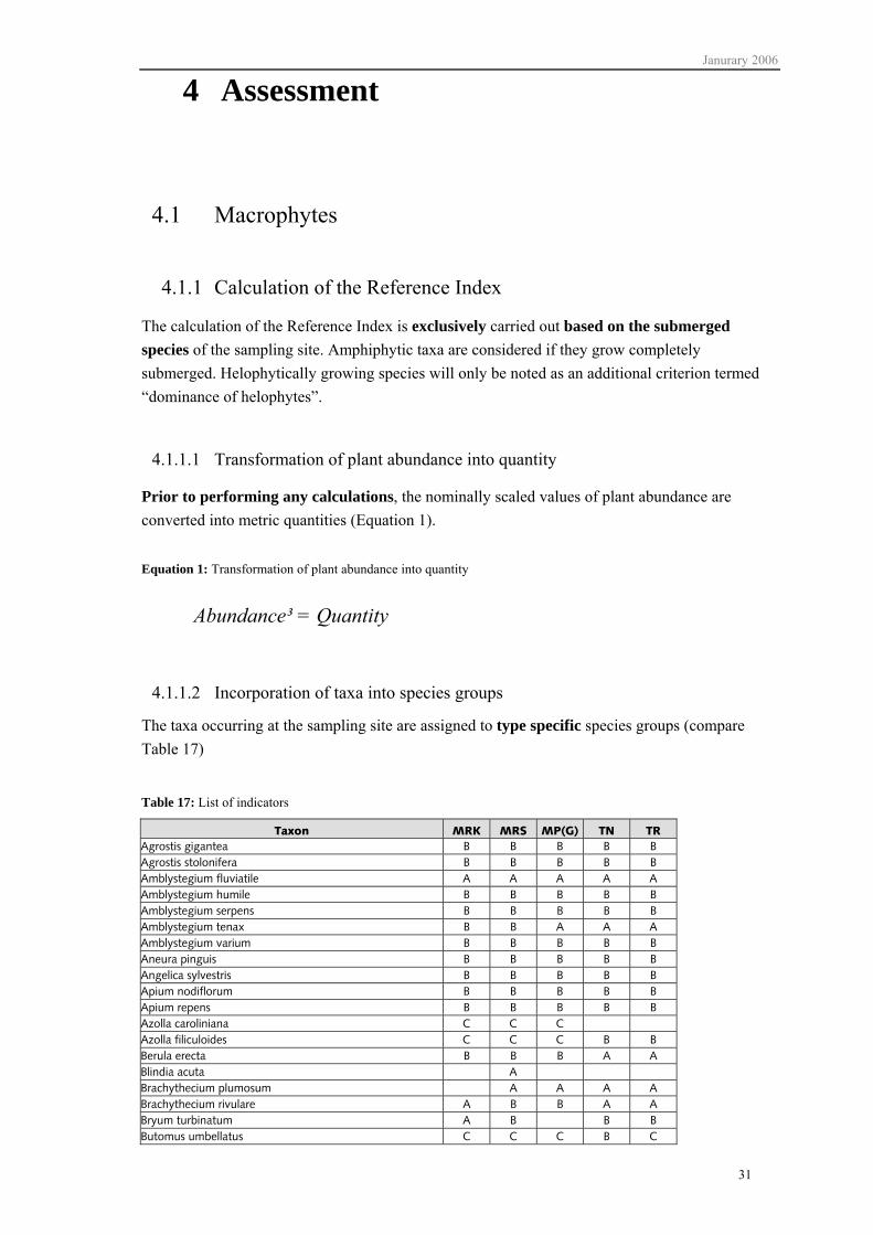
Janurary 2006

31

4 Assessment

4.1 Macrophytes

4.1.1 Calculation of the Reference Index

The calculation of the Reference Index is exclusively carried out based on the submerged species of the sampling site. Amphiphytic taxa are considered if they grow completely submerged. Helophytically growing species will only be noted as an additional criterion termed “dominance of helophytes”.

4.1.1.1 Transformation of plant abundance into quantity

Prior to performing any calculations, the nominally scaled values of plant abundance are converted into metric quantities (Equation 1).

Equation 1: Transformation of plant abundance into quantity

Abundance³ = Quantity

4.1.1.2 Incorporation of taxa into species groups

The taxa occurring at the sampling site are assigned to type specific species groups (compare Table 17)

Table 17: List of indicators

Taxon MRK MRS MP(G) TN TR Agrostis gigantea B B B B B Agrostis stolonifera B B B B B Amblystegium fluviatile A A A A A Amblystegium humile B B B B B Amblystegium serpens B B B B B Amblystegium tenax B B A A A Amblystegium varium B B B B B Aneura pinguis B B B B B Angelica sylvestris B B B B B Apium nodiflorum B B B B B Apium repens B B B B B Azolla caroliniana C C C Azolla filiculoides C C C B B Berula erecta B B B A A Blindia acuta A Brachythecium plumosum A A A A Brachythecium rivulare A B B A A Bryum turbinatum A B B B Butomus umbellatus C C C B C

January 2006

32

Taxon MRK MRS MP(G) TN TR Calliergon cordifolium B B B B B Calliergon giganteum A B A A A Callitriche cophocarpa b b b b b Callitriche hamulata A A A A A Callitriche hermaphroditica b b b b b Callitriche obtusangula B B B B B Callitriche platycarpa B B B A A Callitriche stagnalis A A A A Cardamine amara B B B B B Ceratophyllum demersum C C C C C Ceratophyllum submersum C C Chara aspera A A A A Chara contraria A A A A Chara delicatula A A A A Chara globularis A A A A Chara hispida A A A A Chara intermedia A A A A Chara tomentosa A A A A Chara vulgaris A A A A Chiloscyphus pallescens A A A A A Chiloscyphus polyanthos A A A A Cinclidotus aquaticus A B B Cinclidotus danubicus A B A A A Cinclidotus fontinaloides A B A A A Cinclidotus riparius B B Conocephalum conicum A B B B A Cratoneuron filicinum A A A A A Dichodontium pellucidum A A A A A Drepanocladus aduncus A B B A A Drepanocladus sendtneri A B A A A Eleocharis acicularis A A A A Elodea canadensis C C C B C Elodea nuttallii C C C B C Equisetum fluviatile B A A Equisetum palustre B Eucladium verticillatum A B Fissidens adianthoides B B B B B Fissidens arnoldii A A A A Fissidens crassipes B B B A A Fissidens grandifrons A A Fissidens gymnandrus B B B Fissidens pusillus B B B B B Fissidens rivularis A A A A A Fissidens rufulus A A A A A Fontinalis antipyretica B B B B B Fontinalis hypnoides A A A A A Fontinalis squamosa A A A Galium palustre B B B B B Glyceria fluitans B B B B B Glyceria maxima B B B B B Groenlandia densa B A A B Hippuris vulgaris B B A A Hottonia palustris C B A Hydrocharis morsus-ranae C B B B Hydrocotyle vulgaris B B B Hygrohypnum duriusculum A A Hygrohypnum eugyrium A A Hygrohypnum luridum A B A A A Hygrohypnum ochraceum A V A A A Hymenostylium recurvirostre A A Hyocomium armoricum A V A Isolepis fluitans A A Juncus articulatus B B A B B Juncus bulbosus A A A Juncus subnodulosus A A Jungermannia atrovirens A A A

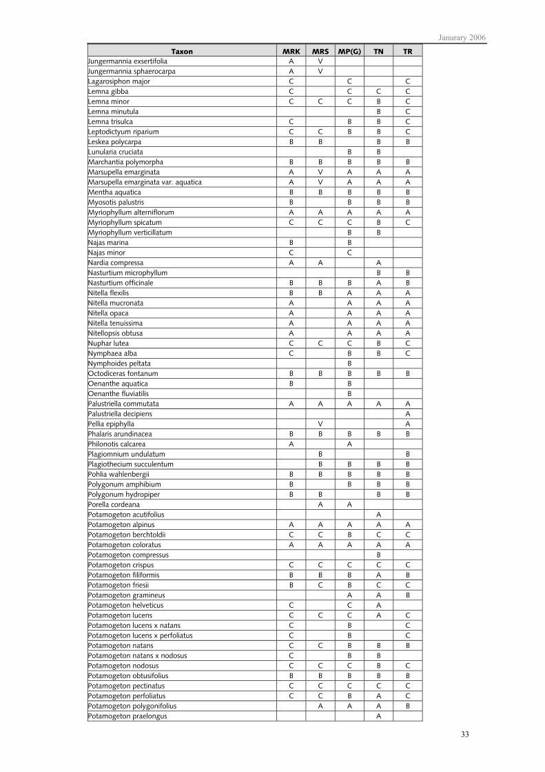
Janurary 2006

33

Taxon MRK MRS MP(G) TN TR Jungermannia exsertifolia A V Jungermannia sphaerocarpa A V Lagarosiphon major C C C Lemna gibba C C C C Lemna minor C C C B C Lemna minutula B C Lemna trisulca C B B C Leptodictyum riparium C C B B C Leskea polycarpa B B B B Lunularia cruciata B B Marchantia polymorpha B B B B B Marsupella emarginata A V A A A Marsupella emarginata var. aquatica A V A A A Mentha aquatica B B B B B Myosotis palustris B B B B Myriophyllum alterniflorum A A A A A Myriophyllum spicatum C C C B C Myriophyllum verticillatum B B Najas marina B B Najas minor C C Nardia compressa A A A Nasturtium microphyllum B B Nasturtium officinale B B B A B Nitella flexilis B B A A A Nitella mucronata A A A A Nitella opaca A A A A Nitella tenuissima A A A A Nitellopsis obtusa A A A A Nuphar lutea C C C B C Nymphaea alba C B B C Nymphoides peltata B Octodiceras fontanum B B B B B Oenanthe aquatica B B Oenanthe fluviatilis B Palustriella commutata A A A A A Palustriella decipiens A Pellia epiphylla V A Phalaris arundinacea B B B B B Philonotis calcarea A A Plagiomnium undulatum B B Plagiothecium succulentum B B B B Pohlia wahlenbergii B B B B B Polygonum amphibium B B B B Polygonum hydropiper B B B B Porella cordeana A A Potamogeton acutifolius A Potamogeton alpinus A A A A A Potamogeton berchtoldii C C B C C Potamogeton coloratus A A A A A Potamogeton compressus B Potamogeton crispus C C C C C Potamogeton filiformis B B B A B Potamogeton friesii B C B C C Potamogeton gramineus A A B Potamogeton helveticus C C A Potamogeton lucens C C C A C Potamogeton lucens x natans C B C Potamogeton lucens x perfoliatus C B C Potamogeton natans C C B B B Potamogeton natans x nodosus C B B Potamogeton nodosus C C C B C Potamogeton obtusifolius B B B B B Potamogeton pectinatus C C C C C Potamogeton perfoliatus C C B A C Potamogeton polygonifolius A A A B Potamogeton praelongus A

January 2006

34

Taxon MRK MRS MP(G) TN TR Potamogeton pusillus C C B C C Potamogeton trichoides C C C C C Potamogeton x nitens B A Potamogeton x zizii A Racomitrium aciculare A A A A Racomitrium aquaticum A Ranunculus aquatilis C B B Ranunculus circinatus B B B B C Ranunculus circinatus x trichophyllus B B Ranunculus flammula B A A Ranunculus fluitans B B B B A Ranunculus fluitans x trichophyllus B B B B A Ranunculus hederaceus A Ranunculus peltatus B B B B A Ranunculus penicillatus B B B B A Ranunculus trichophyllus B B B B Ranunculus x cookii B B Rhynchostegium alopecurioides A A A Rhynchostegium riparioides B B B B B Riccardia chamaedryfolia A A A Riccia fluitans B C B A C Riccia rhenana B C B A C Ricciocarpos natans A B C C Sagittaria latifolia C C C Sagittaria sagittifolia C C B C Scapania undulata V A A A Schistidium rivulare A A A Schoenoplectus lacustris B B B B B Scorpidium scorpioides A B A A Sparganium emersum C C C B C Sparganium erectum C C B C Sparganium minimum A C Sphagnum V A A A Spirodela polyrhiza C C C C C Stratiotes aloides A Thamnobryum alopecurum A B A A Tolypella glomerata A Tolypella prolifera A Trapa natans C C C Utricularia australis A A Utricularia ochroleuca A A Utricularia vulgaris A A Veronica anagallis-aquatica B B B B B Warnstorfia exannulata A A Warnstorfia fluitans A V A A A Zannichellia palustris C C C C C

4.1.1.3 Calculation of total quantities

The quantities of the different species calculated from the plant abundances of a sampling site are summed up separately for each indicator group and for all submerged species of a sampling site.

If in the course of new surveys species are found, which are not mentioned in the above species list, these species should not be considered for calculation of the index. If the number of unlisted (=non indicative) species is high, this most likely will falsify the calculated index. Consequently, if the percentage of non indicative species is ≥ 25 % of the total quantity, the index value cannot be considered reliable.

Janurary 2006

35

4.1.1.4 Criteria for a reliable assessment

Prerequisites for a reliable assessment

• the total quantity of all submerged indicator species in a sampling site must add up to a minimum of 26 and at the same time

• plant quantity of indicator species must exceed 75 %.

If the portion of listed macrophytes (indicator species) is below 75 %, the ecological status class determined on the basis of the index value cannot be considered reliable. In the overall assessment it can only serve to describe tendencies. If for a particular sampling site the minimum quantity is not reached, it must be verified whether this is the result of natural causes or macrophyte depopulation due to eutrophication. If the latter is the case, the respective sites must be assigned the ecological status class 5 (unreliable). Macrophyte degeneration must always be proven and must be backed up by structural, physical, chemical and biological investigations. Depopulation can be the result of trophic or saprobic stress, influence of herbicides, severe acidification, clearing or mowing of the site or introduction of herbivorous fish.

4.1.1.5 Calculation of the Reference Index

For the types MRK, MP(G), TR, TNk, TN as well as TNg the Reference Index is calculated according to the following formula (Equation 2):

Equation 2: Calculation of the Reference Index

100

1

11 ∗−

=

∑

∑∑

=

==g

CA

n

igi

n

iCi

n

iAi

Q

QQRI

RI = Reference Index QAi = Quantity of the i-th taxon of group A QCi = Quantity of the i-th taxon of group C Qgi = Quantity of the i-th taxon of all groups nA = Total number of taxa in group A nC = Total number of taxa in group C ng = Total number of taxa in all groups

For the MRS type the index calculation is carried out according to the following modified equation (Equation 3):

Equation 3: Calculation of the Reference Index for the MRS type

100

1

111 ∗−+

=

∑

∑∑∑

=

===

g

CVA

n

igi

n

iCi

n

iVi

n

iAi

Q

QQQRI

RI = Reference Index QAi = Quantity of the i-th taxon of group A QCi = Quantity of the i-th taxon of group C QVi = Quantity of the i-th taxon of group V Qgi = Quantity of the i-th taxon of all groups nA = Total number of taxa in group A nC = Total number of taxa in group C nV = Total number of taxa in group V ng = Total number of taxa in all groups

January 2006

36

4.1.2 Type specific characteristics of the assessment procedure Upon determination of the Reference Index the following type specific characteristics and prerequisites must be considered.

4.1.2.1 MRK type

No specific characteristics must be considered for the assessment of the macrophyte MRK type.

The Reference Index is calculated according to equation 2.

No additional criteria are calculated.

4.1.2.2 MRS type

The Reference Index is calculated according to equation 3.

In addition to macrophyte depopulation a depopulation of mosses must be verified.

The relevant additional criterion for the MRS type is acidification. If 100% of the mosses mapped in a certain section belong to the species group V, one is dealing with acidification. In such a case action needs to be taken at this sampling site.

4.1.2.3 MP(G) type

Type MPG is characterised by an increased influence of groundwater. In contrast to waters without groundwater influence, running waters fed by large amounts of groundwater have a smaller temperature amplitude, i.e. they are warmer in winter and cooler during the summer (POTT & REMY 2000). Generally, CO2-contents are relatively high (SCHWOERBEL 1994) and in their natural state they are oligotrophic.

The reference index for the MP type and the MPG type is calculated according to equation 2.

For the subtypes MP and MPG the additional criterion “minimum number of species”, must be considered along with the RI-value.

If the value of the RI exceeds –70 and if there are less than 4 submerged taxa the RI value is reduced by 30.

Janurary 2006

37

4.1.2.4 TR type

The reference index for the TR type is calculated according to equation 2.

The additional criterion „dominance of helophytes“ is considered valid, if the river bed of a section is covered throughout with dense populations of one or several of the following emerged species:

• Glyceria maxima • Phalaris arundinacea • Phragmites australis • Sagittaria sagittifolia • Sparganium emersum • Sparganium erectum • Urtica dioica Additional criteria for the TR type are:

• if RI ≥ 0 and dominance of helophytes, RI is reduced by 80

4.1.2.5 TNk type

The reference index for the TNk type is calculated according to equation 2.

For assessment of the additional criteria, the minimum number of species, the total quantity of the taxa Myriophyllum spicatum und Ranunculus ssp., dominance of helophytes and evenness must be considered.

The additional criterion „dominance of helophytes“ is considered valid, if the river bed of a section is covered throughout with dense populations of one or several of the following emerged species:

• Glyceria maxima • Phalaris arundinacea • Phragmites australis • Sagittaria sagittifolia • Sparganium emersum • Sparganium erectum • Urtica dioica The criterion „evenness“ (equation 5) is calculated based on the SHANNON & WEAVER(1949) diversity index (Equation 4).

Equation 4: Calculation of the Diversity Index

ln1∑=

⋅−=s

iiis NNH

Hs = Diversity Indey Ni = Quantity of the species i/Total quantity of all species s = Total number of taxa of the biocoenosis

Equation 5: Calculation of Evenness

ln sH

E s= E = Evenness Hs = SHANNON-WEAVER Diversity-Index s = Total number of species

January 2006

38

Additional criteria for the TNk type:

• if RI ≥ 0 and if there are less than five submerged taxa, the RI is reduced by 20 • if RI ≥ 0 and if evenness < 0,75, the RI is reduced by 30 • if RI ≥ 0 and if the total quantity of the taxa Myriophyllum spicatum and Ranunculus spp. >

60 % , the RI is reduced by 80 • if RI ≥ 0 and if there is a dominance of helophytes, the RI is reduced by 80 • if due to application of several criteria the RI falls < -100, a value of -100 will be stipulated

4.1.2.6 TN type

The Reference Index for the TN type is calculated according to equation 2.

For assessment of the additional criteria, the minimum number of species, the total quantity of the taxa Myriophyllum spicatum und Ranunculus ssp., dominance of helophytes and evenness must be considered.

The additional criterion „dominance of helophytes“ is considered valid, if the river bed of a section is completely covered with dense populations of one or several of the following emerged species:

• Glyceria maxima • Phalaris arundinacea • Phragmites australis • Sagittaria sagittifolia • Sparganium emersum • Sparganium erectum • Urtica dioica The criterion „evenness“ (equation 5) is calculated based on the SHANNON & WEAVER(1949) diversity index (Equation 4).

Additional criteria for the TN type:

• if RI ≥ 0 and if there are less than five submerged taxa, the RI is reduced by 20 • if RI ≥ 0 and if evenness < 0,75, the RI is reduced by 30 • if RI ≥ 0 and if the total quantity of the taxa Myriophyllum spicatum and Ranunculus spp. >

60 % , the RI is reduced by 80 • if RI ≥ 0 and if there is a dominance of helophytes, the RI is reduced by 80 • if due to application of several criteria the IR falls < -100, a value of -100 will be stipulated

4.1.2.7 TNg type

The Reference Index for the TNg type is calculated according to equation 2.

For assessment of the additional criteria, a minimum number of species, the total quantity of the taxa Myriophyllum spicatum und Ranunculus ssp. and evenness must be considered.

The criterion „evenness“ (equation 5) is calculated based on the SHANNON & WEAVER(1949) diversity index (Equation 4).

Janurary 2006

39

Additional criteria for the TNg type:

• if RI ≥ -40 and if there are less than 5 submerged taxa, the RI is reduced by 20 • if RI ≥ -40 and if evenness < 0,75 the RI is reduced by 30 • if RI ≥ -40 and if the total quantity of the taxa Myriophyllum spicatum and Ranunculus spp. >

60 % , the RI is reduced by 80 • if due to application of several criteria the IR falls < -100, a value of -100 will be stipulated

4.2 Diatoms

4.2.1 Assessment module „Species Composition and Abundance“

Assessment is carried out using the percentage of cumulated frequencies of the general reference species present at the sampling site. A distinction is made between general reference species and type specific reference species. General reference species are mostly oligotraphent and oligo-mesotraphent diatoms, but few euryoecious species are included. The majority of species has a clear geochemical preference and is either characteristic for siliceous or calcareous waters. A small number of species is indifferent towards basicity and can be found in both geochemical types of water. The total of 442 general reference species and their geochemical preference can be found in Table 24. The attribution of the siliceous and calcareous reference species to the different diatom types is summarised in Table 18.

The list of general reference species does not for all biocoenotic types reflect the actual species composition in high condition. Instead it provides an open “pool of species” with room for future additions to the reference species list of the different diatom types (also see Schaumburg et al. 2005) which in the course of increasing number of investigated waters in high ecological condition and increasing knowledge can be expected. In case of most species, the geochemical preferences are known and can be backed up by sufficient literature data. If presently the geochemical preference cannot accurately be specified, it can be looked up in Table 24. This is especially true for rare and/or taxa generally represented only by a few individuals.

January 2006

40

Table 18: Attribution of siliceous and calcareous reference species lists to the different diatom types. In this table subtypes are included in types of higher order.

Diatom type Siliceous reference species Calcareous reference species

1 x 2 x x 3 x 4 x x 5 x 6 x 7 x x 8 x 9 x

10 x x 11 x x 12 x x 13 x x

The so called type specific reference species (Table 23) are neither limited to the respective type, nor can they be considered to be reference species sensu strictu. These taxa are wide spread and in certain types of water even in good or high ecological condition can occur in great numbers.

Evaluation is carried out with the cumulated frequencies of the general and type specific reference species present at the sampling site. Cumulated frequencies between 76% and 100% characterise the high ecological condition, values between 51% and 75% represent a good ecological condition. Cumulated frequencies between 26% and 50% reflect a moderate ecological condition.

Additionally diversity is considered for evaluation of communities (SCHAUMBURG et al. 2005) for the water types of the Central German Upland and the North German Lowland (Type D 5 to D 13, including subtypes). If in a sampling site of this type the percentage of a type specific reference species exceeds a value of 40% (massive occurrence), the value 25 is subtracted from the sum of all reference species representing the sample. If in the diatom types of the Central German Upland and North German Lowland there is a massive occurrence of a general reference species it is advisable to verify the assessment by carrying out an additional sampling procedure.

4.2.2 Assessment module „Trophic Index and Saprobic Index“

The biocoenotic types of running waters 1 to 12 are assessed based on the Trophic Index according to ROTT et al. (1999) (Equation 6). The species specific parameters are listed in Table 25.

The Saprobic Index is the basis for the assessment of diatom type 13 (large rivers and streams of the North German Lowland) (Equation 7, Table 25).

The importance of the trophic or saprobic situation in the respective water types is explained in detail in SCHAUMBURG et al. 2005.

Janurary 2006

41

Equation 6: Calculation of the Trophic Index according to ROTT et al. (1999)

∑

∑

=

== n

iii

ii

n

ii

HG

HGTWTI

1

1

*

** TI : Trophic-Index TWi : Trophic value of the i-th species Gi : Weighting of species i Hi : Abundance of species i in percent

Equation 7: Calculation of the Saprobic Index according to ROTT et al. (1997)

∑

∑

=

== n

iii

ii

n

ii

HG

HGSWSI

1

1

*

** SI : Saprobic Index SWi : Saprobic value of species i Gi : Weighting of species i Hi : Abundance of species i in percent

4.2.3 Assessment module „Acidification Indicator“ For the rivers of the siliceous Central German Upland, especially for the waters of the variegated sandstone and the bedrock, the verification of acidification characteristics is indispensable and is carried out based on the occurrence of the quantitatively most important indicators of anthropogenic acidification (Table 19). These species are the typical components of undisturbed coenoses and therefore are listed as general reference species. However, if the ecological condition is high, there only is a small to moderate amount of these individuals. Only if acidification sets in, their portion rises and an extremely large number of individuals becomes a characteristic of permanently acidic plant communities.

Depending on the abundance of the acidification indicators the ecological status class determined based on the entire biocomponent Macrophytes & Phytobenthos is degraded according to Table 20 (compare chapter Combination of results with additional criteria, page 89). This simple way of incorporating degradation due to acidification is suitable for assessment according to the guidelines of the EC-WFD, but must not be regarded as a substitute of the existing procedures which exclusively serve to indicate acidification (e.g. CORING 1999). Application of this module is restricted to the siliceous waters of the Central German Upland.

Table 19: Indicators of anthropogenic acidification

DV-Nr Name Author

6253 Achnanthes helvetica (HUSTEDT) LANGE-BERTALOT

6975 Eunotia exigua (BREBISSON) RABENHORST

6214 Eunotia incisa GREGORY

6375 Eunotia rhomboidea HUSTEDT

6383 Eunotia tenella (GRUNOW) HUSTEDT

6513 Navicula mediocris KRASSKE

6543 Navicula soehrensis KRASSKE

16074 Pinnularia silvatica PETERSEN

6126 Pinnularia subcapitata var. subcapitata GREGORY

6665 Pinnularia subcapitata var. hilseana (JANISCH) O.MUELLER

January 2006

42

Table 20: Assessment module „Acidification Indicator“

Cumulated frequency of acidification indicators Degradation by

10% to 25% one ecological status class 26% to 50% two ecological status classes 51% to 99% three ecological status classes 100% four ecological status classes

4.2.4 Assessment module „Halobic Index“ In order to prove different degrees of salinisation in limnic water systems, the Halobic Index has proven its value. It is based on classifying species according to their occurrence in different zones of salinity (ZIEMANN 1971, 1999). Haloxenic or halophobic and halophilic taxa are differentiated. The group of halophilic taxa consists of halophilic, mesohalobic and polyhalobic forms, which altogether, without weighting, are considered for index calculation (Equation 8). The list of species is summarised in Table 26. Limnic (without oligohalobic preferences) taxa are not included in this list, but they are part of the sum in the denominator and thus are considered during calculation.

Halobic indices close to 0 are characteristic for typical soft waters, negative indices are characteristic for waters with low salinity which often are poor in electrolytes and/or are acidic. Values between +10 and +30 indicate and increased salt content. At a value of +30 one speaks of moderate salinisation and at values of +50 of severe salinisation. As summarised in Table 22, this is incorporated into an assessment module and follows the definition of ZIEMANN (1999). If the Halobic Index exceeds a value of 15 and if the assessment module Diatoms is applied exclusively and independent of an assessment according to the WFD, the ecological status class is degraded by one. For assessment according to the EU-Water Framework Directive by the means of the biocomponent Macrophytes & Phytobenthos, the metric „Salinisation“ only has an informative character and can, if necessary, be employed to plan restoration measures.

In waters affected by salinisation often mass occurrences of halophilic and/or mesohalobic species can be observed. If the halobic index is calculated based on percentages, indicative species of which only a small number of individuals were found are underrepresented. Therefore, abundances are used to calculate the Halobic Index (ZIEMANN et al. 1999). For this purpose percentage values must be transformed into abundance values according to Table 21.

For waters of type 14 and type 15 with a natural saline influence the Halobic Index is not valid. The same is true for naturally saline running waters, e.g. those influenced by a brine source. The Halobic Index cannot be used for assessment.

The „Salinisation“ module only serves as an addition in assessing degraded waters with a moderate to poor condition. For type specificity is not considered this criterion has relatively little differentiating power.

Janurary 2006

43

Equation 8: Calculation of the Halobic Index

100*∑

∑ ∑−=h

hhH

xH Σ hH = Sum of abundances of the halophil, mesohalobic and polyhalobic taxa Σ hhx = Sum of abundances of haloxenic taxa Σ h = Sum of abundances of all taxa present in the sample

Table 21: Transformation of percentages into abundance values

Percentage Abundance

< 1,0 % 2

> 1,0 % and < 2,5 % 3

> 2,5 % and < 10,0 % 5

> 10,0 % and < 25,0 % 7

> 25,0 % 9

Table 22: Assessment module „Salinisation“

Halobic Index Degradation by

> 15 one ecological status class

4.2.5 Determination of ecological quality by combination of modules

4.2.6 Module Diatoms The overall assessment of the sub module Diatoms is carried out by combining the modules „Species Composition and Abundance“ and „Trophic Index and Saprobic Index“ to obtain the DIÖZFließgewässer (Diatom Indicted Ecological Statusrunning waters). For this combination the calculated values of both components (Equation 9, Equation 10, Equation 11) are transformed and the arithmetic mean of all results is determined (Equation 12, Equation 13). This mean value called Diatom IndexFließgewässer (DIFG or Diatom Indexrunning waters) is considered when calculating the ecological status class for Macrophytes & Phytobenthos.

If sampling was carried out twice, the diatom index with the higher value or the lower ecological status class is used as a basis.

Equation 9: Transformation of the sum of reference species

1001∑==

n

ii

ASR

RAM

MASR :Module Cumulated Abundances of Reference Species RAi :Abundance of reference species i n :Total number of all general and type specific reference species present in a sample

Equation 10: Transformation of the Trophic Index (diatom types 1 to 12)

)6,3/)3,0((1 −−= TIM TI MTI :Module Trophic Index TI :calculated Trophic Index

January 2006

44

Equation 11: Transformation of the Saprobic Index (diatom type 13)

)8,2/)1((1 −−= SIM SI MSI :Module Saprobic Index SI :calculated Saprobic Index

Equation 12: Calculation of the DIFG for the diatom types 1 to12

2MMDI TIASR

FG

+= MASR :Module Cumulated Abundances of Reference Species

TI :calculated Trophic Index

Equation 13: Calculation of the DIFG for the diatom type 13

2MMDI SIASR

FG

+= MASR :Module Cumulated Abundances of Reference Species

SI :calculated Saprobic Index

4.2.7 Further Metrics In addition to the tree modules relevant for assessment further evaluation of structural community aspects can provide additional information regarding the ecological quality of the sampling section as well as helpful hints for interpretation. This is especially true for the abundance of planktonic taxa, the occurrence of Red List taxa and the heterogeneity of a community in view of autecological aspects. For there is still insufficient data, the aspects mentioned cannot yet be incorporated into the assessment procedure.

4.2.7.1 Frequency of planktonic taxa in rivers and small streams

The occurrence of planktonic taxa in rivers (catchment area < 100 km2) is the direct consequence of structural degradation due to dams and weirs. In extreme cases, the diatomaceous plancton exerts a considerable influence on the benthic communities (e.g. by shading, nutrient competition or release of nutrients).With its seasonal dynamic, it also essentially influences the natural environmental conditions of the benthic communities. No sufficient data is available to answer the question of how likely it is that diatomaceous plancton naturally develops in small streams (catchment area> 100 km2 and < 1.000 km2). According to MISCHKE (2005) small streams which are characterised by chlorophyll a contents of more than 20 µg/l do not typically have a lot of plancton. The frequency of planktonic species can be estimated in classes or by counting 100 objects to determine the portion of plancton. Information regarding life forms can be found in KRAMMER & LANGE-BERTALOT (1986-1991). In principle the determination of planktonic forms is not required, but can turn out to be helpful additional information.

4.2.7.2 Occurrence Red List species

A Red List Index was developed for the purpose of comparing the inventory and frequency of endangered taxa (RLI, SCHAUMBURG et al. 2004a) which calculatively corresponds to the Rheo-Index of BANNING (1990). It is based on LANGE-BERTALOT’S (1996) endangered species list (Red List) of German diatoms consisting of 535 taxa. This corresponds to 37% of all species listed in

Janurary 2006

45

Germany. Almost all of the species listed as endangered are restricted to oligotrophic or dystrophic habitats which are extremely endangered habitats. Due to eutrophication, punctual introduction of nutrients or acidification due to atmospheric depositions of sulphur dioxide, the number of these habitats has drastically declined in the past decades. The Red List species are endangered to different degrees. This is accounted for by a special weighting of species (Equation 14).

Equation 14: Red List-Index (RLI)

∑∑ ∑ ∑ ∑ ∑∑ ∑ ∑ ∑ ∑

+++++++++

=)6;(*1)5;(*2)4;(*3)3;(*4)2;(*5)1;(*6

)5;(*2)4;(*3)3;(*4)2;(*5)1;(*6RLAiRLAiRLAiRLAiRLAiRLAi

RLAiRLAiRLAiRLAiRLAiRLI

RLI = Red List-Index Ai = relative abundances of the species i in percent RLx = Category of endangerment according to LANGE-BERTALOT (1996) RL1 = „threatened with extinction“ RL2 = „extremely endangered or near threatened“

RL3 = „endangered“ RL4 = „endangerment assumed“ RL5 = „extremely rare“ RL6 = species not categorised or not endangered

Regarding the aptitude of the RLI, data is only available from the project „Development of an ecological assessment procedure for running waters and lakes pertaining to macrophytes and phytobenthos for implementation of the EC-Water Framework Directive” and the “Nationwide test: Assessment procedure for macrophytes and phytobenthos in running waters for implementation of the EC-Water Framework Directive”. In contrast to lakes high values are only rarely reached in running waters. The highest possible index value is 1,0. Only in 2,7% of a total of 1215 evaluated samples values exceeding 0,30 were noted. For 1% of all samples a value of 0,50 was exceeded and the highest index value was 0,96. Type specific concentrations of values were observed. The highest indices were noted for the diatom types 1 and 5 as well as for marshes and outflows of lakes.

4.2.7.3 Autoecological heterogeneity

If there is a great variance of the autecological characteristics of the species present one has to suspect disturbances of the community limited in space and time. Fluctuating conditions can be the result of punctual or short term saprobic and trophic stress or as a result of recurring acidification processes. In such cases a second sampling routine is strongly recommended. Marshes (diatom type 14) are an exception, as a characteristic of these communities is the coexistence of marine taxa and reference species of siliceous waters or of waters with a strong organic influence.

January 2006

46

Table 23: Type specific reference species If no varieties are mentioned the type variety is meant, i.e. variety name corresponds to species name

Diatom type DV-Nr. Taxon

1 2 3 4 5 6 7 8 9 10 11 12 13

6180 Achnanthes clevei x x x 6855 Achnanthes conspicua x x x x 6703 Achnanthes kolbei x 6260 Achnanthes lanceolata ssp. frequentissima x x x 16127 Achnanthes lanceolata ssp. lanceolata x x x x 6263 Achnanthes lauenburgiana x x 6984 Achnanthes ploenensis x x x 6983 Amphora pediculus x x x x x x x x 6306 Cocconeis neothumensis x x x 6020 Cocconeis pediculus x 6726 Cocconeis placentula var. euglypta x x x x x x x x x x x 6728 Cocconeis placentula var. lineata x x x x x x x x x x x 6021 Cocconeis placentula var. placentula x x x x x x x x x x x 6307 Cocconeis pseudothumensis x 6891 Cymbella caespitosa x 6059 Cymbella cistula x 6323 Cymbella helvetica var. compacta x 6334 Cymbella reichardtii x 6898 Cymbella silesiaca x x x x x x x 6065 Cymbella sinuata x x x x x x x x x x x x 6006 Diatoma vulgaris x 6385 Fragilaria bicapitata x x x 6388 Fragilaria brevistriata x x x 6390 Fragilaria capucina var. capucina x x x x x x x x 16571 Fragilaria capucina distans-Sippen x x 6393 Fragilaria capucina var. mesolepta x x x 6034 Fragilaria construens f. construens x x x x 6397 Fragilaria construens f. binodis x x x x 6828 Fragilaria construens f. venter x x x x x x x x 6915 Fragilaria famelica x x 167888 Fragilaria sp. (KRAMMER & LANGE-BERTALOT,

1991, 3. Teil, Tafel 112: 10, 11) x x

6774 Fragilaria leptostauron var. dubia x x 6076 Fragilaria leptostauron var. leptostauron x x 6078 Fragilaria pinnata x x x x x x x x 6079 Frustulia vulgaris x x x 16594 Gomphonema grovei var. lingulatum x 6912 Gomphonema minutum x 6867 Gomphonema olivaceum x x x x x x x 6158 Gomphonema parvulum (excl. f. saprophilum) x x x x 6437 Gomphonema pumilum x x x x x x x x x x 6897 Gomphonema tergestinum x x x x x x x 6910 Navicula capitatoradiata x 6010 Navicula cryptocephala x 6889 Navicula cryptotenella x x x x x x x x 6473 Navicula decussis x 6507 Navicula joubaudii x 6221 Navicula reichardtiana x 6022 Navicula rhynchocephala x x x x x 6106 Navicula subhamulata x 6831 Navicula tripunctata x 6008 Nitzschia dissipata x 6025 Nitzschia fonticola x x x x 6603 Nitzschia palea var. debilis x x x 6918 Nitzschia pura x x 6029 Nitzschia recta x 6224 Rhoicosphenia abbreviata x

Janurary 2006

47

Table 24: General reference species Geochemistry: marked blue: = Reference species of siliceous waters, marked yellow: = Reference species of calcareous waters; marked grey = to be considered as a reference species due to their trophic sensitivity (data regarding geochemical preferences still insufficient). If no varieties are mentioned the type variety is meant, i.e. variety name corresponds to species name.

DV-Nr. Taxa Author Geochemistry 6699 Achnanthes altaica (PORETZKY) CLEVE-EULER S 6139 Achnanthes biasolettiana GRUNOW S K 16106 Achnanthes biasolettiana var. subatomus LANGE-BERTALOT S K 6835 Achnanthes bioretii GERMAIN S K 6246 Achnanthes calcar CLEVE S K 16108 Achnanthes carissima LANGE-BERTALOT S 6700 Achnanthes chlidanos HOHN & HELLERMANN S 16111 Achnanthes daonensis LANGE-BERTALOT S 6701 Achnanthes daui FOGED S 16113 Achnanthes delicatula ssp. hauckiana LANGE-BERTALOT K 16114 Achnanthes didyma HUSTEDT S 16116 Achnanthes distincta MESSIKOMMER S 6249 Achnanthes exilis KUETZING K 6250 Achnanthes flexella (KUETZING) BRUN S K 6251 Achnanthes flexella var. alpestris BRUN S K 6252 Achnanthes grischuna WUTHRICH S K 6253 Achnanthes helvetica (HUSTEDT) LANGE-BERTALOT S 16118 Achnanthes impexiformis LANGE-BERTALOT S 6255 Achnanthes joursacense HERIBAUD S K 6256 Achnanthes kranzii LANGE-BERTALOT S 6257 Achnanthes kryophila PETERSEN S K 16119 Achnanthes kuelbsii LANGE-BERTALOT S 16121 Achnanthes lacus-vulcani LANGE-BERTALOT & KRAMMER S 6258 Achnanthes laevis OESTRUP S K 16122 Achnanthes laevis var. austriaca (HUSTEDT) LANGE-BERTALOT S K 6259 Achnanthes laevis var. quadratarea (OESTRUP) LANGE-BERTALOT S K 6262 Achnanthes lapidosa KRASSKE S 6705 Achnanthes laterostrata HUSTEDT S K 6264 Achnanthes levanderi HUSTEDT S 16683 Achnanthes linearioides LANGE-BERTALOT S 6706 Achnanthes lutheri HUSTEDT S K 6265 Achnanthes marginulata GRUNOW S 16529 Achnanthes microscopica (CHOLNOKY) LANGE-B. & KRAMMER S 6014 Achnanthes minutissima KUETZING S K 6240 Achnanthes minutissima var. gracillima (MEISTER) LANGE-BERTALOT K 6267 Achnanthes minutissima var. scotica (CARTER) LANGE-BERTALOT S K 6709 Achnanthes nodosa CLEVE S 6268 Achnanthes oblongella OESTRUP S 6270 Achnanthes peragalli BRUN & HERIBAUD S 6271 Achnanthes petersenii HUSTEDT S K 16140 Achnanthes pseudoswazi CARTER S 6272 Achnanthes pusilla (GRUNOW) DE TONI S 6711 Achnanthes rechtensis LECLERCQ S 6273 Achnanthes rosenstockii LANGE-BERTALOT K 16143 Achnanthes rossii HUSTEDT S 6275 Achnanthes silvahercynia LANGE-BERTALOT S 6276 Achnanthes subatomoides (HUSTEDT) LANGE-B. & ARCHIBALD S 16146 Achnanthes subexigua HUSTEDT S 6277 Achnanthes suchlandtii HUSTEDT S 6279 Achnanthes trinodis (W.SMITH) GRUNOW K 6713 Achnanthes ventralis (KRASSKE) LANGE-BERTALOT S 6283 Amphora fogediana KRAMMER S K 6171 Amphora inariensis KRAMMER S K 6288 Amphora thumensis (A.MAYER) CLEVE-EULER K 6289 Amphora veneta var. capitata HAWORTH K 6172 Asterionella ralfsii W.SMITH S 6291 Brachysira brebissonii ROSS S 6292 Brachysira calcicola LANGE-BERTALOT K 16165 Brachysira follis (EHRENBERG) ROSS S 16166 Brachysira garrensis (LANGE-B. & KRAMMER) LANGE-B. S 6293 Brachysira hofmanniae LANGE-BERTALOT K 6294 Brachysira liliana LANGE-BERTALOT K 6295 Brachysira neoexilis LANGE-BERTALOT S K 16167 Brachysira procera LANGE-BERTALOT & MOSER S K

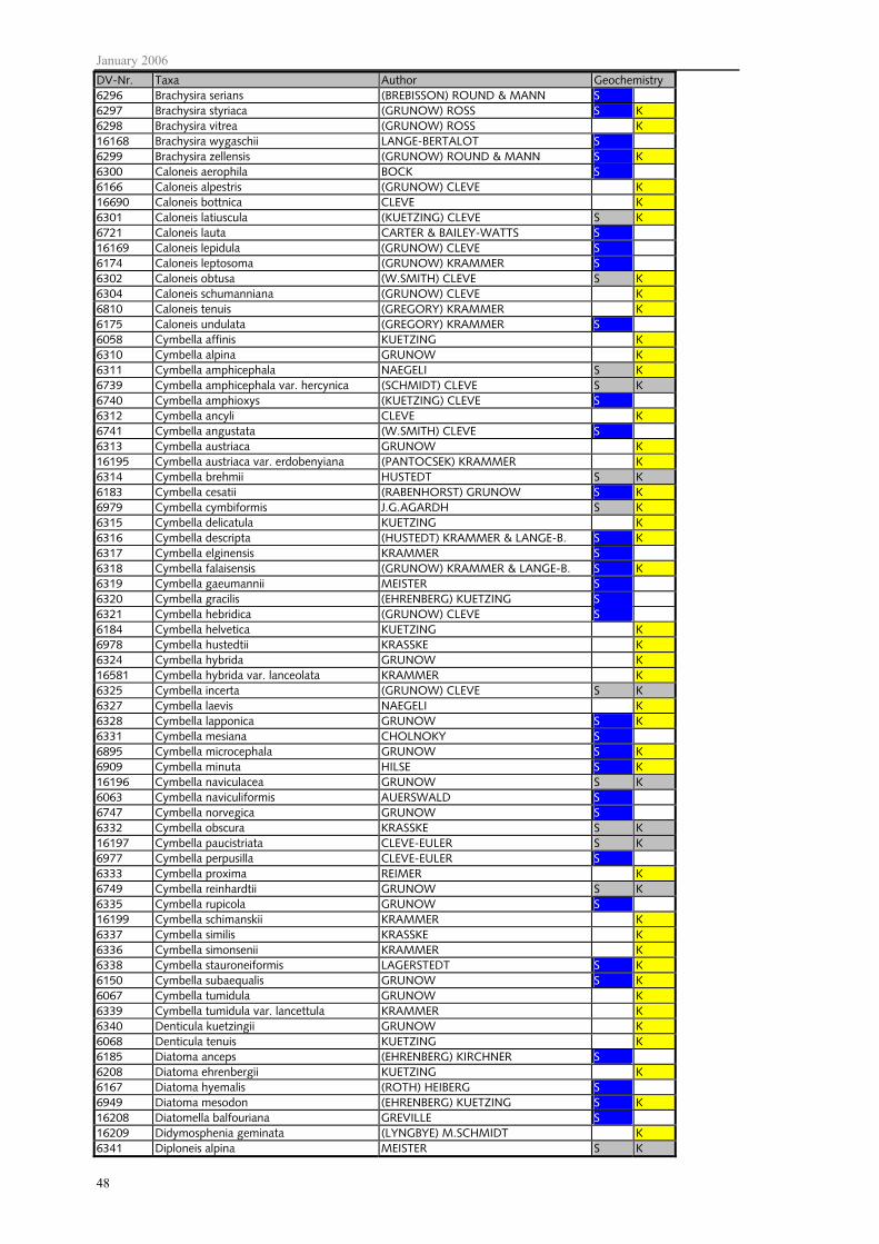
January 2006

48

DV-Nr. Taxa Author Geochemistry 6296 Brachysira serians (BREBISSON) ROUND & MANN S 6297 Brachysira styriaca (GRUNOW) ROSS S K 6298 Brachysira vitrea (GRUNOW) ROSS K 16168 Brachysira wygaschii LANGE-BERTALOT S 6299 Brachysira zellensis (GRUNOW) ROUND & MANN S K 6300 Caloneis aerophila BOCK S 6166 Caloneis alpestris (GRUNOW) CLEVE K 16690 Caloneis bottnica CLEVE K 6301 Caloneis latiuscula (KUETZING) CLEVE S K 6721 Caloneis lauta CARTER & BAILEY-WATTS S 16169 Caloneis lepidula (GRUNOW) CLEVE S 6174 Caloneis leptosoma (GRUNOW) KRAMMER S 6302 Caloneis obtusa (W.SMITH) CLEVE S K 6304 Caloneis schumanniana (GRUNOW) CLEVE K 6810 Caloneis tenuis (GREGORY) KRAMMER K 6175 Caloneis undulata (GREGORY) KRAMMER S 6058 Cymbella affinis KUETZING K 6310 Cymbella alpina GRUNOW K 6311 Cymbella amphicephala NAEGELI S K 6739 Cymbella amphicephala var. hercynica (SCHMIDT) CLEVE S K 6740 Cymbella amphioxys (KUETZING) CLEVE S 6312 Cymbella ancyli CLEVE K 6741 Cymbella angustata (W.SMITH) CLEVE S 6313 Cymbella austriaca GRUNOW K 16195 Cymbella austriaca var. erdobenyiana (PANTOCSEK) KRAMMER K 6314 Cymbella brehmii HUSTEDT S K 6183 Cymbella cesatii (RABENHORST) GRUNOW S K 6979 Cymbella cymbiformis J.G.AGARDH S K 6315 Cymbella delicatula KUETZING K 6316 Cymbella descripta (HUSTEDT) KRAMMER & LANGE-B. S K 6317 Cymbella elginensis KRAMMER S 6318 Cymbella falaisensis (GRUNOW) KRAMMER & LANGE-B. S K 6319 Cymbella gaeumannii MEISTER S 6320 Cymbella gracilis (EHRENBERG) KUETZING S 6321 Cymbella hebridica (GRUNOW) CLEVE S 6184 Cymbella helvetica KUETZING K 6978 Cymbella hustedtii KRASSKE K 6324 Cymbella hybrida GRUNOW K 16581 Cymbella hybrida var. lanceolata KRAMMER K 6325 Cymbella incerta (GRUNOW) CLEVE S K 6327 Cymbella laevis NAEGELI K 6328 Cymbella lapponica GRUNOW S K 6331 Cymbella mesiana CHOLNOKY S 6895 Cymbella microcephala GRUNOW S K 6909 Cymbella minuta HILSE S K 16196 Cymbella naviculacea GRUNOW S K 6063 Cymbella naviculiformis AUERSWALD S 6747 Cymbella norvegica GRUNOW S 6332 Cymbella obscura KRASSKE S K 16197 Cymbella paucistriata CLEVE-EULER S K 6977 Cymbella perpusilla CLEVE-EULER S 6333 Cymbella proxima REIMER K 6749 Cymbella reinhardtii GRUNOW S K 6335 Cymbella rupicola GRUNOW S 16199 Cymbella schimanskii KRAMMER K 6337 Cymbella similis KRASSKE K 6336 Cymbella simonsenii KRAMMER K 6338 Cymbella stauroneiformis LAGERSTEDT S K 6150 Cymbella subaequalis GRUNOW S K 6067 Cymbella tumidula GRUNOW K 6339 Cymbella tumidula var. lancettula KRAMMER K 6340 Denticula kuetzingii GRUNOW K 6068 Denticula tenuis KUETZING K 6185 Diatoma anceps (EHRENBERG) KIRCHNER S 6208 Diatoma ehrenbergii KUETZING K 6167 Diatoma hyemalis (ROTH) HEIBERG S 6949 Diatoma mesodon (EHRENBERG) KUETZING S K 16208 Diatomella balfouriana GREVILLE S 16209 Didymosphenia geminata (LYNGBYE) M.SCHMIDT K 6341 Diploneis alpina MEISTER S K

Janurary 2006

49

DV-Nr. Taxa Author Geochemistry 6807 Diploneis elliptica (KUETZING) CLEVE K 6345 Diploneis modica HUSTEDT K 6346 Diploneis oblongella (NAEGELI) CLEVE-EULER K 6070 Diploneis ovalis (HILSE) CLEVE K 6348 Diploneis parma CLEVE S 6349 Diploneis petersenii HUSTEDT S 6754 Entomoneis ornata (BAILEY) REIMER S K 6351 Epithemia goeppertiana HILSE K 6352 Epithemia smithii CARRUTHERS K 16666 Eunotia angusta (GRUNOW) BERG S 6354 Eunotia arcubus NOERPEL & LANGE-BERTALOT K 16221 Eunotia arculus (GRUNOW) LANGE-B. & NOERPEL S 6886 Eunotia arcus EHRENBERG S 6213 Eunotia bilunaris (EHRENBERG) MILLS S K 16222 Eunotia bilunaris var. linearis (OKUNO) LANGE-B. & NOERPEL S 6355 Eunotia bilunaris var. mucophila LANGE-BERTALOT & NOERPEL S 6761 Eunotia botuliformis WILD et al. S 16223 Eunotia circumborealis LANGE-BERTALOT & NOERPEL S 6356 Eunotia denticulata (BREBISSON) RABENHORST S 6357 Eunotia diodon EHRENBERG S 16224 Eunotia elegans OESTRUP S 6975 Eunotia exigua (BREBISSON) RABENHORST S 16225 Eunotia exigua var. undulata MAGDEBURG S 6358 Eunotia faba EHRENBERG S 6359 Eunotia fallax A.CLEVE S 6360 Eunotia flexuosa (BREBISSON) KUETZING S 6362 Eunotia glacialis MEISTER S 6363 Eunotia hexaglyphis EHRENBERG S 6364 Eunotia implicata NOERPEL et al. S 6214 Eunotia incisa GREGORY S 6365 Eunotia intermedia (KRASSKE) NOERPEL & LANGE-B. S 16226 Eunotia islandica OESTRUP S 16104 Eunotia jemtlandica (FONTELL) BERG S 16228 Eunotia major (W.SMITH) RABENHORST S 6367 Eunotia meisteri HUSTEDT S 6368 Eunotia microcephala KRASSKE S 6369 Eunotia minor (KUETZING) GRUNOW S K 6885 Eunotia monodon EHRENBERG S 6370 Eunotia muscicola var. tridentula NOERPEL & LANGE-BERTALOT S 6371 Eunotia naegelii MIGULA S 16695 Eunotia neofallax NOERPEL S 6372 Eunotia nymanniana GRUNOW S 6373 Eunotia paludosa GRUNOW S 6884 Eunotia paludosa var. trinacria (KRASSKE) NOERPEL S 6168 Eunotia pectinalis (DILLWYN) RABENHORST S 6766 Eunotia pectinalis var. undulata (RALFS) RABENHORST S 6851 Eunotia praerupta EHRENBERG S 6374 Eunotia praerupta var. bigibba (KUETZING) GRUNOW S 6768 Eunotia praerupta var. curta GRUNOW S 6769 Eunotia praerupta var. inflata GRUNOW S 16229 Eunotia pseudopectinalis HUSTEDT S 6375 Eunotia rhomboidea HUSTEDT S 16230 Eunotia rhynchocephala HUSTEDT S 6376 Eunotia septentrionalis OESTRUP S 6850 Eunotia serra EHRENBERG S 6770 Eunotia serra var. diadema (EHRENBERG) PATRICK S 6377 Eunotia serra var. tetraodon (EHRENBERG) NOERPEL S 6378 Eunotia silvahercynia NOERPEL et al. S 6379 Eunotia soleirolii (KUETZING) RABENHORST S 6380 Eunotia steineckei PETERSEN S 6381 Eunotia subarcuatoides ALLES et al. S 6382 Eunotia sudetica O.MUELLER S 6383 Eunotia tenella (GRUNOW) HUSTEDT S 6771 Eunotia triodon EHRENBERG S 16233 Fragilaria acidoclinata LANGE-BERTALOT & HOFMANN S 6077 Fragilaria arcus (EHRENBERG) CLEVE S K 6908 Fragilaria capucina var. amphicephala (GRUNOW) LANGE-BERTALOT K 6389 Fragilaria capucina var. austriaca (GRUNOW) LANGE-BERTALOT K 6392 Fragilaria capucina var. gracilis (OESTRUP) HUSTEDT S K 6396 Fragilaria capucina var. rumpens (KUETZING) LANGE-BERTALOT S K

January 2006

50

DV-Nr. Taxa Author Geochemistry 16234 Fragilaria constricta EHRENBERG S 6399 Fragilaria delicatissima (W.SMITH) LANGE-BERTALOT K 6401 Fragilaria exigua GRUNOW S 6405 Fragilaria nanana LANGE-BERTALOT S K 6407 Fragilaria pseudoconstruens MARCINIAK S 6409 Fragilaria tenera (W.SMITH) LANGE-BERTALOT S K 6169 Fragilaria virescens RALFS S 6187 Frustulia rhomboides (EHRENBERG) DE TONI S 6412 Frustulia rhomboides var. crassinervia (BREBISSON) ROSS S 6413 Frustulia rhomboides var. saxonica (RABENHORST) DE TONI S 6414 Frustulia rhomboides var. viridula (BREBISSON) CLEVE S 6417 Gomphonema acutiusculum (O.MUELLER) CLEVE-EULER S K 16246 Gomphonema amoenum LANGE-BERTALOT S 6819 Gomphonema angustum J.G.AGARDH K 6419 Gomphonema auritum A.BRAUN S K 6420 Gomphonema bavaricum REICHARDT & LANGE-BERTALOT K 6421 Gomphonema bohemicum REICHELT & FRICKE S 6423 Gomphonema dichotomum KUETZING S K 6424 Gomphonema hebridense GREGORY S 6425 Gomphonema helveticum BRUN K 16661 Gomphonema lacus-vulcani REICHARDT & LANGE-BERTALOT S 6426 Gomphonema lagerheimii A.CLEVE S 6427 Gomphonema lateripunctatum REICHARDT & LANGE-BERTALOT K 6429 Gomphonema occultum REICHARDT & LANGE-BERTALOT K 6430 Gomphonema olivaceum v. minutissimum HUSTEDT S 6431 Gomphonema olivaceum v. olivaceoides (HUSTEDT) LANGE-B. & REICHARDT S K 6433 Gomphonema parvulum var. exilissimum GRUNOW S K 16258 Gomphonema parvulum var. parvulius LANGE-BERTALOT & REICHARDT S K 6434 Gomphonema procerum REICHARDT & LANGE-BERTALOT K 6435 Gomphonema productum (GRUNOW) LANGE-B. & REICHARDT S 16586 Gomphonema rhombicum FRICKE S 6440 Gomphonema subtile EHRENBERG S K 6441 Gomphonema tenue FRICKE K 6999 Gomphonema ventricosum GREGORY S K 6442 Gomphonema vibrio EHRENBERG K 6804 Mastogloia grevillei W.SMITH K 6445 Mastogloia smithii var. lacustris GRUNOW K 6446 Meridion circulare var. constrictum (RALFS) VAN HEURCK S K 6448 Navicula absoluta HUSTEDT S K 16717 Navicula adversa KRASSKE S 6809 Navicula angusta GRUNOW S 16289 Navicula aquaedurae LANGE-BERTALOT K 6460 Navicula brockmannii HUSTEDT S 6461 Navicula bryophila PETERSEN S K 6464 Navicula catalanogermanica LANGE-BERTALOT & HOFMANN S K 16300 Navicula cataractarheni LANGE-BERTALOT K 6969 Navicula cocconeiformis GREGORY S K 6468 Navicula concentrica CARTER S K 6472 Navicula dealpina LANGE-BERTALOT K 16308 Navicula declivis HUSTEDT S 6474 Navicula densilineolata (LANGE-B.) LANGE-BERTALOT K 6475 Navicula detenta HUSTEDT S 16000 Navicula digitulus HUSTEDT S 6478 Navicula diluviana KRASSKE K 16001 Navicula disjuncta HUSTEDT S 6482 Navicula evanida HUSTEDT S 6917 Navicula exilis KUETZING S 6485 Navicula festiva KRASSKE S 6489 Navicula gallica var. perpusilla (GRUNOW) LANGE-BERTALOT S 6493 Navicula gotlandica GRUNOW K 6496 Navicula heimansioides LANGE-BERTALOT S 16324 Navicula hoefleri CHOLNOKY S 6501 Navicula ignota var. acceptata (HUSTEDT) LANGE-BERTALOT S K 6502 Navicula ignota var. palustris (HUSTEDT) LUND S 6505 Navicula jaagii MEISTER S K 6506 Navicula jaernefeltii HUSTEDT K 6509 Navicula krasskei HUSTEDT S 6882 Navicula laevissima KUETZING S K 16010 Navicula lapidosa KRASSKE S 16334 Navicula laticeps HUSTEDT K

Janurary 2006

51

DV-Nr. Taxa Author Geochemistry 16335 Navicula leistikowii LANGE-BERTALOT K 6923 Navicula lenzii HUSTEDT K 16011 Navicula leptostriata JOERGENSEN S 16337 Navicula levanderii HUSTEDT S 6511 Navicula lundii REICHARDT S K 16012 Navicula maceria SCHIMANSKI S 16342 Navicula mediocostata REICHARDT K 6513 Navicula mediocris KRASSKE S 6515 Navicula minuscula GRUNOW S 16349 Navicula notha WALLACE S 6521 Navicula oligotraphenta LANGE-BERTALOT & HOFMANN K 16356 Navicula porifera var. opportuna (HUSTEDT) LANGE-BERTALOT S 6524 Navicula praeterita HUSTEDT K 6527 Navicula pseudobryophila (HUSTEDT) HUSTEDT S 6529 Navicula pseudoscutiformis HUSTEDT S K 16028 Navicula pseudosilicula HUSTEDT S 6530 Navicula pseudotuscula HUSTEDT K 6533 Navicula pusio CLEVE S 6536 Navicula rotunda HUSTEDT S 6538 Navicula schadei KRASSKE K 6539 Navicula schmassmannii HUSTEDT S 6926 Navicula schoenfeldii HUSTEDT K 6543 Navicula soehrensis KRASSKE S 16034 Navicula soehrensis var. hassiaca (KRASSKE) LANGE-BERTALOT S 6544 Navicula soehrensis var. muscicola (PETERSEN) KRASSKE S 16035 Navicula stankovicii HUSTEDT K 6546 Navicula stroemii HUSTEDT K 6547 Navicula subalpina REICHARDT K 6549 Navicula submolesta HUSTEDT S 6878 Navicula subtilissima CLEVE S 6551 Navicula suchlandtii HUSTEDT S 6554 Navicula tridentula KRASSKE S 6989 Navicula tuscula (EHRENBERG) GRUNOW K 6556 Navicula utermoehlii HUSTEDT K 16037 Navicula variostriata KRASSKE S 16736 Navicula ventraloconfusa LANGE-BERTALOT S 6560 Navicula vulpina KUETZING K 6561 Navicula wildii LANGE-BERTALOT K 6820 Neidium affine (EHRENBERG) PFITZER S K 6562 Neidium affine var. longiceps (GREGORY) CLEVE S K 6563 Neidium alpinum HUSTEDT S 6564 Neidium ampliatum (EHRENBERG) KRAMMER S K 6566 Neidium bisulcatum (LAGERSTEDT) CLEVE S 6567 Neidium carterii KRAMMER S 16383 Neidium densestriatum (OESTRUP) KRAMMER S 6568 Neidium hercynicum A.MAYER S 6109 Neidium iridis (EHRENBERG) CLEVE S 16386 Neidium ladogensis (CLEVE) FOGED S 6110 Neidium productum (W.SMITH) CLEVE S 6571 Neidium septentrionale CLEVE-EULER S 6573 Nitzschia acidoclinata LANGE-BERTALOT S K 6575 Nitzschia alpina HUSTEDT S 16100 Nitzschia alpinobacillum LANGE-BERTALOT S K 6577 Nitzschia bacilliformis HUSTEDT K 16396 Nitzschia bryophila (HUSTEDT) HUSTEDT S 16579 Nitzschia dissipata ssp. oligotraphenta LANGE-BERTALOT S K 6586 Nitzschia dissipata var. media (HANTZSCH) GRUNOW S K 6587 Nitzschia diversa HUSTEDT K 6589 Nitzschia fibulafissa LANGE-BERTALOT K 16749 Nitzschia garrensis HUSTEDT S 6592 Nitzschia gessneri HUSTEDT K 6593 Nitzschia gisela LANGE-BERTALOT K 6931 Nitzschia hantzschiana RABENHORST S K 16051 Nitzschia homburgiensis LANGE-BERTALOT S 6597 Nitzschia lacuum LANGE-BERTALOT S K 16433 Nitzschia paleaeformis HUSTEDT S 6605 Nitzschia perminuta (GRUNOW) M.PERAGALLO S K 6607 Nitzschia radicula HUSTEDT K 6608 Nitzschia regula HUSTEDT K 16455 Nupela rhetica (WUETHRICH) LANGE-BERTALOT S K

January 2006

52

DV-Nr. Taxa Author Geochemistry 16456 Nupela tenuicephala (HUSTEDT) LANGE-BERTALOT S 6619 Peronia fibula (BREBISSON) ROSS S 6620 Pinnularia acoricola HUSTEDT S 6877 Pinnularia acuminata W.SMITH S 6621 Pinnularia anglica KRAMMER S 6622 Pinnularia angusta (CLEVE) KRAMMER S 16543 Pinnularia bacilliformis KRAMMER S 16461 Pinnularia balfouriana GRUNOW S K 6624 Pinnularia brandeliformis KRAMMER S 6625 Pinnularia brandelii CLEVE S 16463 Pinnularia brauniana (GRUNOW) MILLS S 6881 Pinnularia braunii (GRUNOW) CLEVE S 6627 Pinnularia brevicostata CLEVE S 16062 Pinnularia cardinalis (EHRENBERG) W.SMITH S 16544 Pinnularia carminata BARBER & CARTER S 6629 Pinnularia cleveiformis KRAMMER S 6632 Pinnularia divergens W.SMITH S 16466 Pinnularia divergens var. decrescens (GRUNOW) KRAMMER S 6633 Pinnularia divergentissima (GRUNOW) CLEVE S 6845 Pinnularia episcopalis CLEVE S 16063 Pinnularia esox EHRENBERG S 16546 Pinnularia esoxiformis FUSEY S 16547 Pinnularia esoxiformis var. eifeliana KRAMMER S 6636 Pinnularia gentilis (DONKIN) CLEVE S 6121 Pinnularia gibba EHRENBERG S K 6638 Pinnularia gibbiformis KRAMMER S K 16065 Pinnularia gigas EHRENBERG S 6223 Pinnularia hemiptera (KUETZING) RABENHORST S K 6642 Pinnularia infirma KRAMMER S K 6643 Pinnularia intermedia (LAGERSTEDT) CLEVE S 6844 Pinnularia interrupta W.SMITH S 6853 Pinnularia lata (BREBISSON) RABENHORST S 6958 Pinnularia legumen EHRENBERG S K 6648 Pinnularia macilenta (EHRENBERG) EHRENBERG S K 6123 Pinnularia maior (KUETZING) RABENHORST S 6124 Pinnularia mesolepta (EHRENBERG) W.SMITH S K 16475 Pinnularia mesolepta var. gibberula (HUSTEDT) KRAMMER S K 6125 Pinnularia microstauron (EHRENBERG) CLEVE S 6651 Pinnularia neomajor KRAMMER S 6111 Pinnularia nobilis (EHRENBERG) EHRENBERG S 6652 Pinnularia nodosa (EHRENBERG) W.SMITH S 6653 Pinnularia notabilis KRAMMER S 6654 Pinnularia obscura KRASSKE S K 6655 Pinnularia oriunda KRAMMER S K 6656 Pinnularia parallela BRUN S K 16070 Pinnularia platycephala (EHRENBERG) CLEVE S 6842 Pinnularia polyonca (BREBISSON) W.SMITH S 6658 Pinnularia pseudogibba KRAMMER S 16552 Pinnularia renata KRAMMER S 6659 Pinnularia rupestris HANTZSCH S 6660 Pinnularia schoenfelderi KRAMMER S 16074 Pinnularia silvatica PETERSEN S 16075 Pinnularia similiformis KRAMMER S 6662 Pinnularia sinistra KRAMMER S 6663 Pinnularia stomatophora (GRUNOW) CLEVE S 16479 Pinnularia stomatophora var. triundulata (FONTELL) HUSTEDT S 6664 Pinnularia streptoraphe CLEVE S 16480 Pinnularia streptoraphe var. parva KRAMMER S 6126 Pinnularia subcapitata GREGORY S 16481 Pinnularia subcapitata var. elongata KRAMMER S 6665 Pinnularia subcapitata var. hilseana (JANISCH) O.MUELLER S 6667 Pinnularia subgibba KRAMMER S K 16482 Pinnularia subgibba var. hustedtii KRAMMER S K 16483 Pinnularia subgibba var. undulata KRAMMER S K 6670 Pinnularia subrupestris KRAMMER S 16557 Pinnularia subrupestris var. parva KRAMMER S 6671 Pinnularia suchlandtii HUSTEDT S 6673 Pinnularia transversa (A.SCHMIDT) MAYER S 6674 Pinnularia viridiformis KRAMMER S 6128 Pinnularia viridis (NITZSCH) EHRENBERG S K

Janurary 2006

53

DV-Nr. Taxa Author Geochemistry 6676 Pinnularia woerthensis (MAYER) KRAMMER S 6678 Rhopalodia gibba var. parallela (GRUNOW) H.ET M.PERAGALLO K 16495 Rhopalodia rupestris (W.SMITH) KRAMMER S 6129 Stauroneis anceps EHRENBERG S 6680 Stauroneis anceps var. gracilis (EHRENBERG) BRUN S 6681 Stauroneis kriegerii PATRICK S K 6840 Stauroneis nobilis SCHUMANN S 6688 Stauroneis thermicola (PETERSEN) LUND S K 6689 Stauroneis undata HUSTEDT S 16087 Stenopterobia curvula (W.SMITH) KRAMMER S 6690 Stenopterobia delicatissima (LEWIS) BREBISSON S 16503 Stenopterobia densestriata (HUSTEDT) KRAMMER S 16507 Surirella barrowcliffia DONKIN S 6691 Surirella bifrons EHRENBERG S K 6135 Surirella linearis W.SMITH S K 16091 Surirella linearis var. helvetica (BRUN) MEISTER S K 6694 Surirella roba LECLERCQ S 6137 Surirella robusta EHRENBERG S 6097 Surirella spiralis KUETZING S K 16092 Surirella tenera GREGORY S K 16518 Surirella turgida W.SMITH S K 16519 Tabellaria binalis (EHRENBERG) GRUNOW S 6091 Tabellaria flocculosa (ROTH) KUETZING S K 16096 Tabellaria quadriseptata KNUDSON S 6698 Tabellaria ventricosa KUETZING S 16521 Tetracyclus emarginatus (EHRENBERG) W.SMITH S 16522 Tetracyclus glans (EHRENBERG) MILLS S 16097 Tetracyclus rupestris (BRAUN) GRUNOW S

Table 25: Species specific parameters for calculation of the Trophic Index and the Saprobic Index according to ROTT et al. (1997, 1999). TW = Trophic value; SW = Saprobic value; G = Weighting. If no varieties are mentioned the type varieties are meant.

DV-Nr. Taxa Author TW G SW G

6699 Achnanthes altaica (PORETZKY) CLEVE-EULER 1,7 2 1,0 5 6139 Achnanthes biasolettiana GRUNOW 1,3 1 1,4 3 6835 Achnanthes bioretii GERMAIN 1,2 4 6180 Achnanthes clevei GRUNOW 1,6 3 6247 Achnanthes coarctata (BREBISSON) GRUNOW 0,9 2 6855 Achnanthes conspicua A.MAYER 1,5 2 16110 Achnanthes curtissima CARTER 0,6 2 16111 Achnanthes daonensis LANGE-BERTALOT 1,1 4 6248 Achnanthes delicatula (KUETZING) GRUNOW 2,9 3 2,6 3 16112 Achnanthes delicatula ssp. engelbrechtii (CHOLNOKY) LANGE-BERTALOT 2,0 3 6249 Achnanthes exilis KUETZING 1,2 3 1,3 4 6250 Achnanthes flexella (KUETZING) BRUN 0,3 3 1,0 5 6251 Achnanthes flexella var. alpestris BRUN 1,0 5 6253 Achnanthes helvetica (HUSTEDT) LANGE-BERTALOT 0,6 3 1,0 5 6047 Achnanthes hungarica (GRUNOW) GRUNOW 3,4 2 2,7 3 6703 Achnanthes kolbei HUSTEDT 3,9 2 6258 Achnanthes laevis OESTRUP 1,2 2 1,3 3 6260 Achnanthes lanceolata ssp. frequentissima LANGE-BERTALOT 2,8 3 16127 Achnanthes lanceolata ssp. lanceolata (BREBISSON) GRUNOW 3,3 3 6262 Achnanthes lapidosa KRASSKE 0,7 3 1,0 5 6705 Achnanthes laterostrata HUSTEDT 1,2 2 1,0 5 6263 Achnanthes lauenburgiana HUSTEDT 1,8 3 1,9 4 6264 Achnanthes levanderi HUSTEDT 0,6 3 1,0 5 6045 Achnanthes linearis (W.SMITH) GRUNOW 1,8 1 6265 Achnanthes marginulata GRUNOW 0,6 2 1,0 5 6266 Achnanthes minuscula HUSTEDT 2,3 2 1,9 4 6014 Achnanthes minutissima KUETZING 1,2 1 1,7 1 6173 Achnanthes minutissima var. affinis (GRUNOW) LANGE-BERTALOT 2,3 2 1,3 3 6240 Achnanthes minutissima var. gracillima (MEISTER) LANGE-BERTALOT 0,6 3 1,0 5 6707 Achnanthes minutissima var. jackii (RABENHORST) LANGE-BERTALOT 1,2 3 16135 Achnanthes minutissima var. saprophila KOBAYASI et MAYAMA 2,7 4 3,1 3 6267 Achnanthes minutissima var. scotica (CARTER) LANGE-BERTALOT 1,0 2 1,0 5 6708 Achnanthes montana KRASSKE 0,6 2 1,0 5 6709 Achnanthes nodosa CLEVE 0,6 2 1,0 5

January 2006

54


6268 Achnanthes oblongella OESTRUP 1,0 2 1,0 5 6269 Achnanthes oestrupii (CLEVE-EULER) HUSTEDT 1,2 2 1,3 4 6270 Achnanthes peragalli BRUN et HERIBAUD 0,6 3 1,1 4 6271 Achnanthes petersenii HUSTEDT 0,6 1 1,0 5 6984 Achnanthes ploenensis HUSTEDT 2,6 3 1,9 4 6272 Achnanthes pusilla (GRUNOW) DE TONI 0,6 3 1,0 5 6711 Achnanthes rechtensis LECLERCQ 0,6 2 1,0 5 6712 Achnanthes rupestoides HOHN 1,2 3 16144 Achnanthes rupestris KRASSKE 0,6 2 6276 Achnanthes subatomoides (HUST.) LANGE-B. et ARCHIBALD 2,1 2 1,1 4 16148 Achnanthes subsalsa PETERSEN 0,6 2 6277 Achnanthes suchlandtii HUSTEDT 0,6 2 1,0 5 6279 Achnanthes trinodis (W.SMITH) GRUNOW 0,6 2 1,0 5 6048 Amphipleura pellucida (KUETZING) KUETZING 2,1 2 1,3 3 6281 Amphipleura rutilans (TRENTEPOHL) CLEVE 2,9 3 6171 Amphora inariensis KRAMMER 2,1 1 1,2 4 6860 Amphora libyca EHRENBERG 3,5 5 1,6 2 6286 Amphora montana KRASSKE 2,9 2 6044 Amphora ovalis (KUETZING) KUETZING 3,3 2 1,5 2 6983 Amphora pediculus (KUETZING) GRUNOW 2,8 2 2,1 2 6288 Amphora thumensis (A.MAYER) CLEVE-EULER 1,4 3 1,1 4 6181 Amphora veneta KUETZING 3,8 2 3,6 3 6049 Anomoeoneis sphaerophora (EHRENBERG) PFITZER 3,4 3 2,7 3 6050 Asterionella formosa HASSALL 1,8 2 1,5 3 6799 Aulacoseira distans (EHRENBERG) SIMONSEN 1,0 4 6787 Aulacoseira italica (EHRENBERG) SIMONSEN 1,4 2 6716 Aulacoseira lirata (EHRENBERG) ROSS 1,8 2 6143 Bacillaria paradoxa GMELIN 2,9 3 2,3 3 6291 Brachysira brebissonii ROSS 1,1 2 1,0 5 6295 Brachysira neoexilis LANGE-BERTALOT 1,2 2 1,1 5 6296 Brachysira serians (BREBISSON) ROUND et MANN 0,6 1 1,0 5 6298 Brachysira vitrea (GRUNOW) ROSS 0,7 2 1,0 5 6300 Caloneis aerophila BOCK 1,0 5 6166 Caloneis alpestris (GRUNOW) CLEVE 1,3 2 1,0 5 6043 Caloneis amphisbaena (BORY DE SAINT VINCENT) CLEVE 3,9 2 2,3 3 6051 Caloneis bacillum (GRUNOW) CLEVE 2,5 1 2,0 4 6301 Caloneis latiuscula (KUETZING) CLEVE 1,0 5 6302 Caloneis obtusa (W.SMITH) CLEVE 0,6 2 1,0 5 6303 Caloneis pulchra MESSIKOMMER 1,2 1 1,0 5 6304 Caloneis schumanniana (GRUNOW) CLEVE 1,2 4 6052 Caloneis silicula (EHRENBERG) CLEVE 1,2 4 6723 Caloneis sublinearis (GRUNOW) KRAMMER 1,0 5 6810 Caloneis tenuis (GREGORY) KRAMMER 1,1 2 6175 Caloneis undulata (GREGORY) KRAMMER 0,6 2 6053 Campylodiscus noricus EHRENBERG 2,3 1 6981 Cocconeis disculus (SCHUMANN) CLEVE 2,2 3 6306 Cocconeis neothumensis KRAMMER 2,0 2 1,5 3 6020 Cocconeis pediculus EHRENBERG 2,6 2 2,0 3 6021 Cocconeis placentula EHRENBERG 2,6 2 1,8 2 6726 Cocconeis placentula var. euglypta EHRENBERG 2,3 2 6727 Cocconeis placentula var. klinoraphis GEITLER 2,3 2 6728 Cocconeis placentula var. lineata (EHRENBERG) VAN HEURCK 2,3 2 6307 Cocconeis pseudothumensis REICHARDT 1,0 5 6943 Cyclostephanos dubius (FRICKE) ROUND 2,9 3 6002 Cyclotella meneghiniana KUETZING 2,8 5 6936 Cyclotella ocellata PANTOCSEK 1,5 1 6057 Cymatopleura elliptica (BREBISSON) W.SMITH 2,9 3 1,4 3 6031 Cymatopleura solea (BREBISSON) W.SMITH 3,1 3 2,1 3 6738 Cymbella aequalis W.SMITH 0,6 2 6058 Cymbella affinis KUETZING 0,7 4 1,2 4 6310 Cymbella alpina GRUNOW 0,6 3 1,0 5 6311 Cymbella amphicephala NAEGELI 1,1 3 1,1 4 6739 Cymbella amphicephala var. hercynica (SCHMIDT) CLEVE 0,9 2 6740 Cymbella amphioxys (KUETZING) CLEVE 0,6 2 6312 Cymbella ancyli CLEVE 0,9 2 6741 Cymbella angustata (W.SMITH) CLEVE 0,9 2 1,0 5 6092 Cymbella aspera (EHRENBERG) CLEVE 1,7 1 6313 Cymbella austriaca GRUNOW 0,6 1 1,0 5 6891 Cymbella caespitosa (KUETZING) BRUN 1,6 2

Janurary 2006

55


6183 Cymbella cesatii (RABENHORST) GRUNOW 0,6 4 1,0 5 6059 Cymbella cistula (EHRENBERG) KIRCHNER 2,3 1 1,4 3 6060 Cymbella cuspidata KUETZING 1,1 4 6979 Cymbella cymbiformis J.G.AGARDH 1,8 3 1,0 5 6315 Cymbella delicatula KUETZING 0,3 4 1,0 5 6316 Cymbella descripta (HUSTEDT) KRAMMER et LANGE-B. 0,6 2 1,0 5 6061 Cymbella ehrenbergii KUETZING 2,2 3 1,1 4 6317 Cymbella elginensis KRAMMER 0,6 2 6318 Cymbella falaisensis (GRUNOW) KRAMMER et LANGE-B. 0,4 3 1,0 5 6319 Cymbella gaeumannii MEISTER 0,6 2 1,0 5 6320 Cymbella gracilis (EHRENBERG) KUETZING 0,6 4 1,0 5 6321 Cymbella hebridica (GRUNOW) CLEVE 0,6 2 1,0 5 6184 Cymbella helvetica KUETZING 1,4 2 1,1 4 6323 Cymbella helvetica var. compacta (OESTRUP) HUSTEDT 2,6 3 1,8 3 6978 Cymbella hustedtii KRASSKE 1,2 2 6324 Cymbella hybrida GRUNOW 0,6 2 1,0 5 6325 Cymbella incerta (GRUNOW) CLEVE 0,6 2 1,0 5 6327 Cymbella laevis NAEGELI 0,9 2 1,0 5 6062 Cymbella lanceolata (EHRENBERG) KIRCHNER 1,6 4 6330 Cymbella leptoceros (EHRENBERG) KUETZING 1,3 4 6331 Cymbella mesiana CHOLNOKY 1,0 5 6895 Cymbella microcephala GRUNOW 1,2 1 1,2 4 6909 Cymbella minuta HILSE 2,0 1 1,6 2 6063 Cymbella naviculiformis AUERSWALD 1,8 1 1,3 3 6747 Cymbella norvegica GRUNOW 0,6 2 1,0 5 6977 Cymbella perpusilla CLEVE-EULER 0,5 2 1,0 5 6040 Cymbella prostrata (BERKELEY) CLEVE 2,3 1 1,8 3 6333 Cymbella proxima REIMER 1,2 2 1,1 5 6748 Cymbella pusilla GRUNOW 1,2 2 6334 Cymbella reichardtii KRAMMER 2,7 3 1,5 4 6335 Cymbella rupicola GRUNOW 1,0 5 6337 Cymbella similis KRASSKE 0,6 2 1,0 5 6336 Cymbella simonsenii KRAMMER 0,6 2 1,0 5 6065 Cymbella sinuata GREGORY 2,1 1 2,0 2 6150 Cymbella subaequalis GRUNOW 1,0 2 1,0 5 6066 Cymbella tumida (BREBISSON) VAN HEURCK 2,5 2 1,6 4 6067 Cymbella tumidula GRUNOW 0,6 2 1,0 5 6339 Cymbella tumidula var. lancettula KRAMMER 0,3 2 1,0 5 6752 Denticula elegans KUETZING 1,8 2 6340 Denticula kuetzingii GRUNOW 1,0 2 1,0 5 6068 Denticula tenuis KUETZING 1,4 3 1,3 4 6185 Diatoma anceps (EHRENBERG) KIRCHNER 0,3 2 1,0 5 6208 Diatoma ehrenbergii KUETZING 1,6 2 1,3 3 6167 Diatoma hyemalis (ROTH) HEIBERG 1,0 4 1,0 5 6949 Diatoma mesodon (EHRENBERG) KUETZING 0,7 4 1,3 4 6209 Diatoma moniliformis KUETZING 2,0 3 2,2 4 6210 Diatoma tenuis J.G.AGARDH 1,3 4 6006 Diatoma vulgaris BORY DE SAINT VINCENT 2,1 4 16208 Diatomella balfouriana GREVILLE 0,6 2 1,0 5 16209 Didymosphenia geminata (LYNGBYE) M.SCHMIDT 0,6 1 6807 Diploneis elliptica (KUETZING) CLEVE 1,7 2 1,1 4 6346 Diploneis oblongella (NAEGELI) CLEVE-EULER 1,0 2 1,0 5 6347 Diploneis oculata (BREBISSON) CLEVE 1,2 4 6070 Diploneis ovalis (HILSE) CLEVE 1,0 2 1,0 5 6349 Diploneis petersenii HUSTEDT 1,3 2 1,1 4 6754 Entomoneis ornata (BAILEY) REIMER 1,2 2 6212 Epithemia adnata (KUETZING) BREBISSON 2,2 2 1,2 4 6350 Epithemia argus (EHRENBERG) KUETZING 1,1 2 6887 Epithemia sorex KUETZING 2,7 2 1,4 3 6353 Epithemia turgida (EHRENBERG) KUETZING 2,3 2 6354 Eunotia arcubus NOERPEL et LANGE-BERTALOT 0,6 2 1,0 5 16221 Eunotia arculus (GRUNOW) LANGE-B. et NOERPEL 1,1 2 6886 Eunotia arcus EHRENBERG 1,0 5 6213 Eunotia bilunaris (EHRENBERG) MILLS 1,7 2 6357 Eunotia diodon EHRENBERG 0,6 2 1,0 5 6975 Eunotia exigua (BREBISSON) RABENHORST 0,5 3 1,1 4 6359 Eunotia fallax A.CLEVE 0,6 2 1,0 5 6360 Eunotia flexuosa (BREBISSON) KUETZING 0,7 2 1,0 5 6362 Eunotia glacialis MEISTER 0,7 2 1,0 5

January 2006

56


6363 Eunotia hexaglyphis EHRENBERG 0,6 2 6364 Eunotia implicata NOERPEL et al. 0,6 2 1,0 5 6214 Eunotia incisa GREGORY 0,6 2 1,0 5 6365 Eunotia intermedia (KRASSKE) NOERPEL et LANGE-B. 0,6 2 6368 Eunotia microcephala KRASSKE 0,6 2 1,0 5 6369 Eunotia minor (KUETZING) GRUNOW 1,5 2 6885 Eunotia monodon EHRENBERG 0,6 2 6370 Eunotia muscicola var. tridentula NOERPEL et LANGE-BERTALOT 0,6 2 1,0 5 6371 Eunotia naegelii MIGULA 0,6 2 6372 Eunotia nymanniana GRUNOW 0,6 2 1,0 5 6765 Eunotia parallela EHRENBERG 0,6 2 6168 Eunotia pectinalis (DILLWYN) RABENHORST 1,0 5 6851 Eunotia praerupta EHRENBERG 0,9 2 1,0 5 6767 Eunotia praerupta var. bidens (EHRENBERG) GRUNOW 1,1 2 6374 Eunotia praerupta var. bigibba (KUETZING) GRUNOW 0,9 2 6375 Eunotia rhomboidea HUSTEDT 0,6 2 1,0 5 6850 Eunotia serra EHRENBERG 0,6 2 1,0 5 6377 Eunotia serra var. tetraodon (EHRENBERG) NOERPEL 0,6 2 1,0 5 6382 Eunotia sudetica O.MUELLER 0,6 2 1,0 5 6383 Eunotia tenella (GRUNOW) HUSTEDT 1,0 5 6771 Eunotia triodon EHRENBERG 0,6 2 1,0 5 6384 Fragilaria alpestris KRASSKE 0,6 2 6077 Fragilaria arcus (EHRENBERG) CLEVE 1,0 3 1,5 2 6385 Fragilaria bicapitata A.MAYER 1,1 1 1,6 3 6388 Fragilaria brevistriata GRUNOW 3,0 1 1,3 4 6033 Fragilaria capucina DESMAZIERES 1,8 2 6394 Fragilaria capucina perminuta - Sippen KRAMMER et LANGE-BERTALOT 2,1 4 1,5 3 6395 Fragilaria capucina radians - Sippen KRAMMER et LANGE-BERTALOT 2,0 2 6908 Fragilaria capucina var. amphicephala (GRUNOW) LANGE-BERTALOT 0,9 2 1,0 5 6389 Fragilaria capucina var. austriaca (GRUNOW) LANGE-BERTALOT 0,5 4 1,0 5 6392 Fragilaria capucina var. gracilis (OESTRUP) HUSTEDT 1,1 2 1,3 4 6393 Fragilaria capucina var. mesolepta (RABENHORST) RABENHORST 2,5 1 1,5 3 6396 Fragilaria capucina var. rumpens (KUETZING) LANGE-BERTALOT 1,0 2 1,6 3 6186 Fragilaria capucina var. vaucheriae (KUETZING) LANGE-BERTALOT 1,8 1 2,5 2 16234 Fragilaria constricta EHRENBERG 0,6 3 1,0 5 6034 Fragilaria construens (EHRENBERG) GRUNOW 2,3 2 1,4 3 6397 Fragilaria construens f. binodis (EHRENBERG) HUSTEDT 2,3 2 6828 Fragilaria construens f. venter (EHRENBERG) HUSTEDT 2,3 2 6075 Fragilaria crotonensis KITTON 1,4 3 6399 Fragilaria delicatissima (W.SMITH) LANGE-BERTALOT 1,4 2 1,0 5 6401 Fragilaria exigua GRUNOW 0,6 2 1,0 5 6915 Fragilaria famelica (KUETZING) LANGE-BERTALOT 0,7 4 6234 Fragilaria fasciculata (J.G.AGARDH) LANGE-BERTALOT 3,5 3 2,5 3 6402 Fragilaria incognita REICHARDT 2,2 1 1,1 4 6076 Fragilaria leptostauron (EHRENBERG) HUSTEDT 2,0 1 6405 Fragilaria nanana LANGE-BERTALOT 1,2 2 1,1 4 6237 Fragilaria parasitica (W.SMITH) GRUNOW 2,3 3 2,2 3 6078 Fragilaria pinnata EHRENBERG 2,2 1 1,4 3 6238 Fragilaria pulchella (RALFS) LANGE-BERTALOT 3,5 2 2,8 4 6408 Fragilaria robusta (FUSEY) MANGUIN 1,0 5 6409 Fragilaria tenera (W.SMITH) LANGE-BERTALOT 1,0 2 1,0 5 6239 Fragilaria ulna (NITZSCH) LANGE-BERTALOT 3,5 4 16575 Fragilaria ulna acus - Sippen KRAMMER et LANGE-BERTALOT 1,8 2 6410 Fragilaria ulna angustissima - Sippen KRAMMER et LANGE-BERTALOT 1,8 2 6780 Fragilaria ulna oxyrhynchus - Sippen KRAMMER et LANGE-BERTALOT 2,9 2 6169 Fragilaria virescens RALFS 1,4 1 1,2 4 6187 Frustulia rhomboides (EHRENBERG) DE TONI 0,5 3 1,0 5 6411 Frustulia rhomboides var. amphipleuroides (GRUNOW) DE TONI 0,6 2 1,2 4 6412 Frustulia rhomboides var. crassinervia (BREBISSON) ROSS 0,4 2 1,0 5 6413 Frustulia rhomboides var. saxonica (RABENHORST) DE TONI 0,4 2 1,0 5 6079 Frustulia vulgaris (THWAITES) DE TONI 2,0 2 2,0 3 6080 Gomphonema acuminatum EHRENBERG 2,5 2 1,5 2 6418 Gomphonema affine KUETZING 1,8 3 16246 Gomphonema amoenum LANGE-BERTALOT 0,4 1 6819 Gomphonema angustum J.G.AGARDH 1,0 3 1,6 3 6081 Gomphonema augur EHRENBERG 3,1 1 2,1 3 6419 Gomphonema auritum A.BRAUN 0,6 1 1,1 4 6420 Gomphonema bavaricum REICHARDT et LANGE-BERTALOT 0,6 2 1,1 5 6421 Gomphonema bohemicum REICHELT et FRICKE 0,6 1 1,0 5

Janurary 2006

57


6217 Gomphonema clavatum EHRENBERG 1,2 4 6422 Gomphonema clevei FRICKE 1,2 2 6423 Gomphonema dichotomum KUETZING 1,3 2 6883 Gomphonema gracile EHRENBERG 1,2 4 6424 Gomphonema hebridense GREGORY 0,9 2 1,1 4 6427 Gomphonema lateripunctatum REICHARDT et LANGE-BERTALOT 0,7 2 1,0 5 6428 Gomphonema micropus KUETZING 1,9 4 6912 Gomphonema minutum (J.G.AGARDH) J.G.AGARDH 2,2 1 2,0 5 6429 Gomphonema occultum REICHARDT et LANGE-BERTALOT 0,6 2 1,0 5 6867 Gomphonema olivaceum (HORNEMANN) BREBISSON 2,9 1 2,1 4 16255 Gomphonema olivaceum var. calcareum (CLEVE) CLEVE 1,8 3 6430 Gomphonema olivaceum var. minutissimum HUSTEDT 1,2 2 1,5 3 6431 Gomphonema olivaceum var. olivaceoides (HUST.) LANGE-B. et REICHARDT 1,5 2 1,5 3 6432 Gomphonema olivaceum v. olivaceolacuum LANGE-BERTALOT et REICHARDT 1,9 3 1,9 4 6158 Gomphonema parvulum (KUETZING) KUETZING 3,6 2 6433 Gomphonema parvulum var. exilissimum GRUNOW 0,7 2 16258 Gomphonema parvulum var. parvulius LANGE-BERTALOT et REICHARDT 0,6 2 6434 Gomphonema procerum REICHARDT et LANGE-BERTALOT 1,2 2 1,0 5 6435 Gomphonema productum (GRUN.) LANGE-B. et REICHARDT 1,3 2 1,2 4 6436 Gomphonema pseudoaugur LANGE-BERTALOT 3,7 3 2,5 3 6437 Gomphonema pumilum (GRUNOW) LANGE-B. et REICH. 1,1 1 1,6 3 16586 Gomphonema rhombicum FRICKE 0,6 1 6438 Gomphonema sarcophagus GREGORY 1,3 2 6439 Gomphonema stauroneiforme GRUNOW 0,3 3 6897 Gomphonema tergestinum FRICKE 1,4 1 1,9 4 6188 Gomphonema truncatum EHRENBERG 1,9 1 1,5 2 6999 Gomphonema ventricosum GREGORY 0,5 5 1,0 5 6036 Gyrosigma acuminatum (KUETZING) RABENHORST 3,7 3 1,9 3 6041 Gyrosigma attenuatum (KUETZING) RABENHORST 2,6 3 6443 Gyrosigma nodiferum (GRUNOW) REIMER 2,7 2 2,0 4 6974 Gyrosigma scalproides (RABENHORST) CLEVE 2,3 1 6084 Hantzschia amphioxys (EHRENBERG) GRUNOW 3,6 3 1,8 1 6005 Melosira varians J.G.AGARDH 2,9 4 2,3 2 6026 Meridion circulare (GREVILLE) J.G.AGARDH 2,5 2 1,9 3 6446 Meridion circulare var. constrictum (RALFS) VAN HEURCK 1,2 2 1,2 4 6448 Navicula absoluta HUSTEDT 1,4 3 1,1 4 6809 Navicula angusta GRUNOW 0,6 2 1,0 5 16292 Navicula arvensis var. major LANGE-BERTALOT 3,9 2 3,5 2 6117 Navicula atomus (KUETZING) GRUNOW 2,8 3 3,4 2 6241 Navicula atomus var. permitis (HUSTEDT) LANGE-BERTALOT 3,1 4 3,4 2 6087 Navicula bacillum EHRENBERG 2,3 3 1,6 4 6461 Navicula bryophila PETERSEN 1,3 2 1,1 4 6462 Navicula canoris HOHN et HELLERMANN 2,9 1 2,0 5 6868 Navicula capitata EHRENBERG 3,4 3 2,7 3 6966 Navicula capitata var. hungarica (GRUNOW) ROSS 2,7 2 6910 Navicula capitatoradiata GERMAIN 3,3 4 2,3 3 6088 Navicula cari EHRENBERG 2,6 1 1,5 3 6089 Navicula cincta (EHRENBERG) RALFS 3,4 2 2,6 2 6968 Navicula citrus KRASSKE 2,9 1 2,3 3 6466 Navicula clementis GRUNOW 2,5 2 1,7 4 6969 Navicula cocconeiformis GREGORY 1,2 2 1,0 5 6467 Navicula cohnii (HILSE) LANGE-BERTALOT 3,5 2 6469 Navicula constans HUSTEDT 2,9 1 1,4 4 6858 Navicula contenta GRUNOW 1,4 3 6470 Navicula costulata GRUNOW 2,9 2 1,5 3 6010 Navicula cryptocephala KUETZING 3,5 4 2,5 2 6471 Navicula cryptofallax LANGE-BERTALOT et HOFMANN 2,1 2 1,9 4 6889 Navicula cryptotenella LANGE-BERTALOT 2,3 1 1,5 2 6038 Navicula cuspidata (KUETZING) KUETZING 3,8 3 2,7 3 6473 Navicula decussis OESTRUP 1,2 1 1,7 3 6475 Navicula detenta HUSTEDT 0,6 2 1,0 5 6826 Navicula elginensis (GREGORY) RALFS 2,1 2 1,5 3 6481 Navicula erifuga LANGE-BERTALOT 2,9 2 2,3 3 6482 Navicula evanida HUSTEDT 1,8 1 1,0 5 6808 Navicula exigua (GREGORY) GRUNOW 2,9 3 1,5 3 6917 Navicula exilis KUETZING 2,0 1 1,1 4 6485 Navicula festiva KRASSKE 0,6 2 1,0 5 6489 Navicula gallica var. perpusilla (GRUNOW) LANGE-BERTALOT 1,2 1 1,2 4 6967 Navicula gastrum (EHRENBERG) KUETZING 2,9 3 1,5 5

January 2006

58


6916 Navicula goeppertiana (BLEISCH) H.L.SMITH 3,6 5 3,3 2 6493 Navicula gottlandica GRUNOW 1,5 2 1,0 5 6015 Navicula gregaria DONKIN 3,5 4 2,5 2 6833 Navicula halophila (GRUNOW) CLEVE 3,4 5 3,0 3 6500 Navicula hustedtii KRASSKE 1,8 2 6501 Navicula ignota var. acceptata (HUSTEDT) LANGE-BERTALOT 1,8 2 6812 Navicula integra (W.SMITH) RALFS 2,9 2 2,4 2 6505 Navicula jaagii MEISTER 0,9 2 1,0 5 6506 Navicula jaernefeltii HUSTEDT 1,3 2 1,1 4 6507 Navicula joubaudii GERMAIN 3,6 5 1,8 3 16330 Navicula lacunolaciniata LANGE-BERTALOT et BONIK 3,9 3 6882 Navicula laevissima KUETZING 1,1 2 1,1 4 6864 Navicula lanceolata (J.G.AGARDH) EHRENBERG 3,5 4 2,3 3 6156 Navicula laterostrata HUSTEDT 1,4 2 1,0 5 6923 Navicula lenzii HUSTEDT 1,2 2 1,1 4 16337 Navicula levanderi HUSTEDT 1,0 5 6513 Navicula mediocris KRASSKE 0,6 2 1,0 5 6094 Navicula menisculus SCHUMANN 2,7 2 1,1 5 6514 Navicula menisculus var. grunowii LANGE-BERTALOT 2,1 2 2,2 2 16343 Navicula menisculus var. upsaliensis GRUNOW 2,9 2 6095 Navicula minima GRUNOW 2,9 2 6872 Navicula minuscula var. muralis (GRUNOW) LANGE-BERTALOT 2,9 3 3,1 3 6516 Navicula minusculoides HUSTEDT 2,9 2 3,0 2 6219 Navicula molestiformis HUSTEDT 2,9 2 3,1 2 6861 Navicula monoculata HUSTEDT 2,9 2 2,2 4 6028 Navicula mutica KUETZING 2,9 1 2,0 3 6519 Navicula mutica var. ventricosa (KUETZING) CLEVE et GRUNOW 3,1 2 16020 Navicula nivalis EHRENBERG 2,9 1 6073 Navicula oblonga KUETZING 2,7 1 1,4 3 6013 Navicula pelliculosa (BREBISSON) HILSE 2,5 3 16353 Navicula perminuta GRUNOW 3,4 3 2,3 3 6866 Navicula phyllepta KUETZING 2,9 3 2,3 3 6099 Navicula placentula (EHRENBERG) GRUNOW 2,7 3 1,6 4 6524 Navicula praeterita HUSTEDT 0,9 2 1,0 5 6100 Navicula protracta (GRUNOW) CLEVE 2,9 2 2,1 4 6527 Navicula pseudobryophila (HUSTEDT) HUSTEDT 0,6 2 1,0 5 6865 Navicula pseudolanceolata LANGE-BERTALOT 2,5 2 6529 Navicula pseudoscutiformis HUSTEDT 1,4 2 1,0 5 6530 Navicula pseudotuscula HUSTEDT 1,8 2 1,3 4 6101 Navicula pupula KUETZING 3,7 5 2,4 2 6532 Navicula pupula var. mutata (KRASSKE) HUSTEDT 1,2 2 6102 Navicula pygmaea KUETZING 3,7 5 2,6 3 6103 Navicula radiosa KUETZING 0,6 3 1,3 4 6534 Navicula recens (LANGE-BERTALOT) LANGE-B. 2,9 2 2,4 3 6221 Navicula reichardtiana LANGE-BERTALOT 2,3 1 2,1 4 6535 Navicula reichardtiana var. crassa LANGE-BERTALOT et HOFMANN 2,3 1 6104 Navicula reinhardtii GRUNOW 2,8 1 1,9 4 6022 Navicula rhynchocephala KUETZING 2,3 1 1,7 2 6105 Navicula salinarum GRUNOW 2,3 2 6537 Navicula saprophila LANGE-BERTALOT 2,6 1 3,5 2 6539 Navicula schmassmannii HUSTEDT 0,6 2 1,0 5 6926 Navicula schoenfeldii HUSTEDT 1,9 1 1,6 4 6541 Navicula scutelloides W.SMITH 2,7 3 1,6 4 16368 Navicula seibigiana LANGE-BERTALOT 2,3 2 16032 Navicula semen EHRENBERG 0,6 3 6192 Navicula seminulum GRUNOW 3,2 2 3,2 2 6873 Navicula slesvicensis GRUNOW 3,0 2 2,0 5 6543 Navicula soehrensis KRASSKE 0,6 2 1,0 5 16034 Navicula soehrensis var. hassiaca (KRASSKE) LANGE-BERTALOT 0,6 2 1,0 5 6813 Navicula splendicula VAN LANDINGHAM 1,5 2 6546 Navicula stroemii HUSTEDT 1,2 2 1,0 5 6547 Navicula subalpina REICHARDT 1,4 2 1,0 5 6106 Navicula subhamulata GRUNOW 2,5 1 1,9 3 6548 Navicula sublucidula HUSTEDT 2,9 1 1,9 4 6896 Navicula subminuscula MANGUIN 3,5 4 3,4 2 16373 Navicula submuralis HUSTEDT 0,6 2 6550 Navicula subrotundata HUSTEDT 1,8 2 1,4 4 6878 Navicula subtilissima CLEVE 0,5 2 1,0 5 6551 Navicula suchlandtii HUSTEDT 0,6 2 1,0 5

Janurary 2006

59


6553 Navicula tenelloides HUSTEDT 2,9 2 6554 Navicula tridentula KRASSKE 0,6 2 6831 Navicula tripunctata (O.F.MUELLER) BORY DE ST. VINC. 3,1 3 2,0 3 6870 Navicula trivialis LANGE-BERTALOT 3,3 1 2,7 3 6989 Navicula tuscula (EHRENBERG) GRUNOW 1,8 1 1,1 4 6556 Navicula utermoehlii HUSTEDT 1,8 2 1,4 4 16037 Navicula variostriata KRASSKE 0,5 2 1,0 5 6890 Navicula veneta KUETZING 3,5 5 3,3 2 6557 Navicula ventralis KRASSKE 0,5 3 6037 Navicula viridula (KUETZING) EHRENBERG 3,5 4 2,2 4 6558 Navicula viridula var. rostellata (KUETZING) CLEVE 3,5 4 2,2 4 6559 Navicula vitabunda HUSTEDT 1,3 2 1,2 4 6560 Navicula vulpina KUETZING 1,8 2 1,0 5 6561 Navicula wildii LANGE-BERTALOT 0,3 2 1,0 5 6820 Neidium affine (EHRENBERG) PFITZER 0,6 2 1,0 5 6562 Neidium affine var. longiceps (GREGORY) CLEVE 0,6 2 6563 Neidium alpinum HUSTEDT 0,6 2 1,0 5 6564 Neidium ampliatum (EHRENBERG) KRAMMER 1,5 2 1,0 5 6856 Neidium binodis (EHRENBERG) HUSTEDT 1,8 1 1,3 3 6566 Neidium bisulcatum (LAGERSTEDT) CLEVE 0,6 3 1,0 5 6108 Neidium dubium (EHRENBERG) CLEVE 2,3 2 1,3 3 6568 Neidium hercynicum A.MAYER 0,5 2 1,0 5 6109 Neidium iridis (EHRENBERG) CLEVE 1,3 2 1,0 5 16386 Neidium ladogensis (CLEVE) FOGED 0,8 1 6110 Neidium productum (W.SMITH) CLEVE 1,4 2 1,0 5 6023 Nitzschia acicularis (KUETZING) W.SMITH 3,6 5 2,5 2 6573 Nitzschia acidoclinata LANGE-BERTALOT 2,3 2 1,3 3 6965 Nitzschia acula HANTZSCH 2,7 2 2,0 3 6575 Nitzschia alpina HUSTEDT 0,6 3 1,0 5 6039 Nitzschia amphibia GRUNOW 3,8 5 2,5 2 6991 Nitzschia angustata (W.SMITH) GRUNOW 1,9 1 1,3 4 6576 Nitzschia angustatula LANGE-BERTALOT 2,6 2 1,9 4 16045 Nitzschia angustiforaminata LANGE-BERTALOT 3,9 2 6922 Nitzschia archibaldii LANGE-BERTALOT 2,0 2 1,9 3 6578 Nitzschia bacillum HUSTEDT 1,9 2 1,1 4 6580 Nitzschia brevissima GRUNOW 2,9 2 16048 Nitzschia calida GRUNOW 3,0 2 2,9 4 6964 Nitzschia capitellata HUSTEDT 3,8 5 3,4 2 6193 Nitzschia clausii HANTZSCH 3,9 2 2,9 4 6194 Nitzschia communis RABENHORST 3,9 2 3,3 3 6581 Nitzschia commutata GRUNOW 3,5 2 6242 Nitzschia constricta (KUETZING) RALFS 3,9 5 2,8 4 6584 Nitzschia dealpina LANGE-BERTALOT et HOFMANN 2,3 2 1,1 4 6921 Nitzschia debilis ARNOTT 2,9 2 6008 Nitzschia dissipata (KUETZING) GRUNOW 2,4 2 2,0 3 6586 Nitzschia dissipata var. media (HANTZSCH) GRUNOW 2,6 1 1,3 3 6113 Nitzschia dubia W.SMITH 2,9 2 6195 Nitzschia filiformis (W.SMITH) VAN HEURCK 3,7 2 2,9 4 6025 Nitzschia fonticola GRUNOW 2,1 4 6196 Nitzschia frustulum (KUETZING) GRUNOW 3,3 4 2,2 4 6806 Nitzschia fruticosa HUSTEDT 2,9 2 6594 Nitzschia graciliformis LANGE-BERTALOT et SIMONSEN 3,4 1 1,6 2 6197 Nitzschia gracilis HANTZSCH 2,5 2 1,3 4 6931 Nitzschia hantzschiana RABENHORST 2,0 3 1,6 2 6963 Nitzschia heufleriana GRUNOW 3,3 4 2,0 5 16051 Nitzschia homburgiensis LANGE-BERTALOT 1,4 3 1,3 3 6114 Nitzschia hungarica GRUNOW 3,9 3 2,9 4 6595 Nitzschia inconspicua GRUNOW 3,1 1 2,2 4 6857 Nitzschia intermedia HANTZSCH 2,9 2 6597 Nitzschia lacuum LANGE-BERTALOT 1,2 1 1,2 4 6888 Nitzschia levidensis (W.SMITH) GRUNOW 3,7 2 2,9 4 6024 Nitzschia linearis (J.G.AGARDH) W.SMITH 3,4 4 1,9 2 6599 Nitzschia linearis var. subtilis (GRUNOW) HUSTEDT 3,9 3 6198 Nitzschia microcephala GRUNOW 3,9 3 2,5 2 6198 Nitzschia microcephala GRUNOW 3,9 3 2,5 2 6011 Nitzschia palea (KUETZING) W.SMITH 3,3 3 6603 Nitzschia palea var. debilis (KUETZING) GRUNOW 2,3 1 6199 Nitzschia paleacea GRUNOW 2,3 2 2,7 3 6605 Nitzschia perminuta (GRUNOW) M.PERAGALLO 2,3 1 1,3 3

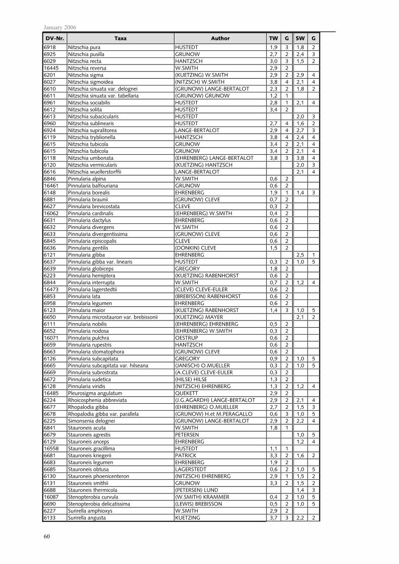
January 2006

60


6918 Nitzschia pura HUSTEDT 1,9 3 1,8 2 6925 Nitzschia pusilla GRUNOW 2,7 2 2,4 3 6029 Nitzschia recta HANTZSCH 3,0 3 1,5 2 16445 Nitzschia reversa W.SMITH 2,9 2 6201 Nitzschia sigma (KUETZING) W.SMITH 2,9 2 2,9 4 6027 Nitzschia sigmoidea (NITZSCH) W.SMITH 3,8 4 2,1 4 6610 Nitzschia sinuata var. delognei (GRUNOW) LANGE-BERTALOT 2,3 2 1,8 2 6611 Nitzschia sinuata var. tabellaria (GRUNOW) GRUNOW 1,2 1 6961 Nitzschia sociabilis HUSTEDT 2,8 1 2,1 4 6612 Nitzschia solita HUSTEDT 3,4 2 6613 Nitzschia subacicularis HUSTEDT 2,0 3 6960 Nitzschia sublinearis HUSTEDT 2,7 4 1,6 2 6924 Nitzschia supralitorea LANGE-BERTALOT 2,9 4 2,7 3 6119 Nitzschia tryblionella HANTZSCH 3,8 4 2,4 4 6615 Nitzschia tubicola GRUNOW 3,4 2 2,1 4 6615 Nitzschia tubicola GRUNOW 3,4 2 2,1 4 6118 Nitzschia umbonata (EHRENBERG) LANGE-BERTALOT 3,8 3 3,8 4 6120 Nitzschia vermicularis (KUETZING) HANTZSCH 2,0 3 6616 Nitzschia wuellerstorffii LANGE-BERTALOT 2,1 4 6846 Pinnularia alpina W.SMITH 0,6 2 16461 Pinnularia balfouriana GRUNOW 0,6 2 6148 Pinnularia borealis EHRENBERG 1,9 1 1,4 3 6881 Pinnularia braunii (GRUNOW) CLEVE 0,7 2 6627 Pinnularia brevicostata CLEVE 0,3 2 16062 Pinnularia cardinalis (EHRENBERG) W.SMITH 0,4 2 6631 Pinnularia dactylus EHRENBERG 0,6 2 6632 Pinnularia divergens W.SMITH 0,6 2 6633 Pinnularia divergentissima (GRUNOW) CLEVE 0,6 2 6845 Pinnularia episcopalis CLEVE 0,6 2 6636 Pinnularia gentilis (DONKIN) CLEVE 1,5 2 6121 Pinnularia gibba EHRENBERG 2,5 1 6637 Pinnularia gibba var. linearis HUSTEDT 0,3 2 1,0 5 6639 Pinnularia globiceps GREGORY 1,8 2 6223 Pinnularia hemiptera (KUETZING) RABENHORST 0,6 2 6844 Pinnularia interrupta W.SMITH 0,7 2 1,2 4 16473 Pinnularia lagerstedtii (CLEVE) CLEVE-EULER 0,6 2 6853 Pinnularia lata (BREBISSON) RABENHORST 0,6 2 6958 Pinnularia legumen EHRENBERG 0,6 2 6123 Pinnularia maior (KUETZING) RABENHORST 1,4 3 1,0 5 6650 Pinnularia microstauron var. brebissonii (KUETZING) MAYER 2,1 2 6111 Pinnularia nobilis (EHRENBERG) EHRENBERG 0,5 2 6652 Pinnularia nodosa (EHRENBERG) W.SMITH 0,3 2 16071 Pinnularia pulchra OESTRUP 0,6 2 6659 Pinnularia rupestris HANTZSCH 0,6 2 6663 Pinnularia stomatophora (GRUNOW) CLEVE 0,6 2 6126 Pinnularia subcapitata GREGORY 0,9 2 1,0 5 6665 Pinnularia subcapitata var. hilseana (JANISCH) O.MUELLER 0,3 2 1,0 5 6669 Pinnularia subrostrata (A.CLEVE) CLEVE-EULER 0,3 2 6672 Pinnularia sudetica (HILSE) HILSE 1,3 2 6128 Pinnularia viridis (NITZSCH) EHRENBERG 1,3 2 1,2 4 16485 Pleurosigma angulatum QUEKETT 2,9 2 6224 Rhoicosphenia abbreviata (J.G.AGARDH) LANGE-BERTALOT 2,9 2 2,1 4 6677 Rhopalodia gibba (EHRENBERG) O.MUELLER 2,7 2 1,5 3 6678 Rhopalodia gibba var. parallela (GRUNOW) H.et M.PERAGALLO 0,6 3 1,0 5 6225 Simonsenia delognei (GRUNOW) LANGE-BERTALOT 2,9 2 2,2 4 6841 Stauroneis acuta W.SMITH 1,8 1 6679 Stauroneis agrestis PETERSEN 1,0 5 6129 Stauroneis anceps EHRENBERG 1,2 4 16558 Stauroneis gracillima HUSTEDT 1,1 1 6681 Stauroneis kriegerii PATRICK 3,3 2 1,6 2 6683 Stauroneis legumen EHRENBERG 1,9 2 6685 Stauroneis obtusa LAGERSTEDT 0,6 2 1,0 5 6130 Stauroneis phoenicenteron (NITZSCH) EHRENBERG 2,9 1 1,5 2 6131 Stauroneis smithii GRUNOW 3,3 2 1,5 2 6688 Stauroneis thermicola (PETERSEN) LUND 1,4 3 16087 Stenopterobia curvula (W.SMITH) KRAMMER 0,4 2 1,0 5 6690 Stenopterobia delicatissima (LEWIS) BREBISSON 0,5 2 1,0 5 6227 Surirella amphioxys W.SMITH 2,9 2 6133 Surirella angusta KUETZING 3,7 3 2,2 2

Janurary 2006

61


6691 Surirella bifrons EHRENBERG 2,3 2 6134 Surirella biseriata BREBISSON 2,1 2 6693 Surirella brebissonii KRAMMER et LANGE-BERTALOT 3,6 5 2,5 2 6994 Surirella capronii BREBISSON 2,5 2 16513 Surirella crumena BREBISSON 2,9 2 6880 Surirella elegans EHRENBERG 2,7 3 6135 Surirella linearis W.SMITH 1,0 2 1,1 4 16091 Surirella linearis var. helvetica (BRUN) MEISTER 0,6 2 1,0 5 6229 Surirella minuta BREBISSON 3,8 3 2,4 3 6136 Surirella ovalis BREBISSON 2,9 4 6694 Surirella roba LECLERCQ 0,6 2 1,0 5 6097 Surirella spiralis KUETZING 0,6 2 16518 Surirella turgida W.SMITH 0,6 2 6074 Tabellaria fenestrata (LYNGBYE) KUETZING 1,4 3 6091 Tabellaria flocculosa (ROTH) KUETZING 0,8 2 1,1 4 6698 Tabellaria ventricosa KUETZING 0,9 2 1,0 5 16522 Tetracyclus glans (EHRENBERG) MILLS 0,6 3 1,0 5 16097 Tetracyclus rupestris (BRAUN) GRUNOW 0,5 2 1,0 5

Table 26: Indicator species for für den salinity of inland waters (modified and continued according to ZIEMANN et al. 1999) HG = Halobic group: hx = haloxenic taxa, hmp = halophilic, mesohalobic and polyhalobic taxa

DV-Nr. Taxa Author HG

6699 Achnanthes altaica (PORETZKY) CLEVE-EULER hx 16105 Achnanthes bahusiensis (GRUNOW) LANGE-BERTALOT hmp 16106 Achnanthes biasolettiana var. subatomus LANGE-BERTALOT hx 16107 Achnanthes brevipes J.G.AGARDH hmp 16528 Achnanthes brevipes var. intermedia (KUETZING) CLEVE hmp 16111 Achnanthes daonensis LANGE-BERTALOT hx 6248 Achnanthes delicatula (KUETZING) GRUNOW hmp 16114 Achnanthes didyma HUSTEDT hx 6253 Achnanthes helvetica (HUSTEDT) LANGE-BERTALOT hx 6256 Achnanthes kranzii LANGE-BERTALOT hx 16119 Achnanthes kuelbsii LANGE-BERTALOT hx 6262 Achnanthes lapidosa KRASSKE hx 6705 Achnanthes laterostrata HUSTEDT hx 6264 Achnanthes levanderi HUSTEDT hx 6045 Achnanthes linearis (W.SMITH) GRUNOW sensu auct. nonnull hx 6265 Achnanthes marginulata GRUNOW hx 6268 Achnanthes oblongella OESTRUP hx 16138 Achnanthes parvula KUETZING hmp 6270 Achnanthes peragalli BRUN & HERIBAUD hx 16139 Achnanthes pseudopunctulata SIMONSEN hmp 16141 Achnanthes punctulata SIMONSEN hmp 6711 Achnanthes rechtensis LECLERCQ hx 16143 Achnanthes rossii HUSTEDT hx 6275 Achnanthes silvahercynia LANGE-BERTALOT hx 6276 Achnanthes subatomoides (HUSTEDT) LANGE-B. & ARCHIBALD hx 6277 Achnanthes suchlandtii HUSTEDT hx 6713 Achnanthes ventralis (KRASSKE) LANGE-BERTALOT hx 6281 Amphipleura rutilans (TRENTEPOHL) CLEVE hmp 16152 Amphora coffeaeformis (J.G.AGARDH) KUETZING hmp 16153 Amphora coffeaeformis var. acutiuscula (KUETZING) RABENHORST hmp 16154 Amphora commutata GRUNOW hmp 16155 Amphora delicatissima KRASSKE hmp 6285 Amphora holsatica HUSTEDT hmp 16156 Amphora lineolata EHRENBERG hmp 16157 Amphora subcapitata (KISSELEV) HUSTEDT hmp 6049 Anomoeoneis sphaerophora (EHRENBERG) PFITZER hmp 6143 Bacillaria paradoxa GMELIN hmp 6291 Brachysira brebissonii ROSS hx 16165 Brachysira follis (EHRENBERG) ROSS hx 16166 Brachysira garrensis (LANGE-B. & KRAMMER) LANGE-B. hx 16167 Brachysira procera LANGE-BERTALOT & MOSER hx 6296 Brachysira serians (BREBISSON) ROUND & MANN hx 16168 Brachysira wygaschii LANGE-BERTALOT hx

January 2006

62


6300 Caloneis aerophila BOCK hx 6043 Caloneis amphisbaena (BORY DE SAINT VINCENT) CLEVE hmp 16171 Caloneis permagna (BAILEY) CLEVE hmp 16172 Caloneis westii (W.SMITH) HENDEY hmp 16174 Campylodiscus clypeus EHRENBERG hmp 16175 Campylodiscus echeneis EHRENBERG hmp 16180 Cocconeis scutellum EHRENBERG hmp 6309 Cylindrotheca gracilis (BREBISSON) GRUNOW hmp 6316 Cymbella descripta (HUSTEDT) KRAMMER & LANGE-B. hx 6317 Cymbella elginensis KRAMMER hx 6319 Cymbella gaeumannii MEISTER hx 6320 Cymbella gracilis (EHRENBERG) KUETZING hx 6321 Cymbella hebridica (GRUNOW) CLEVE hx 6331 Cymbella mesiana CHOLNOKY hx 6747 Cymbella norvegica GRUNOW hx 6977 Cymbella perpusilla CLEVE-EULER hx 6748 Cymbella pusilla GRUNOW hmp 6338 Cymbella stauroneiformis LAGERSTEDT hx 16202 Denticula subtilis GRUNOW hmp 6185 Diatoma anceps (EHRENBERG) KIRCHNER hx 6167 Diatoma hyemalis (ROTH) HEIBERG hx 6949 Diatoma mesodon (EHRENBERG) KUETZING hx 16206 Diatoma moniliformis ssp. ovalis (FRICKE) LANGE-BERTALOT hmp 16207 Diatoma problematica LANGE-BERTALOT hmp 16210 Diploneis didyma (EHRENBERG) EHRENBERG hmp 16211 Diploneis interrupta (KUETZING) CLEVE hmp 16213 Diploneis smithii (BREBISSON) CLEVE hmp 16214 Diploneis smithii var. dilatata (PERAGALLO) TERRY hmp 16215 Diploneis smithii var. pumila (GRUNOW) HUSTEDT hmp 16216 Diploneis smithii var. rhombica MERESCHKOWSKY hmp 16217 Entomoneis alata (EHRENBERG) EHRENBERG hmp 16218 Entomoneis costata (HUSTEDT) REIMER hmp 16219 Entomoneis paludosa (W.SMITH) REIMER hmp 16220 Entomoneis paludosa var. subsalina CLEVE hmp 16221 Eunotia arculus (GRUNOW) LANGE-B. & NOERPEL hx 6886 Eunotia arcus EHRENBERG hx 6213 Eunotia bilunaris (EHRENBERG) MILLS hx 16222 Eunotia bilunaris var. linearis (OKUNO) LANGE-BERTALOT & NOERPEL hx 6355 Eunotia bilunaris var. mucophila LANGE-BERTALOT & NOERPEL hx 6761 Eunotia botuliformis WILD et al. hx 16223 Eunotia circumborealis LANGE-BERTALOT & NOERPEL hx 6356 Eunotia denticulata (BREBISSON) RABENHORST hx 6357 Eunotia diodon EHRENBERG hx 16224 Eunotia elegans OESTRUP hx 6975 Eunotia exigua (BREBISSON) RABENHORST hx 16225 Eunotia exigua var. undulata MAGDEBURG hx 6358 Eunotia faba EHRENBERG hx 6359 Eunotia fallax A.CLEVE hx 6762 Eunotia fallax var. groenlandica (GRUNOW) LANGE-B. & NOERPEL hx 6360 Eunotia flexuosa (BREBISSON) KUETZING hx 6362 Eunotia glacialis MEISTER hx 6363 Eunotia hexaglyphis EHRENBERG hx 6364 Eunotia implicata NOERPEL et al. hx 6214 Eunotia incisa GREGORY hx 6365 Eunotia intermedia (KRASSKE) NOERPEL & LANGE-B. hx 16226 Eunotia islandica OESTRUP hx 16104 Eunotia jemtlandica (FONTELL) BERG hx 16228 Eunotia major (W.SMITH) RABENHORST hx 6367 Eunotia meisteri HUSTEDT hx 6368 Eunotia microcephala KRASSKE hx 6885 Eunotia monodon EHRENBERG hx 6370 Eunotia muscicola var. tridentula NOERPEL & LANGE-BERTALOT hx 6371 Eunotia naegelii MIGULA hx 16695 Eunotia neofallax NOERPEL hx 6372 Eunotia nymanniana GRUNOW hx 6373 Eunotia paludosa GRUNOW hx 6884 Eunotia paludosa var. trinacria (KRASSKE) NOERPEL hx 6168 Eunotia pectinalis (DILLWYN) RABENHORST hx 6766 Eunotia pectinalis var. undulata (RALFS) RABENHORST hx 6851 Eunotia praerupta EHRENBERG hx

Janurary 2006

63


6767 Eunotia praerupta var. bidens (EHRENBERG) GRUNOW hx 6374 Eunotia praerupta var. bigibba (KUETZING) GRUNOW hx 6768 Eunotia praerupta var. curta GRUNOW hx 6769 Eunotia praerupta var. inflata GRUNOW hx 16229 Eunotia pseudopectinalis HUSTEDT hx 6375 Eunotia rhomboidea HUSTEDT hx 16230 Eunotia rhynchocephala HUSTEDT hx 6376 Eunotia septentrionalis OESTRUP hx 6850 Eunotia serra EHRENBERG hx 6770 Eunotia serra var. diadema (EHRENBERG) PATRICK hx 6377 Eunotia serra var. tetraodon (EHRENBERG) NOERPEL hx 6378 Eunotia silvahercynia NOERPEL et al. hx 6379 Eunotia soleirolii (KUETZING) RABENHORST hx 6380 Eunotia steineckei PETERSEN hx 6381 Eunotia subarcuatoides ALLES et al. hx 6382 Eunotia sudetica O.MUELLER hx 6383 Eunotia tenella (GRUNOW) HUSTEDT hx 16668 Eunotia tetraodon EHRENBERG hx 6771 Eunotia triodon EHRENBERG hx 16233 Fragilaria acidoclinata LANGE-BERTALOT & HOFMANN hx 16234 Fragilaria constricta EHRENBERG hx 6401 Fragilaria exigua GRUNOW hx 6234 Fragilaria fasciculata (J.G.AGARDH) LANGE-BERTALOT hmp 6238 Fragilaria pulchella (RALFS) LANGE-BERTALOT hmp 6169 Fragilaria virescens RALFS hx 16245 Frustulia creuzburgensis (KRASSKE) HUSTEDT hmp 6187 Frustulia rhomboides (EHRENBERG) DE TONI hx 6412 Frustulia rhomboides var. crassinervia (BREBISSON) ROSS hx 6413 Frustulia rhomboides var. saxonica (RABENHORST) DE TONI hx 6414 Frustulia rhomboides var. viridula (BREBISSON) CLEVE hx 6421 Gomphonema bohemicum REICHELT & FRICKE hx 6424 Gomphonema hebridense GREGORY hx 6426 Gomphonema lagerheimii A.CLEVE hx 6430 Gomphonema olivaceum var. minutissimum HUSTEDT hx 6435 Gomphonema productum (GRUNOW) LANGE-B. & REICHARDT hx 6999 Gomphonema ventricosum GREGORY hx 16227 Gyrosigma balticum (EHRENBERG) RABENHORST hmp 16262 Gyrosigma parkeri (HARRISON) ELMORE hmp 6996 Gyrosigma peisonis (GRUNOW) HUSTEDT hmp 6042 Gyrosigma spenceri (W.SMITH) CLEVE hmp 16263 Gyrosigma strigilis W.SMITH hmp 16270 Hantzschia spectabilis (EHRENBERG) HUSTEDT hmp 16272 Hantzschia virgata (ROPER) GRUNOW hmp 16277 Hantzschia vivax (W.SMITH) M.PERAGALLO hmp 16279 Mastogloia baltica GRUNOW hmp 16280 Mastogloia braunii GRUNOW hmp 16281 Mastogloia elliptica J.G.AGARDH hmp 6803 Mastogloia elliptica var. dansei (THWAITES) CLEVE hmp 6444 Mastogloia smithii THWAITES hmp 16287 Melosira nummuloides (DILLWYN) J.G.AGARDH hmp 6446 Meridion circulare var. constrictum (RALFS) VAN HEURCK hx 16717 Navicula adversa KRASSKE hx 6809 Navicula angusta GRUNOW hx 16290 Navicula arenaria DONKIN hmp 16297 Navicula bulnheimii GRUNOW hmp 6089 Navicula cincta (EHRENBERG) RALFS hmp 6969 Navicula cocconeiformis GREGORY hx 6901 Navicula crucicula (W.SMITH) DONKIN hmp 16304 Navicula crucigera (W.SMITH) CLEVE hmp 16306 Navicula cryptolyra BROCKMANN hmp 6038 Navicula cuspidata (KUETZING) KUETZING hmp 6475 Navicula detenta HUSTEDT hx 6477 Navicula digitoradiata (GREGORY) RALFS hmp 16000 Navicula digitulus HUSTEDT hx 6479 Navicula duerrenbergiana HUSTEDT hmp 16314 Navicula elegans W.SMITH hmp 6482 Navicula evanida HUSTEDT hx 6917 Navicula exilis KUETZING hx 16316 Navicula flanatica GRUNOW hmp 6489 Navicula gallica var. perpusilla (GRUNOW) LANGE-BERTALOT hx

January 2006

64


6833 Navicula halophila (GRUNOW) CLEVE hmp 16321 Navicula halophiloides HUSTEDT hmp 6496 Navicula heimansioides LANGE-BERTALOT hx 16325 Navicula humerosa BREBISSON hmp 6812 Navicula integra (W.SMITH) RALFS hmp 6509 Navicula krasskei HUSTEDT hx 16010 Navicula lapidosa KRASSKE hx 16011 Navicula leptostriata JOERGENSEN hx 16337 Navicula levanderii HUSTEDT hx 6513 Navicula mediocris KRASSKE hx 16346 Navicula microdigitoradiata LANGE-BERTALOT hmp 16349 Navicula notha WALLACE hx 6098 Navicula peregrina (EHRENBERG) KUETZING hmp 16353 Navicula perminuta GRUNOW hmp 6866 Navicula phyllepta KUETZING hmp 16355 Navicula plicata DONKIN hmp 6100 Navicula protracta (GRUNOW) CLEVE hmp 6527 Navicula pseudobryophila (HUSTEDT) HUSTEDT hx 6102 Navicula pygmaea KUETZING hmp 6534 Navicula recens (LANGE-BERTALOT) LANGE-BERTALOT hmp 16362 Navicula rhynchotella LANGE-BERTALOT hmp 6105 Navicula salinarum GRUNOW hmp 16365 Navicula salinicola HUSTEDT hmp 6539 Navicula schmassmannii HUSTEDT hx 6540 Navicula schroeterii MEISTER hmp 6543 Navicula soehrensis KRASSKE hx 16034 Navicula soehrensis var. hassiaca (KRASSKE) LANGE-BERTALOT hx 6544 Navicula soehrensis var. muscicola (PETERSEN) KRASSKE hx 16370 Navicula soodensis KRASSKE hmp 16371 Navicula spicula (HICKIE) CLEVE hmp 6549 Navicula submolesta HUSTEDT hx 6878 Navicula subtilissima CLEVE hx 6551 Navicula suchlandtii HUSTEDT hx 16376 Navicula tenera HUSTEDT hmp 16037 Navicula variostriata KRASSKE hx 6563 Neidium alpinum HUSTEDT hx 6566 Neidium bisulcatum (LAGERSTEDT) CLEVE hx 6110 Neidium productum (W.SMITH) CLEVE hx 6573 Nitzschia acidoclinata LANGE-BERTALOT hx 16390 Nitzschia agnita HUSTEDT hmp 6575 Nitzschia alpina HUSTEDT hx 16391 Nitzschia amplectens HUSTEDT hmp 6580 Nitzschia brevissima GRUNOW hmp 16048 Nitzschia calida GRUNOW hmp 16397 Nitzschia circumsuta (BAILEY) GRUNOW hmp 6193 Nitzschia clausii HANTZSCH hmp 6581 Nitzschia commutata GRUNOW hmp 6583 Nitzschia compressa var. balatonis (GRUNOW) LANGE-BERTALOT hmp 16049 Nitzschia compressa var. vexans (GRUNOW) LANGE-BERTALOT hmp 6242 Nitzschia constricta (KUETZING) RALFS hmp 16402 Nitzschia dippelii GRUNOW hmp 6113 Nitzschia dubia W.SMITH hmp 16405 Nitzschia elegantula GRUNOW hmp 16406 Nitzschia epithemoides GRUNOW hmp 16408 Nitzschia fasciculata GRUNOW hmp 6195 Nitzschia filiformis (W.SMITH) VAN HEURCK hmp 6196 Nitzschia frustulum (KUETZING) GRUNOW hmp 6591 Nitzschia frustulum var. bulnheimiana (RABENHORST) GRUNOW hmp 6931 Nitzschia hantzschiana RABENHORST hx 16051 Nitzschia homburgiensis LANGE-BERTALOT hx 6114 Nitzschia hungarica GRUNOW hmp 16414 Nitzschia hybrida GRUNOW hmp 6595 Nitzschia inconspicua GRUNOW hmp 6888 Nitzschia levidensis (W.SMITH) GRUNOW hmp 16102 Nitzschia levidensis var. salinarum GRUNOW hmp 16052 Nitzschia levidensis var. victoriae GRUNOW hmp 16423 Nitzschia liebetruthii RABENHORST hmp 6601 Nitzschia littoralis GRUNOW hmp 16427 Nitzschia lorenziana GRUNOW hmp 6198 Nitzschia microcephala GRUNOW hmp

Janurary 2006

65


16055 Nitzschia obtusa W.SMITH hmp 6602 Nitzschia ovalis ARNOTT hmp 16437 Nitzschia perspicua CHOLNOKY hmp 16446 Nitzschia rosenstockii LANGE-BERTALOT hmp 16447 Nitzschia scalaris (EHRENBERG) W.SMITH hmp 16057 Nitzschia scalpelliformis (GRUNOW) GRUNOW hmp 6201 Nitzschia sigma (KUETZING) W.SMITH hmp 6119 Nitzschia tryblionella HANTZSCH hmp 16058 Nitzschia vitrea NORMAN hmp 6619 Peronia fibula (BREBISSON) ROSS hx 6621 Pinnularia anglica KRAMMER hx 6622 Pinnularia angusta (CLEVE) KRAMMER hx 6623 Pinnularia appendiculata (J.G.AGARDH) CLEVE hmp 16543 Pinnularia bacilliformis KRAMMER hx 6625 Pinnularia brandelii CLEVE hx 16463 Pinnularia brauniana (GRUNOW) MILLS hx 6627 Pinnularia brevicostata CLEVE hx 16062 Pinnularia cardinalis (EHRENBERG) W.SMITH hx 6629 Pinnularia cleveiformis KRAMMER hx 6845 Pinnularia episcopalis CLEVE hx 6636 Pinnularia gentilis (DONKIN) CLEVE hx 16065 Pinnularia gigas EHRENBERG hx 6125 Pinnularia microstauron (EHRENBERG) CLEVE hx 6651 Pinnularia neomajor KRAMMER hx 6658 Pinnularia pseudogibba KRAMMER hx 6659 Pinnularia rupestris HANTZSCH hx 6660 Pinnularia schoenfelderi KRAMMER hx 16074 Pinnularia silvatica PETERSEN hx 6663 Pinnularia stomatophora (GRUNOW) CLEVE hx 16479 Pinnularia stomatophora var. triundulata (FONTELL) HUSTEDT hx 6664 Pinnularia streptoraphe CLEVE hx 16480 Pinnularia streptoraphe var. parva KRAMMER hx 6126 Pinnularia subcapitata GREGORY hx 16481 Pinnularia subcapitata var. elongata KRAMMER hx 6665 Pinnularia subcapitata var. hilseana (JANISCH) O.MUELLER hx 6670 Pinnularia subrupestris KRAMMER hx 16485 Pleurosigma angulatum QUEKETT hmp 16486 Pleurosigma elongatum W.SMITH hmp 16078 Pleurosigma salinarum GRUNOW hmp 16487 Pleurosira laevis (EHRENBERG) COMPERE hmp 16492 Rhopalodia constricta (W.SMITH) KRAMMER hmp 6677 Rhopalodia gibba (EHRENBERG) O.MUELLER hmp 16493 Rhopalodia musculus (KUETZING) O.MUELLER hmp 6840 Stauroneis nobilis SCHUMANN hx 16501 Stauroneis salina W.SMITH hmp - Stauroneis simulans (DONKIN) ROSS hmp 16087 Stenopterobia curvula (W.SMITH) KRAMMER hx 6690 Stenopterobia delicatissima (LEWIS) BREBISSON hx 16503 Stenopterobia densestriata (HUSTEDT) KRAMMER hx 16510 Surirella brightwellii W.SMITH hmp 16511 Surirella brightwellii var. baltica (SCHUMANN) KRAMMER hmp 16513 Surirella crumena BREBISSON hmp 6136 Surirella ovalis BREBISSON hmp 6694 Surirella roba LECLERCQ hx 16517 Surirella striatula TURPIN hmp 16519 Tabellaria binalis (EHRENBERG) GRUNOW hx 16520 Tabellaria binalis var. elliptica FLOWER hx 16096 Tabellaria quadriseptata KNUDSON hx 6698 Tabellaria ventricosa KUETZING hx

January 2006

66

4.3 Phytobenthos without diatoms For phytobenthos evaluation indicative species of comparable ecological conditions are summed up in the classification categories A, B, C and D (Table 27). This category must be noted for each taxon of a sampling site. It must be kept in mind that classification of taxa into different categories can vary between the different groups of running waters.

For calculation of the Assessment Index quantities must be squared. The Assessment index is calculated according to equation 15. Theoretically the calculated value can lie between +100 and –100.

Calculation of the Assessment Index can be considered reliable, if at least five indicative taxa were found or if (in case of less than 5 taxa) the sum of the squared degrees of cover adds up to more than 16. If an assessment is not reliable this must be noted. For running water sampling sites of the Alps and the Alpine Foreland presently no assessment procedure is available

Equation 15: Calculation of the Assessment Index

100*21

21

1 1 1 1

1 1 1 1

∑ ∑ ∑ ∑

∑ ∑ ∑ ∑

= = = =

= = = =

+++

−−+=

A B C D

A B C D

n

i

n

i

n

i

n

iDiCiBiAi

n

i

n

i

n

i

n

iDiCiBiAi

QQQQ

QQQQBI

BI =Assessment Iindex QA = squared quantity of a taxon from assessment category A QB = suared quantity of a taxon from assessment category B QC = squared quantity of a taxon from assessment category C QD = suared quantity of a taxon from assessment category D i = 1 to nA, nB, nC, nD

Table 27: List of indicators in the submodule Phytobenthos without Diatoms MG_sil = running waters of the Central German Uplands with siliceous influence, MG_karb = running waters of the Central German Uplands with calcareous influence, NT_karb =running waters of the North German Lowland with calcareous influence, NT_sil/org = running waters of the North German Lowland with siliceous and organic influence.

System Name MG_sil MG_cal NT_cal NT_sil/org

Nostocophyceae Aphanocapsa fonticola A B Nostocophyceae Aphanocapsa rivularis A Nostocophyceae Aphanothece stagnina C B C Nostocophyceae Chamaesiphon confervicolus B B Nostocophyceae Chamaesiphon fuscus A Nostocophyceae Chamaesiphon incrustans B B B B Nostocophyceae Chamaesiphon polonicus B Nostocophyceae Chamaesiphon polymorphus C C Nostocophyceae Chamaesiphon starmachii A Nostocophyceae Chamaesiphon subglobosus B A A Nostocophyceae Chroococcopsis gigantea B B B Nostocophyceae Heteroleibleinia kuetzingii B B Nostocophyceae Homoeothrix crustacea A Nostocophyceae Homoeothrix janthina A C A Nostocophyceae Homoeothrix varians B B B B Nostocophyceae Hydrococcus cesatii B A Nostocophyceae Hydrococcus rivularis B A Nostocophyceae Hyella fontana A Nostocophyceae Komvophoron constrictum C C C Nostocophyceae Leptolyngbya foveolarum D D D Nostocophyceae Merismopedia glauca A A Nostocophyceae Microcoleus vaginatus C Nostocophyceae Nostoc parmelioides A Nostocophyceae Oscillatoria limosa C C C C Nostocophyceae Oscillatoria princeps C

Janurary 2006

67


Nostocophyceae Phormidium ambiguum C Nostocophyceae Phormidium corium B A A Nostocophyceae Phormidium incrustatum C A A Nostocophyceae Phormidium retzii C C C C Nostocophyceae Phormidium subfuscum B C C Nostocophyceae Plectonema tomasinianum B Nostocophyceae Pleurocapsa minor C C Nostocophyceae Porphyrosiphon martensianus B Nostocophyceae Pseudanabaena catenata D Nostocophyceae Schizothrix tinctoria B Nostocophyceae Xenotholos kerneri A Bangiophyceae Bangia atropurpurea B B B Florideophyceae Audouinella B A A B Florideophyceae Audouinella chalybaea B A A B Florideophyceae Audouinella hermannii B A A B Florideophyceae Audouinella pygmaea B A A B Florideophyceae Batrachospermum B B B B Florideophyceae Batrachospermum gelatinosum B B B Florideophyceae Batrachospermum helminthosum A Florideophyceae Chantransia - Stadien B B B B Florideophyceae Hildenbrandia rivularis B B B Florideophyceae Lemanea B Florideophyceae Lemanea fluviatilis A B Florideophyceae Paralemanea B Florideophyceae Thorea sp. A Fucophyceae Heribaudiella fluviatilis B B Chrysophyceae Hydrurus foetidus B Chrysophyceae Phaeodermatium rivulare B B Euglenophyceae Lepocinclis texta B Euglenophyceae Phacus acuminatus B Euglenophyceae Phacus orbicularis B Tribophyceae Tribonema viride C B C Tribophyceae Tribonema vulgare B B Tribophyceae Vaucheria C C B C Tribophyceae Vaucheria mit Häufigkeit 5 C Chlorophyceae Bulbochaete B Chlorophyceae Draparnaldia mutabilis B Chlorophyceae Gongrosira debaryana B B B Chlorophyceae Gongrosira fluminensis B Chlorophyceae Gongrosira incrustans A A Chlorophyceae Microspora B B B Chlorophyceae Microspora amoena B B B B Chlorophyceae Microspora floccosa B B B B Chlorophyceae Microspora stagnorum B B Chlorophyceae Microspora tumidulum B B Chlorophyceae Microspora wittrockii B B B Chlorophyceae Oedogonium B C C B Chlorophyceae Oedogonium mit Häufigkeit 5 C C Chlorophyceae Stigeoclonium D D D D Chlorophyceae Stigeoclonium farctum D Chlorophyceae Tetraspora gelatinosa A A A A Trebouxiophyceae Microthamnion curvatum B C Trebouxiophyceae Microthamnion kuetzingianum B C Trebouxiophyceae Microthamnion strictissimum B C Ulvophyceae Cladophora glomerata C B B C Ulvophyceae Cladophora glomerata mit Häufigkeit 5 C C Ulvophyceae Cladophora rivularis B B C Ulvophyceae Cladophora rivularis mit Häufigkeit 5 C C Ulvophyceae Enteromorpha C C Ulvophyceae Enteromorpha prolifera D D Ulvophyceae Rhizoclonium hieroglyphicum C C C C Ulvophyceae Ulothrix tenerrima C C C Ulvophyceae Ulothrix tenuissima B B B

January 2006

68


Ulvophyceae Ulothrix zonata B B B Charophyceae Actinotaenium cruciferum A Charophyceae Closterium acerosum C C C C Charophyceae Closterium cornu A Charophyceae Closterium dianae A Charophyceae Closterium eboracense - B Charophyceae Closterium ehrenbergii C B B C Charophyceae Closterium ehrenbergii var. malinverianum C Charophyceae Closterium incurvum B B Charophyceae Closterium intermedium A Charophyceae Closterium kuetzingii B C Charophyceae Closterium leibleinii var. boergensenii C B B C Charophyceae Closterium littorale B B Charophyceae Closterium littorale var. crassum C B B Charophyceae Closterium moniliferum C B B C Charophyceae Closterium moniliferum var. concavum C B B Charophyceae Closterium nilssonii A Charophyceae Closterium praelongum Charophyceae Closterium praelongum var. brevius B B B B Charophyceae Closterium rostratum A C C A Charophyceae Closterium strigosum B B B B Charophyceae Closterium strigosum var. elegans B B B B Charophyceae Closterium striolatum A A Charophyceae Closterium sublaterale C B B C Charophyceae Closterium tumidulum B B B B Charophyceae Closterium tumidum A Charophyceae Cosmarium laeve C C C Charophyceae Cosmarium pachydermum var. aetiopicum A Charophyceae Klebsormidium rivulare A Charophyceae Mougeotia B B B B Charophyceae Penium margaritaceum A Charophyceae Pleurotaenium crenulatum A Charophyceae Spirogyra B B B B Charophyceae Staurastrum punctulatum B Charophyceae Xanthidium antilopaeum A Charophyceae Zygnema B

Janurary 2006

69

4.4 Overall assessment of running waters with Macrophytes & Phytobenthos

According to the WFD the entire group of organisms consisting of the benthic flora, Macrophytes & Phytobenthos is considered to be one of the four biological components to assess the status of a water system. Therefore, the three subcomponents must be considered as modules or metrics for assessment in terms of the WFD.

4.4.1 Combination of the metrics Macrophytes, Diatoms and Phytobenthos without Diatoms

For the overall assessment of running waters with the biocomponent Macrophytes & Phytobenthos it is absolutely necessary to carry out an assessment of the three subcomponents Macrophytes, Diatoms and Phytobenthos without Diatoms exactly following the method described for these modules. A prerequisite is the collection of data according to the guidelines and exact determination of the biocoenotic type depending on different groups of organisms. In particular cases there are contradictory results for the different sub-groups of organisms. A sampling site can be attributed to the siliceous type of running water according to LAWA, but can be influenced by calcareous water from the catchment area. It is possible to have an attribution to a siliceous diatom type and a calcareous macrophyte type or phytobenthos type. In such cases it must be verified, if the increased values for hardness or acid capacity are the result of anthropogenic influences as for example the discharge of industrial waste. The values are then considered the result of degradation and the type must be corrected correspondingly. This situation can often be observed for strongly degraded waters as well as for waters with a large catchment area. If a sampling section is located in an area of alternating geological conditions, if possible, a geologically more homogenous site should be chosen.

The combination of calcareous geology and low hardness is impossible.

The differentiation between rhitral or potamal running waters according to the macrophyte typology is important for the chances of higher water plants to colonise this type of water. Mechanical stress exerted on the plants due to the continuous flow and the resistance of the individual species towards this kind of stress plays an important role. In contrast to certain types of small, narrow leafed species of Potamogeton for example, a large leafed species will hardly be expected in turbulently running waters. In its natural state, a running water with a large catchment area can for certain stretches show water levels and velocities of flow that are only suitable for species resistant to the current.

The LAWA typology or type map, which nationwide is in effect, cannot yet exclusively be used as the sole basis for type determination. Typology of the macrophyte and phytobenthos assessment procedure can easily be harmonised with this system (SCHAUMBURG et al. 2005, as well as chapter 3), but as the nationwide type map is still being worked upon and as after completion of other biological projects there might still be changes, typification of the sampling sites according to the

January 2006

70

described criteria is necessary. Furthermore, the changes in type attribution show that nationwide type attribution cannot be considered completed.

In order to create a basis for comparison for the three metrics Macrophytes, Diatoms and Phytobenthos without Diatoms, all index values must be transformed to match a unified scale from “0“ to “1“. The value „1“ reflects the best possible ecological status in terms of the WFD, i.e. ecological status class 1. A value of “0” stands for the highest degree of degradation of a water system, i.e. ecological status class 5. Transformation of the module “Macrophytes” (Reference Index, RI) and the module “Phytobenthos without Diatoms” (Assessment Index, BI) is carried out following Equation 16 and Equation 17. The result of the module “Diatoms” (Diatom IndexFließgewässer = DIFG) already is on this scale and therefore does not need to be transformed.

Equation 16: Equation for transformation of the module RIFG (Reference IndexFließgewässer macrophytes) on a scale from 0 to 1.

1005,0*)100( +

= FGMP

RIM

MMP = Module Macrophyte Assessment RIFG = type specifically calculated reference index

Equation 17: Equation for transformation of the module BI (Assessment Index Phytobenthos without Diatoms) on a scale from 0 to 1

1005,0*)100( +

=BIM PB

MPB = Module Phytobenthos BI = type specific assessment index

Calculation of the common Macrophyte-Phytobenthos Index of running waters (M& PFG ) from the three components is carried out according to Equation 18. If individual modules cannot be considered reliable, the Macrophyte Phytobenthos Index for running waters M& PFG can be calculated in addition. If the module “Macrophytes” is not reliable, Equation 19 is used and if the module “Phytobenthos without Diatoms” is not reliable Equation 20. If, in exceptional cases the module “Diatoms” cannot reliably be evaluated, Equation 21 can be referred to. If two modules are inconclusive, assessment is done according to the one reliable module. Nevertheless, the final result must be critically verified and doesn’t have the same significance as an assessment with two or three modules!

Equation 18: Calculation of the index value M&PFG for determination of the ecological status class of a running water system in case of three reliable modules.

3& MMMPM PBDMPFG

++=

M&PFG = Macrophyte & Phytobenthos-Index for running waters

MMP = Module Macrophytes MD = Module Diatoms MPB = Module Phytobenthos without Diatoms

Equation 19: Calculation of the index value M&PFG for determination of the ecological status class of a running water if the modules Diatoms and Phytobenthos without Diatoms are reliable.

2& MMPM PBDFG

+=

M&PFG = Macrophytes & Phytobenthos-Index for running waters

MD = Module Diatoms MPB = Module Phytobenthos without Diatoms

Janurary 2006

71

Equation 20: Calculation of the index value M&PFG for determination of the ecological status class of a running water, if the modules Macrophytes and Diatoms are reliable.

2& MMPM DMPFG

+=


MMP = Module Macrophytes MD = Module Diatoms

Equation 21: Calculation of the index value M&PFG for determination of the ecological status class in case the module Macrophytes and the module Phytobenthos without Diatoms are reliable.

2& MMPM PBMPFG

+=


MPB = Module Phytobenthos without Diatoms MMP = Module Macrophytes

4.4.2 Determination of the ecological status class

Separated according to ecoregions Table 28to Table 71show the limits for attribution of the calculated index M&PFG to the ecological status classes according to the WFD. If one or two modules must be considered inconclusive, the results will still be used as a aid for interpretation of the total result, but will not be used for classification of the ecological status according to the WFD. An exception is the designation of an unreliable status class 5 in the sub module Macrophytes, which in case of a proven macrophyte depopulation (e.g. due to mowing, clearing, high input of nutrients, introduction of herbivorous fish) is assigned. In this case, if the ecological status “good” or “high” is determined with the module Diatoms and Phytobenthos, the ecological status class “moderate” (3) is assigned.

For unreliable individual assessments the index limits are also listed in the tables mentioned above.

.

January 2006

72

4.4.2.1 Alps

As due to a lack of data for the ecoregion Alps no assessment procedure for the module “Phytobenthos without Diatoms” could be developed, assessment of these sampling sites is carried out pursuant to the WFD with the modules “Macrophytes” and “Diatoms”.

Assessment with the modules Macrophytes and Diatoms

Table 28: Index limits for attribution of the ecological status class: Running waters of the calcareous alps with a catchment area of 1000 km²

Diatoms D 1.1

Running waters of the calcareous alps with a catchment area < 1000 km2

Macrophytes MRK MP MPG

1 1,00 – 0,67 1,00 – 0,75 1,00 – 0,80

2 0,66 – 0,52 0,74 – 0,45 0,79 – 0,52

3 0,51 – 0,26 0,44 – 0,21 0,51 – 0,28

4 0,25 – 0,00 0,20 – 0,00 0,27 – 0,00

5 – – –

Table 29: Index limits for attribution of the ecological status class: Running waters of the calcareous alps with a catchment area larger than1000 km²

Diatoms D 1.2

Running waters of the calcareous alps with a catchment area > 1000 km2


1 1,00 – 0,65 1,00 – 0,73 1,00 – 0,78

2 0,64 – 0,50 0,72 – 0,42 0,77 – 0,50

3 0,49 – 0,26 0,41 – 0,21 0,49 – 0,28

4 0,25 – 0,00 0,20 – 0,00 0,27 – 0,00

5 – – –

Janurary 2006

73

Assessment with the module Diatoms to be applied, if the module Macrophytes is not reliable

Table 30: Index limits for attribution of the ecological status class if the module Macrophytes is not reliable: Running waters of the calcareous alps

Diatoms

D 1.1 Running waters of the calcareous alps with a catchment

area < 1000 km2

D 1.2 Running waters of the calcareous alps with a catchment

area > 1000 km2

1 1,00 – 0,74 1,00 – 0,71

2 0,73 – 0,54 0,70 – 0,49

3 0,53 – 0,31 0,48 – 0,31

4 0,30 – 0,08 0,30 – 0,08

5 0,07 – 0,00 0,07 – 0,00

Assessment with the module Macrophytes to be applied, if the module Diatoms is not reliable

Table 31: Index limits for attribution of the ecological status class, if the module Diatoms is not reliable: Running waters of the calcareous alps


1 1,00 – 0,59 1,00 – 0,75 1,00 – 0,85

2 0,58 – 0,50 0,74 – 0,35 0,84 – 0,50

3 0,49 – 0,20 0,34 – 0,10 0,49 – 0,25

4 0,19 – 0,00 0,09 – 0,00 0,24 – 0,00

5 – – –

January 2006

74

4.4.2.2 Alpine Foreland

Due to a lack of data for the running water systems of the Alpine Foreland no assessment procedure could be developed for the module “Phytobenthos without Diatoms“. As a consequence the assessment according to the WFD is carried out with the module “Macrophytes“ and the module “Diatoms“.

Assessment with the modules Macrophytes and Diatoms

Table 32: Index limits for attribution of the ecological status class: Siliceous running waters of the Alpine Foreland with a catchment area smaller than 1000 km²

Diatoms D 2 Siliceous running waters with a catchment area < 1000 km2

Macrophytes MRK MP MPG MRS

1 1,00 – 0,63 1,00 – 0,71 1,00 – 0,76 1,00 – 0,71

2 0,62 – 0,47 0,70 – 0,39 0,75 – 0,47 0,70 – 0,47

3 0,46 – 0,22 0,38 – 0,17 0,46 – 0,25 0,46 – 0,25

4 0,21 – 0,00 0,16 – 0,00 0,24 – 0,00 0,24 – 0,00

5 – – – –

Table 33: Index limits for attribution of the ecological status class: Calcareous running waters of the Alpine Foreland with a catchment area smaller than 1000 km²

Diatoms D 3 Calcareous running waters with a catchment area < 1000 km2


1 1,00 – 0,63 1,00 – 0,71 1,00 – 0,76 1,00 – 0,71

2 0,62 – 0,47 0,70 – 0,39 0,75 – 0,47 0,70 – 0,47

3 0,46 – 0,22 0,38 – 0,17 0,46 – 0,25 0,46 – 0,25

4 0,21 – 0,00 0,16 – 0,00 0,24 – 0,00 0,24 – 0,00

5 – – – –

Table 34: Index limits for attribution of the ecological status class: Running waters of the Alpine Foreland with a catchment area larger than 1000 km²

Diatoms D 4 Running waters with a catchment area > 1000 km2


1 1,00 – 0,60 1,00 – 0,68 1,00 – 0,73 1,00 – 0,68

2 0,59 – 0,47 0,67 – 0,39 0,72 – 0,47 0,67 – 0,47

3 0,46 – 0,22 0,38 – 0,17 0,46 – 0,25 0,46 – 0,25

4 0,21 – 0,00 0,16 – 0,00 0,24 – 0,00 0,24 – 0,00

5 – – – –

Janurary 2006

75

Assessment with the module Diatoms to be applied, if the module Macrophytes is not reliable

Table 35: Index limits for attribution of the ecological status class to be applied, if the module Macrophytes is not reliable: Running waters of the Alpine Foreland

Diatoms

D 2 Siliceous running

waters with a catchment area

< 1000 km2

D 3 Calcareous running


< 1000 km2

D 4 Running waters

with a catchment area

> 1000 km2

1 1,00 – 0,67 1,00 – 0,67 1,00 – 0,61

2 0,66 – 0,43 0,66 – 0,43 0,60 – 0,43

3 0,42 – 0,24 0,42 – 0,24 0,42 – 0,24

4 0,23 – 0,08 0,23 – 0,08 0,23 – 0,08

5 0,07 – 0,00 0,07 – 0,00 0,07 – 0,00

Assessment with the module Macrophytes to be applied, if the module Diatoms is not reliable

Table 36: Index limits for attribution of the ecological status class to be applied, if the module Diatoms is not reliable: Running waters of the Alpine Foreland


1 1,00 – 0,59 1,00 – 0,75 1,00 – 0,85 1,00 – 0,75

2 0,58 – 0,50 0,74 – 0,35 0,84 – 0,50 0,74 – 0,51

3 0,49 – 0,20 0,34 – 0,10 0,49 – 0,25 0,50 – 0,25

4 0,19 – 0,00 0,09 – 0,00 0,24 – 0,00 0,24 – 0,00

5 – – – –

January 2006

76

4.4.2.3 Central German Upland

Assessment with the modules Macrophytes, Diatoms and Phytobenthos without Diatoms

Table 37: Index limits for attribution of the ecological status class: Siliceous running waters of the variegated sandstone and the bedrock of the Central German Uplands with a catchment area smaller than 100 km²

Phytobenthos MG_sil

Diatoms D 5

Running waters of the variegated sandstone and the bedrock with a catchment area < 100 km2


1 1,00 – 0,67 1,00 – 0,72 1,00 – 0,76 1,00 – 0,72

2 0,66 – 0,51 0,71 – 0,46 0,75 – 0,51 0,72 – 0,51

3 0,50 – 0,28 0,45 – 0,25 0,50 – 0,30 0,51 – 0,30

4 0,27 – 0,00 0,24 – 0,00 0,29 – 0,00 0,29 – 0,00

5 – – – –

Table 38: Index limits for attribution of the ecological status class: Siliceous running waters of volcanic areas in the Central German Uplands with a catchment area smaller than 100 km²

Phytobenthos MG_sil

Diatoms D 6 Running waters of volcanic areas with a catchment area < 100 km2


1 1,00 – 0,65 1,00 – 0,70 1,00 – 0,74 1,00 – 0,70

2 0,64 – 0,50 0,69 – 0,45 0,73 – 0,50 0,69 – 0,50

3 0,49 – 0,28 0,44 – 0,25 0,49 – 0,30 0,49 – 0,30

4 0,27 – 0,00 0,24 – 0,00 0,29 – 0,00 0,29 – 0,00

5 – – – –

Table 39: Index limits for attribution of the ecological status class: Siliceous running waters of the variegated sandstone and bedrock of the Central German Uplands with a catchment area larger than 100 km² and smaller than 1000 km²

Phytobenthos MG_sil

Diatoms D 7

Running waters of the variegated sandstone and bedrock with a catchment area > 100 km2 and < 1000 km2


1 1,00 – 0,65 1,00 – 0,70 1,00 – 0,74 1,00 – 0,70

2 0,64 – 0,50 0,69 – 0,45 0,73 – 0,50 0,69 – 0,50

3 0,49 – 0,28 0,44 – 0,25 0,49 – 0,30 0,49 – 0,30

4 0,27 – 0,00 0,24 – 0,00 0,29 – 0,00 0,29 – 0,00

5 – – – –

Janurary 2006

77

Table 40: Index limits for attribution of the ecological status class: Calcareous running waters of the loess- and keuper regions of the Central German Uplands with a catchment area smaller than 1000 km²

Phytobenthos MG_calc

Diatoms D 8 Running waters of the loess and keuper regions with a catchment area ≤ 1000 km2


1 1,00 – 0,63 1,00 – 0,69 1,00 – 0,72 1,00 – 0,69

2 0,62 – 0,50 0,68 – 0,45 0,71 – 0,50 0,68 – 0,50

3 0,49 – 0,28 0,44 – 0,25 0,49 – 0,30 0,49 – 0,30

4 0,27 – 0,00 0,24 – 0,00 0,29 – 0,00 0,29 – 0,00

5 – – – –

Table 41: Index limits for attribution of the ecological status class: Calcareous running water of calcareous regions in the Central German Uplands with a catchment area smaller than 100 km²


Diatoms D 9.1

Running waters of calcareous regions with a catchment area ≤ 100 km2


1 1,00 – 0,65 1,00 – 0,70 1,00 – 0,74 1,00 – 0,70

2 0,64 – 0,51 0,69 – 0,46 0,73 – 0,51 0,69 – 0,51

3 0,50 – 0,28 0,45 – 0,25 0,50 – 0,30 0,50 – 0,30

4 0,27 – 0,00 0,24 – 0,00 0,29 – 0,00 0,29 – 0,00

5 – – – –

Table 42: Index limits for attribution of the ecological status class: Calcareous running waters of the calcareous regions of the Central German Uplands with a catchment area larger than 100 km² and smaller than 1000 km²


Diatoms D 9.2

Running waters of calcareous areas with a catchment area > 100 km2 und ≤ 1000 km2


1 1,00 – 0,64 1,00 – 0,69 1,00 – 0,72 1,00 – 0,69

2 0,63 – 0,50 0,68 – 0,45 0,71 – 0,50 0,68 – 0,50

3 0,49 – 0,28 0,44 – 0,25 0,49 – 0,30 0,49 – 0,30

4 0,27 – 0,00 0,24 – 0,00 0,29 – 0,00 0,29 – 0,00

5 – – – –

Table 43: Index limits for attribution of the ecological status class: Calcareous running waters of the Central German Uplands with a catchment area larger than 1000 km²




1 1,00 – 0,65 1,00 – 0,70 1,00 – 0,73 1,00 – 0,70

2 0,64 – 0,50 0,69 – 0,45 0,72 – 0,50 0,69 – 0,50

3 0,49 – 0,28 0,44 – 0,25 0,49 – 0,30 0,49 – 0,30

4 0,27 – 0,00 0,24 – 0,00 0,29 – 0,00 0,29 – 0,00

5 – – – –

January 2006

78

Assessment with the modules Macrophytes and Diatoms to be applied, if the module Phytobenthos without Diatoms is not reliable

Table 44: Index limits for the attribution of the ecological status class to be applied, if the module Phytobenthos without Diatoms is not reliable: Siliceous running waters of the variegated sandstone and bedrock of the Central German Uplands with a catchment area smaller than 100 km²

Diatoms D 5

Running waters of variegated sandstone and bedrock with a catchment area < 100 km2


1 1,00 – 0,63 1,00 – 0,71 1,00 – 0,76 1,00 – 0,71

2 0,62 – 0,47 0,70 – 0,39 0,75 – 0,47 0,70 – 0,47

3 0,46 – 0,22 0,38 – 0,17 0,46 – 0,25 0,46 – 0,25

4 0,21 – 0,00 0,16 – 0,00 0,24 – 0,00 0,24 – 0,00

5 – – – –

Table 45: Index limits for attribution of the ecological status class to be applied, if the module Phytobenthos without Diatoms is not reliable: Running waters of the volcanic areas of the Central German Uplands with a catchment area smaller than 100 km²

Diatoms D 6 Running waters of volcanic areas with a catchment area < 100 km2


1 1,00 – 0,60 1,00 – 0,68 1,00 – 0,73 1,00 – 0,68

2 0,59 – 0,45 0,67 – 0,38 0,72 – 0,45 0,67 – 0,45

3 0,44 – 0,22 0,37 – 0,17 0,44 – 0,25 0,44 – 0,25

4 0,21 – 0,00 0,16 – 0,00 0,24 – 0,00 0,24 – 0,00

5 – – – –

Table 46: Index limits for attribution of the ecological status class: Running waters of the variegated sandstone and bedrock of the Central German Uplands with a catchment area larger than 100 km² and smaller than 1000 km²

Diatoms D 7

Running waters of the variegated sandstone and bedrock with a catchment area > 100 km2 and < 1000 km2


1 1,00 – 0,60 1,00 – 0,68 1,00 – 0,73 1,00 – 0,68

2 0,59 – 0,45 0,67 – 0,38 0,72 – 0,45 0,67 – 0,45

3 0,44 – 0,22 0,37 – 0,17 0,44 – 0,25 0,44 – 0,25

4 0,21 – 0,00 0,16 – 0,00 0,24 – 0,00 0,24 – 0,00

5 – – – –

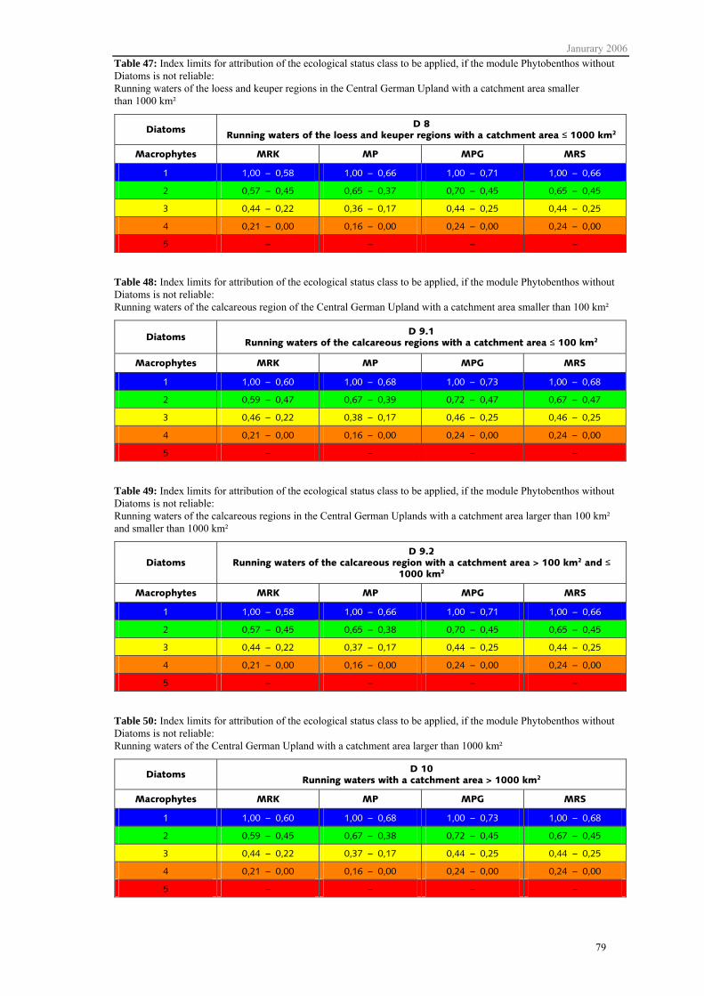
Janurary 2006

79

Table 47: Index limits for attribution of the ecological status class to be applied, if the module Phytobenthos without Diatoms is not reliable: Running waters of the loess and keuper regions in the Central German Upland with a catchment area smaller than 1000 km²

Diatoms D 8 Running waters of the loess and keuper regions with a catchment area ≤ 1000 km2


1 1,00 – 0,58 1,00 – 0,66 1,00 – 0,71 1,00 – 0,66

2 0,57 – 0,45 0,65 – 0,37 0,70 – 0,45 0,65 – 0,45

3 0,44 – 0,22 0,36 – 0,17 0,44 – 0,25 0,44 – 0,25

4 0,21 – 0,00 0,16 – 0,00 0,24 – 0,00 0,24 – 0,00

5 – – – –

Table 48: Index limits for attribution of the ecological status class to be applied, if the module Phytobenthos without Diatoms is not reliable: Running waters of the calcareous region of the Central German Upland with a catchment area smaller than 100 km²

Diatoms D 9.1

Running waters of the calcareous regions with a catchment area ≤ 100 km2


1 1,00 – 0,60 1,00 – 0,68 1,00 – 0,73 1,00 – 0,68

2 0,59 – 0,47 0,67 – 0,39 0,72 – 0,47 0,67 – 0,47

3 0,46 – 0,22 0,38 – 0,17 0,46 – 0,25 0,46 – 0,25

4 0,21 – 0,00 0,16 – 0,00 0,24 – 0,00 0,24 – 0,00

5 – – – –

Table 49: Index limits for attribution of the ecological status class to be applied, if the module Phytobenthos without Diatoms is not reliable: Running waters of the calcareous regions in the Central German Uplands with a catchment area larger than 100 km² and smaller than 1000 km²

Diatoms D 9.2

Running waters of the calcareous region with a catchment area > 100 km2 and ≤ 1000 km2


1 1,00 – 0,58 1,00 – 0,66 1,00 – 0,71 1,00 – 0,66

2 0,57 – 0,45 0,65 – 0,38 0,70 – 0,45 0,65 – 0,45

3 0,44 – 0,22 0,37 – 0,17 0,44 – 0,25 0,44 – 0,25

4 0,21 – 0,00 0,16 – 0,00 0,24 – 0,00 0,24 – 0,00

5 – – – –

Table 50: Index limits for attribution of the ecological status class to be applied, if the module Phytobenthos without Diatoms is not reliable: Running waters of the Central German Upland with a catchment area larger than 1000 km²



1 1,00 – 0,60 1,00 – 0,68 1,00 – 0,73 1,00 – 0,68

2 0,59 – 0,45 0,67 – 0,38 0,72 – 0,45 0,67 – 0,45

3 0,44 – 0,22 0,37 – 0,17 0,44 – 0,25 0,44 – 0,25

4 0,21 – 0,00 0,16 – 0,00 0,24 – 0,00 0,24 – 0,00

5 – – – –

January 2006

80

Assessment with the modules Macrophytes and Phytobenthos without Diatoms to be applied, if the module Diatoms is not reliable

Table 51: Index limits for attribution of the ecological status class to be applied, if the module Diatoms is not reliable: siliceous running waters of the Central German Upland

Phytobenthos MG_sil


1 1,00 – 0,67 1,00 – 0,75 1,00 – 0,80 1,00 – 0,75

2 0,66 – 0,55 0,74 – 0,48 0,79 – 0,55 0,74 – 0,55

3 0,54 – 0,30 0,47 – 0,25 0,54 – 0,33 0,54 – 0,33

4 0,29 – 0,00 0,24 – 0,00 0,32 – 0,00 0,32 – 0,00

5 – – – –

Table 52: Index limits for attribution of the ecological status class to be applied, if the module Diatoms is not reliable: calcareous running waters of the Central German Upland



1 1,00 – 0,67 1,00 – 0,75 1,00 – 0,80 1,00 – 0,75

2 0,66 – 0,55 0,74 – 0,48 0,79 – 0,55 0,74 – 0,55

3 0,54 – 0,30 0,47 – 0,25 0,54 – 0,33 0,54 – 0,33

4 0,29 – 0,00 0,24 – 0,00 0,32 – 0,00 0,32 – 0,00

5 – – – –

Janurary 2006

81

Assessment with the modules Diatoms and Phytobenthos without Diatoms to be applied, if the module Macrophytes is not reliable

Table 53: Index limits for attribution of the ecological status class to be applied, if the module Macrophytes is not reliable: siliceous running waters of the Central German Upland

Phytobenthos MG_sil

Diatoms

D 5 Running waters of

variegated sandstone and bedrock with a catchment area

< 100 km2

D 6 Running waters of volcanic regions


< 100 km2


variegated sandstone and bedrock with a

catchment area > 100 km2 and <

1000 km2

1 1,00 – 0,71 1,00 – 0,68 1,00 – 0,68

2 0,70 – 0,52 0,67 – 0,50 0,67 – 0,50

3 0,51 – 0,32 0,49 – 0,32 0,49 – 0,32

4 0,31 – 0,17 0,31 – 0,17 0,31 – 0,17

5 0,16 – 0,00 0,16 – 0,00 0,16 – 0,00

Table 54: Index limits for attribution of the ecological status class to be applied, if the module Macrophytes is not reliable: calcareous running waters of the Central German Upland


Diatoms


the loess and keuper regions with

a catchment area ≤ 1000 km2

D 9.1 Running waters of

the calcareous regions with a

catchment area ≤ 100 km2

D 9.2 Running waters of

the calcareous regions with a

catchment area > 100 km2 and ≤

1000 km2

D 10 Running waters


> 1000 km2

1 1,00 – 0,66 1,00 – 0,68 1,00 – 0,66 1,00 – 0,68

2 0,65 – 0,50 0,67 – 0,52 0,65 – 0,50 0,67 – 0,50

3 0,49 – 0,32 0,51 – 0,32 0,49 – 0,32 0,49 – 0,32

4 0,31 – 0,17 0,31 – 0,17 0,31 – 0,17 0,31 – 0,17

5 0,16 – 0,00 0,16 – 0,00 0,16 – 0,00 0,16 – 0,00

January 2006

82

Assessment with the module Macrophytes to be applied, if the module Diatoms and the module Phytobenthos are not reliable

Table 55 Index limits for attribution of the ecological status class to be applied, if the module Phytobenthos without Diatoms is not reliable: running waters of the Central German Upland


1 1,00 – 0,59 1,00 – 0,75 1,00 – 0,85 1,00 – 0,75

2 0,58 – 0,50 0,74 – 0,35 0,84 – 0,50 0,74 – 0,51

3 0,49 – 0,20 0,34 – 0,10 0,49 – 0,25 0,50 – 0,25

4 0,19 – 0,00 0,09 – 0,00 0,24 – 0,00 0,24 – 0,00

5 – – – –

Assessment with the module Diatoms to be applied, if the module Macrophytes and the module Phytobenthos without Diatoms are not reliable

Table 56: Index limits for attribution of the ecological status class to be applied, if the module Macrophytes and the module Phytobenthos without Diatoms are not reliable: siliceous running waters of the Central German Upland

Diatoms


the variegated sandstone and bedrock with a catchment area

< 100 km2

D 6 Running waters of volcanic regions


< 100 km2


the variegated sandstone and bedrock with a catchment area > 100 km2 and

< 1000 km2

1 1,00 – 0,67 1,00 – 0,61 1,00 – 0,61

2 0,66 – 0,43 0,60 – 0,40 0,60 – 0,40

3 0,42 – 0,24 0,39 – 0,24 0,39 – 0,24

4 0,23 – 0,08 0,23 – 0,08 0,23 – 0,08

5 0,07 – 0,00 0,07 – 0,00 0,07 – 0,00

Table 57: Index limits for attribution of the ecological status class to be applied, if the module Macrophytes and the module Phytobenthos without Diatoms is not reliable: Calcareous running waters of the Central German Upland

Diatoms


the loess and keuper regions with

a catchment area ≤ 1000 km2

D 9.1 Running waters of calcareous regions with a catchment

area ≤ 100 km2

D 9.2 Running waters of calcareous regions with a catchment area > 100 km2 and ≤ 1000 km2

D 10 Running waters


> 1000 km2

1 1,00 – 0,56 1,00 – 0,61 1,00 – 0,57 1,00 – 0,60

2 0,55 – 0,39 0,60 – 0,43 0,56 – 0,40 0,59 – 0,40

3 0,38 – 0,24 0,42 – 0,24 0,39 – 0,24 0,39 – 0,24

4 0,23 – 0,08 0,23 – 0,08 0,23 – 0,08 0,23 – 0,08

5 0,07 – 0,00 0,07 – 0,00 0,07 – 0,00 0,07 – 0,00

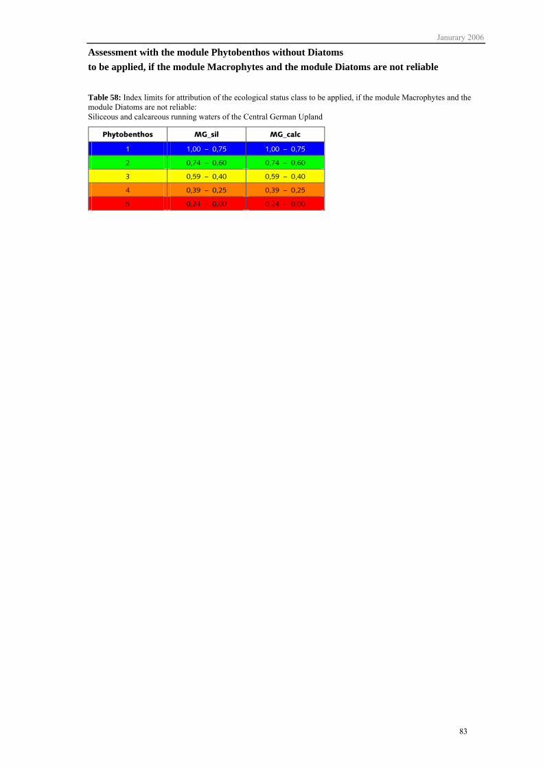
Janurary 2006

83

Assessment with the module Phytobenthos without Diatoms to be applied, if the module Macrophytes and the module Diatoms are not reliable

Table 58: Index limits for attribution of the ecological status class to be applied, if the module Macrophytes and the module Diatoms are not reliable: Siliceous and calcareous running waters of the Central German Upland

Phytobenthos MG_sil MG_calc

1 1,00 – 0,75 1,00 – 0,75

2 0,74 – 0,60 0,74 – 0,60

3 0,59 – 0,40 0,59 – 0,40

4 0,39 – 0,25 0,39 – 0,25

5 0,24 – 0,00 0,24 – 0,00

January 2006

84

4.4.2.4 North German Lowland

Assessment with the modules Macrophytes, Diatoms and Phytobenthos without Diatoms

Table 59: Index limits for attribution of the ecological status class: siliceous or organic running waters of the North German Lowland with a catchment area smaller than 1000 km²

Phytobenthos NT_org/sil

Diatoms D 11 Siliceous running waters with a catchment area ≤ 1000 km2

Macrophytes TR TNk TN TNg

1 1,00 – 0,72 1,00 – 0,68 1,00 – 0,67 1,00 – 0,64

2 0,71 – 0,51 0,67 – 0,51 0,66 – 0,48 0,63 – 0,44

3 0,50 – 0,28 0,50 – 0,30 0,47 – 0,28 0,43 – 0,26

4 0,27 – 0,00 0,29 – 0,00 0,27 – 0,00 0,25 – 0,00

5 – – – –

Table 60: Index limits for attribution of the ecological status class: calcareous running waters of the North German Lowland with a catchment area smaller than 1000 km²

Phytobenthos NT_calc

Diatoms D 12 Calcareous running waters with a catchment area ≤ 1000 km2


1 1,00 – 0,70 1,00 – 0,66 1,00 – 0,65 1,00 – 0,62

2 0,69 – 0,51 0,65 – 0,51 0,64 – 0,48 0,61 – 0,44

3 0,50 – 0,28 0,50 – 0,30 0,47 – 0,28 0,43 – 0,26

4 0,27 – 0,00 0,29 – 0,00 0,27 – 0,00 0,25 – 0,00

5 – – – –

Table 61: Index limits for attribution of the ecological status class: calcareous running waters of the North German Lowland with a catchment area larger than 1000 km²




1 1,00 – 0,74 1,00 – 0,70 1,00 – 0,69 1,00 – 0,66

2 0,73 – 0,55 0,69 – 0,55 0,68 – 0,52 0,65 – 0,48

3 0,54 – 0,32 0,54 – 0,34 0,51 – 0,32 0,47 – 0,30

4 0,31 – 0,00 0,33 – 0,00 0,31 – 0,00 0,29 – 0,00

5 – – – –

Janurary 2006

85

Assessment with the modules Macrophytes and Diatoms to be applied, if the module Phytobenthos without Diatoms is not reliable

Table 62: Index limits for attribution of the ecological status class to be applied, if the module Phytobenthos without Diatoms is not reliable: siliceous or organic running waters of the North German Lowland with a catchment area smaller than 100 km²

Diatoms D 11 Siliceous running waters with a catchment area ≤ 1000 km2


1 1,00 – 0,71 1,00 – 0,65 1,00 – 0,62 1,00 – 0,59

2 0,70 – 0,47 0,64 – 0,47 0,61 – 0,42 0,58 – 0,37

3 0,46 – 0,22 0,46 – 0,25 0,41 – 0,22 0,36 – 0,20

4 0,21 – 0,00 0,24 – 0,00 0,21 – 0,00 0,19 – 0,00

5 – – – –

Table 63: Index limits for attribution of the ecological status class to be applied, if the module Phytobenthos without Diatoms is not reliable: calcareous running waters of the North German Lowland with a catchment area smaller than 1000 km²

Diatoms D 12 Calcareous running waters with a catchment area ≤ 1000 km2


1 1,00 – 0,68 1,00 – 0,62 1,00 – 0,59 1,00 – 0,56

2 0,67 – 0,47 0,61 – 0,47 0,58 – 0,42 0,55 – 0,37

3 0,46 – 0,22 0,46 – 0,25 0,41 – 0,22 0,36 – 0,20

4 0,21 – 0,00 0,24 – 0,00 0,21 – 0,00 0,19 – 0,00

5 – – – –

Table 64: Index limits for attribution of the ecological status class to be applied, if the module Phytobenthos without Diatoms is not reliable: Running waters of the North German Lowland with a catchment area larger than 1000 km²



1 1,00 – 0,74 1,00 – 0,68 1,00 – 0,65 1,00 – 0,62

2 0,73 – 0,53 0,67 – 0,53 0,64 – 0,48 0,61 – 0,43

3 0,52 – 0,28 0,52 – 0,31 0,47 – 0,28 0,42 – 0,26

4 0,27 – 0,00 0,30 – 0,00 0,27 – 0,00 0,25 – 0,00

5 – – – –

January 2006

86

Assessment with the module Macrophytes and the module Phytobenthos without Diatoms

Table 65: Index values for attribution of the ecological status class to be applied, if the module Diatoms is not reliable: siliceous or organic running waters of the North German Lowland



1 1,00 – 0,75 1,00 – 0,69 1,00 – 0,66 1,00 – 0,63

2 0,74 – 0,55 0,68 – 0,55 0,65 – 0,50 0,62 – 0,45

3 0,54 – 0,30 0,54 – 0,33 0,49 – 0,30 0,44 – 0,28

4 0,29 – 0,13 0,32 – 0,13 0,29 – 0,13 0,27 – 0,13

5 - - - -

Table 66: Index limits for attribution of the ecological status class to be applied, if the module Diatoms is not reliable: calcareous running waters of the North German Lowland



1 1,00 – 0,75 1,00 – 0,69 1,00 – 0,66 1,00 – 0,63

2 0,74 – 0,55 0,68 – 0,55 0,65 – 0,50 0,62 – 0,45

3 0,54 – 0,30 0,54 – 0,33 0,49 – 0,30 0,44 – 0,28

4 0,29 – 0,13 0,32 – 0,13 0,29 – 0,13 0,27 – 0,13

5 - - - -

Janurary 2006

87

Assessment with the module Diatoms and Phytobenthos without Diatoms to be applied, if the module Macrophytes is not reliable

Table 67: Index limits for attribution of the ecological status class to be applied, if the module Macrophytes is not reliable: siliceous or organic running waters of the North German Lowland with a catchment area smaller than 100 km²


Diatoms



≤ 1000 km2

1 1,00 – 0,71

2 0,70 – 0,52

3 0,51 – 0,32

4 0,31 – 0,17

5 0,16 – 0,00

Table 68: Index values for attribution of the ecological status class to be applied, if the module Macrophytes is not reliable: calcareous running waters of the North German Lowland


Diatoms


waters with a catchment area ≤

1000 km2

D 13 Running waters


> 1000 km2

1 1,00 – 0,68 1,00 – 0,74

2 0,67 – 0,52 0,73 – 0,58

3 0,51 – 0,32 0,57 – 0,38

4 0,31 – 0,17 0,37 – 0,20

5 0,16 – 0,00 0,19 – 0,00

January 2006

88

Assessment with the module Macrophytes to be applied, if the module Diatoms and the module Phytobenthos without Diatoms is not reliable

Table 69: Index limits for attribution of the ecological status class to be applied, if the module Diatoms and the module Phytobenthos without Diatoms are unreliable: running waters of the North German Lowland


1 1,00 – 0,75 1,00 – 0,63 1,00 – 0,58 1,00 – 0,50

2 0,75 – 0,50 0,62 – 0,50 0,57 – 0,40 0,50 – 0,30

3 0,50 – 0,20 0,50 – 0,25 0,40 – 0,20 0,30 – 0,15

4 0,20 – 0,00 0,25 – 0,00 0,20 – 0,00 0,15 – 0,00

5 – – – –

Assessment with the module Diatoms to be applied, if the module Macrophytes and the module Phytobenthos without Diatoms are unreliable

Table 70: Index limits for the attribution of the ecological status class to be applied, if the module Macrophytes and the module Phytobenthos without Diatoms are unreliable: siliceous or organic and calcareous running waters of the North German Lowland

Diatoms



≤ 1000 km2


waters with a catchment area ≤

1000 km2

D 13 Running waters


> 1000 km2

1 1,00 – 0,67 1,00 – 0,61 1,00 – 0,73

2 0,66 – 0,43 0,60 – 0,43 0,72 – 0,55

3 0,42 – 0,24 0,42 – 0,24 0,54 – 0,36

4 0,23 – 0,08 0,23 – 0,08 0,35 – 0,14

5 0,07 – 0,00 0,07 – 0,00 0,13 – 0,00

Assessment with the module Phytobenthos without Diatoms to be applied, if the modules Macrophytes and Diatoms are not reliable

Table 71: Index limits for attribution of the ecological status class to be applied, if the modules Macrophytes and Diatoms are not reliable: siliceous or organic and calcareous running waters of the North German Lowland

Phytobenthos NT_org/sil NT_calc

1 1,00 – 0,75 1,00 – 0,75

2 0,74 – 0,60 0,74 – 0,60

3 0,59 – 0,40 0,59 – 0,40

4 0,39 – 0,25 0,39 – 0,25

5 0,24 – 0,00 0,24 – 0,00

Janurary 2006

89

4.4.2.5 Combination of the results with additional criteria

After determination of the ecological status by calculating the respective index values, the individual assessment procedures for the modules Macrophytes and Diatoms call for a verification of different metrics indicating different kinds of stress. These additional criteria are also considered for determination of the biocomponent Macrophytes & Phytobenthos. For the different kinds of stress cannot equally well be indicated by all groups of organisms, in the end they are considered for the overall assessment.

If the module „Acidification“ is relevant, the ecological status class is downgraded correspondingly. Due to the particular ecological relevance of this stress factor, downgrading is only carried out in the process of overall assessment after combination of the three sub modules Macrophytes, Diatoms and Phytobenthos without Diatoms to determine the ecological status class Macrophytes & Phytobenthos. This procedure corresponds to the guidelines of ECOSTAT (2003).

(If not noted otherwise) all prerequisites for the application of additional criteria as well as for modifications of the results refer to the overall assessment, i.e. the ecological status class of the entire biocomponent Macrophytes & Phytobenthos!

Macrophyte depopulation

For all ecoregions and for all biocoenotic types of macrophytes the reason for a lack of macrophytes is to be determined. If it can be proven that macrophyte depopulation is the consequence of degradation, for example due to chemical physical parameters, structural modifications (embankments), mowing, clearing or introduction of herbivorous fish or other anthropogenic influences, a “high” or “good” overall assessment must be downgraded to be ecological status class 3.

Acidification

Macrophytes

Type MRS if 100% of the mosses = V and the ecological status class is 1 or 2 downgrade to status class 3 unless the module Acidification Diatoms indicates

a more severe acidification

Diatoms

Types D 5, D 6, D7 Relevance module Acidification downgrade according to Table 20, page 42

January 2006

90

4.5 Expenditure of time

4.5.1 Macrophytes

Duration of macrophyte mapping in the field (compare instruction protocol) amounts to approx. 30 minutes to 1 (maximal 2) hour(s) per sampling site. Time required for travelling to the sampling site can vary considerably and must also be considered. Determination of critical species (e.g. mosses) can require additional time.

Depending on the local conditions and time required to ensure personal safety, mapping can be carried out by one to two people. A detailed mapping procedure during which also the optional fields of the field protocol are filled in maximally takes ten minutes longer than mapping without filling in the optional fields. For an experienced field worker filling in the field report for mapping structural quality according to LAWA (LÄNDER WORKING GROUP WATER 2000) takes 10 to 15 minutes.

4.5.2 Diatoms

Determination of the ecological status of a river section consists of sampling, preparation of the diatom sampling material, determination of species composition and species abundance by counting 400 valves under the light microscope, entering the data regarding the diatom assemblages and calculating the required metrics and the resulting ecological status class. For sampling (planning and travelling excluded) approximately 20 minutes are estimated. The mean processing time of the diatom sample depends on the preparation method and the respective number of samples or the size of the available hot plate. For a preparation by oxidation in salt and sulphuric acid with subsequent preservation of the samples and mounting of permanent samples the estimated time frame is two to three days – up to 50 samples the additional effort required for an increasing number of samples can be neglected. Depending on the density of valves in the sample and the diversity of the assemblages, the microscopic evaluation by an expert amounts to approximately one to three hours. For entering the data into a database on average 20 minutes are estimated. The effort required for evaluating the entered data and carrying out the assessment depends on the availability of a special software.

4.5.3 Phytobenthos without Diatoms, simplified procedure

Sampling (including filling in the field protocol) takes between 30 minutes and 1 h depending on the structural diversity of the sampling site. In addition, the time required for travelling to and finding the sampling site must be considered, which depends on the local conditions. If the samples cannot be evaluated immediately after sampling, they must be preserved in the lab, labelled exactly and stored adequately. For each sampling site these steps take 20 to 30 minutes.

Janurary 2006

91

Depending on the substratum of the sub samples for the simplified procedure on average microscopic analysis should not take longer than three to four hours per sampling site.

If a database is already available, entering the sampling data does not require much time. In such cases calculation of the Assessment Index can be carried out in a fast and convenient fashion. However, the time required for creating and maintaining a database must be kept in mind.

4.5.4 Overall procedure

An overview of the time required is given in Table 72. The time required for travelling to and finding the respective sampling sites is not considered. For preparation of up to 50 diatom samples the processing time required is two to three days. For this reason the preparation is not listed in the table.

Table 72: Overview of the average time required for assessment of the component Macrophytes & Phytobenthos according to the WFD for each sampling site and sampling procedure

Mean expenditure of time

Macrophytes 2,5 h

Diatoms 3 h

Phytobenthos without Diatoms 5 h

Overall 10,5 h

January 2006

92

Janurary 2006

93

Appendix A Characteristics of the biocoenotic macrophyte types

Janurary 2006

95

Siliceous-rhithral running waters of the Central German Upland and the Alps and Alpine Foreland (MRS)

Figure 2: Type MRS: Schwarzbach near Jagdschlösschen (sampling site Nr. 33, Bavaria)

The siliceous rhithral running waters of the Central German Uplands, Alps and Alpine Foreland (MRS, Figure 2) due to their geochemistry have lower values of total hardness and acid capacity. In an almost natural state without anthropogenic influences the mean value does not exceed 1,4 mmol/l. Generally MRS type running waters only have a width of approximately three meters, in rare cases of ten meters. Their water level is low, i.e. they are only 30 cm deep. In their pristine state these running waters are usually surrounded by woods and therefore are (strongly) shaded. According to the scale of the BAVARIAN WATER MANAGEMENT AGENCY (1995) the velocity of flow is almost always IV (rapidly running, current with moderate turbulences) or higher (rapid, torrential). These conditions are reflected in the substratum which is dominated by coarse gravel, stones and boulders. Due to these site characteristics the main growth form of aquatic macrophytes is represented especially by aquatic mosses haptophytes, especially mosses. Vascular hydrophytes are rare (modified according to MEILINGER 2003).

January 2006

96

Janurary 2006

97

Calcareous rhitrhal running waters of the Central German Upland, the Alpine Foreland and the Alps (MRK)

Figure 3: Type MRK: River Würm close to Mühltal (sampling site Nr. 223, Bavaria)

The calcareous rhithral type of running water of the Central German Upland, the Alpine Foreland and the Alps shows similarities to the siliceous type. However, due to their geochemistry MRK types have higher values of total hardness and acid capacity than MRS types. In an almost natural state without anthropogenic influences the mean value exceeds 1,4 mmol/l. Although larger rivers with a width of more than 30 m and a depth of one meter represent this type, high velocities of flow, i.e. class IV (rapidly running, current with moderate turbulences) and higher (rapid, torrential) (BAVARIAN WATER MANAGEMENT AGENCY 1995) are characteristic for rhitral waters. Shading can also reach high values. Large grain sizes are mostly characteristic for the sediment of rhithral waters of the Central German Uplands. In contrast to the MRS type, for the calcareous rhithral type of the Central German Uplands the portion of stones and boulders is somewhat reduced. Mosses make up most of the macrophyte vegetation. Due to the greater flow of water also hydrophytes can be found, especially in eutrophicated waters (modified according to MEILINGER 2003).

January 2006

98

Janurary 2006

99

Potamal running waters of the Central German Upland, the Alpine Foreland and Alps (MP) including subtype MPG (influenced by groundwater)

Figure 4: Type MPG: Inner Rhine River, Niederhausen (sampling site Nr. 881, Baden-Wuerttemberg)

Potamal running waters of the Central German Upland in terms of their habitat conditions for macrophytes are similar to the potamal running waters of the North German Lowland. The waters of type MP(G) often are about 10 meters wide and have a depth of 30 cm. The degree of shading is usually low and the velocity of flow is characterised by class III (slowly running, current visible, water surface almost smooth, BAVARIAN WATER MANAGEMENT AGENCY 1995). Therefore the portion of fine sediments like mud, sand and fine gravel is high. However, coarse substrata like coarse gravel, stones and boulders also make up a considerable portion of the sediment. These suitable conditions for water plants result in a macrophyte vegetation with a high percentage of hydrophytes (modified according to MEILINGER 2003).

The subtype MPG (influenced by groundwater) is noticeably fed by groundwater. It is characteristic of this type that water temperatures are low in summer (“summer cold”) and high in winter (“winter warm”).

January 2006

100

Janurary 2006

101

TR – rhithral running waters of the North German Lowland

Figure 5: Type TR: Outflow of River Schwärze into Lake Schwärzensee (Sampling site Nr .018; Brandenburg)

The rhithral running waters of the North German Lowland (TR, Figure 5) are often only about two to three meters wide and rarely reach a width of more than ten meters. Water flow is low and generally depth does not exceed 30 cm. Almost natural sites of this type are surrounded by woods and therefore are more or less shaded. The velocity of flow is higher higher than for potamal running waters of the North German Lowland (TN), and is characterised by classes III (slowly running, current visible, water surface almost smooth) and class IV (rapidly running, current with moderate turbulences) according to the BAVARIAN WATER MANAGEMENT AGENCY (1995). The current appears rather turbulent. Substrata consist of sand and/or gravel. The running waters of type TR are characterised by a low flow of water which does not allow e.g. for large pondweeds to grow. Due to these particular local conditions sites with little or no anthropogenic influence are generally colonised by mosses or Berula erecta (submerged and emerged), Ranunculus- und Callitriche-species.

January 2006

102

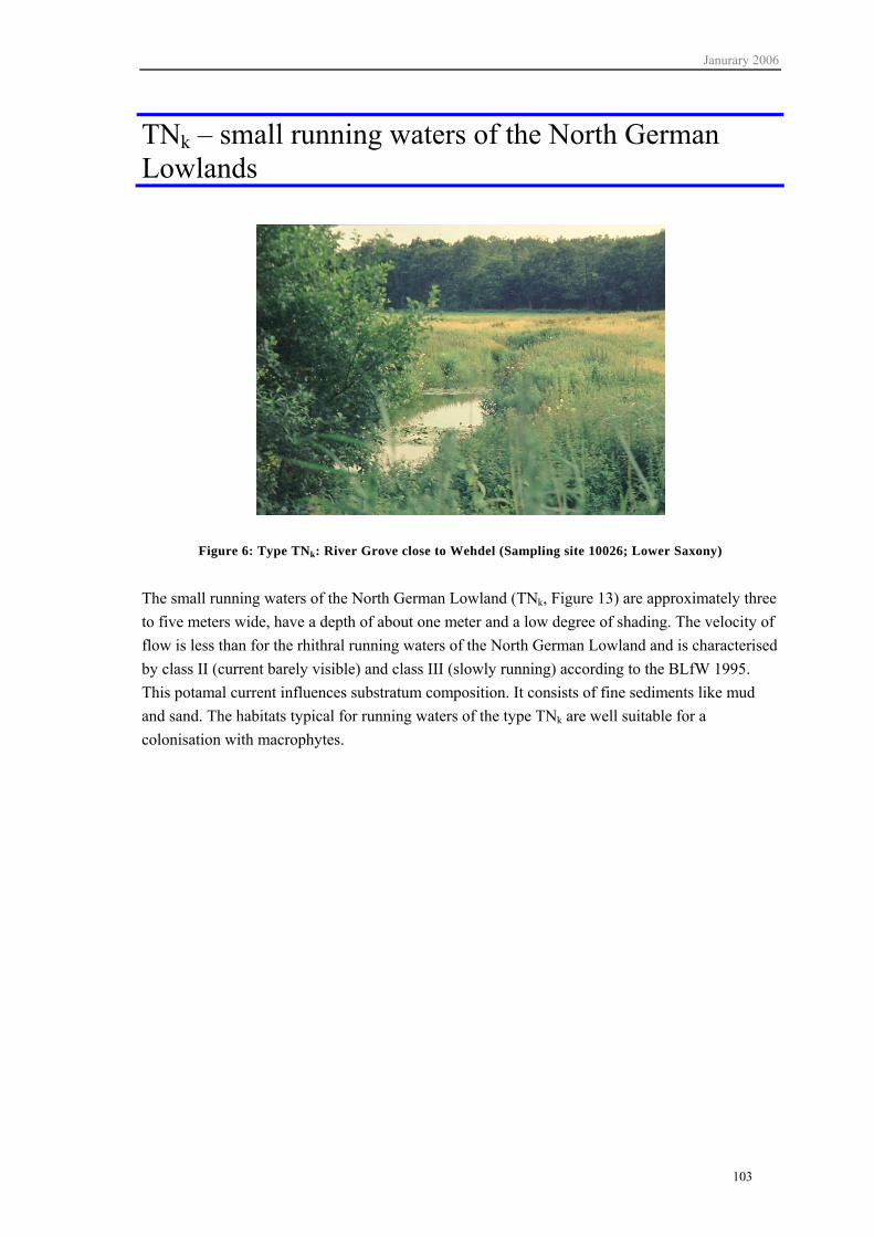
Janurary 2006

103

TNk – small running waters of the North German Lowlands

Figure 6: Type TNk: River Grove close to Wehdel (Sampling site 10026; Lower Saxony)

The small running waters of the North German Lowland (TNk, Figure 13) are approximately three to five meters wide, have a depth of about one meter and a low degree of shading. The velocity of flow is less than for the rhithral running waters of the North German Lowland and is characterised by class II (current barely visible) and class III (slowly running) according to the BLfW 1995. This potamal current influences substratum composition. It consists of fine sediments like mud and sand. The habitats typical for running waters of the type TNk are well suitable for a colonisation with macrophytes.

January 2006

104

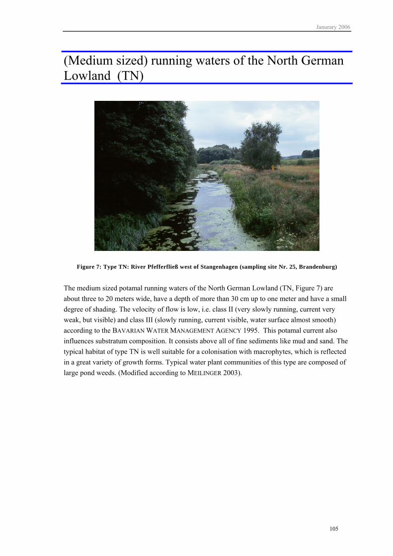
Janurary 2006

105

(Medium sized) running waters of the North German Lowland (TN)

Figure 7: Type TN: River Pfefferfließ west of Stangenhagen (sampling site Nr. 25, Brandenburg)

The medium sized potamal running waters of the North German Lowland (TN, Figure 7) are about three to 20 meters wide, have a depth of more than 30 cm up to one meter and have a small degree of shading. The velocity of flow is low, i.e. class II (very slowly running, current very weak, but visible) and class III (slowly running, current visible, water surface almost smooth) according to the BAVARIAN WATER MANAGEMENT AGENCY 1995. This potamal current also influences substratum composition. It consists above all of fine sediments like mud and sand. The typical habitat of type TN is well suitable for a colonisation with macrophytes, which is reflected in a great variety of growth forms. Typical water plant communities of this type are composed of large pond weeds. (Modified according to MEILINGER 2003).

January 2006

106

Janurary 2006

107

TNg – large running waters of the North German Lowland

Figure 8: Type TNg: River Weser close to Dörverdev (sampling site 10084; Lower Saxony)

The large potamal running waters of the North German Lowland (TNg, Figure 15) have a width of at least 30 meters. In their pristine state they have a wide and shallow profile with frequent formation of furts. Wide spaced changes in the water course, formation of deltas (Figure 8) as well as a high amount of coarse woody debris are characteristic. Due to hydraulic engeneering these running waters today are relatively deep, which does not provide the original basis for colonisation with macrophytes, but limits their occurrence to the border areas. For this reason, in many cases, an assessment with macrophytes is not possible.

January 2006

108

Janurary 2006

109

Appendix B Fixatives for the phytobenthos sampling procedure

acidic Lugol’s solution 20 g potassium iodide (IK)

200 ml distilled water

10 g resublimated iodine (J2)

19 ml glacial acetic acid (96-100% CH3COOH)

Dissolve potassium iodide in a little water, then add iodine and the remaining water. Afterwards add glacial acetic acid. Keep the solution in small brown bottles. It is recommended to fill the bottles well as iodide is oxidised in half empty bottles.

neutralised formaldehyde 500 ml formaldehyde (40%)

500 ml aqua dest.

100 g Hexamethylentetramine

Dilute formaldehyde in aqua dest. and then add hexamethylentetramine. Filter after one week (pH 7,3-7,9).

For preservation of the samples a final concentration of 3-4% should be reached.

January 2006

110

Janurary 2006

111

Appendix C

January 2006

112

Janurary 2006

113

Field protocol for mapping running water macrophytes(Macrophyte- & Phytobenthos-evaluation according to EC-WFD 2005; gray fields are optional)

Name of water body Length of section Mean widthm m

Sampling site Mean depth Water levelI 0-30 cm dry

II 30-100 cm lowLocation of sampling site III >100 cm medium

high

Nearby town/village Editor Can sampling be carried out over the entire width of the running water? yes no

Sampling Site No. Reprot No. Turbidity Bottom visible?no turbidity, clear yesMedium turbidity no

Easting Northing Strong turbidity

Film-/Photo-No.Topo. Map No. Recording date

Velocity of flow according to BLfW (1995)

I not visible almost still, eddyII barely visible current very weak, but visible

III slowly running current visible, water surface smoothIV rapidly running current with moderate turbulenceV rapid turbulently running

VI torrential very turbulent, loud brawl

Shading according to Wörlein (1992)

1 completely sunny sunny from sunrise to sunset2 sunny in full sun most of the time between sunrise and sunset, but always during the

warmest hours of the day3 partly overcast mostly in the sun, but in the shade during the warmest hours of the day4 half shaded in the shade for more than half of the day and always at noon5 completely shaded completely shaded by trees

Plant cover WaterCovering large areas mosaic Colouration Odour

Substratum Embankment/Foreign substrataSubstratum

Percentage Cover Distance near natural% Mud m Enforcement of river bed% Clay/loam (<0,063 mm) m Modific. In transverse dir.% Sand (0,063-2,0 mm) m Embankment% Fine/med. gravel (2,0-6,3/6,3-20mm) m Outlets% Coarse gravel (20-63 mm) m Pipes% Stones (63-200 mm) m Waste/(construction)debris% Boulders (> 200 mm) m% organic/peat m

Bavarian Environment Agency November 2005 Figure 9: Field protocol running water macrophytes (page1)

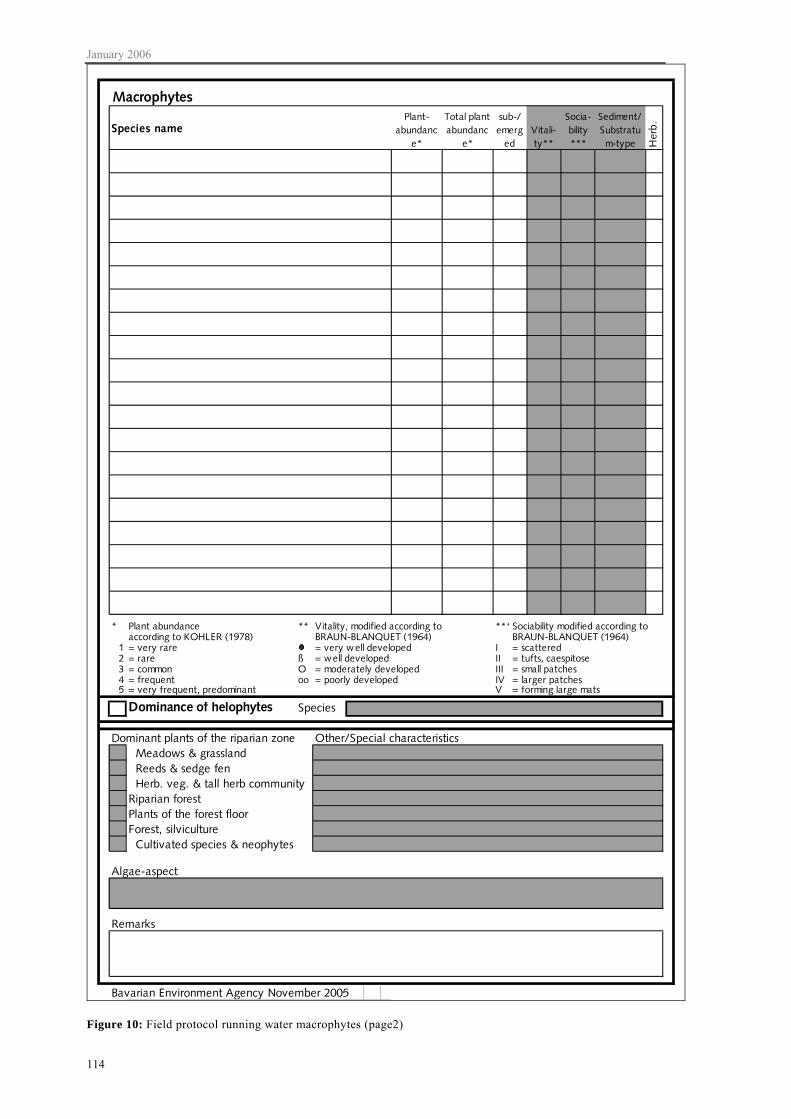
January 2006

114

Macrophytes

Species namePlant-

abundance*

Total plant abundanc

e*

sub-/emerg

edVitali-ty**

Socia-bility***

Sediment/Substratum-type H

erb.

* Plant abundance ** Vitality, modified according to ***Sociability modified according to according to KOHLER (1978) BRAUN-BLANQUET (1964) BRAUN-BLANQUET (1964)

1 = very rare = very well developed I = scattered2 = rare ß = well developed II = tufts, caespitose3 = common O = moderately developed III = small patches4 = frequent oo = poorly developed IV = larger patches5 = very frequent, predominant V = forming large mats

Dominance of helophytes Species

Dominant plants of the riparian zone Other/Special characteristics Meadows & grassland Reeds & sedge fen Herb. veg. & tall herb communityRiparian forestPlants of the forest floorForest, silviculture Cultivated species & neophytes

Algae-aspect

Remarks

Bavarian Environment Agency November 2005

Figure 10: Field protocol running water macrophytes (page2)

Janurary 2006

115

Figure 11: Field protocol for mapping structural quality according to LAWA (2000) (page1)

January 2006

116

Figure 12: Field protocol for mapping structural quality according to LAWA (2000) (page2)

Janurary 2006

117

Field protocol for diatom sampling in running waters(Macrophyte- & Phytobenthos-evaluation according to EC-WFD 2005; gray fields are optional)


Sampling site Mean depth Water levelI 0-30 cm dryII 30-100 cm low

Location of sampling site III >100 cm mediumhigh

Nearby town/village Editor Can sampling be carried out over the entire width of the running water? yes no

Sampling Site No. Report No. Turbidity Bottom visible?no turbidity, clear yesMedium turbidity no


Film-/Photo-No.Topo. Map No. Date

Velocity of flow according to BLfW (1995)

I not visible almost still, eddyII barely visible current very weak, but visible

III slowly running current visible, water surface smoothIV rapidly running current with moderate turbulenceV rapid turbulently running


Shading according to Wörlein (1992)

1 completely sunny sunny from sunrise to sunset2 sunny in full sun most of the time between sunrise and sunset, but always during the

warmest hours of the day3 partly overcast mostly in the sun, but in the shade during the warmest hours of the day4 half shaded in the shade for more than half of the day and always at noon5 completely shaded completely shaded by trees

Substratum diatom sample

Substratum Macrophyte aspect

Percentage% Mud% Clay/loam (<0,063 mm)% Sand (0,063-2,0 mm)% Fine/med. gravel (2,0-6,3/6,3-20 mm) Aspect of remaining phytobenthos% Coarse gravel (20-63 mm)% Stones (63-200 mm)% Boulders (> 200 mm)% organic/peat

Remarks


Figure 13: Field protocol running water diatoms

January 2006

118

Field protocol running water phytobenthos(Macrophyte- & phytobenthos-evaluation according to-WFD 2005; grey fields are optional)


Sampling site mean depth water levelI 0-30 cm dryII 30-100 cm low

Location of sampling site III >100 cm mediumhigh

Nearby town or village Editor Can sampling be carried out over the entire width of the running water? yes no

Sampling site No. Report-No. Turbidity Bottom visible?no turbidity, clear yesmedium turbidity no

Easting Northing strong turbidity

Film-/photo-No.Topo. Map No. Date

Phytobenthos samples

Degree of cover or estimated abundance

1

2

3

4

5

6

7

8

9

10

11

12

13

14

15

16

17

18


Nr. Description of sample Type of substratum

Figure 14: Field protocol running water phytobenthos without diatoms

Janurary 2006

119

Microscopy Protocol PhytobenthosRemarks

NoSamSite

NoSubRep Date of sampling

NoSamSite

Cover slip

PhotoTaxon Abundance 1 2 3 4 5 6 7 8 9 10


Figure 15: Microscopy protocol running water phytobenthos without diatoms

January 2006

120

Field Protocol Macrophytes & Phytobenthos of running waters(Macrophytes- & Phytobenthos evaluation according to EC-WFD 2005; grey fields are optional)

name of water body Length of section Mean widthm m

Sampling site Mean depth Water levelI 0-30 cm dry

II 30-100 cm lowLocation of sampling site III >100 cm medium

high

Nearby town/village Editor Can sampling be carried out over the entire widthof the running water? yes no

Sampling Site-No. Report-No. Turbidity Bottom visibleNo turbidity, clear yesMedium turbidity no


Film-/Photo-No.Top. Map No. Recording date

Velocity of flow according to BLfW (1995) Diatom sample Yes/no

I not visible almost still, eddy Substrate II barely visible current very weak, but visible

III slowly running current visible, water surface smooth

IV rapidly running current with moderate turbulences

V rapidly running turbulently running


Shading according to Wörlein (1992) Macrophyte stands

1 completely sunny sunny from sunrise to sunset covering mosaic2 sunny in full sun most of the time between sunrise andsunset, but large areas

always during the warmest hours of the day

3 partly overcast mostly in the sun, but in shade during the warmest hours of day Water4 half shaded in the shade for more than half of the day and always at noon Colouration5 compl. Shaded completely shaded by trees Odour

Dominance of helophytes Species

Algae aspect

Dominant plants of the riparian zone Remarks Meadows & grassland Reeds & sedge fen Herb veg. & tall herb community Riparian forest Plants of the forest floor Forest, silviculture Cultivated species & neophytes

Substrate Embankments/Foreign substrataSubstrate

Percentage Cover Distance near natural% Mud m Enforcement of river bed % Clay/oam (<0,063 mm) m Modific in transverse dir.% sand (0,063-2,0 mm) m Embankm./Modific. of shore% Fine/med. gravel (2,0-6,3/6,3-20mm) m Outlets% Coarse gravel (20-63 mm) m Pipes% Stones (63-200 mm) m Waste/(construction) debris% Boulders (> 200 mm) m% organic/peat m


Figure 16: Field protocol running water macrophytes and phytobenthos (page 1)

Janurary 2006

121

MacrophytesSpecies name

Plant-abundance

Total plant abundance

sub-/emerge

Vitali-ty**

Sozia-bility**

Sediment/Substrate- H

erb

* Plant abundace according ** Vitalität, verändert nach *** Sociability modified according to to KOHLER (1978) BRAUN-BLANQUET (1964) BRAUN-BLANQUET (1964)

1 = vera rare = very well developed I = scattered2 = rare ß = well developed II = tuts, caespitose3 = common O = moderately developed III = small patches4 = frequent oo = poorly developed IV = larger patches5 = very frequent, predominant V = forming large mats

Phytobenthos samples

1

2

3

4

5

6

7

8

9

10

11

12

13

14

15

16

17

18

19


Type of substratumDegree of cover or estimated abundance

Description of sampleNo

Figure 17: Field protocol running water macrophytes and phytobenthos (page 2)

Instruction Protocol for the ecological Assessment of...

Documents

Transcript of Instruction Protocol for the ecological Assessment of...