Institute on Computational Economics (ICE05)Argonne National Laboratory

July 18 – 22, 2005

Problem-Solving Environments for Optimization: NEOS

Jorge J. More

Mathematics and Computer Science DivisionArgonne National Laboratory

Key Concepts

I Problem-solving environments

I NEOS (Network-Enabled Optimization System)

I Cyberinfrastructure

A problem-solving environment consists of the data, modeling,algorithms, software, hardware, visualization, and communicationtools for solving a class of computational science problems

Optimization problems: AMPL, GAMS, MATLAB, NEOS, . . .

Cyberinfrastructure

Cyberinfrastructure refers to infrastructure based on distributedcomputer, information, and communication technology Thecyberinfrastructure layer is the (distributed) data, modeling,algorithms, software, hardware, and communication tools forsolving scientific and engineering problems.

Blue Ribbon Advisory Panel (Atkins report), February 2003

NSF Workshops

I Cyberinfrastructure and the Social Sciences (SBE-CISE)

I Cyberinfrastructure and Operations Research (CISE-ENG)

Introduction: The Classical Model

Fortran C Matlab AMPL

Solving Optimization Problems: The NEOS Model

A collaborative research project that represents the efforts of theoptimization community by providing access to 50+ solvers fromboth academic and commercial researchers.

OptimizationProblem

NEOSServer

Web browser(HTTP)

Email(SMTP)

NST(Sockets)

Kestrel(Corba)

AdministrationTools

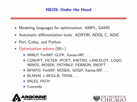
NEOS: Under the Hood

I Modeling languages for optimization: AMPL, GAMS

I Automatic differentiation tools: ADIFOR, ADOL-C, ADIC

I Perl, Corba, and Python

I Optimization solvers (50+)

� MINLP, FortMP, GLPK, Xpress-MP, . . .

� CONOPT, FILTER, IPOPT, KNITRO, LANCELOT, LOQO,MINOS, MOSEK, PATHNLP, PENNON, SNOPT

� BPMPD, FortMP, MOSEK, OOQP, Xpress-MP, . . .

� BLMVM, L-BFGS-B, TRON, . . .

� MILES, PATH

� Concorde

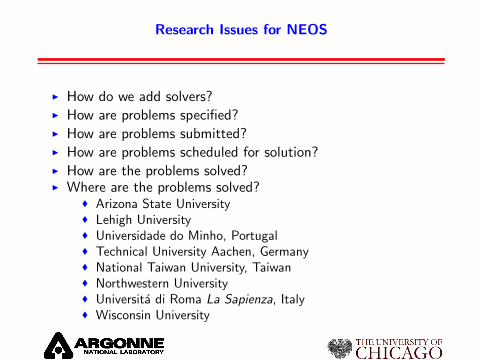
Research Issues for NEOS

I How do we add solvers?I How are problems specified?I How are problems submitted?I How are problems scheduled for solution?I How are the problems solved?I Where are the problems solved?

� Arizona State University� Lehigh University� Universidade do Minho, Portugal� Technical University Aachen, Germany� National Taiwan University, Taiwan� Northwestern University� Universita di Roma La Sapienza, Italy� Wisconsin University

NEOS Submissions: 2000 – 2004

0300060009000

1200015000180002100024000

2000 2001 2002 2003 2004

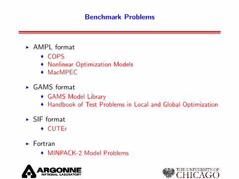
Benchmark Problems

I AMPL format� COPS� Nonlinear Optimization Models� MacMPEC

I GAMS format� GAMS Model Library� Handbook of Test Problems in Local and Global Optimization

I SIF format� CUTEr

I Fortran� MINPACK-2 Model Problems

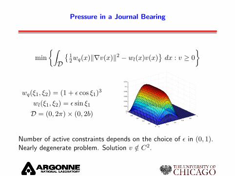
Pressure in a Journal Bearing

min{∫D

{12wq(x)‖∇v(x)‖2 − wl(x)v(x)

}dx : v ≥ 0

}

wq(ξ1, ξ2) = (1 + ε cos ξ1)3

wl(ξ1, ξ2) = ε sin ξ1

D = (0, 2π)× (0, 2b)

00.2

0.40.6

0.81

0

0.2

0.4

0.6

0.8

10

0.02

0.04

0.06

0.08

0.1

0.12

Number of active constraints depends on the choice of ε in (0, 1).Nearly degenerate problem. Solution v /∈ C2.

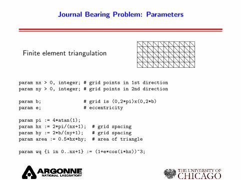
Journal Bearing Problem: Parameters

Finite element triangulation

param nx > 0, integer; # grid points in 1st direction

param ny > 0, integer; # grid points in 2nd direction

param b; # grid is (0,2*pi)x(0,2*b)

param e; # eccentricity

param pi := 4*atan(1);

param hx := 2*pi/(nx+1); # grid spacing

param hy := 2*b/(ny+1); # grid spacing

param area := 0.5*hx*hy; # area of triangle

param wq {i in 0..nx+1} := (1+e*cos(i*hx))^3;

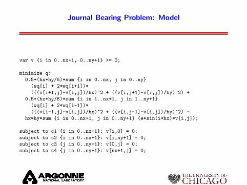
Journal Bearing Problem: Model

var v {i in 0..nx+1, 0..ny+1} >= 0;

minimize q:

0.5*(hx*hy/6)*sum {i in 0..nx, j in 0..ny}

(wq[i] + 2*wq[i+1])*

(((v[i+1,j]-v[i,j])/hx)^2 + ((v[i,j+1]-v[i,j])/hy)^2) +

0.5*(hx*hy/6)*sum {i in 1..nx+1, j in 1..ny+1}

(wq[i] + 2*wq[i-1])*

(((v[i-1,j]-v[i,j])/hx)^2 + ((v[i,j-1]-v[i,j])/hy)^2) -

hx*hy*sum {i in 0..nx+1, j in 0..ny+1} (e*sin(i*hx)*v[i,j]);

subject to c1 {i in 0..nx+1}: v[i,0] = 0;

subject to c2 {i in 0..nx+1}: v[i,ny+1] = 0;

subject to c3 {j in 0..ny+1}: v[0,j] = 0;

subject to c4 {j in 0..ny+1}: v[nx+1,j] = 0;

Journal Bearing Problem: Data

# Set the design parameters

param b := 10;

param e := 0.1;

# Set parameter choices

let nx := 50;

let ny := 50;

# Set the starting point.

let {i in 0..nx+1,j in 0..ny+1} v[i,j]:= max(sin(i*hx),0);

Journal Bearing Problem: Commands

option show_stats 1;

option solver "knitro";

option solver "snopt";

option solver "loqo";

option solver "ipopt";

model;

include bearing.mod;

data;

include bearing.dat;

solve;

printf {i in 0..nx+1,j in 0..ny+1}: "%21.15e\n", v[i,j] > cops.dat;

printf "%10d\n %10d\n", nx, ny >> cops.dat;

NEOS Solver: IPOPT

I Formulation

min {f(x) : xl ≤ x ≤ xu, c(x) = 0}

I Interfaces: AMPLI Second-order information options:

� Differences� Limited memory� Hessian-vector products

I Direct solvers: MA27, MA57

I Documentation

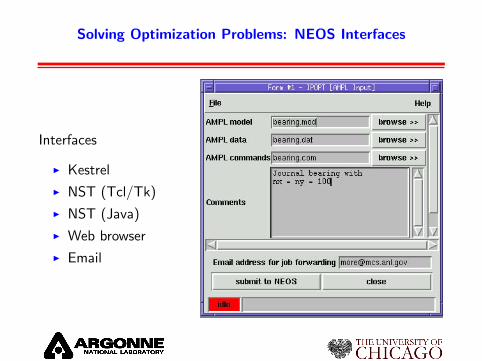
Solving Optimization Problems: NEOS Interfaces

Interfaces

I Kestrel

I NST (Tcl/Tk)

I NST (Java)

I Web browser

I Email

Isomerization of α-pinene

Determine the reaction coefficients in the thermal isomerization ofα-pinene from measurements z1, . . . z8 by minimizing

8∑j=1

‖y(τj ; θ)− zj‖2

y′1 = −(θ1 + θ2)y1

y′2 = θ1y1

y′3 = θ2y1 − (θ3 + θ4)y3 + θ5y5

y′4 = θ3y3

y′5 = θ4y3 − θ5y5

α-pinene Problem: Collocation Formulation

var v {1..nh,1..ne};

var w {1..nh,1..nc,1..ne};

var uc {i in 1..nh, j in 1..nc, s in 1..ne} =

v[i,s] + h*sum {k in 1..nc} w[i,k,s]*(rho[j]^k/fact[k]);

var Duc {i in 1..nh, j in 1..nc, s in 1..ne} =

sum {k in 1..nc} w[i,k,s]*(rho[j]^(k-1)/fact[k-1]);

minimize l2error:

sum {j in 1..nm} (sum {s in 1..ne}(v[itau[j],s] + (

sum {k in 1..nc} w[itau[j],k,s]*

(tau[j]-t[itau[j]])^k/(fact[k]*h^(k-1))) - z[j,s])^2) ;

subject to theta_bounds {i in 1..np}: theta[i] >= 0.0;

subject to ode_bc {s in 1..ne}: v[1,s] = bc[s];

α-pinene Problem: Collocation Conditions

subject to continuity {i in 1..nh-1, s in 1..ne}:

v[i,s] + h*sum {j in 1..nc} (w[i,j,s]/fact[j]) = v[i+1,s];

subject to de1 {i in 1..nh, j in 1..nc}:

Duc[i,j,1] = - (theta[1]+theta[2])*uc[i,j,1];

subject to de2 {i in 1..nh, j in 1..nc}:

Duc[i,j,2] = theta[1]*uc[i,j,1];

subject to de3 {i in 1..nh, j in 1..nc}:

Duc[i,j,3] = theta[2]*uc[i,j,1] - (theta[3]+theta[4])*uc[i,j,3] +

theta[5]*uc[i,j,5];

subject to de4 {i in 1..nh, j in 1..nc}:

Duc[i,j,4] = theta[3]*uc[i,j,3];

subject to de5 {i in 1..nh, j in 1..nc}:

Duc[i,j,5] = theta[4]*uc[i,j,3] - theta[5]*uc[i,j,5];

Flow in a Channel Problem

Analyze the flow of a fluid during injection into a long verticalchannel, assuming that the flow is modeled by the boundary valueproblem below, where u is the potential function and R is theReynolds number.

u′′′′ = R (u′u′′ − uu′′′)u(0) = 0, u(1) = 1u′(0) = u′(1) = 0

Flow in a Channel Problem: Collocation Formulation

var v {i in 1..nh,j in 1..nd};

var w {1..nh,1..nc};

var uc {i in 1..nh, j in 1..nc, s in 1..nd} =

v[i,s] + h*sum {k in 1..nc} w[i,k]*(rho[j]^k/fact[k]);

var Duc {i in 1..nh, j in 1..nc, s in 1..nd} =

sum {k in s..nd} v[i,k]*((rho[j]*h)^(k-s)/fact[k-s]) + h^(nd-s+1)*

sum {k in 1..nc} w[i,k]*(rho[j]^(k+nd-s)/fact[k+nd-s]);

minimize constant_objective: 1.0;

subject to bc_1: v[1,1] = bc[1,1];

subject to bc_2: v[1,2] = bc[2,1];

subject to bc_3:

sum {k in 1..nd} v[nh,k]*(h^(k-1)/fact[k-1]) + h^nd*

sum {k in 1..nc} w[nh,k]/fact[k+nd-1] = bc[1,2];

subject to bc_4:

sum {k in 2..nd} v[nh,k]*(h^(k-2)/fact[k-2]) + h^(nd-1)*

sum {k in 1..nc} w[nh,k]/fact[k+nd-2] = bc[2,2];

Flow in a Channel Problem: Commands

option show_stats 1;

option solver "knitro";

option solver "snopt";

option solver "loqo";

option solver "ipopt";

model;

include channel.mod;

data;

include channel.dat;

let R := 0; solve;

printf {i in 1..nh}: "%12.8e \n", v[i,2] > cops.dat;

let R := 100; solve;

printf {i in 1..nh}: "%12.8e \n", v[i,2] > cops2.dat;

let R := 10000; solve;

printf {i in 1..nh}: "%12.8e \n", v[i,2] > cops4.dat;

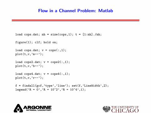
Flow in a Channel Problem: Matlab

load cops.dat; nh = size(cops,1); t = [1:nh]./nh;

figure(1); clf; hold on;

load cops.dat; v = cops(:,1);

plot(t,v,’m--’);

load cops2.dat; v = cops2(:,1);

plot(t,v,’b--’);

load cops4.dat; v = cops4(:,1);

plot(t,v,’r--’);

f = findall(gcf,’type’,’line’); set(f,’LineWidth’,2);

legend(’R = 0’,’R = 10^2’,’R = 10^4’,1);