Institut fur Informatik der Technischen Universit at Munc ...
114
Institut f¨ ur Informatik der Technischen Universit¨ at M¨ unchen Lehrstuhl f¨ ur Informatik XVIII Compact Bidding Languages and Supplier Selection for Markets with Economies of Scale and Scope Stefan Schneider Vollst¨andiger Abdruck der von der Fakult¨at f¨ ur Informatik der Technischen Universit¨ at M¨ unchen zur Erlangung des akademischen Grades eines Doktors der Naturwissenschaften (Dr. rer. nat.) genehmigten Dissertation. Vorsitzender: Univ.-Prof. Dr. Helmut Seidl Pr¨ ufer der Dissertation: 1. Univ.-Prof. Dr. Martin Bichler 2. Univ.-Prof. Gudrun J. Klinker, Ph.D. Die Dissertation wurde am 07.03.2011 bei der Technischen Universit¨at M¨ unchen eingereicht und durch die Fakult¨at f¨ ur Informatik am 30.07.2011 angenommen.
Transcript of Institut fur Informatik der Technischen Universit at Munc ...

Institut fur Informatik
der Technischen Universitat Munchen
Lehrstuhl fur Informatik XVIII
Compact Bidding Languages andSupplier Selection for Markets
with Economies of Scale and Scope
Stefan Schneider
Vollstandiger Abdruck der von der Fakultat fur Informatik der TechnischenUniversitat Munchen zur Erlangung des akademischen Grades eines
Doktors der Naturwissenschaften (Dr. rer. nat.)
genehmigten Dissertation.
Vorsitzender: Univ.-Prof. Dr. Helmut SeidlPrufer der Dissertation:
1. Univ.-Prof. Dr. Martin Bichler2. Univ.-Prof. Gudrun J. Klinker, Ph.D.
Die Dissertation wurde am 07.03.2011 bei der Technischen UniversitatMunchen eingereicht und durch die Fakultat fur Informatik am 30.07.2011angenommen.


Abstract
Preference elicitation is a fundamental problem in single-unit combinatorialauctions, but it becomes prohibitive even for small instances of multi-unitcombinatorial auctions. The bidders cannot express their preferences exactlyas this would take a huge number of bids, typically leading to inefficient allo-cations.
Hence, markets with economies of scale and scope require more compact andyet expressive bidding languages. In this thesis, we propose an expressive bid-ding language allowing bidders to describe the characteristics of their cost func-tions. Bidders in these auctions can specify various discounts and markups,and specify pricing rules as logical functions. Finding the optimal allocationgiven these pricing rules is a strongly NP-hard optimization problem and wepropose a mixed integer program to solve it.
Based on field data, we introduce a multi-item cost function and provide ex-tensive computational experiments to explore the computational burden andthe impact of different language features on the computational effort and totalspend of the auctioneer. In addition, we explore characteristics of the knowl-edge representation of the bidding language.
i

ii
Zusammenfassung
Kombinatorische Auktionen bieten die Moglichkeit Synergieeffekte zu nutzen,indem sie mehrere Guter in einer Auktion zusammenfassen. In einer kombi-natorischen Auktion mit einer nicht trivialen Anzahl von Gutern ist allerdingsbereits das Abfragen der relevanten Wertigkeiten problematisch, da die Bieternicht so viele Einzelgebote abgeben konnen wie notig waren, um die effizienteAllokation sicher zu bestimmen. Dieses Problem verscharft sich weiter, wennpro Gut nicht nur eine Einheit versteigert wird, sondern auch Mengenrabatteberucksichtigt werden sollen.
Daher benotigen derartige Markte kompaktere, und dadurch beherrschbare,aber dennoch erschopfende Bietsprachen. In der vorliegenden Arbeit schla-gen wir eine derartige Sprache vor, welche es den Bietern auf vielfaltigeWeise erlaubt ihre Kostencharakteristika in kompakter und intuitiver Formauszudrucken. Dazu konnen sie verschiedenartige Preismodifikatoren verwen-den, welche ihrerseits von flexiblen und logisch kombinierbaren Bedingungenabhangen. Diese Bedingungen konnen sich dabei sowohl auf die gekaufteMenge als auch den erzielten Umsatz beziehen. Das Bestimmen der opti-malen Allokation aus diesen komplexen Preisstrukturen ist erwiesenermaßenNP vollstandig, und von daher in der Berechnung potentiell sehr aufwandig.Wir schlagen daher ein gemischt-ganzzahliges Optimierungsproblem vor, mitdessen Hilfe diese berechnet werden kann.
Abschließend evaluieren wir unseren Ansatz mit Hilfe eines selbstentwickeltenKostenmodells, dessen Charakteristika auf Echtdaten beruhen, welche wir inFeldversuchen sammeln konnten. Als Hauptergebnis sondieren wir, welcheProblemgroßen in akzeptabler Zeit losbar sind. Wir untersuchen dabei denEinfluss verschiedener Elemente der Bietsprache auf Berechnungsaufwand undEinsparungsmoglichkeiten gegenuber einfacheren Ansatzen.
iii

iv
Acknowledgments
Zuerallerst will ich mich bei Martin Bichler fur die Gelegenheit bedanken, einsolch interessantes und spannendes Forschungsprojekt ubernehmen zu durfen.Die freizugig und gestaltende Arbeit daran hat mir viel Spass bereitet und ichhabe vieles dabei gelernt.
A special thanks goes to Kemal Guler and Mehmet Sayal for a very inspiringcollaboration and the great time in California.
Bei meine Kollgen Georg Ziegler, Pasha Shabalin, Tobias Scheffel, Jurgen Wolf,Alexander Pikovsky, Christian Markl, Oliver Huhn und Christian Hass mochteich mich fur die Diskussionen und wertvolle Anregungen bedanken.
Ich mochte Felix Schmid dafur danken sein Zimmer belagern zu durfen undMaria Schmid fur Ihre treibende Geduld.
v

vi
Contents
Abstract . . . . . . . . . . . . . . . . . . . . . . . . . . . . . . . . . . i
Zusammenfassung . . . . . . . . . . . . . . . . . . . . . . . . . . . . . iii
Acknowledgements . . . . . . . . . . . . . . . . . . . . . . . . . . . . v
List of Figures xi
List of Tables xv
1 Introduction 1
1.1 Motivation . . . . . . . . . . . . . . . . . . . . . . . . . . . . . . 1
1.2 Contributions . . . . . . . . . . . . . . . . . . . . . . . . . . . . 3
1.3 Structure of the Thesis . . . . . . . . . . . . . . . . . . . . . . . 4
2 Combinatorial Auctions and their Applicability to Multi-unitSettings 7
2.1 Characterizations of Multi-item and Multi-unit Auctions . . . . 7
2.2 Iterative Combinatorial Auctions . . . . . . . . . . . . . . . . . 8
2.2.1 Bidding Languages . . . . . . . . . . . . . . . . . . . . . 8
2.2.2 Winner Determination . . . . . . . . . . . . . . . . . . . 10
2.2.3 Non-Linear Personalized Price Auctions . . . . . . . . . 13
2.2.4 Ascending Vickrey Auctions . . . . . . . . . . . . . . . . 14
2.2.5 Linear Price Auctions . . . . . . . . . . . . . . . . . . . 15
vii
2.2.6 Problems . . . . . . . . . . . . . . . . . . . . . . . . . . 16
2.2.7 Evaluation . . . . . . . . . . . . . . . . . . . . . . . . . . 17
2.2.8 Results . . . . . . . . . . . . . . . . . . . . . . . . . . . . 22
2.2.9 Applicability to Procurement Auctions . . . . . . . . . . 35
2.3 Volume Discount Auctions . . . . . . . . . . . . . . . . . . . . . 36
2.3.1 Bidding Languages . . . . . . . . . . . . . . . . . . . . . 36
2.3.2 Winner Determination . . . . . . . . . . . . . . . . . . . 36
2.3.3 Open Issues . . . . . . . . . . . . . . . . . . . . . . . . . 37
3 The LESS Bidding Langue 39
3.1 Bidding Language . . . . . . . . . . . . . . . . . . . . . . . . . . 39
3.1.1 Description Length of Bidding Languages . . . . . . . . . 39
3.1.2 The LESS Bidding Language . . . . . . . . . . . . . . . . 42
4 The Supplier and Quantity Selection 45
4.1 The Supplier Quantity Selection Problem Formulation . . . . . 45
4.2 Scenario Analysis . . . . . . . . . . . . . . . . . . . . . . . . . . 49
4.2.1 Price Feedback in LESS . . . . . . . . . . . . . . . . . . 51
5 Experimental Setup 53
5.1 Value Model ”Cost of Production“ . . . . . . . . . . . . . . . . 53
5.1.1 Composition of Cost . . . . . . . . . . . . . . . . . . . . 54
5.1.2 Parametrizable Cost Function . . . . . . . . . . . . . . . 58
5.2 Bid Generation . . . . . . . . . . . . . . . . . . . . . . . . . . . 64
5.2.1 Fixed Interval Bidding . . . . . . . . . . . . . . . . . . . 65
5.2.2 Fixed Approximation Error Bidding . . . . . . . . . . . . 67
viii

6 Experimental Results 71
6.1 Cost of Flexibility . . . . . . . . . . . . . . . . . . . . . . . . . . 71
6.2 Value Model Cost of Production . . . . . . . . . . . . . . . . . . 75
6.2.1 Single Item Instances . . . . . . . . . . . . . . . . . . . . 75
6.2.2 Single Item Instances with Lump Sum Discounts andMarkups . . . . . . . . . . . . . . . . . . . . . . . . . . . 80
6.2.3 Multi Item Instances - Realistic Problems . . . . . . . . 81
7 Conclusion and Outlook 87
7.1 Conclusion . . . . . . . . . . . . . . . . . . . . . . . . . . . . . . 87
7.2 Outlook . . . . . . . . . . . . . . . . . . . . . . . . . . . . . . . 89
ix

x

List of Figures
2.1 Efficiency and revenue of iterative combinatorial auctions forthe Transportation value model . . . . . . . . . . . . . . . . . . 25
2.2 Efficiency and revenue of iterative combinatorial auctions forthe Real Estate 3x3 value model . . . . . . . . . . . . . . . . . . 26
2.3 Efficiency and revenue of iterative combinatorial auctions forthe Pairwise Synergy value model . . . . . . . . . . . . . . . . . 27
2.4 Rounds needed by iterative combinatorial auctions . . . . . . . 32
2.5 Impact of BSC on prices for straightforward bidding with theReal Estate value model . . . . . . . . . . . . . . . . . . . . . . 33
5.1 Total, average and marginal costs dependent on the number ofunits purchased if only fixed costs of 1000 $ are present . . . . . 55
5.2 Total, average and marginal costs dependent on the number ofunits purchased if only stepwise fixed costs of 200 $ are present . 55
5.3 Total, average and marginal costs dependent on the number ofunits purchased if only variable costs of 1 $ are present . . . . . 56
5.4 Total, average and marginal costs dependent on the number ofunits purchased if fixed costs of 1000 $ and superlinear variablecosts are present . . . . . . . . . . . . . . . . . . . . . . . . . . 57
5.5 Total, average and marginal costs dependent on the number ofunits purchased if stepwise fixed costs of 200 $ and superlinearvariable costs are present . . . . . . . . . . . . . . . . . . . . . . 57
5.6 Cost function base case (not randomized) . . . . . . . . . . . . . 60
xi

5.7 Random instaces of the cost function for seeds 2,3 and 9 . . . . 62
5.8 Random instances of the cost function for seeds 2,3 and 9 anddifferent supplier realizations in dotted lines . . . . . . . . . . . 64
5.9 Comparison of fixed interval bidding with 5 intervals . . . . . . 66
5.10 Comparison of fixed interval bidding with 5 intervals and step-wise fixed costs . . . . . . . . . . . . . . . . . . . . . . . . . . . 67
5.11 Comparison of fixed approximation error bidding with a maxi-mum error of 25% . . . . . . . . . . . . . . . . . . . . . . . . . 68
5.12 Comparison of fixed approximation error bidding with a maxi-mum error of 25% without fixed costs . . . . . . . . . . . . . . . 69
6.1 Description length comparison of incremental vs. total quantitybids in LESS for 32 supplier instances of the base case . . . . . . 76
6.2 Comparison of number of price intervals for different incremen-tal and total quantity bidding policies for 30 single item CoPinstances . . . . . . . . . . . . . . . . . . . . . . . . . . . . . . . 76
6.3 Comparison of computation time for different incremental andtotal quantity bidding policies for 30 single item CoP instanceswith 2 suppliers . . . . . . . . . . . . . . . . . . . . . . . . . . . 77
6.4 Comparison of computation time for different incremental andtotal quantity bidding policies for 30 single item CoP instanceswith 8 suppliers . . . . . . . . . . . . . . . . . . . . . . . . . . . 78
6.5 Comparison of computation time for different incremental andtotal quantity bidding policies for 30 single item CoP instanceswith 64 suppliers . . . . . . . . . . . . . . . . . . . . . . . . . . 78
6.6 Comparison of spend relative to an split award auction for diffe-rent incremental and total quantity bidding policies for 30 singleitem CoP instances with 2 suppliers . . . . . . . . . . . . . . . . 79
6.7 Comparison of spend relative to an split award auction for diffe-rent incremental and total quantity bidding policies for 30 singleitem CoP instances with 64 suppliers . . . . . . . . . . . . . . . 80
6.8 Comparison of computation time for different incremental andtotal quantity bidding policies for 30 single item CoP instanceswith 64 suppliers . . . . . . . . . . . . . . . . . . . . . . . . . . 81
xii

6.9 Comparison of spend relative to a split award auction for diffe-rent incremental and total quantity bidding policies using lumpsum discounts and markups for 30 single item CoP instances . . 81
xiii

xiv

List of Tables
2.1 Performance of iterative combinatorial auctions with differingBidding Agents for the Real Estate value model . . . . . . . . . 22
2.2 Performance of iterative combinatorial auctions with differingBidding Agents for the Pairwise Synergy value model . . . . . . 23
2.3 Performance of iterative combinatorial auctions with differingBidding Agents for the Transportation value model . . . . . . . 24
2.4 Number of instances of the threshold problem in iterative com-binatorial auctions, where small bidders actually won . . . . . . 30
2.5 Comparison of ICAs with differing competition levels . . . . . . 32
2.6 Revenue in % to the VCG outcome, in the Real Estate valuemodel with BSC fulfilled . . . . . . . . . . . . . . . . . . . . . . 33
2.7 Revenue in % to the VCG outcome, in the Real Estate valuemodel with BSC not fulfilled . . . . . . . . . . . . . . . . . . . . 33
4.1 List of Variables in SQS . . . . . . . . . . . . . . . . . . . . . 47
4.2 List of Parameters in SQS . . . . . . . . . . . . . . . . . . . . . 47
4.3 List of Sets in SQS . . . . . . . . . . . . . . . . . . . . . . . . . 48
5.1 Single item cost function parameters . . . . . . . . . . . . . . . 58
5.2 Multi item cost function parameters . . . . . . . . . . . . . . . . 60
5.3 Parameters of the cost funtion in the proposed base case . . . . 61
5.4 Parameters of the cost funtion in the base (singe item) case . . . 63
xv
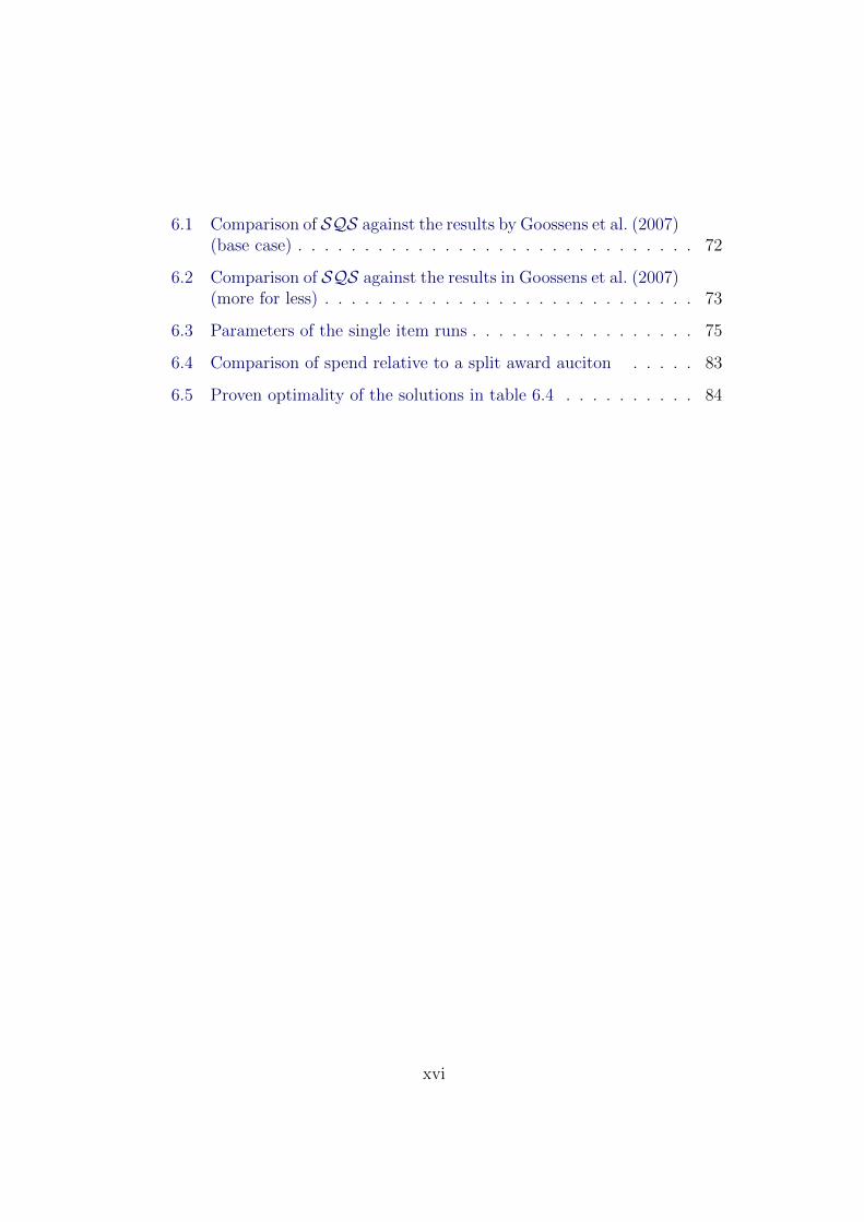
6.1 Comparison of SQS against the results by Goossens et al. (2007)(base case) . . . . . . . . . . . . . . . . . . . . . . . . . . . . . . 72
6.2 Comparison of SQS against the results in Goossens et al. (2007)(more for less) . . . . . . . . . . . . . . . . . . . . . . . . . . . . 73
6.3 Parameters of the single item runs . . . . . . . . . . . . . . . . . 75
6.4 Comparison of spend relative to a split award auciton . . . . . 83
6.5 Proven optimality of the solutions in table 6.4 . . . . . . . . . . 84
xvi

Chapter 1
Introduction
Procurement is one of the key activities in the supply chain and occupies a veryimportant role in the overall performance of a company. With margins dwin-dling, due to increased competition in nearly all industries, it becomes evenmore indispensable to firms to minimize their procurement cost by procuringat the best prices.
Economies of scale and scope describe key characteristics of a supplier’s pro-duction function that influence the prices on procurement markets. Whereaseconomies of scale primarily refer to efficiencies associated with supply-sidechanges, such as increasing or decreasing the scale of production of a singleproduct type, economies of scope refer to efficiencies associated with demand-side changes, such as increasing or decreasing the scope of marketing anddistribution, of different types of products.
Auctions as an advanced mechanism for trading have successfully been usedand eased negotiation in many environments. One of their main features is theability to find prices that reflect the market situation closely by coordinatingthe competition.
1.1 Motivation
Using auctions in procurement is therefore a logical step and simple split-awardauctions are regularly used in practice for multi-item, multi-unit negotiations.There the best bidder gets a predefined larger share of the volume for a par-ticular good and the second best bidder gets the remaining share. This is
1
CHAPTER 1. INTRODUCTION
done to on the one hand assure supply if one supplier is unable to fulfill hiscontract and on the other hand a minimal supplier pool in the long run. Withsignificant economies of scale, suppliers face a strategic problem in these auc-tions. Since there is uncertainty about which quantity they will get awarded,they might speculate and bid less aggressively based on the unit cost for thesmaller, more expensive, share. In other words, simple split award auctions donot allow suppliers to adequately express economies of scale.
In the recent years, driven by the new possibilities of the Internet, a growingliterature is devoted to the design of optimization-based markets (aka. smartmarkets) (Gallien and Wein 2005), and in particular to combinatorial auctions,where bidders are allowed to submit bids on packages of discrete items (Cram-ton et al. 2006). The promise of these mechanisms is that by allowing marketparticipants to reveal more comprehensive information about cost structuresor utility functions, this can drastically increase allocative efficiency and leadto higher economic welfare. Unfortunately, the matching of complex preferenceprofiles typically leads to hard optimization problems. The literature in thisfield is typically focused on multi-item but single-unit negotiations and respec-tive auction formats do not easily extend to multi-unit markets with economiesof scale. While preference elicitation is already a fundamental problem for bid-ders in single-unit combinatorial auctions, it becomes prohibitive in multi-unitcombinatorial auctions. Markets with economies of scale and scope require afundamentally different bidding language that allows to specify discount rulesrather than a huge number of multi-unit package bids.
So far two central types of volume discounts are discussed in the literature:incremental discounts and total quantity discounts. Total quantity discountshave been described as a discount policy, where the supplier has specifieda number of quantity intervals (aka. discount intervals), and the price perunit for the entire quantity depends on the discount interval in which thetotal amount ordered lies Goossens et al. (2007). In contrast, incrementalvolume discounts describe a discount policy, where the discounts apply only tothe additional units above the threshold of the quantity interval. In businesspractice, such discount policies are often also defined on spend or on spend andquantity for one or more items. In addition, we will also allow for lump sumdiscounts, defining a one time reverse payment on overall spend or quantity. Sofar, optimization formulations only exist for incremental or for total quantitydiscount bids, defined on quantity purchased.
2

1.2. CONTRIBUTIONS
1.2 Contributions
We have investigated the factors limiting the use of well understood combina-torial auctions for a procurement setting. While the existing academic workcovers important requirements, many real-world cases demand for a more pow-erful bidding language for practical applicability. In particular we focus on thefollowing question:
How can bidders manageably express their cost structures incorporating (dis-)economies of scale and scope for use in a tractable procurement auction?
To answer this question, we did the following: We introduce a compact biddinglanguage for markets with economies of scale and scope, referred to as LESS.Our bidding language allows for two different types of discounts, which have al-ready been discussed in the literature: incremental and total quantity discountbids. Our approach allows to handle both types of volume discounts, and wehave seen several applications, where different bidders submit different typesof volume discount bids. In addition to previous approaches, LESS allows forlump sum discounts on total spend to model economies of scope and variousconditions on spend or quantity for the different discount types. As a result,LESS is considerably more expressive than previous approaches and gives sup-pliers high flexibility in specifying their offerings. Apart from expressiveness,we introduce description length as an important criterion for bid languages,since bidders cannot be expected to submit arbitrarily many parameters orbids. We will see that there are considerable differences between bundle bids,LESS bids with total quantity or with incremental volume discounts.
In this work, we will investigate the buyer’s problem, who needs to select quan-tities from suppliers providing bids in LESS such that his costs are minimizedand his demand is satisfied. We will refer to this problem as the SupplierQuantity Selection (SQS) problem and propose a respective mixed integerprogram (MIP). Modeling matters and there are considerable differences inthe solution time depending on different model formulations. We will alsodiscuss additional allocation constraints as they are typically used for scenarionavigation.
Procurement managers need a clear understanding of which problem sizes theycan analyze in an interactive manner during the scenario analysis or in dynamicauctions. Therefore, we will show that SQS is NP-complete, and report on anextensive evaluation of the empirical hardness of the supplier quantity selection
3

CHAPTER 1. INTRODUCTION
problem. Similar analyses have recently been performed for the winner deter-mination problem in combinatorial auctions by Leyton-Brown et al. (2009).It is important that problem instances for the experimental evaluation mirrorreal-world characteristics. We have introduced a multiproduct cost function formarkets with scale and scope economies and generated bids based on thesecost functions. LESS and the software framework used in this paper have al-ready been used to support a number of high-stakes sourcing decisions withan industry partner. The synthetic bids matched the characteristics of thosethat we also found in the field. The experimental results show that realisticproblem sizes of the SQS problem can be solved to optimality in a matter ofminutes with IBM’s CPLEX (version 12) and Gurobi 3.0. (All results reportedare based on CPLEX.) We have also found that the shape of the underlyingcost function and the demand can have a significant impact on the runtime ofthe problems and empirical evaluations need to be interpreted with care.
Previous work has only focused on the computational complexity of the win-ner determination problem. The cost curves in our experimental evaluationallowed us to compare the total cost achieved with LESS bids and differenttypes of volume discounts and bids for split-award auctions. While we do notdiscuss mechanism design questions in our analysis, we assume a direct reve-lation mechanism where bidders submit bids in a way that reflects their costcurves as closely as possible. Even if bidding behavior in the lab or in the fieldmight be different, this result suggests that a richer bidding language can leadto considerably lower cost and more efficient results in markets with economiesof scale and scope with LESS.
1.3 Structure of the Thesis
The thesis is organized as follows:
Chapter 2 gives an introduction into the fundamentals of multi-item and multi-unit procurement auctions and motivates our approach. Chapter 3 introducesour new bidding language and chapter 4 a MIP formulation to calculate theoptimal allocation. Chapter 5 explains the design of our simulations. It de-scribes the economic environment, our a priori assumptions about the biddingbehavior and it defines and motivates the value model we created. In chapter6 the results of our simulations are presented and chapter 7 finally draws con-clusions and proposes some future research topics in this area. The Appendix
4

1.3. STRUCTURE OF THE THESIS
contains an overview of the SPQR software platform used in our experimentsand contains additional results of the conducted experiments.
5

CHAPTER 1. INTRODUCTION
6
Chapter 2
Combinatorial Auctions andtheir Applicability to Multi-unitSettings
Generally speaking, an auction is the process of trading items, where the goodsare first announced and then bids are collected and in the end some of the bidsare selected and realized. The difference between auctions and simple pricenegotiations is the fixed set of rules, which is known to all participants inadvance.
In this chapter we will first give a short introduction into multi-unit and multi-item auctions and their different forms in general. Then we will take a closerlook into combinatorial auctions as they are the theoretically very close to ourproblem, and also investigate which problems exist that are limiting their usein practical procurement settings. Part of this work has been published inSchneider et al. (2010). Finally we will study existing approaches to similiarproblems.
2.1 Characterizations of Multi-item and
Multi-unit Auctions
In the most basic form an auction involves only copy of a single item. Ifmultiple identical instances of an item are sold at once the auction is called
7
CHAPTER 2. COMBINATORIAL AUCTIONS AND THEIRAPPLICABILITY TO MULTI-UNIT SETTINGS
a multi-unit auction, and if multiple different items are involved, the actionis called a multi-item or combinatorial auction. Naturally there also existcombinations of both types. Multi-item auctions are motivated by economiesof scope where the value of an item for the buyer depends on the combination ofitems that he gets, and multi-unit auctions endorse economies of scale wherethe value of the items depends on the number of copies of an item that istraded.
If a single auctioneer sells goods or services to a competing set of biddersthe auction is called a forward auction or sell auction and if a set of bidderscompetes for the right and duty to sell to a single auctioneer it is called areverse or buy auction.
If all bids in an auction have to be submitted blindly in advance the auctionis called a sealed-bid auction in contrast to an iterative auction where the bidsare collected in multiple rounds. In most cases there is some sort of feedbackmechanism guiding the bidders in between rounds.
2.2 Iterative Combinatorial Auctions
As outlined in chapter 1 combinatorial auctions are theoretically the mecha-nism of choice for our setting. In practical applications though, they never gotaccepted widely. As a first step we will therefore give a brief introduction intocombinatorial auctions and examine why they are not suitable for complexprocrement cases.
The typical process of an iterative combinatorial action (ICA) consists of thesteps of bid submission, bid evaluation (aka winner determination, marketclearing, or resource allocation) followed by feedback to the bidders, and isrepeated until the stopping rule is fulfilled. The feedback is typically given inform of ask prices and the provisional allocation.
2.2.1 Bidding Languages
One of the most challenging parts of a multi-item combinatorial auction is thepropagation of information from the bidders to the auctioneer, namely a setof pairs containing what the bidder wants and what he is willing to pay forit. In the classic English Auction setting with only one good sold at a time it
8
2.2. ITERATIVE COMBINATORIAL AUCTIONS
reduces to the bidders announcing the amount they are willing to pay in orderto receive the item.
In combinatorial auctions as we have seen the bidders do not only have thepossibility to contemplate the entire set of individual items but also combina-tions of items called bundles. For each of the 2i− 1 bundles the bidders nowmust communicate the amount they are willing to pay to the auctioneer in theworst case. In the literature this is called communication complexity and hasbeen an active field of research not only in the environment of auctions.
Research in Artificial Intelligence has long dealt with questions of adequateknowledge representation and reasoning for a particular application domain.The most important decision to be made is the expressivity of the knowledgerepresentation, where the optimal case is full expressivity, where all bundlescan be priced.
Definition 1 (Expressiveness). A bidding language is fully expressive if it canexpress the valuation for all possible bundles.
Typically, there are two downsides, the more expressive languages are, theharder it is to automatically derive inferences and the less understandablethey are to humans. With the use of advanced software for the guidance of thebidders the understandability problem can be avoided to a certain amount.
On the other hand we know from information theory, that it is impossible tofind a truly compact (linear) representation of all bid amounts. The proof canbe read in Nisan (2006) and uses the fact that there are less than 2t strings ofbit length t.
In the case of combinatorial auctions the most basic languages are based theboolean operations AND, OR and XOR. AND is commonly used to composethe bundles out of the individual items, whereas the bundles itself then areeither connected with OR or XOR.
Definition 2 (XOR Bidding). The bidding language exclusive-OR (XOR) al-lows bidders to submit multiple sets of items that are paired with the amounthe is willing to pay for this set. The auctioneer then is allowed to select atmost one the item sets.
Definition 3 (OR Bidding). The bidding language additive-OR (OR) allowsbidders to submit multiple sets of items that are paired with the amount heis willing to pay for this set. The auctioneer then is allowed to select anycombination of sets that have no item in common.
9

CHAPTER 2. COMBINATORIAL AUCTIONS AND THEIRAPPLICABILITY TO MULTI-UNIT SETTINGS
The resulting OR and XOR bidding languages have in contrast to their sim-ilar composition very distinct characteristics. The OR bidding language forexample is easier to understand for the bidders but it is not fully expressive.This follows from the fact that a bundle price cannot be lower than the sumof the prices of the items it is composed of.
2.2.2 Winner Determination
Given the private bidder valuations for all possible bundles, the efficient allo-cation can be found by solving the Winner Determination Problem (WDP).WDP can be formulated as a binary program using the decision variables xi(S)which indicate whether the bid of the bidder i for the bundle S belongs to theallocation:
Let K = {1, . . . ,m} denote the set of items indexed by k and I = {1, . . . , n}denote the set of bidders indexed by i with private valuations vi(S) ≥ 0,vi(∅) = 0 for bundles S ⊆ K. In addition we assume free disposal: If S ⊂ Tthen vi(S) ≤ vi(T ).
maxxi(S)
∑S⊆K
∑i∈I
xi(S)vi(S)
s.t. ∑S⊆K
xi(S) ≤ 1 ∀i ∈ I∑S:k∈S
∑i∈I
xi(S) ≤ 1 ∀k ∈ K
xi(S) ∈ {0, 1} ∀i, S
(WDP)
The first set of constraints guarantees that any bidder can win at most onebundle, which is only relevant for the XOR bidding language. The XOR lan-guage is used because it is fully expressive compared to the OR language whichallows a bidder to win more than one bid. Subadditive valuations, where abundle is worth less than the sum of individual items, cannot be expressed us-ing the OR bidding language. The second set of constraints ensures that eachitem is only allocated once. Much research has focused on solving the winnerdetermination problem, which is known to be NP-hard Park and Rothkopf(2005); Rothkopf et al. (1998); Sandholm (1999).
Having determined the winning bids, the auctioneer needs to decide what thewinners should pay. A simple approach is for bidders to pay the amount of
10

2.2. ITERATIVE COMBINATORIAL AUCTIONS
their bids. However, this creates incentives for bidders to shade their bids andmight ultimately lead to strategic complexity, i.e., to speculation and inefficientallocations.
2.2.2.1 Pricing
The VCG auction is a generalization of the Vickrey auction for multiple hetero-geneous goods. In this auction bidders have a dominant strategy of reportingtheir true valuations vi(S) on all bundles S to the auctioneer, who then deter-mines the allocation and respective Vickrey prices. The VCG design chargesthe bidders the opportunity costs of the items they win, rather than their bidprices.
A difficulty in the combinatorial (multi-item) case is that the opportunity coststhat every bidder has to be pay, cannot be expressed as the sum of the (secondbest) item bids. Given X∗−j as the optimal allocation excluding bidder j theprice paid by a winning bidder j on bundle S is calculated as
pj(S) =∑S⊆K
vj(S)xj(S)− (∑S⊆K
∑i∈I
vi(S)x∗i (S)−∑S⊆K
∑i∈I
vi(S)x∗−j(S))
This requires to find X∗−j for each winner, a problem that is as difficult as theWDP.
Although it has a simple dominant strategy, VCG design suffers from a numberof practical problems since its outcome can be outside of the core Ausubel andMilgrom (2006b); Rothkopf (2007). The revenue can decrease as more biddersare added or as some bidders raise their bids, and can be unacceptably low oreven zero. The VCG mechanism is susceptible to shill bidding and collusion.
Formally, let N denote the set of all bidders I and the auctioneer with i ∈ N ,and M ⊆ N be a coalition of bidders with the auctioneer. Let w(M) denotethe coalitional value for a subset M , equal to the value of the WDP with allbidders i ∈ M involved. (N,w) is the coalitional game derived from tradebetween the seller and bidders. Core payoffs π are then defined as follows:
Core(N,w) = {π ≥ 0|∑i∈N
πi = w(N),∑i∈M
πi ≥ w(M) ∀M ⊂ N}
11

CHAPTER 2. COMBINATORIAL AUCTIONS AND THEIRAPPLICABILITY TO MULTI-UNIT SETTINGS
This means, there should be no coalition M ⊂ N , which can make a coun-teroffer that leaves themselves and the seller at least as well as the currentlywinning coalition. In their seminal paper, Bikhchandani and Ostroy (2002)show that there is an equivalence between the core of the coalitional game andthe competitive equilibrium for single-sided auctions.
Definition 4 (Competitive Equilibrium, CE Parkes (2006)). Prices P, andallocation X∗ are in competitive equilibrium if allocation X∗ maximizes thepayoff of every bidder and the auctioneer revenue given prices P. The alloca-tion X∗ is said to be supported by prices P in CE.
Bikhchandani and Ostroy (2002) show that X∗ is supported in CE by someset of prices P if and only if X∗ is an efficient allocation. Although CE alwaysexist, they possibly require non-linear and non-anonymous prices. Prices arelinear if the price of a bundle is equal to the sum of prices of its items, andprices are anonymous if prices are equal for every bidder. Non-anonymous askprices are also called personalized prices. Following three types of ask pricesare usually discussed:
1. a set of linear anonymous prices P = {p(k)}
2. a set of non-linear anonymous prices P = {p(S)}
3. a set of non-linear personalized prices P = {pi(S)}
Generating minimal CE prices is desirable, since it usually imposes incentivecompatibility of the auction design.
Definition 5 (Minimal CE Prices Parkes (2006)). Minimal CE Prices mini-mize the auctioneer revenue Π(X∗,P) on an efficient allocation X∗ across allCE prices which support it.
Minimal CE prices are not necessarily unique. One way to derive minimal CEprices could be to use the duals of the WDP. Unfortunately, WDP is a binaryprogram, and the solution will not be integral in most cases if solved as anLP relaxation. Therefore, the duals will not be minimal and over-estimate thevalue of the items.
12

2.2. ITERATIVE COMBINATORIAL AUCTIONS
2.2.3 Non-Linear Personalized Price Auctions
By adding constraints for each set partition of items and each bidder to theWDP the formulation can be strengthened, so that the integrality constraintson all variables can be omitted but the solution is still always integral. Sucha formulation describes every feasible solution to an integer problem, and issolvable with linear programming. Personalized non-linear CE prices can bederived from the dual strengthened problem as described in Bikhchandani andOstroy (2002).We will refer to this formulation as NLPPA WDP.
From duality theory follows that the complementary slackness conditions musthold in the case of optimality. It has been shown that these are equal to theCE conditions, stating that every buyer receives a bundle out of his demandset Di(P) and the auctioneer selects the revenue maximizing allocation.
Definition 6 (Demand Set). The demand set Di(P) of a bidder i includes allbundles which maximize a bidder’s payoff πi at the given prices P:
Di(P) = {S : πi(S,P) ≥ maxT⊆K
πi(T,P), πi(S,P) ≥ 0, S ⊆ K}
Complementary slackness provides us with an optimality condition, which alsoserves as a termination rule for NLPPAs. If bidders follow the straightforwardstrategy then terminating the auction when each active bidder receives a bun-dle in a revenue-maximizing allocation will result in the efficient outcome. Notethat a demand set can include the empty bundle. Additionally, the startingprices must represent a feasible dual solution de Vries et al. (2007). A trivialsolution is to use zero prices for all bundles.
Individual NLPPA formats have different rules of selecting bundles and bidderswhose prices are increased. The Ascending Proxy Auction has been suggestedin the context of the US FCC spectrum auction design Ausubel et al. (2006);Ausubel and Milgrom (2006a). It is similar to iBundle(3), but the use of proxyagents is mandatory, which essentially lead to a sealed-bid auction format.Since this is the main difference compared to iBundle(3), we will only discussiBundle in the following.
The iBundle auction calculates a provisional revenue maximizing alloca-tion at the end of every round and increases the prices based on the bidsof non-winning (unhappy) bidders. Parkes and Ungar (2000) suggest threedifferent versions of iBundle: iBundle(2) with anonymous prices, iBundle(3)with personalized prices, and iBundle(d) which starts with anonymous prices
13

CHAPTER 2. COMBINATORIAL AUCTIONS AND THEIRAPPLICABILITY TO MULTI-UNIT SETTINGS
and switches to personalized prices for agents which submit bids for disjointbundles. We will restrict our analysis to iBundle(2) and iBundle(3) for thequestions of this paper.
The dVSV auction de Vries et al. (2007) design differs from iBundle in thatit does not compute a provisional allocation in every round but increases pricesfor a minimally undersupplied set of bidders.
Definition 7 (Minimally undersupplied set of bidders). A set of bidders isminimally undersupplied if in no efficient allocation each bidders receive abundle from his demand set, and removing one of the bidders forfeits thisproperty.
Similar to iBundle(3), it maintains non-linear personalized prices and increasesthe prices for all agents in a minimally undersupplied set based on their bidsof the last round.
2.2.4 Ascending Vickrey Auctions
iBundle(3) and dVSV result in minimal CE prices. Minimal CE prices andVCG payments typically differ. Bikhchandani and Ostroy (2002) show that thebidders are substitutes condition (BSC) is necessary and sufficient to supportVCG payments in competitive equilibrium.
Definition 8 (Bidders are Substitutes Condition, BSC). The BSC conditionrequires
w(N)− w(N \M) ≥∑i∈M
[w(N)− w(N \ i)],∀M ⊆ N
If BSC fails, the VCG payments are not supported in any price equilibriumand truthful bidding is not an equilibrium strategy. A bidder’s payment inthe VCG mechanism is always less than or equal to the payment by a bidderat any CE price. Even though the BSC condition is sufficient for VCG pricesto be supported in CE, Ausubel and Milgrom (2006a) show that a slightlystronger bidder submodularity condition (BSM) is required for an ascendingauction to implement VCG payments.
14

2.2. ITERATIVE COMBINATORIAL AUCTIONS
Definition 9 (Bidder Submodularity Condition, BSM). BSM requires that forall M ⊆M ′ ⊆ N and all i ∈ N there is
w(M ∪ {i})− w(M) ≥ w(M ′ ∪ {i})− w(M ′)
de Vries et al. (2007) show that under BSM their primal-dual auction yieldsVCG payments. When the BSM condition does not hold, the property brakesdown and a straightforward strategy is likely to lead a bidder to pay more thanthe VCG price for the winning bundle Dunford et al. (2007). de Vries et al.(2007) also show that when at least one bidder has a non-substitutes valuationan ascending CA cannot implement the VCG outcome. BSM is often not givenin realistic value models as the ones provided by CATS Leyton-Brown et al.(2000).
The CreditDebit Auction by Mishra and Parkes (2007) is an extensionto the dVSV design which achieves the VCG outcome for general valuations.It introduces the concept of universal competitive equilibrium (UCE) prices,which are CE prices for the main economy as well as for every marginal econ-omy, where a single buyer is excluded. Their auction terminates as soon asUCE prices are reached and VCG payments are determined either as one-timediscounts dynamically during the auction. The authors show that truthfulbidding is an ex post Nash equilibrium in these auctions. This is not a contra-diction with the previous paragraph, since the bidders do not always pay theirbids but can receive discounts. The auction, however, shares the central prob-lem of the VCG auction: if buyer submodularity is not given, the outcomesmight not be in the core.
2.2.5 Linear Price Auctions
Though we have seen that linear prices do not support the efficient allocationin all cases, they are the widespread in practical use, and therefore we includetwo of them here.
The Combinatorial Clock Auction (CC auction) described in Porteret al. (2003) utilizes anonymous linear prices called item clock prices. In eachround bidders express the quantities desired on the bundles at the currentprices. As long as demand exceeds supply for at least one item (each item iscounted only once for each bidder) the price clock “ticks” upwards for thoseitems (the item prices are increased by a fixed price increment), and the auc-tion moves on to the next round. If there is no excess demand and no excess
15

CHAPTER 2. COMBINATORIAL AUCTIONS AND THEIRAPPLICABILITY TO MULTI-UNIT SETTINGS
supply, the items are allocated corresponding to the last round bids and theauction terminates. If there is no excess demand but there is excess supply(all active bidders on some item did not resubmit their bids in the last round),the auctioneer solves the winner determination problem considering all bidssubmitted during the auction runtime. If the computed allocation does notdisplace any bids from the last round, the auction terminates with this alloca-tion, otherwise the prices of the respective items are increased and the auctioncontinues.
The ALPS (Approximate Linear PriceS) design Bichler et al. (2009) is basedon the Resource Allocation Design (RAD) proposed by Kwasnica et al. (2005)and uses anonymous linear ask prices which are derived from the restricteddual of the LP relaxation of the WDP Rassenti et al. (1982). The terminationrule of the RAD auction has been improved in ALPS to prevent prematureauction termination. Furthermore, the ask price calculation better minimizesand balances the prices. In a modified version ALPSm , all bids submitted inan auction remain active throughout the auction. This rule had a significantpositive impact on efficiency in experimental evaluations. In the following, wewill only consider the results of ALPSm and the Combinatorial Clock auctionto provide a comparison to NLPPAs.
2.2.6 Problems
Clearly, NLPPAs can be considered a fundamental contribution to the combi-natorial auction theory, as they describe iterative auction designs that are fullyefficient. However, they are based on a number of assumptions. In particu-lar, straightforward bidding might not hold in practical settings where biddershave bounded rationality, given that bidders don’t know, whether the submod-ularity condition holds, and there is a huge number of bundles a bidder hasto deal with. Recent experimental work has actually shown that bidders didnot follow a pure best-response strategy, even in simple settings with only afew items Scheffel et al. (2010). It is also important to note that, if one of thebidders deviates from his best-response strategy in a Nash equilibrium, a Nashequilibrium strategy is also not necessarily a best response for other biddersany more. For the reasons outlined above, it is likely that not all bidders willfollow a straightforward bidding strategy.
Therefore, it is important to understand their performance in case of non-straightforward bidding strategies, when bidders either cannot follow such a
16

2.2. ITERATIVE COMBINATORIAL AUCTIONS
strategy for computational or cognitive reasons, or deliberately choose anotherstrategy.
2.2.7 Evaluation
Laboratory experiments are very costly and typically restricted to a small num-ber of treatments and sessions. Therefore, the robustness of NLPPAs againstdifferent types of bidding behavior can best be analyzed in computational ex-periments.
2.2.7.1 Setup of Numerical Simulations
Our simulation environment consists of three main components. A value modeldefines valuations of all bundles for each bidder. A bidding agent implementsa bidding strategy adhering to the given value model and to the restrictionsof the specific auction design. An auction processor implements the auctionlogic, enforces auction protocol rules, and calculates allocations and ask prices.
Different implementations of value models, bidding agents (i.e., strategies)and auction processors can be combined, which allows performing sensitivityanalysis by running a set of simulations while changing only one componentand preserving all other parameters.
For the comparison of auction formats, we use a set of focus variables, such asallocative efficiency, revenue distribution, and speed of convergence measuredby number of auction rounds. We believe that the number of rounds is themost relevant number to represent the auction duration, since the absolutetime will heavily depend on computational capacities of bidders and speed ofcommunication. We use allocative efficiency (or simply efficiency) as a primarymeasure to benchmark auction designs. It is measured as the ratio of the totalvaluation of the resulting allocation X to the total valuation of an efficientallocation X∗ Kwasnica et al. (2005):
E(X) =
∑i∈I
vi(⋃S⊆K:xi(S)=1 S)∑
i∈Ivi(⋃S⊆K:x∗i (S)=1 S)
17

CHAPTER 2. COMBINATORIAL AUCTIONS AND THEIRAPPLICABILITY TO MULTI-UNIT SETTINGS
The term∑
i∈I vi(⋃S⊆K:xi(S)=1 S) can be simplified to
∑i∈I
∑S⊆K
xi(S)vi(S) in
case of the XOR bidding language, since at most one bundle per bidder canbe allocated.
Similarly, we measure the revenue distribution which shows how the overalleconomic gain is distributed between the auctioneer and bidders. Given theresulting allocation X and the bid prices {bi(S)}, the auctioneer’s revenueshare is measured as the ratio of the auctioneer’s income to the total sum ofvaluations of an efficient allocation X∗:
R(X) =
∑S⊆K
∑i∈I
xi(S)bi(S)∑i∈I
vi(⋃S⊆K:x∗i (S)=1 S)
In order to compare different settings, we will sometimes also plot auctioneerrevenue as % of the revenue in the VCG outcome. The cumulative bidders’revenue share is E(X)−R(X). Note that it is possible for two auction outcomeswith equal efficiency to have significantly different auctioneer revenues. In thefollowing, we will briefly discuss the value models and behavioral assumptionsin our bidding agents.
2.2.7.2 Value Models
Since there are hardly any real-world CA data sets available, we have based ourresearch on the Combinatorial Auctions Test Suite (CATS) value models thathave been widely used for the evaluation of WDP algorithms Leyton-Brownet al. (2000). In the following, we will describe a value model as a functionthat generates realistic, economically motivated combinatorial valuations onall possible bundles for every bidder.
In the Real Estate 3x3 value model, the items sold in the auction are thereal estate lots k, which have valuations vk drawn from the same normal dis-tribution for each bidder. Adjacency relationships between two pieces of land land m (elm) are created randomly for all bidders. Edge weights rlm ∈ [0, 1] aregenerated for each bidder and used to determine bundle valuations of adjacentpieces of land:
v(S) = (1 +∑
elm:l,m∈S
rlm)∑k∈S
vk
18

2.2. ITERATIVE COMBINATORIAL AUCTIONS
We use the Real Estate 3x3 value model with 9 lots and normally distributedindividual item valuations with a mean of 10 and a variance of 2. There is a90% probability of a vertical or horizontal edge, and an 80% probability of adiagonal edge. Edge weights have a mean of 0.5 and a variance of 0.3. Unlessexplicitly stated (Section 2.2.8.5), all auction experiments with the Real Estatevalue model are conducted with 5 bidders.
The Transportation value model models a nearly planar transportationgraph in Cartesian coordinates, where each bidder is interested in securinga path between two randomly selected vertices (cities). The items traded areedges (routes) of the graph. Parameters for the Transportation value modelare the number of items (edges) m and graph density ρ, which defines an av-erage number of edges per city, and is used to calculate the number of verticesas (m ∗ 2)/ρ. The bidder’s valuation for a path is defined by the Euclideandistance between two nodes multiplied by a random number, drawn from auniform distribution. We consider the Transportation value model with 25edges, 15 vertices, and 15 bidders. Every bidder had interest in 16 differentbundles on average.
The Pairwise Synergy value model from An et al. (2005) is defined by aset of valuations of individual items {vk} with k ∈ K and a matrix of pairwiseitem synergies {synk,l : k, l ∈ K, synk,l = synl,k, synk,k = 0}. The valuation ofa bundle S is then calculated as
v(S) =
|S|∑k=1
vk +1
|S| − 1
|S|∑k=1
|S|∑l=k+1
synk,l(vk + vl)
A synergy value of 0 corresponds to completely independent items, and thesynergy value of 1 means that the bundle valuation is twice as high as thesum of the individual item valuations. The model is very generic, as it allowsdifferent types of synergistic valuations, but it was also used to model certaintypes of transportation auctions An et al. (2005). In this paper, we use thePairwise Synergy value model with 7 items, where item valuations are drawnfor each auction independently from a uniform distribution between 4 and 12.The synergy values are drawn from a uniform distribution between 1.5 and2.0. We tested lower synergy values, but found little difference in the results.All auctions with Pairwise Synergy value model have 5 bidders.
In the Real Estate and Pairwise Synergy value models bidders were interestedin a maximum bundle size of 3, because in these value models large bund-
19

CHAPTER 2. COMBINATORIAL AUCTIONS AND THEIRAPPLICABILITY TO MULTI-UNIT SETTINGS
les are always valued over small ones. This is also motivated by real-worldobservations An et al. (2005). Without this limitation, the auction usuallydegenerates into a scenario with a single winner for the bundle containing allitems. In the Transportation value model bidders were not restricted in bundlesize.
The value models describe very different processes for the generation of valua-tions. Some have small bundles only, some have small and large bundles, andalso the way how synergies are determined is different.
For the numerical experiments all valuations for all bidders need to be gen-erated and in each round all bundles need to be sorted by payoff. This leadsto substantial computation time and puts a practical limit on the size of thevalue model, which can be simulated. For example, a single CreditDebit auc-tion with the Real Estate value model took up to two hours due to the highnumber of auction rounds.
2.2.7.3 Behavioral Assumptions and Bidding Agents
Theoretical models provide arguments for straightforward bidding in NLPPAs.In an auction with private valuations, however, when the bidders do not knowwhether the bidder submodularity holds, and therefore can decide to shadetheir bids. There are also cognitive barriers for the straightforward strategy,since bidders need to determine their demand set for an exponential numberof possible bundle bids in each round.
It is useful to look at empirical observations and the behavioral literature toderive hypotheses on bidding strategies in NLPPAs. Unfortunately, so far,there have only been a few lab experiments using NLPPAs and we do notknow of any applications in the field. Chen and Takeuchi (2009) compared theVCG auction and iBEA in experiments where humans competed against arti-ficial bidders. Bidders were significantly more likely to bid on packages witha high temporary profit, but did not follow the pure straightforward strat-egy. More recently, Scheffel et al. (2010) conducted experiments comparingiBundle, ALPS, Combinatorial Clock, and the VCG auction. Again, biddersin the iBundle auction did not follow the straightforward strategy, even thoughthey were provided with a decision support tool that helped them select theirdemand set. There was, however, a high likelihood to bid on one of the best 10bundles based on their payoff in the current round. Bidder idiosyncrasies andmixed strategies such as in trembling-hand perfect equilibria Selten (1975) are
20

2.2. ITERATIVE COMBINATORIAL AUCTIONS
possible explanations of these findings. Unfortunately, behavioral models ofbidding in multi-item auctions are rare Plott and Salmon (2002).
We have developed a number of bidding agents that are motivated by differentconjectures about the behavior of bidders in NLPPAs. These agents implementa bidding strategy adhering to the given value model and to the restrictionsof a specific auction format.
The straightforward bidder is motivated by the theory. He always bids hisdemand set which maximizes his surplus if it were to win one of its bids at thecurrent prices. Obviously, the results of auctions with straightforward biddersshall achieve the outcomes predicted by the theory.
From lab experiments, we know that bidders do not always follow the straight-forward strategy due to cognitive reasons and simple errors. The forgetfulagent follows the straightforward strategy, but “forgets” to submit 10% of hisbids in each round. These 10% are determined randomly and independentlyfor every round. Similarly we also modeled a heuristic bidder. This agentrandomly selects 5 out of his 20 best bundles based on his payoff in a round.
Sometimes bidders in the lab try to increase their chances of winning by bid-ding on many bundles, which can be explained by risk aversion. The powersetbidder evaluates all possible bundles in each round, and submits bids for bund-les which are profitable given current prices. We have limitedthis bidder to 10bundles with the highest payoff in each round, which is based on the obser-vation that bidders typically do not bid on many bundle bids in an auctionround Scheffel et al. (2010).
Typically, in our settings these 10 bundles will have up to 20 % difference inpayoff at the beginning of the auction given equal start prices.
The NLPPAs, which we study in this work, terminate as soon as the newprovisional allocation includes bids from all active bidders. This terminationrule may motivate collusive bidders to submit more then just the demand setin the first round in the hope that a suitable allocation is found early and theauction terminates before the prices rise. The level bidder models a dishoneststrategy that tries to exploit this idea. We modify the straightforward bidderby lowering valuations of his best l bundles and setting all of them equal to thevaluation of the lth best bundle. In our simulations, we have used l = 10. Notethat proxy bidding agents cannot prevent bidders from adopting this strategy.
If a bidder is restricted in time during the auction, he might select his mostvaluable bundles a priori, and stick to this selection throughout the auction.
21

CHAPTER 2. COMBINATORIAL AUCTIONS AND THEIRAPPLICABILITY TO MULTI-UNIT SETTINGS
This preselect agent selects his 20 most valuable bundles and follows thestraightforward strategy, only using the preselected bundles. Again, a proxycannot detect or prevent this strategy.
To ensure comparability between auction formats, we use a fixed minimum in-crement of 1 and integer valuations for all valuations. Under these conditions,NLPPAs always terminate with an efficient solution given straightforward bid-ding de Vries et al. (2007).
2.2.8 Results
This section describes the results of simulations in terms of efficiency, revenuedistribution and the number of auction rounds. Unless explicitly stated other-wise, each auction setup was repeated 50 times with different random seeds forvalue models and, where appropriate, bidding agents. Overall, we provide theresults of an extensive experimental design with more than 25,000 auctions.
ICA Format Credit- dVSV iBundle iBundle ALPSm Clock VCGBidding Agent Debit (3) (2) truthStraightforward Efficiency in % 100.00 100.00 100.00 99.90 98.64 95.16 100.00
Rev. Auctioneer in % 83.45 84.57 84.61 83.88 84.09 87.05 83.17Rev. all bidders in % 16.55 15.43 15.39 16.01 14.55 8.10 16.83Rounds 139.96 137.90 151.28 149.26 72.56 28.76 1.00
Forgetful Efficiency in % 99.92 99.78 100.00 99.92 98.64 96.3510% chance to Rev. Auctioneer in % 81.73 85.28 84.73 83.88 84.11 88.02forget each bid Rev. all bidders in % 18.19 14.51 15.27 16.03 14.54 8.30
Rounds 550.54 545.30 329.68 237.20 72.26 29.52
Level10 Efficiency in % 90.00 90.05 89.71 90.12 91.12 86.67Rev. Auctioneer in % 72.10 72.29 72.34 71.55 72.25 76.46Rev. all bidders in % 18.12 17.97 17.58 18.72 19.01 10.30Rounds 82.38 82.00 133.22 130.96 128.88 26.06
Powerset10 Efficiency in % 90.50 89.67 98.48 99.20 99.57 97.2710 best bundles Rev. Auctioneer in % 23.10 71.53 82.93 82.14 87.65 94.09selected Rev. all bidders in % 67.33 18.22 15.55 17.02 11.91 3.20in each round Rounds 1525.44 1519.58 979.18 283.46 24.94 25.30
Preselect20 Efficiency in % 98.24 98.24 98.24 97.56 91.51 92.0720 best bundles Rev. Auctioneer in % 76.26 79.55 79.27 78.69 76.35 84.65
Rev. all bidders in % 21.94 18.64 18.92 18.79 15.07 7.39Rounds 147.18 141.32 146.34 145.62 61.76 28.32
Heuristic Efficiency in % 76.09 73.68 98.94 97.51 99.29 98.185 random Rev. Auctioneer in % 22.11 52.16 82.03 83.55 87.88 94.19bundles out Rev. all bidders in % 54.07 21.56 16.88 14.02 11.40 4.00of 20 best Rounds 3183.12 3058.88 1860.88 524.04 27.44 25.60
Table 2.1: Performance of iterative combinatorial auctions with differing BiddingAgents for the Real Estate value model
22

2.2. ITERATIVE COMBINATORIAL AUCTIONS
2.2.8.1 Analysis of Different Bidding Strategies
First we assume that all bidders in the auction use the same strategy and ana-lyze the results for different value models and bidding strategies. In particular,we want to investigate how different NLPPAs behave when the bidders deviatefrom the straightforward strategy.
The average performance metrics are summarized in Table 2.1 for the RealEstate, in Table 2.2 for the Pairwise Synergy, and in Table 2.3 for the Trans-portation value models.
Interestingly, we found a similar pattern in the results for all value models.We have also repeated the same tests with different instances of the PairwiseSynergy value model, where the synergy level was lower and in some casesnegative (subadditive valuations), and with the Real Estate value model witha maximum bundle size of four instead of three. These modifications led tosimilar results.
ICA Format Credit- dVSV iBundle iBundle ALPSm Clock VCGBidding Agent Debit (3) (2) truthStraightforward Efficiency in % 100.00 100.00 100.00 100.00 99.65 99.53 100.00
Rev. Auctioneer in % 89.63 90.53 90.46 90.47 89.81 92.83 89.60Rev. all bidders in % 10.37 9.47 9.54 9.53 9.85 6.69 10.40Rounds 204.44 202.96 154.96 154.82 68.70 31.68 1.00
Forgetful Efficiency in % 99.81 99.65 100.00 99.99 99.65 99.5610% chance to Rev. Auctioneer in % 88.31 91.04 90.41 90.54 89.92 92.97forget each bid Rev. all bidders in % 11.50 8.63 9.59 9.45 9.73 6.58
Rounds 715.40 712.26 333.48 243.32 68.60 31.86
Level10 Efficiency in % 98.40 98.41 98.48 98.47 97.21 94.46Rev. Auctioneer in % 88.38 88.78 88.82 88.80 88.08 86.90Rev. all bidders in % 10.03 9.64 9.67 9.68 9.14 7.59Rounds 150.16 149.44 150.28 150.10 117.74 33.66
Powerset10 Efficiency in % 96.01 95.91 99.16 99.55 99.75 99.5110 best bundles Rev. Auctioneer in % 35.82 87.06 89.01 89.98 92.28 98.19selected Rev. all bidders in % 60.18 8.85 10.15 9.57 7.47 1.31in each round Rounds 1353.50 1352.36 650.24 192.60 29.34 31.24
Preselect20 Efficiency in % 85.80 85.80 85.80 85.80 82.75 85.2120 best bundles Rev. Auctioneer in % 79.47 79.91 79.97 79.98 77.07 82.30preselected Rev. all bidders in % 6.35 5.90 5.84 5.84 5.70 2.91before the auction Rounds 230.90 230.06 138.54 138.46 48.14 30.56
Heuristic Efficiency in % 85.33 85.40 98.70 98.15 99.40 99.355 random bundles Rev. Auctioneer in % 25.97 60.64 88.86 88.85 92.87 97.92out of 20 best Rev. all bidders in % 59.37 24.78 9.84 9.30 6.53 1.41
Rounds 2551.94 2544.98 1261.50 338.50 31.86 31.34
Table 2.2: Performance of iterative combinatorial auctions with differing BiddingAgents for the Pairwise Synergy value model
Only the Transportation value model was different with respect to its highrobustness against preselect bidding. The main reason is the low number of
23

CHAPTER 2. COMBINATORIAL AUCTIONS AND THEIRAPPLICABILITY TO MULTI-UNIT SETTINGS
ICA Format Credit- dVSV iBundle iBundle ALPSm Clock VCGBidding Agent Debit (3) (2) truthStraightforward Efficiency in % 100.00 100.00 100.00 99.99 99.55 99.48 100.00
Rev. Auctioneer in % 56.13 66.93 65.43 65.36 65.92 77.10 55.49Rev. all bidders in % 43.87 33.07 34.57 34.63 33.60 22.41 44.51Rounds 216.78 205.18 78.66 78.02 32.24 29.64 1.00
Forgetful Efficiency in % 99.47 99.60 99.93 99.97 99.55 99.5810% chance to Rev. Auctioneer in % 51.38 67.88 65.55 65.81 65.92 77.10forget each bid Rev. all bidders in % 48.10 31.76 34.35 34.15 33.60 22.48
Rounds 434.96 414.70 124.84 106.90 32.24 29.74
Level10 Efficiency in % 84.95 85.06 83.64 84.01 83.96 84.56Rev. Auctioneer in % 23.13 26.56 26.36 26.30 27.65 37.05Rev. all bidders in % 61.92 58.46 57.31 57.70 56.19 47.36Rounds 60.56 56.06 40.14 39.38 19.62 14.02
Powerset10 Efficiency in % 91.33 91.73 97.28 97.26 99.78 97.3910 best bundles Rev. Auctioneer in % 2.47 56.09 58.94 59.95 72.56 88.60selected Rev. all bidders in % 88.80 35.52 38.19 37.20 27.18 8.82in each round Rounds 312.56 311.36 154.06 93.36 19.80 25.00
Preselect20 Efficiency in % 99.80 99.80 99.80 99.80 99.52 99.2420 best bundles Rev. Auctioneer in % 55.40 66.51 65.24 65.24 66.44 76.77preselected Rev. all bidders in % 44.39 33.28 34.56 34.56 33.06 22.50before the auction Rounds 217.24 205.62 78.64 78.12 32.56 29.88
Heuristic Efficiency in % 84.14 84.50 96.24 96.10 99.75 97.735 random bundles Rev. Auctioneer in % 6.06 54.98 59.04 59.59 73.82 88.35out of 20 best Rev. all bidders in % 78.26 29.75 37.10 36.43 25.90 9.33
Rounds 789.24 788.24 268.62 158.12 21.20 25.08
Table 2.3: Performance of iterative combinatorial auctions with differing BiddingAgents for the Transportation value model
bundles with significant competition, which is due to the underlying topologyof transportation networks and the fact that only a few bundles are of interestto every bidder. For the same reason, the level bidders could successfullycollude and significantly increase their payoff.
Below we describe the main findings for every type of the bidding strategy, forthe case when all bidders in the auction follow it.
2.2.8.1.1 Straightforward Bidder Our computational experiments withstraightforward bidders and NLPPAs yielded outcomes in line with the theory.All NLPPAs were efficient. iBundle(3) and dVSV achieved VCG outcomesonly when the BSC condition was satisfied. When BSC was not satisfied,iBundle(3) and dVSV resulted in higher prices. In the Transportation valuemodel we could observe cases where the prices in NLPPAs were up to 250%higher than in the VCG auction (see Figure 2.1), whereas in the Real Estateand Pairwise Synergy value models, the price increase was low (see Figures 2.2and 2.3).
The CreditDebit auction always resulted in VCG payoffs, as theory predicts.iBundle(2) did not result in an efficient outcome for some instances, but these
24

2.2. ITERATIVE COMBINATORIAL AUCTIONS
(a) Straightforward (b) Forgetful
Figure 2.1: Efficiency and revenue of iterative combinatorial auctions for theTransportation value model
25

CHAPTER 2. COMBINATORIAL AUCTIONS AND THEIRAPPLICABILITY TO MULTI-UNIT SETTINGS
(a) Straightforward (b) Forgetful
Figure 2.2: Efficiency and revenue of iterative combinatorial auctions for the RealEstate 3x3 value model
26

2.2. ITERATIVE COMBINATORIAL AUCTIONS
(a) Straightforward (b) Forgetful
Figure 2.3: Efficiency and revenue of iterative combinatorial auctions for thePairwise Synergy value model
27

CHAPTER 2. COMBINATORIAL AUCTIONS AND THEIRAPPLICABILITY TO MULTI-UNIT SETTINGS
occasions were rare and the loss of efficiency generally very low. One reasonis, that iBundle(2) is efficient for superadditive valuations Parkes and Ungar(2000), which is mostly the case in our value models.
In the linear-price auctions (ALPS and CC) the straightforward bidder wasless efficient than NLPPAs. Still, their efficiency was 95.16% and 98.64%on average for the Real Estate value model, and even more than 99% forthe Pairwise Synergy and the Transportation value model. It is importantto note that with the straightforward bidder, we observed cases in ALPSmand CC auctions, where efficiency was as low as 70%. If bidders follow thestraightforward strategy in ALPS and the CC auction, it can happen that theydo not reveal certain valuations that would be part of the efficient solutionBichler et al. (2009). In the presence of activity rules, bidders are forced tobid on more than just their demand set. This will have a positive effect on therobustness of ALPSm format as we will see when we discuss powerset bidders.
2.2.8.1.2 Forgetful Bidder NLPPAs were fairly robust against forgetfulbidders, and the efficiency losses were low. Only the number of auction roundsincreased significantly across all value models. For example, the CreditDebitauction took on average 139.96 auction rounds in the Real Estate value modelwith straightforward bidders and 550.54 rounds with forgetful bidders. Inter-estingly, the linear price auctions were hardly impacted at all compared to thestraightforward bidding strategy. Also the average number of auction roundsremained almost the same.
2.2.8.1.3 Level Bidder As expected, the collusive level bidder causes anefficiency loss. In the Real Estate value model efficiency dropped to around90% in all auction formats and also the auctioneer revenue was not signifi-cantly different (t-test, α = 0.05). In the Transportation value model, thisstrategy was very successful. Here, the level bidder achieved a significantlyhigher revenue than with a straightforward strategy, however, at the expenseof efficiency, which dropped to around 84% on average. For the Transportationvalue model, the competition is focused on a small number of items or legs inthe transportation network and it is more likely that a valid allocation is foundearlier when all bidders follow the level bidding strategy.
In the CreditDebit auction the high bidder revenue caused by overestimatedprice discounts due to the bid shading in the level strategy. In all auctionformats, however, there are also instances in which the auctioneer gained more
28

2.2. ITERATIVE COMBINATORIAL AUCTIONS
and the bidders gained less compared to the straightforward bidding strategy.This strategy works only in an expected sense if all bidders adhere to it. Itdoes not represent a stable equilibrium.
2.2.8.1.4 Powerset Bidder For the iBundle(2), iBundle(3), dVSV, andthe CreditDebit auction, this strategy led to a significant decrease in effi-ciency (t-test, α = 0.05). For iBundle auctions the efficiency loss was lowerthan for dVSV and the CreditDebit auctions. Apparently, the price calcula-tion algorithm using minimally undersupplied set is less robust against non-straightforward bidding.
In contrast, the efficiency and auctioneer revenue share of ALPS auctions wasequal or higher compared to the straightforward strategy in all value mod-els. Simultaneously the number of rounds was significantly reduced. The CCauction performed well in homogenous markets, modeled by Real Estate andPairwise Synergy value models. Typically, these linear-price auctions are usedwith strong activity rules to encourage the revelation of many bundle prefer-ences already in the early rounds of an auction, which might lead to a similarstrategy with bidders in the field.
2.2.8.1.5 Preselect Bidder The efficient solution cannot be found if itincludes the bundles which are omitted by the preselect bidder. In the Trans-portation value model this had little effect on efficiency compared to straight-forward bidding, since there is only a small number of interesting bundles forevery bidder. In other value models we could see a significant decrease in allmeasurements.
2.2.8.1.6 Heuristic Bidder Heuristic bidder, who bids on ramdom 5 ofhis 20 best bundles, causes significant efficiency losses in all NLPPAs. Weobserved the highest efficiency losses for dVSV and the CreditDebit auction.The reason for the low revenue of the CreditDebit auction is that discountsare miscalculated if not all bundle bids are available at the end. In addition,the more complex price update rule is less robust against non-straightforwardbidding.
29

CHAPTER 2. COMBINATORIAL AUCTIONS AND THEIRAPPLICABILITY TO MULTI-UNIT SETTINGS
2.2.8.2 Sensitivity wrt. Straightforward Bidding
We have conducted another set of auctions using Real Estate and Transporta-tion value models to measure the effect of one single bidder deviating from thestraightforward strategy, while the rest adheres to it. For each setting, we run50 auctions using iBundle(3), iBundle(2) and ALPSm formats.
The results follow the same pattern over all three ICA formats and both valuemodels. The allocative efficiency was not impacted, except that already asingle level bidder reduced the efficiency significantly. The level bidder alsosuffered highest revenue loss of 46% of his revenue, followed by the preselectbider, who had just a minor loss of less then 5%. All other bidder types did notchange the auction outcome significantly. This indicates that the equilibrium,which brings significant increase in revenue to level bidders when all biddersfollow this strategy, is not stable.
2.2.8.3 Threshold problem
The threshold problem is characterized by a situation where several local bid-ders are competing against a global bidder. The local bidders are interested inindividual lots or small bundles, and the global bidder tries to win a larger setof lots. A successful auction design shall help the local bidders to coordinatetheir bids in order to win against the global bidder in case such an allocationis efficient.
We analyzed different ICA designs with respect to the threshold problem usingthe Real Estate value model with dedicated local bidder for each of the ninelots and two global bidders. The valuations were selected such that theyimpose a high competition between local and global bidders. In 20 selectedinstances the efficient allocation included the nine local bidders and not theglobal bidders and the allocation with global bidders was within 10% fromthe optimal solution. We focused on the straightforward, the forgetful, theheuristic, and the powerset10 bidder.
hhhhhhhhhhhBidding Agent
ICA FormatCreditDebit dVSV iBundle(3) iBundle(2) ALPSm Clock VCG
Straightforward 20 20 20 18 19 20 20Forgetful 1 1 6 5 19 18Powerset10 1 1 4 2 19 19Heuristic 0 0 4 4 20 20
Table 2.4: Number of instances of the threshold problem in iterative combinatorialauctions, where small bidders actually won
30
2.2. ITERATIVE COMBINATORIAL AUCTIONS
As Table 2.4 illustrates, both linear and non-linear auction formats can solvethe threshold problem with straightforward bidding. If the bidders deviatedfrom straightforward bidding, the NLPPAs failed to solve the threshold prob-lem in most cases. The reason is that the NLPPAs do not preserve informationabout bids submitted in previous rounds. Only straightforward bidders al-ways include old bids with updated prices since the demand set can only growthroughout the auction given the NLPPA price update rule. Strong activityrules, as suggested by Mishra and Parkes (2007), can be used to force biddersto conform to the straightforward bidding strategy and improve performanceof NLPPAs in this situation. However such strong rules require the bidderto evaluate and rank all bundles in advance and virtually transform the auc-tion in to a sealed-bid format, thus eliminating the advantages of an iterativepreference elicitation process.
2.2.8.4 Speed of Convergence
The CC auction had the lowest number of auction rounds in all treatments.On average, NLPPAs took three times as many rounds as linear-price basedauctions (Figure 2.4). In contrast to the theory that expects a lower number ofauction rounds in dVSV compared to iBundle(3), we observed a higher numberof rounds in dVSV. This happens because the minimally undersupplied set isnot unique and we used the smallest possible minimally undersupplied setwe found, which resulted in small price steps. For the same reason, non-straightforward strategies caused the highest increase in rounds for dVSV andCreditDebit auctions, compared to other formats. The speed of convergenceof these two formats can be improved by increasing prices on several disjunctminimally undersupplied sets in every round.
2.2.8.5 Impact of Increasing Competition
Auctions are expected to yield more revenue if there is more competition. Table2.5 presents results of different auction formats using the Real Estate valuemodel and a varying number of bidders. Each number represents an averageof 10 auctions with same setting and different random seeds for the valuemodel. We observed the expected behavior in NLPPAs and in the ALPSmdesign. The average revenue share in the CC auctions decreased from 5 to 7bidders. Linear price-based auctions and the iBundle design showed a lowernumber of rounds with an increasing number of bidders. In contrast, the
31

CHAPTER 2. COMBINATORIAL AUCTIONS AND THEIRAPPLICABILITY TO MULTI-UNIT SETTINGS
Figure 2.4: Rounds needed by iterative combinatorial auctions
dVSV and CreditDebit auctions showed a massive increase of rounds. This isexplained by different price update mechanisms. The iBundle design, whichincreases prices for all unhappy bidders, will generally increase more priceswhen the competition is higher. The dVSV and CreditDebit auctions, whichincrease prices for a minimally undersupplied set of bidders, will be able tofind a smaller minimally undersupplied set (typically with only one bidder)when the competition increases, and therefore increase prices for less bundlesin each round.
ICA Format Credit- dVSV iBundle iBundle ALPSm Clock VCGBidding Agent Debit (3) (2) truth4 bidders Efficiency in % 99.74 100.00 100.00 100.00 96.69 95.88 100.00BSC fulfilled Rev. Auctioneer in % 78.49 80.34 80.34 79.96 84.17 73.82 79.96100 % Rev. all bidders in % 21.25 19.66 19.66 20.04 12.52 22.06 20.04
Rounds 195.84 201.46 83.40 83.40 35.66 103.06 1.00
5 bidders Efficiency in % 99.94 100.00 100.00 100.00 96.52 95.06 100.00BSC fulfilled Rev. Auctioneer in % 84.48 84.94 84.94 83.16 88.09 77.27 83.1690 % Rev. all bidders in % 15.46 15.06 15.06 16.84 8.43 17.79 16.84
Rounds 148.96 150.10 143.72 146.28 31.14 68.92 1.00
6 bidders Efficiency in % 99.91 100.00 100.00 100.00 94.74 97.06 100.00BSC fulfilled Rev. Auctioneer in % 87.00 87.20 87.39 85.42 88.04 82.44 85.4250 % Rev. all bidders in % 12.91 12.80 12.61 14.58 6.69 14.62 14.58
Rounds 132.58 133.42 207.10 209.62 30.68 61.86 1.00
7 bidders Efficiency in % 99.89 100.00 100.00 100.00 94.35 96.98 100.00BSC fulfilled Rev. Auctioneer in % 88.29 88.61 88.79 86.38 87.94 84.45 86.3840 % Rev. all bidders in % 11.59 11.39 11.21 13.62 6.41 12.54 13.62
Rounds 122.06 122.82 271.46 274.54 29.92 52.58 1.00
Table 2.5: Comparison of ICAs with differing competition levels
2.2.8.6 Impact of BSC
We have discussed that if BSM is satisfied, NLPPAs will lead to Vickrey prices.Due to computational reasons, we have restricted ourselves to analyze the
32

2.2. ITERATIVE COMBINATORIAL AUCTIONS
somewhat weaker BSC condition only. The results based on the Real Estatevalue model, where the BSC condition was fulfilled in approximately half ofthe randomly generated instances, and all agents were following the straight-forward strategy are summarized in Tables 2.6 and 2.7, as well as Figure 2.5.As expected, prices and consequently revenue were higher than the VCG out-come in NLPPAs. For linear-price auctions, the impact was not significantlydifferent.
hhhhhhhhhhhhRevenueICA Format
iBundle(2) iBundle(3) dVSV CreditDebit Clock ALPSm
Min 98.86 100.00 100.00 100.00 102.40 86.68Mean 99.87 100.00 100.00 100.00 107.51 97.25Max 101.72 100.00 100.00 100.00 120.81 116.51
Table 2.6: Revenue in % to the VCG outcome, in the Real Estate value model withBSC fulfilled
hhhhhhhhhhhhRevenueICA Format
iBundle(2) iBundle(3) dVSV CreditDebit Clock ALPSm
Min 96.55 100.52 100.52 100.00 95.71 84.56Mean 102.48 103.31 103.30 100.00 111.39 98.61Max 112.34 111.69 111.69 100.00 127.99 119.25
Table 2.7: Revenue in % to the VCG outcome, in the Real Estate value model withBSC not fulfilled
Figure 2.5: Impact of BSC on prices for straightforward bidding with the RealEstate value model
2.2.8.7 Summary
Interestingly, we had similar results regarding efficiency, auctioneer’s revenueshare, and auction rounds across all value models. Only the Transportation
33

CHAPTER 2. COMBINATORIAL AUCTIONS AND THEIRAPPLICABILITY TO MULTI-UNIT SETTINGS
value model was different wrt. the high level of ask prices compared to theVCG auction, and also its stability against preselect bidding. The main reasonwas the low number of bundles with significant competition that is due to theunderlying topology of transportation networks. For the same reason, the levelbidders could successfully collude and significantly increase their payoff.
Linear price auctions were robust against all strategies, except the level strat-egy, which assumes collusive behaviour and makes it difficult for any auctioneerto select an efficient solution in general. NLPPAs were robust against forgetfulbidders, but at the expense of a high number of bidding rounds. There weresignificant efficiency losses in NLPPAs with heuristic bidders, powerset, level,and preselect bidders.
dVSV and CreditDebit auctions have a significantly lower efficiency thaniBundle(3) with heuristic and powerset bidders. The main difference betweenthese formats is the set of bidders, for which the ask prices are increased.Increasing the ask prices on a minimally undersupplied set of bidders is lessrobust against these strategies. Note that Proxy agents, which can be used toenforce straightforward bidding Mishra and Parkes (2004), cannot detect andprevent level and preselect bidding strategies.
2.2.8.8 Conclusion
NLPPAs such as iBundle(3), dVSV, iBEA, and CreditDebit auctions havegreatly advanced our understanding for the design of efficient auction mech-anisms in the realm of private valuations. These formats are modeled afterwell-known optimization algorithms that lead to efficient solutions, providedthat bidders follow the straightforward strategy.
Since these are exact algorithms, the auction generally requires many rounds,where all 2m valuations of all losing bidders are elicited. Both the high num-ber of auction rounds and the necessity of the straightforward bidding strat-egy motivate the use of proxy agents, which need to be hosted by a trustedthird party, which essentially reduces the auction to a sealed-bid event for thebidders. While there are incentives for bidders to follow the straightforwardstrategy in these auctions, it is not always acceptable to use proxy agents, norcan they prevent certain strategies, such as level bidding.
In contrast, linear price combinatorial auctions follow a more heuristic ap-proach to find the optimal solution. While our results achieve high efficiency
34

2.2. ITERATIVE COMBINATORIAL AUCTIONS
values on average, one can easily construct examples, where linear price CAscannot be efficient Bichler et al. (2009). There are a few remedies, such as theproxy phase in the Clock-Proxy auction Ausubel et al. (2006) that addressesthese inefficiencies, but these designs have not yet been thoroughly analyzedBlumrosen and Nisan (2005).
Linear-price designs suffer from the fact that they cannot be 100% efficient,but they have shown to be more robust against many strategies and bear a fewadvantages. The main advantage is the a linear number of prices needed. Thisreduces the communication from the auctioneer to the bidders and presents aguideline to help bidders find profitable items and bundles Kwon et al. (2005).They also exhibit a low number of auction rounds compared to NLPPAs.
Overall we have seen that if bidders do not express their valuations correctely,the performance of all auction formats suffers. Suboptimal bidding (with re-spect to efficiency) may happen because of strategic considerations in somecases but even if the bidders want to express their valuations correctely theymight fail because of the complexity to do so.
2.2.9 Applicability to Procurement Auctions
Multi-unit combinatorial auctions, will likely lead to economic inefficiencies forprocurement settings, as bidders can realistically only express a very small frac-tion of their bids of interest. For a combinatorial auction with I items, a biddercan already submit 2I−1 possible bids. If you also allow for k quantities of eachitem, the number of possible bids grows even faster (φ(I, k) =
∑I−1j=0 k
I−j(nj
)).
For example, with 10 items it would be possible to specify 1023 bids in a single-unit combinatorial auction. However, with 6 allowable quantities for each itemthe supplier can possibly specify more than 282 million bids. Clearly, bidderswill only be able to submit a small proportion of the possible bids of interest,and the auctioneer will most likely not find the efficient, maybe not even afeasible allocation.
There are two possible remedies: Either the auctioneer simplifies the auc-tion and reduces the number of possibilities a bidder can bid on through pre-bundling or other forms of simplification Milgrom (2009), or he provides amore powerful bidding language that allows to describe his preferences in aconcise way.
35

CHAPTER 2. COMBINATORIAL AUCTIONS AND THEIRAPPLICABILITY TO MULTI-UNIT SETTINGS
2.3 Volume Discount Auctions
Volume discount bids allow for a compact representation of bids in marketswith economies of scale. These bid types define unit prices for specific volumeintervals as stepwise linear functions.
2.3.1 Bidding Languages
The earlier literature on supplier selection and volume discounts includes stud-ies of various discounting schemes, such as unit discounts Silverson and Peter-son (1979), inventory models with demand uncertainty and incremental quan-tity discounts and carload quantity discounts Jucker and Rosenblatt (1985);Lee and Rosenblatt (1986). Munson and Rosneblatt (1998) provide a per-spective on discounts used in practice, while Chaudhry et al. (1993) discuss avendor selection model in the presence of price breaks.
Davenport and Kalagnanam (2000) were among the first authors to focus onauctions with incremental volume discount bids. An application thereof hasbeen described in Hohner et al. (2003). Their bidding language requires suppli-ers to specify continuous supply curves for each item. Eso et al. (2001) furtheradvance the ideas described in Davenport and Kalagnanam (2000) and allowfor discontinuities and decreasing slopes in the bids.
There has also been some work on total quantity discounts, where the unit pricestarting at a particular quantity is charged for the entire quantity purchased,not only for the units above the threshold quantity. Katz et al. (1994) discuss aprocurement decision support system and a respective mathematical programwith total quantity discounts. Crama et al. (2004) investigate a problem, wherea chemical company needs to purchase a number of ingredients from one ormore suppliers with a total quantity discount. Here, only one discount rateis used for all ingredients. Crama et al. (2004) also need to decide how touse the purchased ingredients to manufacture the desired quantities of the endproducts, where there are alternative recipes, which is different to the problemanalyzed in this thesis.
2.3.2 Winner Determination
While the academic literature is still in its infancy, a number of companies suchas CombineNet, Emptoris, Iasta, and TradeExtension Gartner (2008) provide
36

2.3. VOLUME DISCOUNT AUCTIONS
decision support systems allowing for various types of discounts and complexbid types. These tools enable purchasing managers to explore different awardscenarios based on various operational or strategic side constraints. Respectivesoftware vendors offer a wide variety of constraints among several dozens oreven hundreds of constraint classes Bichler et al. (2006).
The general problem has been discussed in Goossens et al. (2007). They pro-vide an interesting contribution to the supplier selection problem with totalquantity discounts and a proof, showing that no polynomial-time approxima-tion scheme with constant worst-case ratio exists for this supplier selectionproblem and that the decision version is strongly NP-complete.
A complexity analysis of a similar allocation problem with linear demand curvebids can be found in Sandholm and Suri (2001). These types of bids describepiecewise linear unit-price functions of the demand and the authors argue thatthey can approximate any function arbitrarily close. Note that also step unit-price functionsm, as the ones that will be discussed in this paper, becomepiecewise linear total cost functions. Dang and Jennings (2003) discussedmarket clearing in multi-unit combinatorial auctions with supply function bids,where suppliers specify quantities and prices for packages of items.
2.3.3 Open Issues
We have worked with a number of procurement managers in the past few yearsto evalute why there is very little application. While the above academic workcovers important requirements, many real-world cases demand for a more com-prehensive bidding language for practical applicability. In many applications,some suppliers provide incremental volume discount bids, others total quantitydiscount bids, or overall lump-sum discounts on total spend.
As outlined, in this work, we considerably extend the expressiveness of thebidding languages discussed in the literature and propose a mixed integer pro-gramming formulation to solve practically relevant problem sizes. In contrastto previous work, we suggest a parametric multi-product cost function to gen-erate realistic bids and analyze different discount policies based on cost anddescription length.
37

CHAPTER 2. COMBINATORIAL AUCTIONS AND THEIRAPPLICABILITY TO MULTI-UNIT SETTINGS
38

Chapter 3
The LESS Bidding Langue
3.1 Bidding Language
In this section, we will introduce a bidding language allowing to describe asupplier’s cost function. We focus on markets with economies of scale andscope, where bidders typically express discounts in order to reflect these eco-nomic characteristics. A language in computer science and logic assigns asemantic to a syntax. Bidding languages have been studied in the context ofcombinatorial auctions Abrache et al. (2004); Boutilier and Hoos (2001); Nisan(2006). However, this research typically focuses on multi-item, but single-unitnegotiations.
3.1.1 Description Length of Bidding Languages
There is a vast literature in Microeconomics and Econometrics on modeling andestimation of multi-product cost functions. Such multi-product cost functionsdescribe the cost of production cs : RI → R as a function of the total quantityproduced in all products or items i ∈ I for a supplier s ∈ S. Dependingon industry and company specifics, different types and parametric shapes ofsuch cost functions can be found, sometimes explicitly given based on datafrom cost accounting. A firm has economies of scale (i.e., is operating ina downward sloping region of the average cost curve) if and only if it hasincreasing returns to scale. Likewise, it has diseconomies of scale (is operatingin an upward sloping, convex region of the average cost curve) if and only if ithas decreasing returns to scale.
39

CHAPTER 3. THE LESS BIDDING LANGUE
Bidding languages should be expressive enough to allow for the description ofdifferent shapes that multi-product cost functions can assume. At the sametime, the bidding language should allow to describe bids in a compact waywith only a few parameters. In general, expressivity of a bid language shouldincrease efficiency of economic mechanisms, since bidders are able to betterdescribe their preferences (Benisch et al., 2008; Sandholm, 2008). Combinato-rial auctions allow bidders to express all types of synergies across items, butthe number of possible bids in large-scale combinatorial auctions is typicallybeyond what human bidders can express. There is a number of articles onthe communication complexity of such auctions Nisan and Segal (2001). Aswe have discussed in Section 2.2.9, this phenomenon becomes even worse withmulti-unit combinatorial auctions. Compact bidding languages, which allowbidders to describe their preferences on multiple items and quantities as afunction, can alleviate this problem.
Research in Artificial Intelligence has long dealt with questions of adequateknowledge representation and reasoning for a particular application domain.The most important decision to be made, is the expressivity of the knowledgerepresentation. Typically, the more expressive languages are, the harder it isto automatically derive inferences. In a general way, this has been shown forformal languages, where regular languages (type-3) can be decided in lineartime, whereas the general class of recursively enumerable languages (type-0) re-quire a Turing machine. In logic, the boolean satisfiability problem (SAT) is awell-known NP-complete decision problem, whereas reasoning in propositionalHorn logic (HORNSAT) is P-complete. In contrast, satisfiability of first-orderHorn clauses is undecidable Sowa (2000). So, there is also a trade-off be-tween the expressivity of a bidding language and the time to solve respectiveallocation problems using different inference mechanisms.
The pricing rules introduced in the LESS bidding language could be describedas Horn clauses. In this paper, we will solve the allocation problem as anMILP and not as a logic program, as MILPs are geared to optimization withdiscrete and continuous variables, which is required in our case, while logicprogramming has its strength when reasoning on discrete logic variables. Thereis a substantial literature on the relationship between mixed integer linearprograms (MILPs) and logic programs. For example, (Chandru and Hooker,1999) showed that many logical inference problems can be solved as a relaxedlinear program even though they are not Horn clauses.
We will address the hardness of the winner determination problem given anLESS bidding language in the next section. For now, we want to concentrate
40

3.1. BIDDING LANGUAGE
on the expressiveness of a bidding language. Benisch et al. (2008) try to definegeneral notions of expressiveness of economic mechanisms. This is an impor-tant new strand in the literature, as many of the strategic complexities and theinefficiencies of popular auction mechanisms such as split-award auctions orthe simultaneous multi round auction (SMR) can be attributed to the limitedexpressiveness of the bidding language used. A good example is the exposureproblem arising in SMR that can be solved by allowing for package bids incombinatorial auctions (Cramton et al., 2006).
Milgrom (2009) also shows that in certain settings additional expressivenesscan give rise to additional unwanted equilibria and poor efficiency. There-fore, he argues for simplified mechanisms with restricted message spaces andshows that, if carefully designed, simplification can avoid unwanted equilibria,without hurting efficiency. Finding good simplifications, however, is difficultwithout a good understanding of the bidders’ valuations or cost functions.
Definition 10. A compact bidding language allows to define the bid price asa function ps : RI → R of quantity for one or more items i ∈ I.
We will also use the term bid function for ps in this paper. Such a bid functionhas a particular parametric form. Clearly, the most compact format would beto reveal the parameters and the specification of the true total cost function in adirect revelation mechanism to an auctioneer. For example, we will use a multi-product cost function with eight parameters for the experimental evaluationin section 5.1. The parametric shape of such cost functions might be non-linear and different among suppliers and industries, which is just one of thereasons, why the true specification of the function is typically not revealedin practice. It is rather common to specify volume discounts or markups foreconomies or diseconomies of scale. Such volume discounts can be formulatedas piecewise-defined linear functions, which approximate the underlying costcurve. Therefore, such bids are typically an approximation of the underlyingcost function, even if bidders are willing to reveal their costs truthfully. Let usnow introduce description length as a measure for how compact bidders candescribe information about their preferences or their underlying cost function.
Definition 11. The description length of a bid consists of the bits to describethe parameters of the bid function ps for a given maximum approximationerror, εmax, to the underlying utility or cost function.
Bidding languages should allow for a close approximation of wide-spread typesof cost functions, but the same time have a low description length. A bad
41

CHAPTER 3. THE LESS BIDDING LANGUE
approximation will make it difficult for the auctioneer to find an efficient al-location. Multi-unit bundle bids in combinatorial auctions allow for close ap-proximations, as they only specify discrete points but at the expense of a hugenumber of bids required to describe a bidder’s costs.
3.1.2 The LESS Bidding Language
Existing bid types in the literature support specific types of either incremen-tal volume discount or total quantity discounts, such as in Davenport andKalagnanam (2000) and Goossens et al. (2007). In contrast, bid languageswe observed in practice exhibit substantial structural variation across bidders.Offers from suppliers can come in any combination of incremental or totalquantity discounts, depending on multiple conditions. To accommodate therichness observed in practice one needs a language that allows for differentdiscount types, denoted Rd.
In case of diseconomies of scale, for example, when the volume awarded is be-yond the production capacity of a supplier, he might want to charge respectivemarkups Rm to cover his increased per-unit costs. While markups are concep-tually equivalent to volume discounts, we will use a separate notation Rm inthe next section, as they need to be modeled differently in our MIP.
In addition, we regularly observed lump sum discounts Rl, which describerefunds of part of the total price. For example, if the volume purchased exceedsa threshold, a supplier might be willing to reduce the overall payment by afixed amount Rl = $10, 000 on the total price. These lump sum discounts Rl
can also be defined on spend Sl or quantity Ql and are often used to describeeconomies of scope.
In LESS, bidders should be able to express such different types of discounts.Every supplier s ∈ S submits a base price Pi,s for every item i ∈ I and themaximum quantity Ei,s he is willing to supply. In addition, he specifies volumediscounts d ∈ D, lump sum discounts l ∈ L, and markups m ∈ M to modifythe base price based on certain spend conditions. The total bid price functionps : RI → R of a set of items I can be written as
ps(x1, ..., xI) =∑i∈I
Pi,sxi,s −∑d∈D
Rdyd1{Cd} +∑m∈M
Rmym1{Cm} −∑l∈L
Rl1{Cl}
42

3.1. BIDDING LANGUAGE
where Rd describes a volume discount per unit that is awarded on a quantity ydif a spend condition Cd is true, e.g., after the quantity exceeds a certain lowerbound on quantity, Qd, or spend, Sd. Note that Qd and Sd can be defined on aparticular item provided by the supplier or also a set of items by this supplier.We will use the term ”discount interval” and refer to spend conditions, whichdefine a unit price for a particular quantity interval. Volume discounts of aspecific bidder can be valid for the total quantity purchased (total quantitydiscounts) or for the amount exceeding a pre-specified threshold (incremental(volume) discounts). This also holds for markups Rm. Lump sum discountsRl are defined on overall spend or quantity, not on per unit.
Spend conditions (C) are an important language feature, which allow for muchflexibility. By allowing conditional discounts and markups with possibly mul-tiple conditions, we are able to formalize all features of bids that have beenconsidered in the literature or we have encountered in practice. Spend condi-tions can be defined on a set of items and be based on spend (S) or volume(Q) purchased. For example, if spend on the items A and B is more than$100,000, a supplier offers an lump sum discount of Rl = $4, 000. An elemen-tary spend conditions C is treated as a literal in propositional logic such asSA,B > 100, 000$ or QA > 2000. Composite spend conditions take the form ofa conjunction of m elementary conditions. So in general, a discount rule takesthe form of a Horn clause, with C1 ∧ C2... ∧ Ck =⇒ R. We limited discountrules to Horn clauses, in order to keep the corresponding supplier quantityselection problem of the auctioneer as concise as possible (see section 4.1).Modeling disjunctions and conjunctions in the condition of such a discountrule is possible as well, but rarely necessary as we found.
Definition 12 (Discount rule). A discount rule F is a Horn clause of the formC1 ∧ C2... ∧ Ck =⇒ R, where
• Ck is a literal defined on spend levels or quantity levels for a set of items,with k = {1, ..,K} being the set of respective spend conditions.
• R is a discount, i.e., a lump sum discount, an incremental volume dis-count, a total quantity discount, or a respective markup.
The supplier is also able to specify disjunctive discount rules, i.e., two or morerules cannot be active at the same time. For example, in case the supplierpurchases more than $10,000 from item A and B, there is a discount of $1.77.Alternatively, if the supplier buys more than 5,000 units from item A, the
43
CHAPTER 3. THE LESS BIDDING LANGUE
discount is $1.02. Only one of these two discounts is eligible, and the auctioneerwill choose the discount that minimizes his total cost.
Definition 13. An LESS bid is a tuple (P, E, H, K), where
• P is a set of base unit prices for each item i ∈ I,
• E is a set of maximum quantities Ei,s that a supplier s can provide foreach item i ∈ I,
• H is a set of discount rules F ∈ H, and
• K is a set of disjunctions specified on the set of rules in H.
LESS provides expressiveness at low description length by allowing to expressstep functions to describe the average unit costs of a supplier, or the respectivepiecewise linear functions describing the total cost function cs(x).
Volume discounts of this sort are also referred to as second degree price dis-crimination according to Pigou (1946). In LESS we ignore first or third degreeprice differentiation, as these pricing policies differentiate among individualbuyers or buyer segments, and we focus on bids that are sent to a particularbuyer as a response to a request for quotation (RfQ) or in a reverse auction.We will also ignore product differentiation, where suppliers submit informationon multiple qualitative attributes such as product attributes, terms of deliveryand payment that might differentiate one supplier from another. Often, theseattributes are standardized in an RfQ in order to avoid having to trade-offmultiple qualitative attributes and price. Bidding languages for configurableand multi-attribute auctions have been discussed by Bichler and Kalagnanam(2005). According to Bichler et al. (2002), who distinguish among three di-mensions in a business-to-business procurement negotiation, LESS is suitablefor multi-item, multi-unit negotiations.
44

Chapter 4
The Supplier and QuantitySelection
In the following, we will investigate a buyer’s problem, who needs to selectquantities from each supplier providing bids in LESS such that his costs areminimized and his demand is satisfied. We will refer to this problem as SupplierQuantity Selection (SQS) problem and introduce a respective mixed integerprogram in the following.
4.1 The Supplier Quantity Selection Problem
Formulation
We will first introduce some necessary notation. We will use uppercase lettersfor parameters (table 4.2), lowercase letters for decision variables (table 4.1),and calligraphic fonts for sets (table 4.3). Sets indexed by a member of anotherset represent the subset of all elements that are relevant to the index.
45

CHAPTER 4. THE SUPPLIER AND QUANTITY SELECTION
min∑i∈I
∑s∈S
Pi,sxi,s −∑d∈D
Rdyd +∑m∈M
Rmym −∑l∈L
Rlcl +∑k∈K
Rkck
s.t. ∑S∈S
xi,s ≥ Wi ∀i ∈ I (1)
xi,s ≤ Ei,s ∀i ∈ I, (2)∀s ∈ S∑
i∈Idxi,sd −Ddcd ≥ yd ∀d ∈ D (3d)∑
i∈Imxi,sm +Bcm −Dm ≤ ym +B ∀m ∈M (3m)
Bcd ≥ yd ∀d ∈ D (4d)∑n∈Nd
jn −∑e∈Ed
ce ≥ |Nd| cd ∀d ∈ D (5d)∑n∈Nl
jn −∑e∈El
ce ≥ |Nl| cl ∀l ∈ L (5l)
|Nm|−1 (∑
n∈Nm
jn + 1)−∑e∈Em
ce ≤ cm + 1 ∀m ∈M (5m)
|Nk|−1 (∑n∈Nk
jn + 1)−∑e∈Ek
ce ≤ ck + 1 ∀k ∈ K (5k)∑i∈In
Pi,snxi,sn −∑d∈Dn
Rdyd +∑
m∈Mn
Rmym ≥ Snjn ∀n ∈ N (6l, d)∑i∈I
xi,sn ≥ Qnjn ∀n ∈ N (7l, d)∑i∈I
xi,sn −Qn < Bjn ∀n ∈ N (8m, k)
xi,s, yd, ym ≥ 0 ∀i ∈ I,∀s ∈ S,∀d ∈ D,∀m ∈M
cd, cm, cl, ck, jn ∈ {0, 1} ∀d ∈ D,∀l ∈ L,∀n ∈ N ,∀m ∈M,∀k ∈ K
The objective function minimizes the product of all base prices Pi,s and quan-tities xi,s of item i purchased of supplier s, subtracts the sum of all discountsRd and lump sum discounts Rl, and adds the markups Rm and lump summarkups k.
The first constraints (1) ensure that the demand Wi is fulfilled, and the secondset of constraints (2) that the amount purchased from a product i does not
46

4.1. THE SUPPLIER QUANTITY SELECTION PROBLEMFORMULATION
Decision VariablesVaraible Description Range Occurrencexi,s Amount of item i bought from supplier s ∈ N0 |S| ∗ |I|yd Amount active in discount d ∈ N0 |D|ym Amount active in markup m ∈ N0 |M|cd Indicator for discount d ∈ {0, 1} |D|cm Indicator for markup m ∈ {0, 1} |M|cl Indicator for overall dicount l ∈ {0, 1} |L|jn Indicator for condition n ∈ {0, 1} |N |
Table 4.1: List of Variables in SQS
exceed the maximum quantity Fi,s provided by each supplier of each quantity.The constraint sets (3d) and (3m) determine the relevant volume yd or ym, forwhich the discount or markup resp. is defined, and B is a sufficiently largenumber. For example, if Dd = 0, then (3d) defines a total quantity discount,where yd = xi,s, otherwise, Dd is set to the threshold, after which the volumediscount is valid, as such describing an incremental volume yd = xi,s − Dd.Typically, the discount intervals and markups hold for a single item, but theycan also be defined on multiple items i ∈ Id.
ParametersParameter DescriptionPi,s Base price for item i form supplier sRd Amount (price decrease) of discount dRm Amount (price increase) of markup mRl Amount (lump sum payment) of lump sum discount lRk Amount (lump sum payment) of lump sum markup kWi Demand (want) for item iFi,s Quantitiy that supplier s can provide of item iDd Displacement for discount dDm Displacement for markup mSn Minimal spend for spend condition nQn Minimal quantity for spend condition nB Big (enough) number
Table 4.2: List of Parameters in SQS
For each discount rule, we introduce a binary variable cd, cl, and cm. Suchdecision variables are determined based on spend conditions, which we define
47

CHAPTER 4. THE SUPPLIER AND QUANTITY SELECTION
in constraint sets (6-8). Constraint (4) makes sure that a discount is onlyprovided (yi,s > 0) if the respective binary variable for this discount, cd, istrue. Constraint sets (5d), (5l), and (5m) make sure that if a particular setof spend conditions is given (jn = 1), which are a precondition for a discount,markup, or lump sum discount, then also the respective binary variable cd, cl,or cm is true. |Nd|, |Nm|, and |Nl| describe the number of conditions that needto be true for the respective binary variable to become true. These constraintsalso allow to specify sets of rules E ⊂ D ∪M∪L ∪ K, which cannot be activeat the same time as the respective rule.
SetsSet DescriptionS Set of all suppliersI Set of all itemsD Set of all discountsM Set of all markupsL Set of all lump sum discountsK Set of all lump sum markupsIn Set off all items included in spend condition nN Set off all spend conditionsNd Set off all spend conditions necessary for discount dNm Set off all spend conditions necessary for markup mNl Set off all spend conditions necessary for lump sum discount lNk Set off all spend conditions necessary for lump sum markup+ kEd Set off all pricing rules that disable discount dEm Set off all pricing rules that disable markup mEl Set off all pricing rules that disable lump sum discount lEk Set off all pricing rules that disable lump sum markup k
Table 4.3: List of Sets in SQS
The final sets of constraints (6 - 8) models individual conditions on spend orquantity that need to be fulfilled for a particular discount rule in constraint sets(5). For example, constraint set (6 l,d) specifies a minimum spend conditionfor volume discounts and lump sum discounts. In words, if the total costincluding markups and discounts (not considering other lump sum discounts)exceeds Sn, then an additional lump sum discount will be granted. Constraintset (7 l,d) determines a minimum quantity condition used in volume and lumpsum discounts. Constraint set (8 m) defines a minimum quantity condition fora markup rule.
48

4.2. SCENARIO ANALYSIS
Goossens et al. (2007) describe the problem of selecting a set of suppliersthat offer a variety of items using total quantity discounts. The problem is re-ferred to as TQD. They have provided a polynomial reduction of 3-dimensionalmatching, a well-known strongly NP-complete problem, to TQD. Showingthat SQS is NP-complete is straightforward, as it contains TQD as a specialcase.
Theorem 1. The decision version of the SQS problem is strongly NP-complete.
Here, we refer to TQD’ as the decision version of the more-for-less variant ofTQD, and SQS’ as the decision version of SQS. Any input for TQD’ canbe solved with SQS’, and a solution to SQS’ would solve TQD’. SQS’ isobviously in NP since given a solution it suffices to check the constraints andthe value of the solution.
While this shows that SQS is at least as hard as TQD to solve, it is interestingto understand how the increased expressiveness of LESS impacts the empiricalhardness of the problem. As is often the case, the formulation of the problemmatters, and there are significant differences in runtime depending on themodel formulation (Hooker, 2009).
4.2 Scenario Analysis
We will focus on scenario analysis as a typical use case. During scenarioanalysis, procurement managers typically use additional side constraints toexplore different award scenarios. For example, a purchasing manager mightbe interested in an optimal allocation with a maximum of 5 winners, or theoptimal allocation, where the spend on an individual supplier is limited to 1million dollars due to certain risk considerations. An ex-post analysis based onalready submitted bids also allows to analyze the cost of a particular constraintby comparing the objective value of respective scenarios.
We will now discuss a number of side constraints that are important for pro-curement managers and used during the scenario analysis. Purchasing man-agers want to set a lower and an upper bound for the quantity a supplier canwin overall (V l
s , V us ) in (9), or on a particular item (V l
i,s, Vui,s) in (10). Also,
they want to limit the overall spend per winner (T ls, Tus ) in (11). In constraint
sets (12 & 13) the maximum number of winners L is restricted.
49
CHAPTER 4. THE SUPPLIER AND QUANTITY SELECTION
V ls ≤
∑l∈I
xi,s ≤ V us ∀s ∈ S (9)
V li,s ≤ xi,s ≤ V u
i,s ∀i ∈ I, (10)∀s ∈ S
T ls ≤∑i∈Is
Pi,sxi,s −∑d∈Ds
Rdyi,d +∑
m∈Ms
Rmyi,m ≤ T us ∀s ∈ S (11)∑i∈I xi,s ≤ Bas ∀s ∈ S (12)∑s∈S
as ≤ L (13)
as ∈ {0, 1} ∀s ∈ S
The number of scenarios can be huge, and it would be interesting for pro-curement managers to know, which side constraints have the biggest impacton total cost. For linear programs such information is provided by the dualvariables of respective side constraints. Such dual information is not readilyavailable for mixed integer programs and IP duality is a notoriously difficulttopic Guzelsoy and Ralphs (2007); Williams (1996). One can, however, fixthe binary variables to their optimal values and resolve the MIP as a linearprogram. The resulting duals can then provide useful shadow prices for con-straints such as (1), (9), (10), and (11). It can also be helpful to include theright-hand sides of certain constraints as variables, and ask whether there is anaward scenario that improves the total cost by a certain percentage. This canbe achieved by constraining the objective function value accordingly. Overall,sensitivity analysis can provide valuable feedback for procurement managersduring scenario analysis.
Scenario analysis can be challenging for the procurement manager, as thereare many different side constraints one can explore. It would be very valuableto have dual information available that indicates, which constraints are mostbinding, i.e., have the largest impact on total cost. Unfortunately, SQS isa mixed integer linear program. The integrality constraints transform theproblem from a convex to a non-convex optimization problem and the lineardual problem might have an objective function value that is strictly smallerthan the objective function of the primal problem. In this case, the dualvariables will not provide useful information.
The OR literature has addressed the problem of finding dual price interpreta-tions to integer programs and MIPs (Williams, 1996). The classic work in thisarea is Gomory and Baumol (1960). They add additional constraints to the LPrelaxation of the MIP, which define linear combinations of existing constraints,
50

4.2. SCENARIO ANALYSIS
until the solution results in an integer solution. The resulting dual values canbe imputed back to the original constraints from which they were derived.However, these prices are not unique as they depend on the sequence of cutsintroduced to the formulation and difficult to interpret economically. Guzelsoyand Ralphs (2007) provide an up-to-date survey of the literature in this field.They also describe a practical approach to sensitivity analysis on right-handside variables, using warm-starting functionality in modern MIP solvers. Thesolvers return lower bounds for the problem with a modified right hand side us-ing the information gathered from the branching tree of the original problemsolved . We ran experiments with and without warm starting in the open-source solver Symphony (https://projects.coin-or.org/SYMPHONY/), whichprovides such functionality. However, the results were not stable enough toreport.
Apart from dual information on individual constraints, it can be helpful toinclude the right-hand sides of certain constraints as variables, and ask whetherthere is an award scenario that improves the total cost by a certain percentage.This can be achieved by constraining the objective function value accordingly.
4.2.1 Price Feedback in LESS
There is a huge literature on competitive equilibrium prices in iterative combi-natorial auctions (Parkes, 2006). Linear as well as non-linear pricing conceptsin this literature have been developed only for simple bundle bids and a winnerdetermination without additional side constraints. With more complex bid-ding languages and multiple allocation constraints in SQS it is unclear, howsuch ask prices could be derived in LESS. However, feedback information isimportant in every indirect mechanism to help bidders improve their bids andbecome winning in the next round.
Mechanism design questions or any game-theoretical analysis of iterative mech-anisms with LESS is beyond the scope of this work. Nevertheless, price feed-back can be derived based on the WDP. We suggest a single-dimensional askprice by calculating the height of the lump sum discount, a bidder would havehad to provide, in order to become winning. For this, a bidder s can specifya certain vector of desired quantities x1,s, ..., xI,s and the auctioneer respondsby a respective lump sum discount Rask
l . This lump sum discount can be cal-culated by resolving the MILP with a xi,s fixed to the amount that suppliers wants to win on each item i ∈ I. This is similar in spirit to the winning
51
CHAPTER 4. THE SUPPLIER AND QUANTITY SELECTION
levels described in Adomavicius and Gupta (2005) for combinatorial auctions,although their calculation is different. Whether it is possible to perform sce-nario analysis or derive respective ask prices in an interactive manner dependson the time to solve realistic problem sizes. In the following, we will report onexperiments to analyze the empirical hardness of these problems.
52

Chapter 5
Experimental Setup
In this chapter we will introduce a valuation model called “CoP - Cost ofProduction“ that generates instances that we will use in our experiments anddescribe how we set the experiments up. We focused on the two main perfor-mance meters we want to examine: the computation time dependent on theproblem size and the savings in spend versus simpler mechanisms.
5.1 Value Model ”Cost of Production“
The key component in an experiment with computational simulations is thequality of the generated test data. As described by Leyton-Brown et al. (2000)in their work about a test suite for combinatorial auctions “the lack of stan-dardized, realistic test cases does not make it impossible to evaluate or com-pare algorithms, it does make it difficult to know what magnitude of real-worldproblems each algorithm is capable of solving, or what features of real-worldproblems each algorithm is capable of exploiting“.
In their environment a test case consists of a set of bids for which the revenuemaximizing allocation shall be determined. In order to generate them they usea model, called value model from here on, that provides a numerical value forevery possible bundle describing the value of it. This so called valuation canthen, depending on the assumed strategy of the bidders, translated into bids.As them we will ”assume a sealed-bid incentive-compatible mechanism, wherethe price offered [...] is equal to the bidders valuation.“ In a combinatorialauctions setting, for every bundle and bidder a bid is placed with the bid price
53
CHAPTER 5. EXPERIMENTAL SETUP
set to the valuation of the bidder. As we have seen in section 2.2.9 this wouldlead to an unmanageable huge number of bids in our setting, and we wantto interpolate the cost function with fewer bids. Naturally the interpolationmethod and quality have a big impact on the performance of the supplier andquantity selection algorithm.
In order to make our value model realistic and close to business reality, wederived it from the theory of cost of production in economics, as describedfor example in Pindyck and Rubinfeld (2005). The cost of production is notthe only factor impacting the price of a good, but according to Kalecki (1991)there are industries where the price is cost-determined.
5.1.1 Composition of Cost
The total cost describes the total economic cost of producing a given quantityof an object. The graph of the cost of producing a given quantity of an objectis called a cost curve. There are several types of cost curves, which are allrelated to each other. The most basic ones are total cost curves, plotting thecost to produce a quantity of an object against the quantity produced. Averagetotal cost curves capture the relationship between the cost of producing onecopy of the object and the quantity that is produced. Finally marginal costcurves are the first derivative of a total cost curve and represent the relationbetween marginal (i.e., incremental) cost incurred and the quantity of outputproduced.
The total cost is usually considered to be composed of fixed and variable cost.In economics it is usually also differed between long and short run cost, butfor us only the short run cost is of interest, as it influences the prices directly.
5.1.1.1 Fixed Cost
Fixed costs differ from variable costs, as they are independent of the quantityproduced. They are not permanently fixed as sunk costs, but in relation tothe quantity of production for the relevant period. Consider the example of asmall logistics company where the cost of leasing a truck to deliver goods ispresent independently of the amount of delivery done with it. As one can seein figure 5.1 fixed costs lead to flat total costs and marginal costs that haveonly a peak at the first unit but decreasing average total cost. Fixed costs that
54
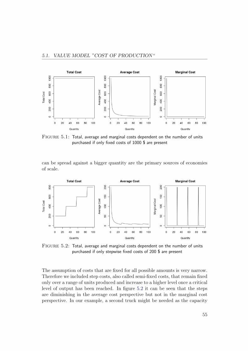
5.1. VALUE MODEL ”COST OF PRODUCTION“
Figure 5.1: Total, average and marginal costs dependent on the number of unitspurchased if only fixed costs of 1000 $ are present
can be spread against a bigger quantity are the primary sources of economiesof scale.
Figure 5.2: Total, average and marginal costs dependent on the number of unitspurchased if only stepwise fixed costs of 200 $ are present
The assumption of costs that are fixed for all possible amounts is very narrow.Therefore we included step costs, also called semi-fixed costs, that remain fixedonly over a range of units produced and increase to a higher level once a criticallevel of output has been reached. In figure 5.2 it can be seen that the stepsare diminishing in the average cost perspective but not in the marginal costperspective. In our example, a second truck might be needed as the capacity
55

CHAPTER 5. EXPERIMENTAL SETUP
of the first one is fully utilized.
5.1.1.2 Variable Cost
Variable costs on the other hand change, in proportion to the quantity thatis produced. In figure 5.3 we can see that linear variable costs on its own doproduce constant average and marginal cost. This can be interpolated easilywith a single price, both with incremental and total quantity discounts. In ourexample this could be the cost for the fuel used, which is linear in the weightof the truck.
Figure 5.3: Total, average and marginal costs dependent on the number of unitspurchased if only variable costs of 1 $ are present
In economics literature Pindyck and Rubinfeld (2005) average cost is generallythought to be U-shaped, because for low quantities the economies of scaledominate until an optimal point from where the diseconomies of scale becomedominant.
In our example variable costs could relate to the costs of the labor needed forhandling the goods transported. For amounts that can be handled by regularstaff in time it is decreasing, but when the capacity is fully utilized the costis increasing because of the overtime work. Variable costs therefore have apoint from whereon they grow faster than linear with the amount purchased.Together with fixed costs they combine to a U-shaped average cost functionas seen in figure 5.4. If there are not only superlinear variable cost presentbut also stepwise fixed costs the average total cost gets ”W“-shaped as seenin figure 5.5.
56

5.1. VALUE MODEL ”COST OF PRODUCTION“
Figure 5.4: Total, average and marginal costs dependent on the number of unitspurchased if fixed costs of 1000 $ and superlinear variable costs arepresent
Figure 5.5: Total, average and marginal costs dependent on the number of unitspurchased if stepwise fixed costs of 200 $ and superlinear variable costsare present
This makes the second derivative non-continuous and the approximation withvolume discounts hard. A possible way to avoid this, if the jumps in the costfunction are known, is to use lump sum markups.
57

CHAPTER 5. EXPERIMENTAL SETUP
5.1.2 Parametrizable Cost Function
In order to generate simulation instances we need to define a function thatcan on the one hand represent all the characteristics we have seen in theprevious section, and on the other hand it must be possible to parameterizeand repeatably randomize it.
5.1.2.1 Parametrizable Single Item Cost Function
We propose the following function to generate our instances with all availableparameters are summarized in table 5.1. Similar cost functions have been usedto estimate cost parameters of companies with multiple products or outputs(Baumol, 1987; Evans and Heckman, 1984; Stewart, 2009) in economics.
ci,s(xi,s) = Bi,sdxi,s/zi,se+ αi,sxi,s + βi,s(xi,s/γi,s)ρi,s
The first phenomenon we’ve seen are, possibly stepwise, fixed costs, which canbe distributed over an increasing number of goods for increasing demand, andlead to decreasing average costs. This is modeled by the first element andtherefore parameter of the cost function Bi,s. This describes the item specificstepwise fixed cost for item i,where z models the capacity bound, after whichan additional Bi,s of costs arise. Note, that with stepwise fixed costs present,the cost function is not continuous any more.
Cost function ParametersParameter DescriptionBi,s Item stepwise fixed cost of supplier s for item izi,s Capacity of production line for item i from supplier sαi,s Linear variable cost of supplier s for item iβi,s Slope of the nonlinear variable cost of supplier s for item iγi,s Delay of the nonlinear variable cost of supplier s for item iρi,s Exponent of the nonlinear variable cost of supplier s for item i
Table 5.1: Single item cost function parameters
The second phenomenon is the, possibly non-linear, variable cost. We haveincluded αi,s describing the linear part of the variable costs, though this pa-rameter is not by itself necessary in order to represent all the characteristics,
58

5.1. VALUE MODEL ”COST OF PRODUCTION“
because together with the fixed costs they allow different suppliers to be thecheapest at different demand levels.
βi,s describes the slope of the nonlinear part of the variable costs for producti and is also not indispensable but makes balancing between the fixed andvariable costs easier. ρi,s is the exponent of the nonlinear element in the costfunction, representing diseconomies of scale. The shape of the cost functionis very sensitive to this parameter and for values ≥ 1.3 it becomes dominanteven for moderate demand levels.
In practice we’ve seen the cost curves to be relatively flat and diseconomies ofscale to arise only for high demand levels but there quite sharp. In our costfunction this is made possible by γi,s which delays the effect of the nonlinearpart of the cost function. Problems instances with only a small flat proportionof near minimal average costs are not only unrealistic but also atypically easyto solve because large parts of the cost curves do not need to be considered.
5.1.2.2 Parametrizable Multi Item Cost Function
One of our key contributions is the possibility to include economies of scope andtherefore we also wanted to incorporate them into our experiments. The costfunction thereby must become a ”number of different good types”-dimensionalfunction, giving a cost for every possible combination of amounts of the goods.There are two main sources of economies of scope, shared fixed costs, andsynergies(similarities) between items. Both can be added easily to the singleitem cost function:
cs(x1, ..., xI) =
Asd∑i∈I
xi/Wie+∑i∈I
Bi,sdxi/zie+∑i∈I
βi,s(xi/γi,s)ρ +
∑i∈I
√xi∑i 6=j
χi,j,sxj
As describes the fixed overhead cost of supplier s and χi,j,s is used to modelsynergies between two products i and j. The term representing the synergiesis square rooted to make it a linear part of the cost function and can modelboth economies and diseconomies of scope with negative and positives valuesof χi,j,s. Table 5.2 gives a summary of all available parameters in the multiitem cost function.
Each of these parameters has to be chosen carefully in order not to degeneratethe resulting cost function.
59

CHAPTER 5. EXPERIMENTAL SETUP
Cost function ParametersParameter DescriptionAi,s Overhead cost of supplier sBi,s Item stepwise fixed cost of supplier s for item izi,s Capacity of production line for item i from supplier sαi,s Linear variable cost of supplier s for item iβi,s Factor of the nonlinear variable cost of supplier s for item iγi,s Delay of the nonlinear variable cost of supplier s for item iρi,s Exponent of the nonlinear variable cost of supplier s for item iχi,j,s Cross item cost synergy of supplier s for item i and j
Table 5.2: Multi item cost function parameters
5.1.2.3 Proposed Parametrization
Even the best parameterizable cost function will not generate meaningful testinstances if the parameters are not chosen carefully. For the related family ofknapsack problems it has been shown by Pisinger (2005) that the correlationbetween the weight and the profit of an item has a big impact on the hardnessof the problem.
Figure 5.6: Cost function base case (not randomized)
The equivalence of this correlation in our setting would be the correlationbetween the amount purchased and the costs for it. This maps to our obser-vation, that instances where there is a large relatively flat area in the averagecosts curves are harder. In figure 5.6 you can see the shape of the cost curve
60

5.1. VALUE MODEL ”COST OF PRODUCTION“
we used as a base case for our simulations. It includes all the properties we’vediscussed in section 5.1.1 and features a large relatively flat area in the averagecost. In table 5.3 you can see which parameters were used to generate this costcurve.
Variable Default valueBi,s 5000.0zi 33%αi,s 20.0βi,s 20.0γi,s 60.0ρ 15
Table 5.3: Parameters of the cost funtion in the proposed base case
On the other extreme instances that incorporate constant average costs aretrivial too, because then there are no payment modifiers needed to interpo-late the cost curve and the formulation becomes a linear program withoutintegrality constraints.
5.1.2.4 Randomization
In order to generate random problem instances out of this parameterizablecost function, the parameters need to be disturbed randomly. Here we needto be careful to balance between generating instances with sufficient variationand keeping the fundamental characteristics of the cost function.
The parameters for a randomized instance usually are drawn from a probabilitydistribution. By the central limit theorem, the sum of a number of randomvariables with finite means and variances approaches a normal distribution asthe number of variables increases.
The prices for a product are affected by a large number of factors that clearlyhave finite means and variances. Therefore we chose to draw all parametersfor the cost function of a specific instance from a normal distribution with themean being the base parameter as in table 5.3. The standard deviation wasset to values that gave a wide spectrum of shapes, but in average still yield a“W”-shaped cost function and are summarized in table 5.4.
For every parameter there was a plausibility check added, which prevented
61

CHAPTER 5. EXPERIMENTAL SETUP
inconsistent values and abolished the respecting instances. In figure 5.7 youcan see three examples of randomly parameterized cost functions.
Figure 5.7: Random instaces of the cost function for seeds 2,3 and 9
The similarity of the prices for equal amounts purchased from different sup-pliers is another important factor that needs to be considered. For real worldproducts the prices from different suppliers are clearly correlated through sim-ilar production standards and the market pressure nivellates disparities evenfurther.
In Leyton-Brown et al. (2002) the authors have shown that the number ofdominated bids is the key characteristic for the computational hardness of a
62

5.1. VALUE MODEL ”COST OF PRODUCTION“
Variable µ σitem σsupplierBi,s 5000.0 2500.0 500.0zi 33% 25% 15%αi,s 20.0 10.0 5.0βi,s 20.0 10.0 5.0γi,s 60.0 20.0 10.0ρ 15 2.0 0.5
Table 5.4: Parameters of the cost funtion in the base (singe item) case
combinatorial auction instance, and many distributions proposed in the litera-ture fail to generate a sufficient number of them. This leads to a misjudgmentof the problem size and interferes predictions of the running time. Analogouslyto the dominated bids in Leyton-Brown et al. (2002) cost curves that are dom-inated by other cost curves contain many payment modifiers that do not needto be considered.
As seen in figure 5.7 the shapes of the cost functions for different seeds arequite varying by design and a lot of them would be dominated if assigned tothe same item. Therefore we choose a two step process where we have drawnthe respective parameters for a cost curve per item. And in a second stepadded additional variation for each supplier taking the realization of the initialrandom variable as the mean of a new supplier-specific random variable. Therespective standard deviation values are shown in table 5.4 and three resultingsupplier specific cost curves are shown in figure 5.8.
The resulting cost curves together with the amount demanded already definethe optimal, meaning cost minimizing, solution of the problem. Translated intoa combinatorial auction instance, every possible combination of item amountsrequested would translate to a bid. The same would be possible in LESS byspecifying a payment modifier for every possible combination of item amountsrequested. This extreme approach clearly is a contradiction to our goal ofreducing the representation complexity for the bidders. Therefore the nextstep will be to derive rules how simulated bidders could interpolate their costfunction with the possibilities LESS offers.
63

CHAPTER 5. EXPERIMENTAL SETUP
Figure 5.8: Random instances of the cost function for seeds 2,3 and 9 anddifferent supplier realizations in dotted lines
5.2 Bid Generation
The bid generation describes the process of approximating the cost functionwith LESS , similar to what has been described in ??. The resulting functionwill be called bid interpolation function from here on.
Note, that in a real procurement auction suppliers might not want to reveal
64
5.2. BID GENERATION
their true cost functions if it is not induced by the auction mechanism. Forcombinatorial auctions this can be reached by a so called generalized vickeyauction for example as described in 2.2.2.1. Note further, that if the approx-imation error gets large and the bid language does not allow to describe theunderlying cost function arbitrarily close, this might have an impact on thebidding strategy and bidders might have an incentive to speculate.
The applicability or transformability of this mechanism to our problem wouldbe an interesting further work and is not examined in this thesis. A gametheoretical analysis only makes sense if we already have a working biddinglanguage and supplier selection process, and therefore we assume well behavingbidders to evaluate the possible performance of our approach.
Accordingly we assume a direct revelation mechanism, where bidders try to re-veal bids reflecting the underlying total cost function truthfully and as close aspossible without underbidding their costs. We analyze two treatments: Eitherthe number of discounts per item and the corresponding quantity intervals arefixed, or the suppliers can supply an arbitrary number of intervals determinedby a predefined approximation error εmaxs .
5.2.1 Fixed Interval Bidding
Often in practical settings the boundaries of the price intervals are predefinedby the auction, as this only requires the bidders to submit a single numberper interval indicating the price valid in that interval. This also can be easilyimplemented in a web form for example.
Predefining the intervals naturally limits the expressiveness of the bidding lan-guage. In figure 5.9 you can see the bid interpolation functions of our standardcost function without stepwise fixed costs using five equidistant intervals forincremental and total quantity bids.
For total quantity bids, where the resulting interpolation function is piece-wise linear in the intervals, one can see, that the bid interpolation functionoverlaps with the cost function at the point of maximal average costs. Astotal quantity bids describe a piecewise constant function in average costs thispoint determines the minimal price at which the interpolation function neverlies below the cost function. As for total quantity discounts the price is validfor the whole amount purchased, the resulting interpolation function intersectsthe origin of the coordinate system in total costs, resulting in the typical saw
65

CHAPTER 5. EXPERIMENTAL SETUP
Figure 5.9: Comparison of fixed interval bidding with 5 intervals
tooth shape. The approximation error increases with an increasing gradient ofthe average cost curve.
With incremental bids on the other hand the price is valid only for the incre-mental units and the total cost curve of the bid interpolation function dos notincorporate any jumps. The resulting bid interpolation function is constanton marginal costs and the approximation error depends on the gradient of themarginal cost curve. As discussed in ?? the approximation error of incrementalbids is never greater than the approximation error of total quantity bids forconvex cost functions.
If the cost function itself does incorporate jumps, as generated by stepwisefixed costs for example, this does no longer hold for all cases. The jumps intotal cost effects that the bid interpolation function for incremental bids doesno longer overlap with the cost function at the interval boundaries. Thereforethe approximation error can get arbitrarily big if a jump occurs close to aninterval boundary. Total quantity bids do not suffer from this effect but theinterpolation error also tends to increase with the presence of stepwise fixedcosts on a smaller scale.
66

5.2. BID GENERATION
Figure 5.10: Comparison of fixed interval bidding with 5 intervals and stepwisefixed costs
5.2.2 Fixed Approximation Error Bidding
The intention of LESS was to make it handle able for bidders to express theircost function by reducing the number of priced needed. Therefore we investi-gated the question how many priced are needed to express a cost function withan bounded approximation error and which impact has this on computationtime and total spend.
To answer this question we implemented a simulated bidding agent that inter-polates a given cost function with a given approximation error using as littletiers as possible. It features greedy approach that generates maximally wideintervals regarding the tolerable approximation error relative to the currenttotal costs, starting at a single item. In 5.11 you can see the resulting bidapproximation functions.
The large approximation errors for incremental bids with fixed intervals arecaused by disadvantageous interval boundaries. If bidders can define the pricebreaks freely, as in LESS, a jump in the cost function can be interpolated withan incremental markup followed by an incremental discount. The jump intotal cost translates to a spike in marginal costs, which can be interpolatedwith an incremental interval of length 1.
67

CHAPTER 5. EXPERIMENTAL SETUP
Figure 5.11: Comparison of fixed approximation error bidding with a maximumerror of 25%
For total quantity bidding the advantage of having freely settable price rangesis not as outstanding but it allows the bidders to express their costs func-tions as close as desired. For both discount types having freely settable priceranges allows to interpolate any given cost function exactly by defining a priceindividually for every possible quantity.
68

5.2. BID GENERATION
5.2.2.1 Fixed Approximation Error Bidding with Lump Sum Mod-ifiers
As pointed out in 5.1.1 jumps in the cost function cannot only be expressed asa pair of an incremental discount and markup in LESS, but also by so calledlump sum markups. If lump sum markups are used to express jumps the netcost function is convex again and incremental bidding reduces to piecewiselinear interpolation as described in ??.
Figure 5.12: Comparison of fixed approximation error bidding with a maximumerror of 25% without fixed costs
In figure 5.12 you can see the approximation of our standard cost functionwhere the fixed costs set to zero. This reflects the situation a bidder faces ifthe fixed costs are already covered using lump sum markups. With no fixedcosts present the average costs are strictly increasing. Therefore there are forincremental bidding only markups needed to describe the nonlinearity at highamounts. For total quantity bidding the situation even improves more as theapparent absence of fixed costs makes the total cost function go through theorigin of the coordinate system.
69

CHAPTER 5. EXPERIMENTAL SETUP
70

Chapter 6
Experimental Results
In this chapter we will summarize the results of our simulation experiments.
6.1 Cost of Flexibility
Goossens et al. (2007) provided a tailor-made formulation for total quantitydiscount bids, as well as computational results on randomly generated testinstances. In contrast, LESS provides bidders with more flexibility and allowsfor other types of volume discounts and various spend conditions. Typically,more flexibility and expressiveness comes at the cost of computational com-plexity. It is interesting to see, if the expressiveness of LESS comes at a largecomputational cost.
Therefore, in a first set of experiments, we used the synthetic bids, which werekindly provided by Goossens et al. (2007) for a comparison. These experimentsare limited to bids with total quantity discounts only.
In their instances with 40 items, Goossens et al. (2007) generated anupperbound-increase from one interval to the next, which was a random num-ber between 10,000 and 50,000, while for instances with 100 items, the up-perbound increase was a random number between 10,000 and 100,000. Theresults of the formulation in Goossens et al. (2007) with a branch-and-cut ap-proach and with the SQS formulation can be found in Tables 6.1 and 6.2. Wefocus on the branch-and-cut results, since those provided the best results forlarger instances. Note that we have used CPLEX version 12.1, while Goossens
71

CHAPTER 6. EXPERIMENTAL RESULTS
SQS b&c Goossens b&cInstances comp. time #nodes comp. time #nodesS 10 40 3 0.08 9.3 0.09 0.3S 10 40 5 0.17 16.4 0.15 10.9S 10 100 3 0.13 5 0.12 0.2S 10 100 5 1.13 31.1 0.55 3.2
S 20 40 3 0.16 10.9 0.12 0.5S 20 40 5 0.87 36.7 0.50 4.7S 20 100 3 0.49 17.1 0.34 2.1S 20 100 5 2.40 32.1 1.17 2.1
S 50 40 3 0.79 34.6 0.51 2.7S 50 40 5 5.87 102.9 2.99 16.5S 50 100 3 2.45 28.0 1.45 2.1S 50 100 5 21.67 94.8 10.45 14.7
R 10 40 3 0.07 6.7 0.09 2.1R 10 40 5 1.10 85.5 0.59 30.5R 10 100 3 0.22 7.2 0.14 2.6R 10 100 5 3.814 70.8 1.50 31.7
R 20 40 3 0.29 18.7 0.29 9.5R 20 40 5 3.76 138.5 1.81 68.5R 20 100 3 1.41 25.9 0.83 8.1R 20 100 5 29.75 274.9 6.81 70.1
R 50 40 3 2.01 71.3 1.67 81.6R 50 40 5 26.90 346.5 14.18 140.9R 50 100 3 12.75 91.9 8.84 43.8R 50 100 5 451.84 996.0 61.71 216.8
Table 6.1: Comparison of SQS against the results by Goossens et al. (2007) (basecase)
et al. (2007) used version 8.1. Also, they used a Pentium IV 2 GHz computerwith 512 Mb RAM. Nevertheless, the comparison helps understand possiblepenalties for a more expressive bidding language.
72

6.1. COST OF FLEXIBILITY
SQS b&c Goossens b&cInstances comp. time #nodes comp. time #nodesS 10 40 3 0.05 6.2 0.14 0.4S 10 40 5 0.16 12.6 0.49 23.2S 10 100 3 0.09 2.1 0.29 6.8S 10 100 5 1.05 26.4 2.48 66.5
S 20 40 3 0.12 8.9 0.45 5.2S 20 40 5 0.87 31.9 4.42 148.7S 20 100 3 0.44 11.1 2.08 43.4S 20 100 5 2.08 28.8 11.47 164.2
S 50 40 3 0.61 19.4 8.90 261.9S 50 40 5 6.02 100.6 147.56 2500.0S 50 100 3 2.17 20.4 28.42 523.7S 50 100 5 21.02 84.7 271.80 3006.0
R 10 40 3 0.07 6.3 0.10 0.1R 10 40 5 0.71 40.7 0.67 18.5R 10 100 3 0.19 7.5 0.17 0.2R 10 100 5 3.19 51.5 2.49 42.6
R 20 40 3 0.24 12.8 0.60 15.9R 20 40 5 2.64 80.7 3.55 89.8R 20 100 3 1.07 21 1.85 17.6R 20 100 5 31.38 322 25.09 434.8
R 50 40 3 1.65 49.1 35.16 1196.8R 50 40 5 21.82 298.7 169.82 1511.1R 50 100 3 10.78 68.6 274.82 6035.4R 50 100 5 400.68 1064.3 2036.07 17577.4
Table 6.2: Comparison of SQS against the results in Goossens et al. (2007) (morefor less)
Interestingly, much larger instances could be solved to optimality with this setof bids in seconds, and the differences in runtime between the results reportedby Goossens et al. (2007) and the results of SQS were small. The results for
73

CHAPTER 6. EXPERIMENTAL RESULTS
the base case in Table 6.1 where a bit slower, while the results for the more-for-less scenario in Table 6.2 were actually faster. The more-for-less scenarioaimed for optimal solutions with free disposal of additional quantity, while thebase case did not.
Obviously, the structure of the bids has a significant impact on the runtime.The bids generated based on our multi-product cost function were considerablyharder to solve. We assume that smooth cost functions generate a lot ofsolutions with similar objective function value, a type of symmetry problem.The structured instances in Goossens et al. (2007) include economies of scale,where intervals with more quantity have lower prices than intervals with lessquantity, whereas the cost functions in our paper also include diseconomies ofscale. Also the demand can make a difference. If the demand is increased,runtimes can increase, because there are more possible quantities to purchase.
In summary, the predictive quality of such runtime experiments depends on thestructure of the bids and the respective scale economies in a market. Overall,our analysis reveals that surprisingly large instances can be solved to optimalitywith these types of bids.
74
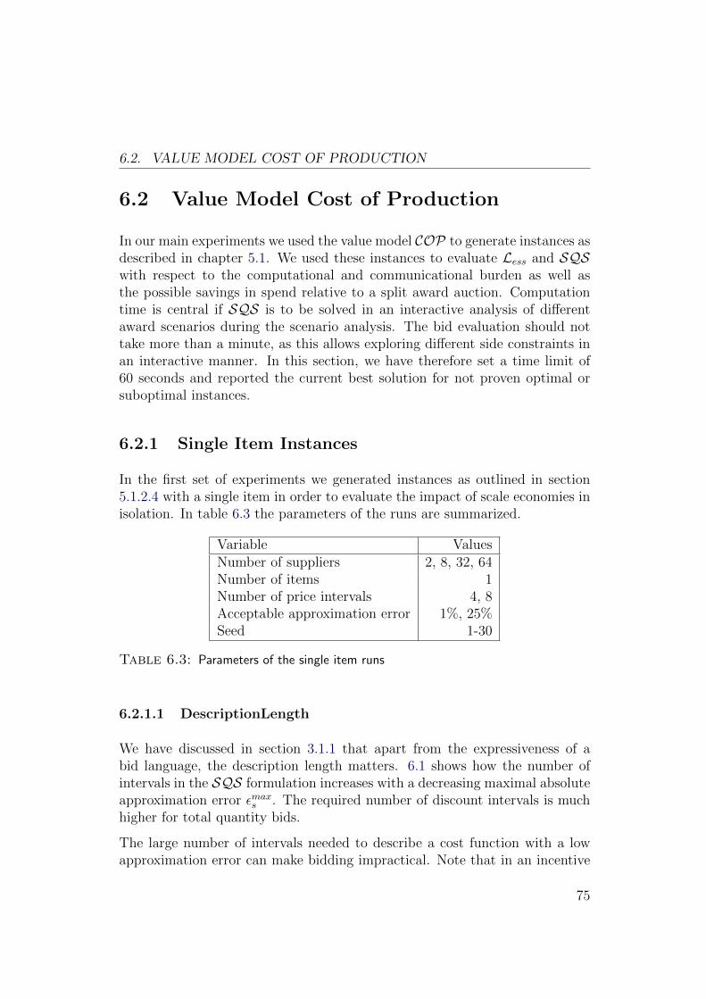
6.2. VALUE MODEL COST OF PRODUCTION
6.2 Value Model Cost of Production
In our main experiments we used the value model COP to generate instances asdescribed in chapter 5.1. We used these instances to evaluate Less and SQSwith respect to the computational and communicational burden as well asthe possible savings in spend relative to a split award auction. Computationtime is central if SQS is to be solved in an interactive analysis of differentaward scenarios during the scenario analysis. The bid evaluation should nottake more than a minute, as this allows exploring different side constraints inan interactive manner. In this section, we have therefore set a time limit of60 seconds and reported the current best solution for not proven optimal orsuboptimal instances.
6.2.1 Single Item Instances
In the first set of experiments we generated instances as outlined in section5.1.2.4 with a single item in order to evaluate the impact of scale economies inisolation. In table 6.3 the parameters of the runs are summarized.
Variable ValuesNumber of suppliers 2, 8, 32, 64Number of items 1Number of price intervals 4, 8Acceptable approximation error 1%, 25%Seed 1-30
Table 6.3: Parameters of the single item runs
6.2.1.1 DescriptionLength
We have discussed in section 3.1.1 that apart from the expressiveness of abid language, the description length matters. 6.1 shows how the number ofintervals in the SQS formulation increases with a decreasing maximal absoluteapproximation error εmaxs . The required number of discount intervals is muchhigher for total quantity bids.
The large number of intervals needed to describe a cost function with a lowapproximation error can make bidding impractical. Note that in an incentive
75
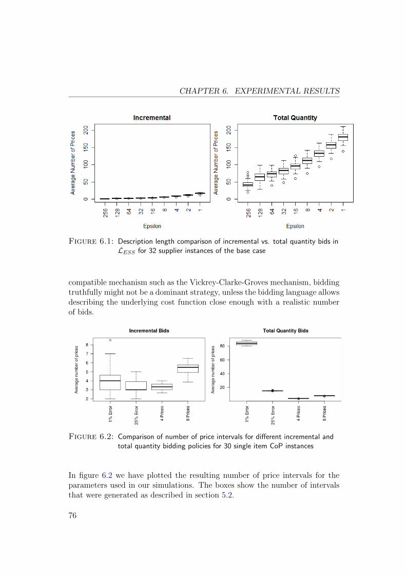
CHAPTER 6. EXPERIMENTAL RESULTS
Figure 6.1: Description length comparison of incremental vs. total quantity bids inLESS for 32 supplier instances of the base case
compatible mechanism such as the Vickrey-Clarke-Groves mechanism, biddingtruthfully might not be a dominant strategy, unless the bidding language allowsdescribing the underlying cost function close enough with a realistic numberof bids.
Figure 6.2: Comparison of number of price intervals for different incremental andtotal quantity bidding policies for 30 single item CoP instances
In figure 6.2 we have plotted the resulting number of price intervals for theparameters used in our simulations. The boxes show the number of intervalsthat were generated as described in section 5.2.
76

6.2. VALUE MODEL COST OF PRODUCTION
For incremental bidding the necessary number of price intervals was alwaysbelow ten even with an approximation error of 1 %. For total quantity biddingon the other hand, even an approximation error of 25 % demanded around 20price intervals. This shows, the burden for the bidders to communicate theircost function nearly exactly is only manageable using incremental bids in thesesettings.
6.2.1.2 Computational Burden
In figures 6.3, 6.4 and 6.5 one can see a comparison of the computation timeneeded to solve SQS for instances with 2, 8 and 64 suppliers and for differentbidding policies.
Figure 6.3: Comparison of computation time for different incremental and totalquantity bidding policies for 30 single item CoP instances with 2suppliers
The number of intervals greatly influences the expected computation time forSQS, which can be clearly seen in our results. All instances except the oneswith total quantity bids and an approximation error limiting bidding policycould be solved to proven optimality within 60 seconds. With an allowedapproximation error of 25 % only a few instances timed out, whereas with anallowed approximation error of 1% and at least 8 suppliers more than half ofthe instances timed out.
The instances with a fixed number of price intervals could all be solved tooptimality in less than 20 seconds. At four price levels total quantity instances
77
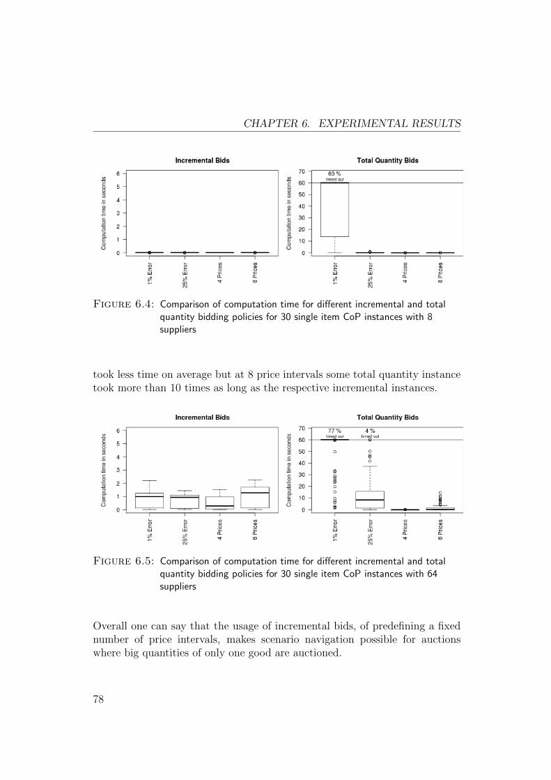
CHAPTER 6. EXPERIMENTAL RESULTS
Figure 6.4: Comparison of computation time for different incremental and totalquantity bidding policies for 30 single item CoP instances with 8suppliers
took less time on average but at 8 price intervals some total quantity instancetook more than 10 times as long as the respective incremental instances.
Figure 6.5: Comparison of computation time for different incremental and totalquantity bidding policies for 30 single item CoP instances with 64suppliers
Overall one can say that the usage of incremental bids, of predefining a fixednumber of price intervals, makes scenario navigation possible for auctionswhere big quantities of only one good are auctioned.
78
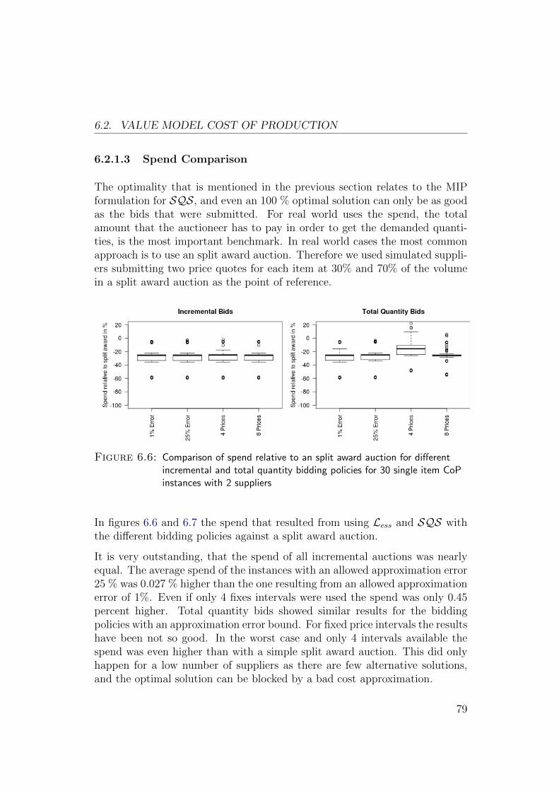
6.2. VALUE MODEL COST OF PRODUCTION
6.2.1.3 Spend Comparison
The optimality that is mentioned in the previous section relates to the MIPformulation for SQS, and even an 100 % optimal solution can only be as goodas the bids that were submitted. For real world uses the spend, the totalamount that the auctioneer has to pay in order to get the demanded quanti-ties, is the most important benchmark. In real world cases the most commonapproach is to use an split award auction. Therefore we used simulated suppli-ers submitting two price quotes for each item at 30% and 70% of the volumein a split award auction as the point of reference.
Figure 6.6: Comparison of spend relative to an split award auction for differentincremental and total quantity bidding policies for 30 single item CoPinstances with 2 suppliers
In figures 6.6 and 6.7 the spend that resulted from using Less and SQS withthe different bidding policies against a split award auction.
It is very outstanding, that the spend of all incremental auctions was nearlyequal. The average spend of the instances with an allowed approximation error25 % was 0.027 % higher than the one resulting from an allowed approximationerror of 1%. Even if only 4 fixes intervals were used the spend was only 0.45percent higher. Total quantity bids showed similar results for the biddingpolicies with an approximation error bound. For fixed price intervals the resultshave been not so good. In the worst case and only 4 intervals available thespend was even higher than with a simple split award auction. This did onlyhappen for a low number of suppliers as there are few alternative solutions,and the optimal solution can be blocked by a bad cost approximation.
79

CHAPTER 6. EXPERIMENTAL RESULTS
Figure 6.7: Comparison of spend relative to an split award auction for differentincremental and total quantity bidding policies for 30 single item CoPinstances with 64 suppliers
6.2.2 Single Item Instances with Lump Sum Discountsand Markups
In Less suppliers have the option to define so called lump sum discountsand markups, that are a one time payment. These lump sum discounts andmarkups can be interpreted as a direct way to communicate jumps in the costfunction, as illustrated in section 5.2.2.1. In practice the bidders will only veryseldom be able and or willing to communicate this information so this is moreof theoretical value.
In figure 6.8 one can see, that the use of lump sum markups to indicate thejumps in the cost function makes computing SQS faster, and all instancescould be solved in less than a second. Figure 6.9 shows the spend if biddersuse lump sum markups. For all error bound bidding policies the spend waswithin less than 0.1 % of the optimum. With incremental bids 4 price intervalswere also sufficient to get close to the optimal spend, and also total quantitybids profited a lot.
80

6.2. VALUE MODEL COST OF PRODUCTION
Figure 6.8: Comparison of computation time for different incremental and totalquantity bidding policies for 30 single item CoP instances with 64suppliers
Figure 6.9: Comparison of spend relative to a split award auction for differentincremental and total quantity bidding policies using lump sumdiscounts and markups for 30 single item CoP instances
6.2.3 Multi Item Instances - Realistic Problems
Finally, we will discuss the impact of the different discount policies on thetotal cost of the purchasing organization when auctioning multiple items atonce. This is the most realistic but also most challenging scenario for thebidding language and supplier selection. In contrast to the single item caseswhere we focused on elaborating effects scale economies on bidding and supplier
81

CHAPTER 6. EXPERIMENTAL RESULTS
selection, we tried here to explore the applicability of Less and SQS for realisticmulti item instances.
Again, we assume a direct revelation mechanism, and bidders submit theirbid in a way that approximates their true costs as close as possible, eitherrestricted by the number of intervals or a predefined approximation error. Wesimulated suppliers submitting two price quotes for each item at 30% and 70%of the volume in a split-award auction using the value model cost of productionwith parameters outlined as 5.1.2.4. The same suppliers also submit bids inan auction with only total quantity discount bids, and in an auction with onlyincremental volume discount bids. For the latter two auction types, we alsodistinguished settings with a fixed set of 5 intervals, or an approximation errorε of 1.0 %.
The results are summarized in Table 6.4. Each row summarizes the result ofa particular volume discount auction relative to the cost of the split-awardauction in percentage values after 5, 10, 20, 60, 120, and 500 seconds. Allreported numbers are average numbers for 30 instances solved.
A spend greater than the one that could be realized by an split award auctioncan be a result of two factors, either the interpolation error is too big or thecurrent integer solution is too far away from the optimum. Therefore we havethen analyzed the proven optimality of these instances, and the MIP gap after5, 10, 20, 60, 120 and 500 seconds can be found in 6.5. A value of −1.000means that the best bound found so far is still ≤ 0, and there is no meaningfulMIP gap reported by the solver.
As one can see the incremental instances with 5 intervals were not solved tooptimality, while the instances with total quantity discounts could be solvedto optimality even for larger instances with 30 suppliers and 10 items in 2minutes. So the MIP gap of the incremental volume discount bids was alwayshigher, when the number of intervals was limited to five. With a limit on theapproximation error ε to 1%, the number of intervals grows up to more than 80intervals per item in case of total quantity discount bids, but only up to around30 intervals in case of volume discount bids. Interestingly, the instances withonly incremental volume discount bids are still harder to solve and the MIPgap is typically larger. So, the structure of the problems with total quantitydiscounts allows for larger problems to be solved.
We will now take a look at the spend with a fixed number of 5 intervals. If theMIP gap is high, then also the spend with total quantity discount bids andincremental volume discount bids can be much worse than with simple split
82

6.2. VALUE MODEL COST OF PRODUCTION
Spend in % of split awards with time limitSuppliers Items 5s 10s 20s 60s 120s 500sTotal quantity 5 intervals10 10 101.13 100.94 100.94 100.02 100.94 100.9410 30 101.22 101.22 101.22 101.58 101.22 101.2210 50 102.28 102.20 102.19 102.45 102.19 102.1930 10 101.44 101.44 101.44 101.44 101.44 101.4430 30 102.75 102.59 102.57 103.80 102.56 102.5630 50 102.79 102.69 102.48 102.74 102.27 102.27Incremental 5 intervals10 10 93.65 93.47 93.49 93.27 93.45 93.4610 30 97.31 95.50 94.67 94.84 94.48 94.4010 50 103.54 100.72 96.70 95.87 95.62 95.4630 10 96.76 94.86 94.37 92.63 94.28 94.2130 30 109.45 109.09 105.02 97.81 95.97 95.6230 50 115.53 113.37 107.40 103.07 97.98 95.85Total quantity ε = 1.010 10 93.59 93.60 93.60 93.52 93.25 87.8910 30 29311.83 95.37 95.37 95.77 95.36 95.1710 50 31571.88 29585.34 96.65 97.44 96.64 96.6430 10 117653.66 97.36 97.34 96.49 97.36 96.9630 30 92869.85 92869.85 92869.85 102.60 102.30 102.2930 50 82807.65 83589.52 83589.52 92582.93 103.08 103.08Incremental ε = 1.010 10 87.72 87.73 86.35 86.09 86.27 86.1510 30 374.71 132.40 94.47 90.68 88.08 87.6910 50 450.39 335.86 123.02 95.08 89.94 89.1930 10 930.91 184.22 96.96 89.46 87.88 87.2930 30 1449.13 1277.17 1350.74 162.00 103.73 90.9730 50 1675.84 1433.83 1333.95 696.10 150.84 94.08
Table 6.4: Comparison of spend relative to a split award auciton
award auctions. Therefore, we will mainly look at the column with 500s, wherethe MIP gap was low. Interestingly, in the setting with total quantity bids and5 intervals, the spend achieved was higher than that of split award auctions,although the smaller instances could be solved to optimality. The reason forthis is the bad approximation. In contrast, incremental volume discount bids
83

CHAPTER 6. EXPERIMENTAL RESULTS
Optimality with time limitSuppliers Items Prices 5s 10s 20s 60s 120s 500sTotal quantity, 5 intervals10 10 5 1.000 1.000 1.000 1.000 1.000 1.00010 30 5 1.000 1.000 1.000 1.000 1.000 1.00010 50 5 0.997 0.998 0.999 0.999 1.000 1.00030 10 5 1.000 1.000 1.000 1.000 1.000 1.00030 30 5 0.993 0.996 0.997 0.998 0.998 0.99830 50 5 0.989 0.991 0.993 0.996 0.996 0.997Incremental, 5 intervals10 10 5 0.937 0.944 0.947 0.963 0.958 0.96510 30 5 0.890 0.909 0.919 0.927 0.923 0.92610 50 5 0.844 0.867 0.904 0.918 0.916 0.92030 10 5 0.887 0.909 0.916 0.925 0.921 0.92730 30 5 0.438 0.765 0.802 0.877 0.881 0.88930 50 5 0.319 0.512 0.765 0.804 0.840 0.866Total quantity ε < 1.010 10 80.41 0.636 0.680 0.725 0.775 0.812 0.86810 30 77.36 -1.000 0.509 0.558 0.638 0.681 0.75810 50 76.65 -1.000 -1.000 0.496 0.582 0.615 0.69930 10 80.41 -1.000 0.515 0.584 0.646 0.693 0.76030 30 77.36 -1.000 -1.000 -1.000 0.493 0.529 0.62130 50 76.92 -1.000 -1.000 -1.000 0.000 0.441 0.549Incremental ε < 1.010 10 28.20 0.595 0.811 0.880 0.937 0.911 0.94610 30 25.28 -1.000 0.219 0.375 0.412 0.538 0.59710 50 24.58 -1.000 -1.000 0.328 0.438 0.499 0.57630 10 28.20 -1.000 -1.000 -1.000 -1.000 0.096 0.16830 30 25.22 -1.000 -1.000 -1.000 -1.000 -1.000 0.10830 50 24.52 -1.000 -1.000 -1.000 -1.000 -1.000 -1.000
Table 6.5: Proven optimality of the solutions in table 6.4
achieved a lower total cost compared to split award auctions for all problemsizes already after 120 seconds. This was the case, even though the problemscould not be solved to optimality within 500 seconds.
In situations, where the approximation error ε was limited to 1%, total quantity
84

6.2. VALUE MODEL COST OF PRODUCTION
discount bids led to cost savings after 500 seconds compared to split-awardauctions. Larger instances with 30 suppliers and 30 items led to a large MIPgap even after 500 seconds and the results were worse than those of a splitaward auction. Also in this setting, the incremental volume discounts led tolower total cost compared to split-award auctions for all problem sizes, butalso compared to total quantity discount bids after 500 seconds.
85

CHAPTER 6. EXPERIMENTAL RESULTS
86

Chapter 7
Conclusion and Outlook
7.1 Conclusion
We have suggested a bidding language for markets with economies of scale andscope and a respective MIP to solve the resulting supplier quantity selection(SQS) problem. We try to easy the problematic bidding complexity, induced bythe huge number of possible bid combinations, for the bidders in a combintorialauction. This problem we’ve shown, by numerical simulations, to be a limitingfactor of the performance of combinatorial auctions in general. This gets evenworse in procurement settings.
The proposed bidding language is considerably more expressive than what hasbeen discussed in the literature so far and includes incremental volume dis-counts, total quantity discounts, lump sum discounts, and a variety of spendconditions defined on spend and quantity of selected items. While both, in-cremental volume discount bids and total quantity discount bids, have beendescribed in the literature and are used in procurement practice, there has notbeen a thorough comparison among those discount policies as of yet. This isthe first paper, to use different types of cost functions to generate bids, whichallowed us to analyze not only computation times, but also total spend ofdifferent discount policies.
Our results show that that realistic problem sizes can be solved in a matterof minutes, but that big multi item problems with only incremental volumediscount bids are harder to solve than those with only total quantity discountbids. On the other hand if a supplier wants to approximate his true cost
87

CHAPTER 7. CONCLUSION AND OUTLOOK
function with total quantity discount bids closely, this leads to a much largerand number of discount intervals.
There were several situations, where the results of simple split-award auctionswith simple price quotes lead to lower total cost than those of more advancedbidding languages. The reason is either a bad approximation of the costs or theinability to find the cost-minimal solution within an acceptable response time.For example, if suppliers only used a few total quantity discount intervals, thisled to much higher total cost for the buyer. However, we have also shown thatsignificant savings can be achieved with compact bidding languages comparedto split award auctions, if bidders are able to approximate their cost functionswell. Even though big instances with few incremental price intervals could notbe proven to be optimal, the resulting costs were always lower than the onesresulting of a split award auction.
In summary, a procurement manager needs to take care that the bidding lan-guage provides enough flexibility so that bidders can describe their cost struc-tures arbitrarily close. At the same time bids should have low descriptionlength, such that suppliers are only forced to specify a few parameters and nothundreds of numbers. Also, a procurement manager should make sure thatthe number of bids in an application is such that he can expect to solve theproblem instances to optimality. The results of our analysis should provide abetter understanding under which circumstances compact bidding languagesshould be used in procurement practice. Mechanism design questions havebeen outside the scope of this paper, and remain fruitful questions for futureresearch in this area.
While the bid language leads to much flexibility for the suppliers in specify-ing discounts in a compact format, it also incurs computational complexityon the buyer’s side. Practical applications span a wide range of possible com-putational time requirements ranging from demanding interactive uses suchas scenario analysis, and dynamic reverse auctions where acceptable compu-tational times may be in the scale of minutes, to less demanding cases suchas multiple round negotiations where runtimes in hours, often days, may betolerable. We have analyzed the empirical hardness of SQS and the time tosolve various problem sizes in order to understand the impact of different typesof constraints and discounts on the runtime with a focus on interactive appli-cations such as scenario analysis.
The results provide an understanding under which circumstances such expres-sive bidding languages can be used in procurement practice. We have also
88
7.2. OUTLOOK
analyzed the potential impact of such bidding languages on the total spendof the purchasing manager, if bidders reveal their costs truthfully, and foundthat the cost savings depend on the parameters of the cost function and thebidding language used.
7.2 Outlook
Our main goal was to improve the performance of procurement auctions bygiving the suppliers a better possiblity to express their costs, and the therbylowering the costs for the buyer, together with provinding a better understand-ing of the scenario. With our computational experiments we haven shown thefeasibility of our aproach in priciple, but real events always incorporate humanbidders, and therefore a verification of our results by lab experiments remainsan important open issue.
Mechanism design questions have been out of the scope of this work and wehave assumed extremely well behaving bidders, which clearly is a very strongassumption. A game theoretical analysis of the proposed mechanism couldtherefore provide valueable insights how bidders might behave in such a pro-curement event.
The capability of the bidders to express their cost, is crucial as we have seen,and could greatly benefit from a visual representation of their bids. The useof total quantity bidding is still dominating in real procment events, as theyseem to appear easier to grasp in textual form. Already a very simple plot ofthe resulting costs, as for example as in section 5.2, could help in promotingthe use of incremental discounts in our opinion, as they would demonstratethe resulting jumps in the cost function.
In iterative combinatorial auctions the bidders gain feedback in between roundsby the form of ask prices and can improve their bids accordingly. In practicalsettings further guidance of the bidders is necessary as Scheffel et al. (2010)have shown in their analysis of linear price auctions and therein also importanceof bidder decision support. For combinatorial auctions we have seen thatthe simpler linear price auctions can perform very good, in contrast to theirtheoretical limitations.
In section 4.2.1 we have suggested a simple price feedback based on a lumpsum discount request. It remains an interesting question if such a very simplefeedback, that has the advantage of a very easy and fast comprehensiveness,
89

CHAPTER 7. CONCLUSION AND OUTLOOK
could guide the buyers accordingly in an iterative action based on Less andSQS.
90

Bibliography
Abrache, Jawad, Benoıt Bourbeau, Teodor Gabriel Crainic, Michel Gendreau.2004. A new bidding framework for combinatorial e-auctions. Computers &Operations Research 31(8) 1177–1203.
Adomavicius, G., A. Gupta. 2005. Towards comprehensive real-time biddersupport in iterative combinatorial auctions. Information Systems Research(ISR) 16 169–185.
An, N., W. Elmaghraby, P. Keskinocak. 2005. Bidding strategies and their im-pact on revenues in combinatorial auctions. Journal of Revenue and PricingManagement .
Ausubel, L., P. Cramton, P. Milgrom. 2006. The clock-proxy auction: A prac-tical combinatorial auction design. P. Cramton, Y. Shoham, R. Steinberg,eds., Combinatorial Auctions . MIT Press, Cambridge, MA.
Ausubel, L., P. Milgrom. 2006a. Ascending proxy auctions. P. Cramton,Y. Shoham, R. Steinberg, eds., Combinatorial Auctions . MIT Press, Cam-bridge, MA.
Ausubel, L., P. Milgrom. 2006b. The lovely but lonely vickrey auction.P. Cramton, Y. Shoham, R. Steinberg, eds., Combinatorial Auctions . MITPress, Cambridge, MA.
Baumol, W. J. 1987. Microtheory: Applications and Origins . 1st ed. MITPress, Cambridge, MA, USA.
Benisch, M., N. Sadeh, T. Sandholm. 2008. A theory of expressiveness inmechanisms. 23rd AAAI Conference on Artificial Intelligence.
Bichler, M., A. Davenport, G. Hohner, J. Kalagnanam. 2006. Industrial pro-curement auctions. P. Cramton, Y. Shoham, R. Steinberg, eds., Combina-torial Auctions . MIT Press.
91
BIBLIOGRAPHY
Bichler, M., J. Kalagnanam. 2005. Configurable offers and winner determina-tion in multi-attribute auctions. European Journal of Operational Research160(2) 380–394.
Bichler, M., J. Kalagnanam, K. Katircioglu, A. King, R. Lawrence, H. Lee,G. Lin, Y. Lu. 2002. Applications of flexible pricing in business-to-businesselectronic commerce. IBM Systems Journal 41 287–302.
Bichler, M., P. Shabalin, A. Pikovsky. 2009. A computational analysis of linear-price iterative combinatorial auctions. Information Systems Research 20(1)33–59.
Bikhchandani, S., J. M. Ostroy. 2002. The package assignment model. Journalof Economic Theory 107(2) 377–406.
Blumrosen, L., N. Nisan. 2005. On the computational power of iterativeauctions. ACM Conference on Electronic Commerce (EC 05). Vancouver,Canada.
Boutilier, C., H. H. Hoos. 2001. Bidding languages for combinatorial auctions.17th International Joint Conference on Artificial Intelligence (IJCAI) 2001 .Washington, USA, 1211–1217.
Chandru, V., J. Hooker, eds. 1999. Optimization Methods for Logical Inference.John Wiley & Sons.
Chaudhry, S., F. Forst, J. L. Zydiak. 1993. Vendor selection with price breaks.European Journal of Operaitonal Research 70 52–66.
Chen, Yan, Kan Takeuchi. 2009. Multi-object auctions with package bidding:An experimental comparison of vickrey and ibea. Games and EconomicBehavior to appear –. doi:10.1016/j.geb.2009.10.007.
Crama, Y., R. Pascual, A. Torres. 2004. Optimal procurement decisions inthe presence of total quantity discounts and alternative product recipes.European Journal of Operational Research 159 364–378.
Cramton, P., Y. Shoham, R. Steinberg. 2006. Introduction to combinatorialauctions. P. Cramton, Y. Shoham, R. Steinberg, eds., Combinatorial Auc-tions . MIT Press, Cambridge, MA.
92

BIBLIOGRAPHY
Dang, V., N. Jennings. 2003. Optimal clearing algorithms for multi-unit single-item and multi-unit combinatorial auctions with demand-supply functionbidding. Technical report, Dept. of Electronics and Computer Science, Univ.of Southampton, UK.
Davenport, A., J. Kalagnanam. 2000. Price negotiations for procurement ofdirect inputs. IMA Hot TopicsWorkshop: Mathematics of the Internet: E-Auction and Markets , vol. 127. Minneapolis, USA, 27–44.
de Vries, S., J. Schummer, R. Vohra. 2007. On ascending vickrey auctions forheterogeneous objects. Journal of Economic Theory 132 95–118.
Dunford, M., K. Hoffman, D. Menon, R. Sultana, T. Wilson. 2007. Testinglinear pricing algorithms for use in ascending combinatorial auctions. Tech.rep., George Mason University.
Eso, M., S. Ghosh, J. Kalagnanam, L. Ladanyi. 2001. Bid evaluation in pro-curement auctions with piece-wise linear supplycurves. Technical reportrc22219, IBM T.J. Watson Research Center.
Evans, D., J. Heckman. 1984. A test for subadditivity of the cost functionwith an application to the bell system. American Economic Review 74(4)615–623.
Gartner. 2008. Magic quadrant for sourcing application suites. Tech. rep.,Gartner Consulting.
Gomory, R. E., W. J. Baumol. 1960. Integer programming and pricing. Econo-metrica 28 521–550.
Goossens, D. R., A. J. T. Maas, F. Spieksma, J. J. van de Klundert. 2007.Exact algorithms for procurement problems under a total quantity discountstructure. European Journal of Operational Research 178 603–626.
Guzelsoy, M., T. Ralphs. 2007. Duality for mixed-integer linear programs. TheInternational Journal of Operations Research 4 118–137.
Hohner, G., J. Rich, E. Ng, G. Reid, A. Davenport, J. Kalagnanam, H. Lee,C. An. 2003. Combinatorial and quantity discount procurement auctionswith mutual benefits at mars, incorporated. Interfaces 33(1) 23–35.
Hooker, J. N. 2009. A principled approach to mixed integer/linear problemformulation. INFORMS Computing Society Conference. 79–100.
93
BIBLIOGRAPHY
Jucker, J. V., M. J. Rosenblatt. 1985. Single period inventory models withdemand uncertainty and quantity discounts: Behavioral implications and anew solution procedure. Naval Research Logistics Quarterly 32(4) 537–550.
Kalecki, Michal. 1991. Collected Works of Michal Kalecki , vol. Volume II:Capitalism: Economic Dynamics. Oxford Univ P.
Katz, P., A. Sadrian, P. Tendrick. 1994. Telephone companies analyze pricequotations with bellcore’s pdss software. Interfaces 24 50–63.
Kwasnica, T., J. O. Ledyard, D. Porter, C. DeMartini. 2005. A new andimproved design for multi-objective iterative auctions. Management Science51(3) 419–434.
Kwon, R. H., G. Anandalingam, L. H. Ungar. 2005. Iterative combinatorialauctions with bidder-determined combinations. Management Science 51(3)407–418.
Lee, H. L., M. J. Rosenblatt. 1986. A generalized quantity discount pricingmodel to increase supplier’s profit. Management Science 32 1177–1188.
Leyton-Brown, K., E. Nudelman, Y. Shoham. 2009. Empirical hardness mod-els: Methodology and a case study on combinatorial auctions. Journal ofthe ACM 56 1–52.
Leyton-Brown, K., M. Pearson, Y. Shoham. 2000. Towards a universal testsuite for combinatorial auction algorithms .
Leyton-Brown, Kevin, Eugene Nudelman, Yoav Shoham. 2002. Learning theempirical hardness of optimization problems: The case of combinatorial auc-tions. Constraint Programming (CP). 556–572.
Milgrom, P. 2009. Simplified mechanisms with an application to sponsored-search auctions. Games and Economic Behavior to appear.
Mishra, D., D. Parkes. 2004. Ascending price vickrey auctions using primal-dual algorithms. Discussion paper, Harvard University.
Mishra, D., D. Parkes. 2007. Ascending price vickrey auctions for generalvaluations. Journal of Economic Theory 132 335–366.
Munson, C. L., M. J. Rosneblatt. 1998. Theories and realities of quantitydiscounts: an exploratory study. Production and Operations Management7(4) 352–369.
94

BIBLIOGRAPHY
Nisan, N. 2006. Bidding languages. P. Cramton, Y. Shoham, R. Steinberg,eds., Combinatorial Auctions . MIT Press, Cambridge, MA.
Nisan, N., I. Segal. 2001. The communication complexity of efficient allocationproblems. DIMACS workshop on Computational Issues in Game Theory andMechanism Design. Minneapolis, MI.
Park, S., M. H. Rothkopf. 2005. Auctions with bidder-determined allowablecombinations. European Journal on Operational Research 161 399–415.
Parkes, D. 2006. Iterative combinatorial auctions. P. Cramton, Y. Shoham,R. Steinberg, eds., Combinatorial Auctions . MIT Press, Cambridge, MA.
Parkes, D., L. H. Ungar. 2000. Iterative combinatorial auctions: Theory andpractice. 17th National Conference on Artificial Intelligence (AAAI-00).
Pigou, A. C., ed. 1946. The Economics of Welfare. Macmillan & Co. Ltd.,London.
Pindyck, RS, DL Rubinfeld. 2005. Microeconomics (6th edn).
Pisinger, D. 2005. Where are the hard knapsack problems? Computers &Operations Research 32(9) 2271–2284.
Plott, C., T. Salmon. 2002. The simultaneous acending auction: Dynamics ofprice adjustment in experiments and in the u.k. 3g spetrum auction. SocialScience Working Paper 1155, California Institute of Technology.
Porter, D., S. Rassenti, A. Roopnarine, V. Smith. 2003. Combinatorial auctiondesign. Proceedings of the National Academy of Sciences of the United Statesof America (PNAS) 100 11153–11157.
Rassenti, S., V. L. Smith, R. L. Bulfin. 1982. A combinatorial auction me-chanism for airport time slot allocations. Bell Journal of Economics 13402–417.
Rothkopf, M. H. 2007. Thirteen reasons why the vickrey-clarke-groves processis not practical. Operations Research 55 191–197.
Rothkopf, M. H., A. Pekec, R. M. Harstad. 1998. Computationally manageablecombinatorial auctions. Management Science 44 1131–1147.
95

BIBLIOGRAPHY
Sandholm, T. 2008. Expressiveness in mechanisms and its relation to effi-ciency: Our experience from $40 billion of combinatorial multi-attributeauctions, and recent theory. Proceedings of the 2nd International Workshopon Computational Social Choice.
Sandholm, T., S. Suri. 2001. Market clearability. Proceedings of the Interna-tional Joint Conference on Artificial Intelligence. IJCAI.
Sandholm, Tuomas. 1999. Approaches to winner determination in combinato-rial auctions. Decision Support Systems 28(1) 165–176.
Scheffel, T., A. Pikovsky, M. Bichler, K. Guler. 2010. An experimental com-parison of linear and non-linear price combinatorial auctions. InformationSystems Research to appear.
Schneider, S., P. Shabalin, M. Bichler. 2010. On the robustness of non-linearpersonalized price combinatorial auctions. European Journal of OperationalResearch 206(1) 248–259.
Selten, R. 1975. A reexamination of the perfectness concept for equilibriumpoints in extensive games. International Journal of Game Theory 4 25–55.
Silverson, R., E. A. Peterson. 1979. Decision systems for inventory manage-ment and production planning . John Wiler and Sons, New York.
Sowa, J. F. 2000. Knowledge Representation: Logical, Philosophical, and Com-putational Foundations . Brooks Cole Publishing Co.
Stewart, K. G. 2009. Non-jointness and scope economies in the multiprod-uct symmetric generalized mcfadden cost function. Journal of ProductivityAnalysis to appear.
Williams, H. P. 1996. Duality in mathematics and linear and integer program-ming. Journal of Optimization Theory and Applications 90 257–278.
96