INSTITUT FÜR WIRTSCHAFTSPOLITIK AN DER UNIVERSITÄT ZU …

INSTITUT FÜR WIRTSCHAFTSPOLITIKAN DER UNIVERSITÄT ZU KÖLN

Germany and the European Business Cycle – An Analysis ofCausal Relations in an International Real Business Cycle Model

by

Ferdinand Fichtner

IWP Discussion Paper No. 2003/1May 2003

Germany and the European Business Cycle – An Analysis ofCausal Relations in an International Real Business Cycle Model

Ferdinand Fichtner∗

Abstract

This paper studies the role of the German economy for the existence of the so called European

business cycle, a term referring to the regularly observed synchronization of the national business

cycles in Europe. Using a three-country general equilibrium model, we are able to simulate impulse

response functions mimicking the important features observed in the data. Focusing on the impor-

tance of shocks affecting the German GDP we show that trade-related transmission from Germany

to the other European economies is only of minor importance for the synchronization of national

business cycles. On the contrary, our findings suggest that the influence of common shocks and of

technology spillovers accounts for most of the parallels in economic performance.

Keywords: European business cycle; Transmission; Open economy macroeconomics; Real busi-

ness cycles

JEL classification: E32; F41

∗[email protected] . The author gratefully acknowledges helpful comments by JensClausen, Christiane Schuppert and Peter Tillmann.

Fichtner: Germany and the European Business Cycle 1

1. Introduction

The constitution of the European Monetary Union has brought back to light an issue, that has

been discussed in a global context for a long time – the existence of common elements in national

business cycles.1 As, among others, Bayoumi and Eichengreen (1993) and Tavlas (1993) have

noted, monetary integration in case of insufficient similarities between the participating countries

may lead to high costs of the integration process due to improper coordination between national

economic fluctuations and supranational monetary policy. Whether there exists what might be

called a “European business cycle” therefore plays a crucial role for success or failure of the union.

While there appears to be a consensus in the literature that the European economies indeed share

some common elements in their aggregate cyclical behavior (see Artis et al., 1998, or Lumsdaine

and Prasad, 2003), opinions diverge concerning the question whether or not this common com-

ponent gained importance for the national economies. Most econometric studies however suggest

increasing similarities between the national business cycles with on-going European integration.2

Reasons for this phenomenon still remain unrevealed though.

Two major sources of economic synchronization tendencies have been discussed in a global con-

text: common shocks and the transmission of country specific shocks. Several authors, including

Dellas (1986) and Canova and Marrinan (1998), have shown that in order to simulate realistic output

fluctuations in an international business cycle model, transmission alone is not sufficient. Instead,

the presence of a common exogenous shock appears to be necessary to quantitatively match the data

gathered in empirical studies. Other authors (see, among others, Anderson et al., 1999, or Laxton

and Prasad, 2000) however point out the importance of trade linkages for the synchronization of

international business cycles.

Given the extraordinary economic and political integration of the European economies one might

expect transmission effects to be of predominant importance for synchronizing the European busi-

ness cycles. From this point of view, the German economy might well have an exposed position in

Europe due to its economic weight and its intense inner-European trade linkages. The presumption,

that Germany might have a similar role in Europe as the often cited “locomotive” USA in the world

economy, seems quite plausible; German economic fluctuations thus were comparatively indepen-

dent and influenced (in a boom as well as a recession) the other European economies’ business

cycles.

Following the work of Canova and Marrinan (1998), this paper presents a multi-country general

1See e. g. Mitchell (1927, 424f.) for an early study. For recent empirical documentation of parallels among interna-tional business cycles see, for example, Backus and Kehoe (1992) or Gregory et al. (1997).

2See e. g. Artis and Zhang (1997, 1999), or Dueker and Wesche (2001); sceptical: Inklaar and de Haan (2000).


equilibrium model, essentially due to Zimmermann (1997), allowing to quantify the importance

of trade interdependencies for transmitting shocks across countries. Using this model as a tool to

simulate output time series of an artificial world economy, we contribute to the growing literature

dealing with the European business cycle some insights about sources and mechanisms of this

phenomenon.

Our findings can be summarized like this: Focusing on the importance of shocks affecting

the German GDP we show that trade-related transmission from Germany to the other European

economies is only of minor importance for the observed synchronization of national business cy-

cles. On the contrary, our findings suggest that the influence of common shocks and of technology

spillovers between the countries accounts for most of the parallels in economic performance.

The paper is structured as follows. In order to provide a benchmark for the model and to offer

some first insights into the driving forces of synchronization tendencies, section 2 derives some em-

pirical regularities of the European business cycle. Section 3 explains the model economy. Section

4 presents the derivation of steady state equilibria. The methods used to calibrate the model are de-

scribed in section 5. Section 6 gives an overview of the computational procedures used to calculate

the simulated time series. In section 7 we present the results of our simulations and compare them

with the empirical findings. Section 8 offers some further interpretation and discusses our results.

Section 9 concludes. An appendix presents the sources of the data.

2. Empirical regularities of the European business cycle

In the following, the influence of Germany’s economic fluctuations on the business cycles of its

European neighbors shall be analyzed by estimating a multi-country vector autoregressive model

and retrieving impulse response functions for a shock affecting the German economy.3

Such an analysis obviously requires an operationalization of the term “business cycle”. Following

the definition by Lucas (1977) of the business cycle as “co-movements among different aggregative

time series” and specifically as “movements about trend in gross national product,” the business

cycle will here be represented by fluctuations of output series (GDP) around their trend. The trend

is identified using the HP (1600) filter, thus considering the long-run growth component to be a

smooth but non-deterministic process.4

The study is based on quarterly data taken from the IMF’s International Financial Statistics cov-

ering the sample from 1970:1 to 2001:4. We estimate a VAR on the log of detrended real GDP of

3A similar analysis is carried out by Canova and Marrinan (1998) for interdependencies between Germany, Japan andthe US.

4Application of the HP filter has been discussed controversially, as it is subject to the Nelson-Kang (1981) critique tocreate spurious periodicity in the data. Additionally, there is no upper bound for the frequencies passing the filter,thus short time variations in the data are left as part of the cyclical component. See Baxter and King (1999) for adetailed discussion.


-0.2

0.0

0.2

0.4

0.6

0.8

1.0

2 4 6 8 10 12 14 16 18 20

Response of German GDP

-.2

-.1

.0

.1

.2

.3

.4

2 4 6 8 10 12 14 16 18 20

Response of French GDP

-.2

-.1

.0

.1

.2

.3

.4

2 4 6 8 10 12 14 16 18 20

Response of Italian GDP

-.2

-.1

.0

.1

.2

.3

.4

2 4 6 8 10 12 14 16 18 20

Response of Austrian GDP

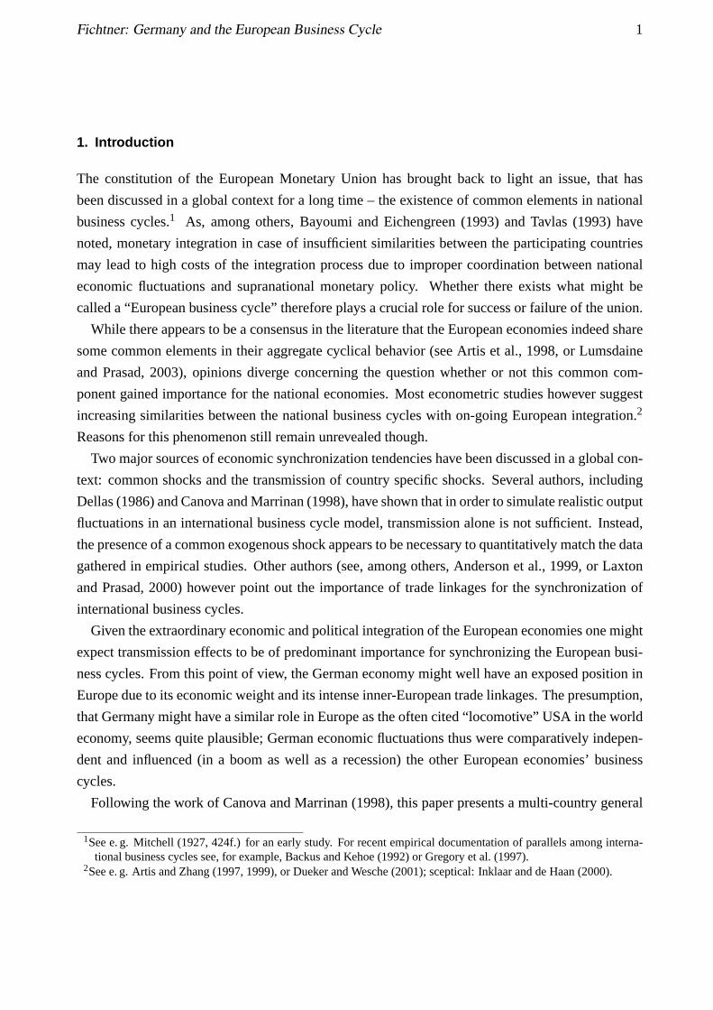
Figure 1: Impulse response functions of a 1% shock on German GDP with 95% confi-dence bands.

Austria, Germany5, France, Italy, Japan, UK and the US. Additionally included are a (highly sig-

nificant) dummy for the boom phase in Germany induced by the reunification (1991:1 until 1992:4)

and the oil price growth rate as exogenous variable. According to the usual information criteria the

lag length has been set to 1.

The impulse response functions have been simulated using the following Cholesky ordering: US,

Germany, UK, France, Italy, Austria and Japan. With the exception of Japan this ordering follows

the economic weight as indicated by the GDP in 1985 and can – given that bigger countries tend

to influence smaller countries and not vice versa – be regarded as economically quite plausible.

The exception of Japan seems justified in view of its less important economic linkages with the

European countries.

Fig. 1 plots the mean estimate of the impulse response functions to a 1% shock on German GDP

with 95% confidence bands.6 Obviously, German output shocks have significantly large and posi-

tive contemporaneous effects on the European economies, with the reaction in Austria clearly being

higher than in the other countries. As a whole, a positive interdependence between German business

cycles and those of the included European economies can be assumed.

To get an impression of changes in the relationship leading to unreliabilities in the presented re-

sults, in a next step VARs will be estimated for different subsamples. The first subsample (“70ies”)

5To avoid a jump in the data an artificial series has been created by writing back all-German values with West Germangrowth rates from 1992:1 backwards.

6Economic dependencies between Germany and Europe shall here be analyzed focusing on France, Italy and Austria,as their economic relationship to Germany has been relatively stable over the examined period and data is readilyavailable for these countries.


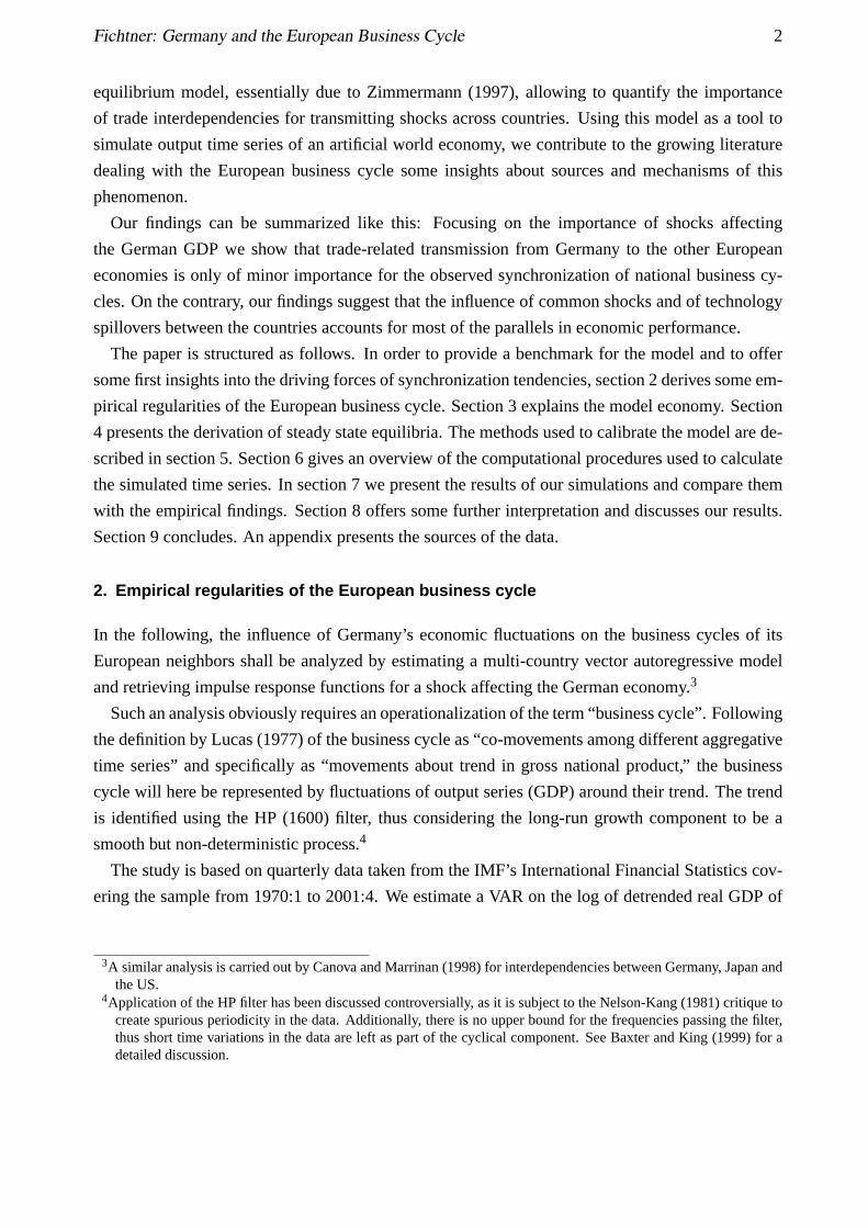
covers the period 1970:1 – 1979:4, the second subsample (“80ies”) the period 1980:1 – 1991:4,7 and

the third subsample (“90ies”) the period 1992:1 – 2001:4.

The impulse response functions for the subsamples (see fig. 2) reveal some interesting features of

the European economic system. While in the 1970ies and 1990ies positive shocks on the German

GDP have positive contemporary impacts on the other European economies, business cycle interde-

pendencies between Germany and France as well as Italy appear to be negative and relatively weak

during the 1980ies.8

This pattern of German influence on the French and the Italian business cycle seems rather un-

usual for an economic integration process that one would expect to lead to an increase in correla-

tion. Having in mind that economic synchronization might be the outcome of transmission as well

as common exogenous shocks, interpretation is straightforward though: In the 1970ies, economic

fluctuations were influenced by oil price shocks leading to a synchronization of business cycles

worldwide. By contrast, in the 1980ies such symmetric shocks were absent. Instead, business cycle

fluctuations were rather weak and marked by different economic policies: while, e. g., the French

socialist government reacted to the emerging recession in the early 1980ies with expansive fiscal

policy, a consolidation policy was implemented in Germany. Already in the early 1990ies, but still

as part of the 80ies subsample, Germany experienced an upswing after its reunification, that coin-

cided with a recession in the rest of Europe.9 During the 1990ies European economic integration

finally led to a reenforcement of economic interdependencies and thus synchronicity.

In contrast, the influence of Germany on the Austrian business cycle has remained qualitatively

unchanged over time. For all subsamples we observe a positive contemporary reaction of the Aus-

trian GDP in response to a shock leading to a deviation of the German GDP from its trend. While

the French and Italian GDP’s peak response in the 1970ies and 1990ies subsample lag for 1 quar-

ter behind the German shock (a feature not observed in the full sample analysis), Austria’s peak

response in the 80ies and 90ies arises without delay. While this might be interpreted as a sign of

the influence of common exogenous shocks on both the German and the Austrian economy, we by

no means can rule out the existence of economic linkages transmitting Germany’s economic fluc-

tuations to Austria.10 Assuming that the transmission between highly integrated economies might

be rather fast (having in mind e. g. the capital markets as a transmission channel), the use of quar-

terly data could be too coarse to allow a clear distinction between the influence of common shocks

and transmitted asymmetric shocks. On the other hand, the observed lag between Germany’s and

the French and Italian peak response can not necessarily be interpreted as an indication for the

7This upper bound is chosen in order to match the break in the data due to the German reunification.8This has been previously noted. See e. g. Seifert (1999) for an analysis of correlation coefficients in different periods.9Application of the HP filter induces additional negative correlation. As a result of the strong expansion process after

the German unification, the cyclical component of German GDP in the late 1980ies, even though following anupswing, is assessed rather low, while the other European economies experienced a boom period.

10While it seems plausible to expect the main influence to be directed from Germany to Austria, an influence fromAustria on Germany shall clearly not be precluded.


-1.0

-0.5

0.0

0.5

1.0

24

68

10

12

14

16

18

20

Re

sp

onse

of

Ge

rman G

DP

-1.0

-0.5

0.0

0.5

1.0

24

68

10

12

14

16

18

20

Re

sp

onse

of

Fre

nch G

DP

-1.0

-0.5

0.0

0.5

1.0

24

68

10

12

14

16

18

20

Re

sp

onse

of

Italia

n G

DP

-1.0

-0.5

0.0

0.5

1.0

24

68

10

12

14

16

18

20

Re

sp

onse

of

Austr

ian G

DP

-1.0

-0.5

0.0

0.5

1.0

24

68

10

12

14

16

18

20

-1.0

-0.5

0.0

0.5

1.0

24

68

10

12

14

16

18

20

-1.0

-0.5

0.0

0.5

1.0

24

68

10

12

14

16

18

20

-1.0

-0.5

0.0

0.5

1.0

24

68

10

12

14

16

18

20

-1.0

-0.5

0.0

0.5

1.0

24

68

10

12

14

16

18

20

-1.0

-0.5

0.0

0.5

1.0

24

68

10

12

14

16

18

20

-1.0

-0.5

0.0

0.5

1.0

24

68

10

12

14

16

18

20

-1.0

-0.5

0.0

0.5

1.0

24

68

10

12

14

16

18

20

80ies70ies 90ies

Fig

ure

2:Im

puls

ere

spon

sefu

nctio

nsof

a1%

shoc

kon

Ger

man

GD

Pw

ith95

%co

nfide

nce

band

s.


absence of common exogenous shocks and for high importance of transmissive effects. As Mills

and Holmes (1999, 560) note, even if countries experience a common shock, their response might

well be temporarily spread due to differing economic structures or different ways of dealing with

the shock, thus leading to an impulse response function similar to the one obtained in the case of a

transmitted idiosyncratic shock.

Therefore, the possibilities to further investigate the influence of Germany’s economic fluctua-

tions on the European business cycle on basis of the empirical findings presented above are quite

limited, as a clear distinction between the importance of transmissive effects and common shocks

for the synchronization of the national cycles is not feasible. Our analysis confirms the previously

observed strong correlation between the output fluctuations in Germany and the other economies

especially in the 1970ies and 1990ies. Evidence of reasons for this close connection remains un-

reliable though. There might be some weak indication of an increase in transmission between

Germany and France as well as Italy in the 1990ies compared to the 1970ies, as the contempora-

neous correlation decreased (thus indicating a diminished influence of common shocks), while the

lagged reaction of either country’s GDP increased. A confirmation of the hypothesis that German

economic fluctuations influence the business cycle of the other European countries by means of

transmission has yet to be given, though.

In the following sections we present an international real business cycle model, that is capable

to simulate the observed regularities of the European business cycle. By modifying the model’s

mechanisms and using the empirical findings presented above as a benchmark, we are able to assess

the importance of different driving forces of the national cycles.

3. The model

The model employed here to further investigate the influence of German business cycles on the

economic fluctuations of its European neighbors, corresponds in its characteristic features to the

basic real business cycle models presented in the seminal papers by Kydland and Prescott (1982)

and Long and Plosser (1983). Apart from rational expectations and cleared markets due to an

efficient price mechanism, this is in particular the assumption of a pure supply sided stochastic

shock (technology shock) as impulse for economic fluctuations. There is no monetary sector and

no governmental influence on the economy. The fundamental extension of this model compared

to the baseline models is the opening of the economy to international goods markets.11 In contrast

to the international models decisively developed by Backus et al. (1992) and Baxter and Crucini

(1993), heterogeneities among the countries are taken into account by Zimmermann (1997). The

following exposition is chiefly based on his work.

The model’s world economy consists of three countries differing in size and trade related vari-

11International capital markets are not explicitly modeled here. See e. g. Baxter and Crucini (1995) or Cantor and Mark(1988).


ables. The countries are populated by a constant12 number of representative agents maximizing

their lifetime utility by consuming or investing goods and varying their labor supply over time.

While goods are freely traded internationally, labor is internationally immobile.

The representative agent in countryi = 1 . . . 3 maximizes his expected lifetime utility E{Ui },

which is assumed to be representable by

Ui =

∞∑t=0

β t

γ

(ci,t

µ· (1− ni,t)

1−µ)γ, 0< β < 1,0< µ < 1, γ < 1, (1)

whereci,t is the agents consumption at timet , ni,t his working time and thus 1− ni,t his leisure,β

the discount factor, andγ the coefficient of relative risk aversion.

Each country produces one goodyi,t according to a Cobb-Douglas production function using

capitalki,t and laborni,t .13 Production is influenced by a stochastic technology parameterzi,t :

yi,t = zi,t · ki,tθni,t

1−θ , 0< θ < 1. (2)

The technology parameterzi,t follows a first order vector autoregressive process:

zt+1 =[z1,t+1 z2,t+1 z3,t+1

]T= Z + Azt + εt+1, (3)

whereεt+1 =[ε1,t+1 ε2,t+1 ε3,t+1

]T∼ N(0,V) is a vector of normally distributed serially inde-

pendent technology shocks with mean 0 and variance-covariance matrixV .14

Capital is accumulated according to

ki,t+1 = (1− δ)ki,t + xi,t , 0< δ < 1, (4)

wherexi,t is gross investment andδ the depreciation rate.

Total production of countryi , yi,t , is used domestically and abroad. Exports from countryi to

country j per capita of countryj are symbolized byyi, j,t . Thus, if the population of countryi is

given asαi :

αi yi,t = αi yi,i,t + α j yi, j,t + αkyi,k,t , i 6= j 6= k. (5)

Goods are used for consumptionci,t and investmentxi,t , where a limited substitutability between

goods of different origin is handled by introducing an Armington (1969) aggregatorG(·) into the

household’s problem. This function attaches different weightsωi, j to goods of different origin and

12As the model is used to simulate business cycles rather than growth tendencies we refrain from growth in population.13All variables are in per capita terms of the respective country.14Contemporary correlation of the technology shock in the respective countries is thus taken into account by the matrix

V and lagged correlation (e. g. due to technological spillovers) by the matrixA.


aggregates them to a single homogeneous good being consumed or invested:

ci,t + xi,t = G(yi,i,t , y j,i,t , yk,i,t) =(ωi,i yi,i,t

−ρ+ ω j,i y j,i,t

−ρ+ ωk,i yk,i,t

−ρ)− 1

ρ , (6)

with ωi,i , ω j,i , ωk,i ≥ 0, ρ ≥ 1.

4. The steady state

In the steady state the trade balances and all markets are in equilibrium. The influence of technology

shocks is set to zero (εi,t = 0). The technology parameters’ equilibrium valuez is then z =

(I − A)−1Z.

The producer’s maximization problem is

max{ki ,ni }

zi kiθni

1−θ− wi ni − (r + δ)ki , (7)

wherer is the interest rate andwi the wage. The first order conditions are then

yi = z1

1−θi

(θ

r + δ

) θ1−θ

ni , ki = θyi

r + δ, wi = (1− θ)

yi

ni, xi =

δθ yi

r + δ. (8a–d)

Households maximize their utility subject to their budget constraint:

max{ci ,ni }

1

γ

(ciµ(1− ni )

1−µ)γ, s. t.wi ni + (r + δ)ki = ci + xi . (9)

This leads to

ni =(1− θ) µ

1−µ

1+ (1− θ) µ1−µ −

δθ(r+δ)

and ci =µ

1− µ(1− θ)

yi

ni(1− ni ). (10a,b)

If pi, j or pi,k is the respective price of the foreign good valued in units of the domestic good

(price ratio, bilateral terms of trade), the household’s maximization over the three goodsyi,i , y j,i

andyk,i according to the Armington aggregator, complete markets assumed, leads to

pi, j =∂G/∂y j,i

∂G/∂yi,i=ω j,i

ωi,i

(yi,i

y j,i

)1+ρ

, (11a)

and pi,k =∂G/∂yk,i

∂G/∂yi,i=ωk,i

ωi,i

(yi,i

yk,i

)1+ρ

. (11b)

The trade balance is defined as value of exports less value of imports (expressed in prices of country


i ’s goods). Per capita of countryi , it is

tbi =α j

αiyi, j +

αk

αiyi,k − pi, j y j,i − pi,kyk,i . (12)

In the steady state, the trade balance is in equilibrium (tbi = 0) and the terms of trade are equal

to one. For the trade flows, this leads to

yi,i =yi

1+(ω j,iωi,i

) 1ρ+1+

(ωk,iωi,i

) 1ρ+1

, (13a)

y j,i =yi(

ωi,iω j,i

) 1ρ+1+ 1+

(ωk,iω j,i

) 1ρ+1

, (13b)

yk,i =yi(

ωi,iωk,i

) 1ρ+1+

(ω j,iωk,i

) 1ρ+1+ 1

. (13c)

This completes the description of the model’s steady state.

5. Calibration

As common in RBC theory, the model’s parameters are determined by calibration (see e. g. Kyd-

land and Prescott, 1996). Following Zimmermann (1997) and most of the literature the (quarterly)

interest rate in all countries is set tor = 1%. This yieldsβ = 1r+1 ≈ 0.99. The quarterly discount

rate is fixed atδ = 0.025, the capital income shareθ is set to 0.35.15 Rearranging (10a) and setting

ni = 0.3 as well asciyi= 0.75, leads toµ = 1

1+yici(1−θ)

1−nini

≈ 0.33. For the measure of risk aversion

γ = −1 is assumed.

Theωi, j are determined by settingyi,iyi

according to the average domestic production share of the

respective country’s GDP as recorded in the IMF’s International Financial Statistics.16 Additionallyy j,iyi

and yk,iyi

are set such that the countries import ratios from the two other countries match the

average import proportions as reported in the IMF’s Direction of Trade Statistics. Taking into

account, that in the long runci + xi = yi and the terms of trade in the steady state are equal to one,

one can derive the weights in the Armington aggregator asω j,i =

(y j,iyi

)1+ρ.

The calibration of the technology parameter is based on the estimation of Solow (1957) residuals.

Using time series of employment, real output and capital formation for the respective countries,

we derive a time series for the Solow residual of each country.17 As assumed in the model,zt

evolves according to a VAR(1) process. We thus use the series of the Solow residuals to estimate

15Assuming that factors are paid according to their marginal product, it follows from the production function that thehouseholds’ income share from capital equalsθ .

16Averages cover the period from 1970 to 2000. See the appendix for details.17See the appendix for sources and details of the aggregation procedure.


the parameters of this VAR process (coefficient matrixA and variance-covariance matrixV) by

ordinary least squares.

6. Synopsis of the computational procedures

As most RBC models, the model discussed in this paper can not be solved analytically due to the

functional forms of preferences and production.18 It will therefore be evaluated numerically using

a dynamic programming technique explained by Hansen and Prescott (1995) and Díaz-Giménez

(1999). This technique requires the optimization problem underlying the consumers and producers

behavior to be written in terms of a social planning problem.19 This allows us to exploit the recursive

structure of the dynamic optimization problem, as the social planner’s problem is structurally the

same in each period: given a fixed capital stockkt and technology parameterzt , he decides about

labor, consumption, investment and imports such that the expected value of the agents’ discounted

life time utility is maximized. This will be the case if the social planner maximizes a weighted sum

of the representative agents’ utility, where the weights are given by the country sizeαi .

The social planner’s optimization problem is thus given by

max3∑

i=1

αi

∞∑t=0

β t

γ

(ci,t

µ(1− ni,t)1−µ

)γ(14)

s. t. ci,t = G(yi,i,t , y j,i,t , yk,i,t

)− xi,t (15a)

αi yi,i,t = αi yi,t − α j yi, j,t − αkyi,k,t (15b)

yi,t = zi,tki,tθni,t

1−θ (15c)

zt+1 =(zi,t , z j,t , zk,t

)T= Z + Azt + εt (15d)

ki,t+1 = (1− δ) ki,t + xi,t (15e)

for all i 6= j 6= k and i, j, k ∈ {1,2,3}. Substituting (15a)–(15c) in (14) leads to the global

utility function, which serves as the social planner’s objective function in the dynamic programming

problem:

max{ni,t ,xi,t ,yi, j,t }

3∑i=1

αi

∞∑t=0

β t

γ

([G

(zi,tki,t

θn1−θi,t

−α j

αiyi, j,t −

αk

αiyi,k,t , y j,i,t , yk,i,t

)− xi,t

]µ (1− ni,t

)1−µ)γ

(16)

18Analytical solutions can be found for models with very strict assumptions, e. g. a depreciation rate of 100% andlogarithmic utility as in Long and Plosser (1983).

19According to the Second Welfare Theorem, the decentral maximization problem of consumers and producers canequivalently be analyzed in terms of a social planning problem, if there are no externalities such as distorting taxesin the considered model.


s. t. zt+1 = Z + Azt + εt , (17a)

ki,t+1 = (1− δ) ki,t + xi,t . (17b)

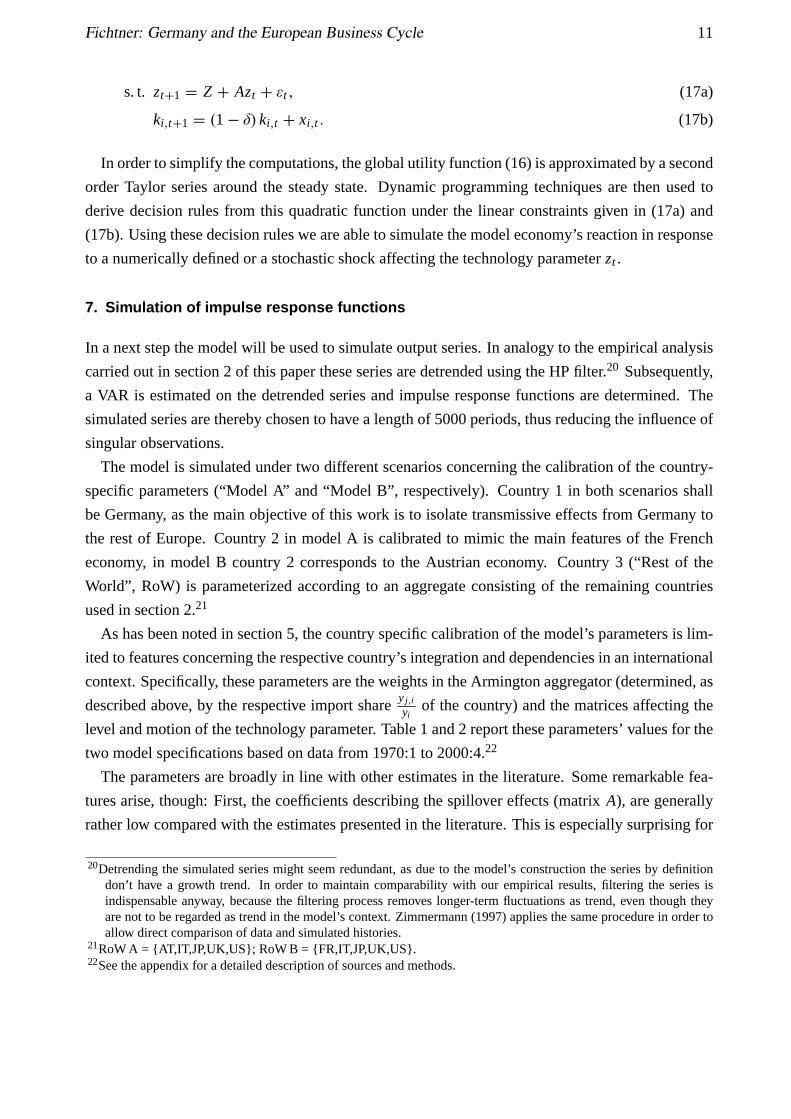
In order to simplify the computations, the global utility function (16) is approximated by a second

order Taylor series around the steady state. Dynamic programming techniques are then used to

derive decision rules from this quadratic function under the linear constraints given in (17a) and

(17b). Using these decision rules we are able to simulate the model economy’s reaction in response

to a numerically defined or a stochastic shock affecting the technology parameterzt .

7. Simulation of impulse response functions

In a next step the model will be used to simulate output series. In analogy to the empirical analysis

carried out in section 2 of this paper these series are detrended using the HP filter.20 Subsequently,

a VAR is estimated on the detrended series and impulse response functions are determined. The

simulated series are thereby chosen to have a length of 5000 periods, thus reducing the influence of

singular observations.

The model is simulated under two different scenarios concerning the calibration of the country-

specific parameters (“Model A” and “Model B”, respectively). Country 1 in both scenarios shall

be Germany, as the main objective of this work is to isolate transmissive effects from Germany to

the rest of Europe. Country 2 in model A is calibrated to mimic the main features of the French

economy, in model B country 2 corresponds to the Austrian economy. Country 3 (“Rest of the

World”, RoW) is parameterized according to an aggregate consisting of the remaining countries

used in section 2.21

As has been noted in section 5, the country specific calibration of the model’s parameters is lim-

ited to features concerning the respective country’s integration and dependencies in an international

context. Specifically, these parameters are the weights in the Armington aggregator (determined, as

described above, by the respective import sharey j,iyi

of the country) and the matrices affecting the

level and motion of the technology parameter. Table 1 and 2 report these parameters’ values for the

two model specifications based on data from 1970:1 to 2000:4.22

The parameters are broadly in line with other estimates in the literature. Some remarkable fea-

tures arise, though: First, the coefficients describing the spillover effects (matrixA), are generally

rather low compared with the estimates presented in the literature. This is especially surprising for

20Detrending the simulated series might seem redundant, as due to the model’s construction the series by definitiondon’t have a growth trend. In order to maintain comparability with our empirical results, filtering the series isindispensable anyway, because the filtering process removes longer-term fluctuations as trend, even though theyare not to be regarded as trend in the model’s context. Zimmermann (1997) applies the same procedure in order toallow direct comparison of data and simulated histories.

21RoW A = {AT,IT,JP,UK,US}; RoW B = {FR,IT,JP,UK,US}.22See the appendix for a detailed description of sources and methods.


Table 1.a: Import shares.

From:To: Germany France RoW A

Germany y1,1y1= 0.793 y1,2

y2= 0.065 y1,3

y3= 0.070

France y2,1y1= 0.048 y2,2

y2= 0.818 y2,3

y3= 0.035

RoW A y3,1y1= 0.159 y3,2

y2= 0.117 y3,3

y3= 0.895∑

1 : 1.000∑

2 : 1.000∑

3 : 1.000

Table 1.b: The technology parameter.

A =

0.881620 −0.041001 0.104630(0.03467) (0.04505) (0.06693)

−0.039868 0.943340 0.082678(0.01930) (0.02507) (0.03725)

−0.009231 −0.057053 0.917830(0.02195) (0.02852) (0.04237)

V =

2.5431E−05 5.8401E−06 1.6281E−06

5.8401E−06 7.8998E−06 1.8278E−06

1.6281E−06 1.8278E−06 1.0199E−05

Numbers in parentheses are standard errors.

Table 1: Calibration of the country specific parameters in model A.

Table 2.a: Import shares.

From:To: Germany Austria RoW B

Germany y1,1y1= 0.793 y1,2

y2= 0.187 y1,3

y3= 0.084

Austria y2,1y1= 0.047 y2,2

y2= 0.710 y2,3

y3= 0.026

RoW B y3,1y1= 0.160 y3,2

y2= 0.103 y3,3

y3= 0.890∑

1 : 1.000∑

2 : 1.000∑

3 : 1.000

Table 2.b: The technology parameter.

A =

0.856396 −0.000865 0.096106(0.04008) (0.02561) (0.06819)

0.062181 0.872364 0.104022(0.05970) (0.03814) (0.10157)

0.003042 −0.028566 0.891018(0.02494) (0.01593) (0.04243)

V =

2.6572E−05 5.6809E−06 2.2685E−06

5.6809E−06 5.8956E−05 1.8182E−06

2.2685E−06 1.8182E−06 1.0288E−05

Numbers in parentheses are standard errors.

Table 2: Calibration of the country specific parameters in model B.


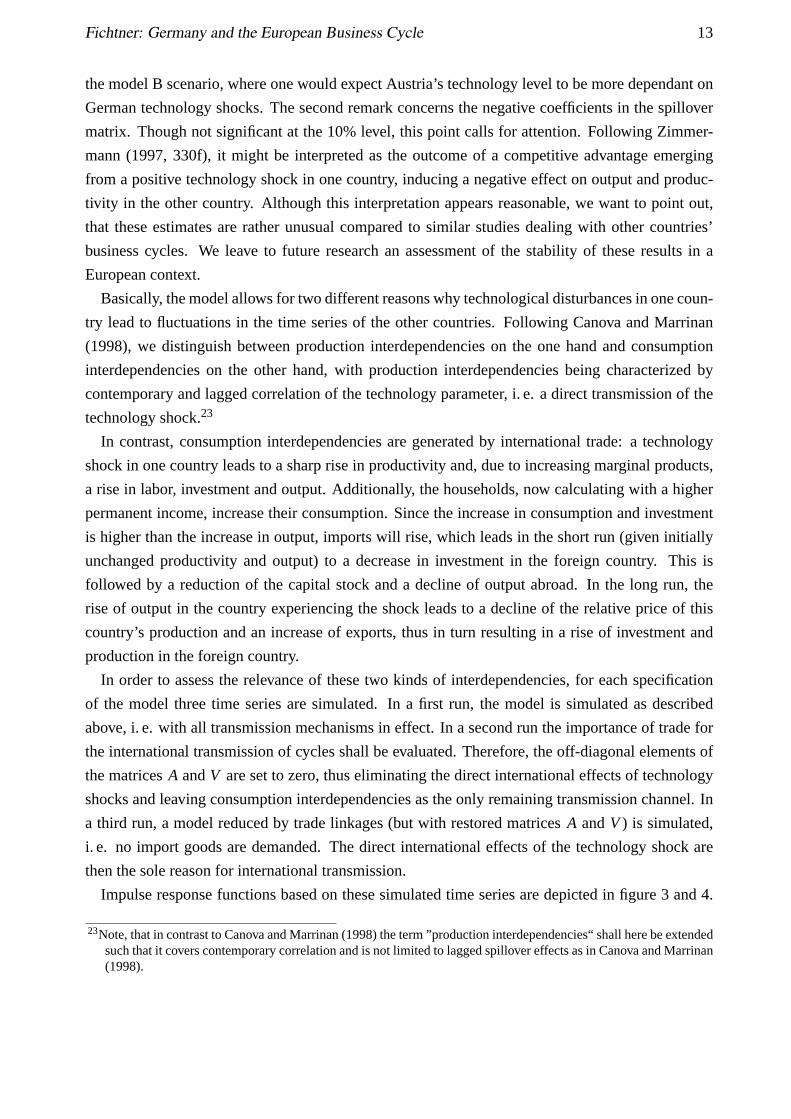
the model B scenario, where one would expect Austria’s technology level to be more dependant on

German technology shocks. The second remark concerns the negative coefficients in the spillover

matrix. Though not significant at the 10% level, this point calls for attention. Following Zimmer-

mann (1997, 330f), it might be interpreted as the outcome of a competitive advantage emerging

from a positive technology shock in one country, inducing a negative effect on output and produc-

tivity in the other country. Although this interpretation appears reasonable, we want to point out,

that these estimates are rather unusual compared to similar studies dealing with other countries’

business cycles. We leave to future research an assessment of the stability of these results in a

European context.

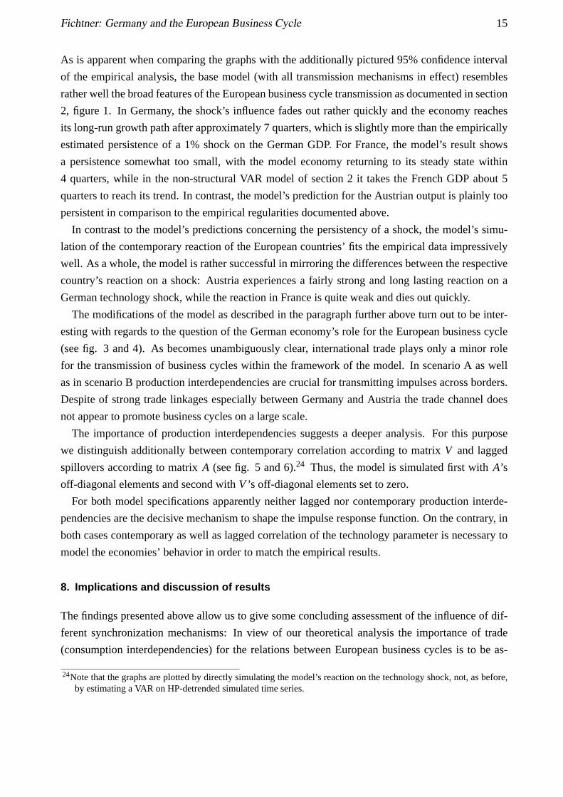
Basically, the model allows for two different reasons why technological disturbances in one coun-

try lead to fluctuations in the time series of the other countries. Following Canova and Marrinan

(1998), we distinguish between production interdependencies on the one hand and consumption

interdependencies on the other hand, with production interdependencies being characterized by

contemporary and lagged correlation of the technology parameter, i. e. a direct transmission of the

technology shock.23

In contrast, consumption interdependencies are generated by international trade: a technology

shock in one country leads to a sharp rise in productivity and, due to increasing marginal products,

a rise in labor, investment and output. Additionally, the households, now calculating with a higher

permanent income, increase their consumption. Since the increase in consumption and investment

is higher than the increase in output, imports will rise, which leads in the short run (given initially

unchanged productivity and output) to a decrease in investment in the foreign country. This is

followed by a reduction of the capital stock and a decline of output abroad. In the long run, the

rise of output in the country experiencing the shock leads to a decline of the relative price of this

country’s production and an increase of exports, thus in turn resulting in a rise of investment and

production in the foreign country.

In order to assess the relevance of these two kinds of interdependencies, for each specification

of the model three time series are simulated. In a first run, the model is simulated as described

above, i. e. with all transmission mechanisms in effect. In a second run the importance of trade for

the international transmission of cycles shall be evaluated. Therefore, the off-diagonal elements of

the matricesA andV are set to zero, thus eliminating the direct international effects of technology

shocks and leaving consumption interdependencies as the only remaining transmission channel. In

a third run, a model reduced by trade linkages (but with restored matricesA andV) is simulated,

i. e. no import goods are demanded. The direct international effects of the technology shock are

then the sole reason for international transmission.

Impulse response functions based on these simulated time series are depicted in figure 3 and 4.

23Note, that in contrast to Canova and Marrinan (1998) the term ”production interdependencies“ shall here be extendedsuch that it covers contemporary correlation and is not limited to lagged spillover effects as in Canova and Marrinan(1998).


-0.2

0.0

0.2

0.4

0.6

0.8

1.0

2 4 6 8 10 12 14 16 18 20

Full interdependencies

-0.2

0.0

0.2

0.4

0.6

0.8

1.0

2 4 6 8 10 12 14 16 18 20

Consumption interdependencies

-0.2

0.0

0.2

0.4

0.6

0.8

1.0

2 4 6 8 10 12 14 16 18 20

Production interdependencies

-.2

-.1

.0

.1

.2

.3

.4

2 4 6 8 10 12 14 16 18 20

-.2

-.1

.0

.1

.2

.3

.4

2 4 6 8 10 12 14 16 18 20

-.2

-.1

.0

.1

.2

.3

.4

2 4 6 8 10 12 14 16 18 20

Re

actio

n o

f

Ge

rma

n O

utp

ut

Re

actio

n o

f

Fre

nch

Ou

tpu

t

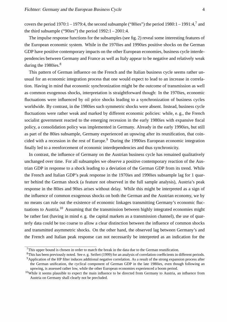
Figure 3: Simulated impulse response functions in model A: Output of the model’seconomies after a technology shock increasing German output by 1%. Depicted are thereactions with all transmission mechanisms in effect (additionally pictured are the 95%confidence bands of the empirical analysis), with pure consumption interdependenciesand with pure production interdependencies.

-0.2

0.0

0.2

0.4

0.6

0.8

1.0

2 4 6 8 10 12 14 16 18 20

Full interdependencies

-0.2

0.0

0.2

0.4

0.6

0.8

1.0

2 4 6 8 10 12 14 16 18 20

Consumption interdependencies

-0.2

0.0

0.2

0.4

0.6

0.8

1.0

2 4 6 8 10 12 14 16 18 20

Production interdependencies

-.2

-.1

.0

.1

.2

.3

.4

2 4 6 8 10 12 14 16 18 20

-.2

-.1

.0

.1

.2

.3

.4

2 4 6 8 10 12 14 16 18 20

-.2

-.1

.0

.1

.2

.3

.4

2 4 6 8 10 12 14 16 18 20

Re

actio

n o

f

Ge

rma

n O

utp

ut

Re

actio

n o

f

Au

str

ian

Ou

tpu

t

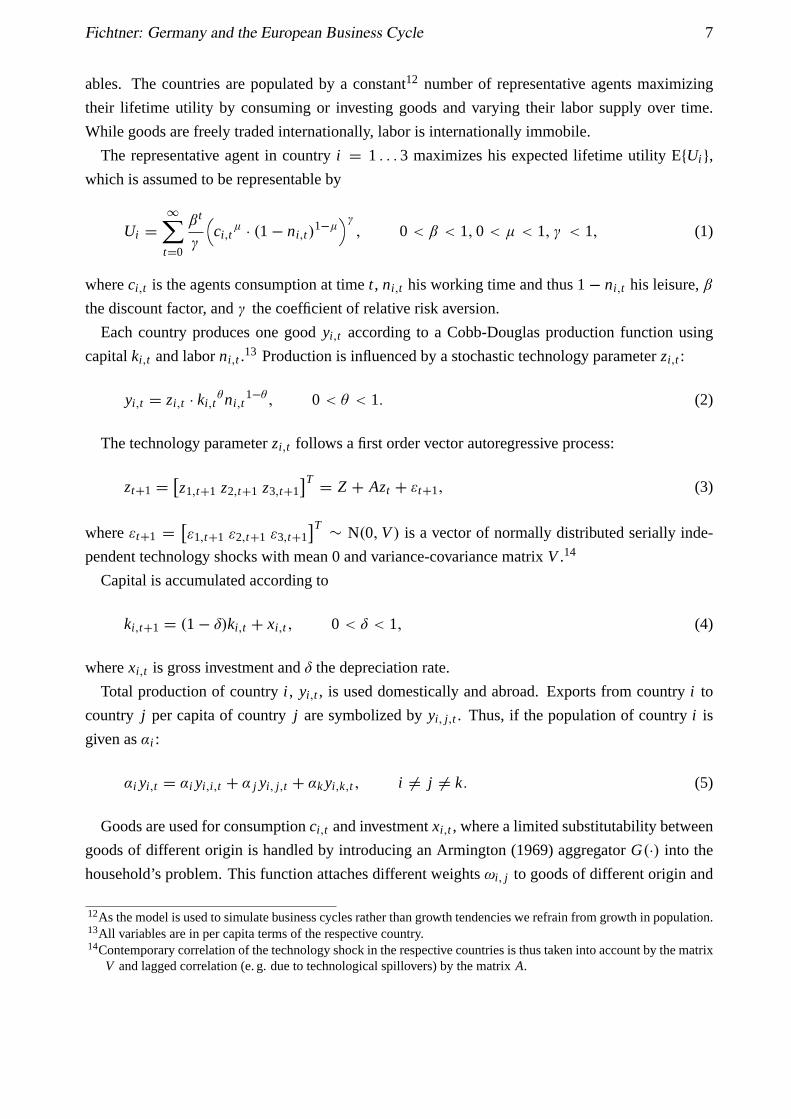
Figure 4: Simulated impulse response functions in model B: Output of the model’seconomies after a technology shock increasing German output by 1%. Depicted are thereactions with all transmission mechanisms in effect (additionally pictured are the 95%confidence bands of the empirical analysis), with pure consumption interdependenciesand with pure production interdependencies.


As is apparent when comparing the graphs with the additionally pictured 95% confidence interval

of the empirical analysis, the base model (with all transmission mechanisms in effect) resembles

rather well the broad features of the European business cycle transmission as documented in section

2, figure 1. In Germany, the shock’s influence fades out rather quickly and the economy reaches

its long-run growth path after approximately 7 quarters, which is slightly more than the empirically

estimated persistence of a 1% shock on the German GDP. For France, the model’s result shows

a persistence somewhat too small, with the model economy returning to its steady state within

4 quarters, while in the non-structural VAR model of section 2 it takes the French GDP about 5

quarters to reach its trend. In contrast, the model’s prediction for the Austrian output is plainly too

persistent in comparison to the empirical regularities documented above.

In contrast to the model’s predictions concerning the persistency of a shock, the model’s simu-

lation of the contemporary reaction of the European countries’ fits the empirical data impressively

well. As a whole, the model is rather successful in mirroring the differences between the respective

country’s reaction on a shock: Austria experiences a fairly strong and long lasting reaction on a

German technology shock, while the reaction in France is quite weak and dies out quickly.

The modifications of the model as described in the paragraph further above turn out to be inter-

esting with regards to the question of the German economy’s role for the European business cycle

(see fig. 3 and 4). As becomes unambiguously clear, international trade plays only a minor role

for the transmission of business cycles within the framework of the model. In scenario A as well

as in scenario B production interdependencies are crucial for transmitting impulses across borders.

Despite of strong trade linkages especially between Germany and Austria the trade channel does

not appear to promote business cycles on a large scale.

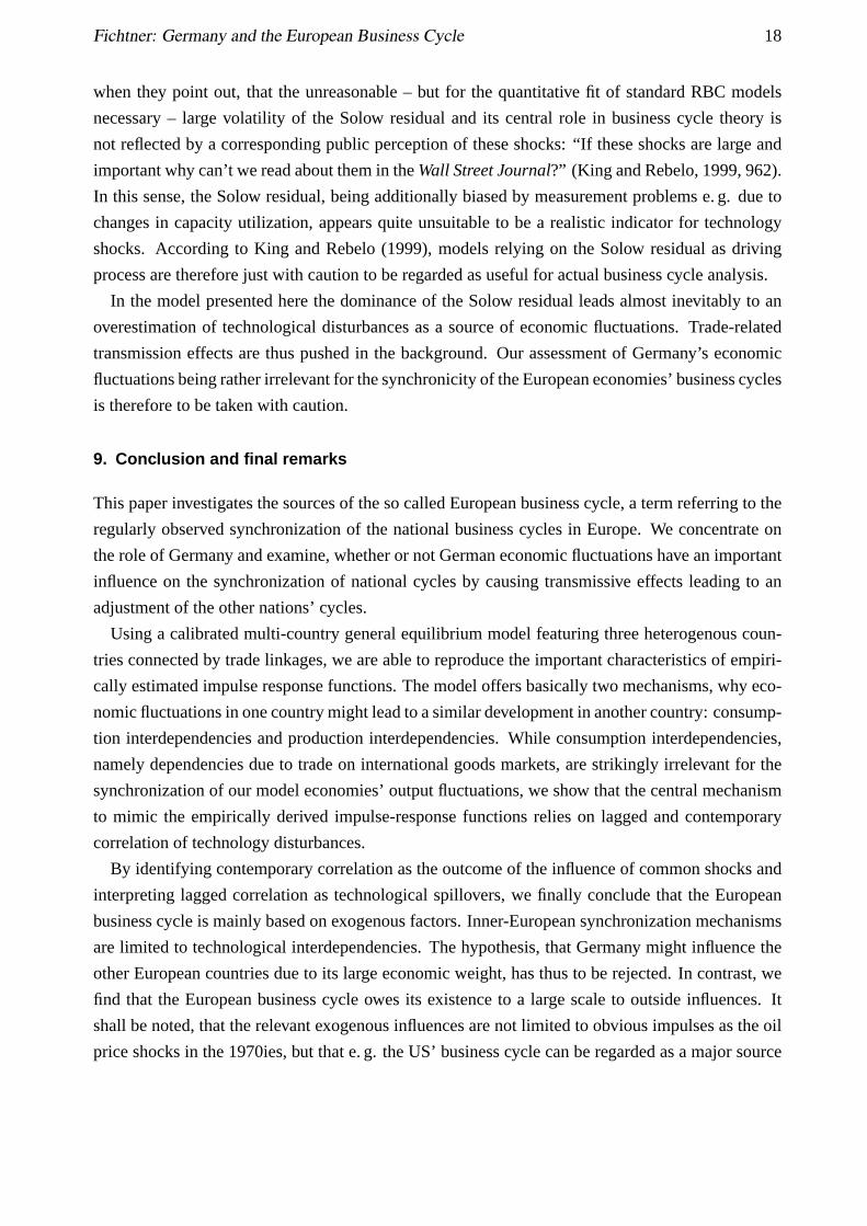
The importance of production interdependencies suggests a deeper analysis. For this purpose

we distinguish additionally between contemporary correlation according to matrixV and lagged

spillovers according to matrixA (see fig. 5 and 6).24 Thus, the model is simulated first withA’s

off-diagonal elements and second withV ’s off-diagonal elements set to zero.

For both model specifications apparently neither lagged nor contemporary production interde-

pendencies are the decisive mechanism to shape the impulse response function. On the contrary, in

both cases contemporary as well as lagged correlation of the technology parameter is necessary to

model the economies’ behavior in order to match the empirical results.

8. Implications and discussion of results

The findings presented above allow us to give some concluding assessment of the influence of dif-

ferent synchronization mechanisms: In view of our theoretical analysis the importance of trade

(consumption interdependencies) for the relations between European business cycles is to be as-

24Note that the graphs are plotted by directly simulating the model’s reaction on the technology shock, not, as before,by estimating a VAR on HP-detrended simulated time series.


-0.2

0.0

0.2

0.4

0.6

0.8

1.0

5 10 15 20 25 30 35 40 45 50-0.2

0.0

0.2

0.4

0.6

0.8

1.0

5 10 15 20 25 30 35 40 45 50-0.2

0.0

0.2

0.4

0.6

0.8

1.0

5 10 15 20 25 30 35 40 45 50

-.2

-.1

.0

.1

.2

.3

5 10 15 20 25 30 35 40 45 50-.2

-.1

.0

.1

.2

.3

5 10 15 20 25 30 35 40 45 50-.2

-.1

.0

.1

.2

.3

5 10 15 20 25 30 35 40 45 50

Reaction ofGerman GDP

Reaction ofFrench GDP

Full production interdependencies Contemporary correlation Technological spillover

Figure 5: Detailed analysis of production interdependencies in model A: Output re-sponses following a 1% shock on German GDP with full production interdependencies,with isolated contemporary correlation and lagged technological spillovers.

-0.2

0.0

0.2

0.4

0.6

0.8

1.0

5 10 15 20 25 30 35 40 45 50-0.2

0.0

0.2

0.4

0.6

0.8

1.0

5 10 15 20 25 30 35 40 45 50-0.2

0.0

0.2

0.4

0.6

0.8

1.0

5 10 15 20 25 30 35 40 45 50

-.2

-.1

.0

.1

.2

.3

.4

5 10 15 20 25 30 35 40 45 50-.2

-.1

.0

.1

.2

.3

.4

5 10 15 20 25 30 35 40 45 50-.2

-.1

.0

.1

.2

.3

.4

5 10 15 20 25 30 35 40 45 50

Reaction ofGerman GDP

Reaction ofAustrian GDP

Full production interdependencies Contemporary correlation Technological spillover

Figure 6: Detailed analysis of production interdependencies in model B: Output re-sponses following a 1% shock on German GDP with full production interdependencies,with isolated contemporary correlation and lagged technological spillovers.


sessed rather low. The role of technological interdependencies demands a more sophisticated ex-

amination. As we have shown in the preceding section, contemporary as well as lagged correlation

of the technology parameter is required in order to simulate realistic impulse response functions.

We follow Canova and Marrinan (1998, 144) in interpreting contemporary correlation as a sign

of common exogenous shocks influencing the national economies. Our results therefore imply, that

exogenous shocks are highly relevant for the existence of synchronization tendencies among the

European economies.

The interpretation of lagged correlation is not as forthright though. High off-diagonal elements

of matrix A might well be interpreted as an indication for the transmission of technology, e. g.

through the export of technically advanced intermediate goods, international knowledge transfers

or imitation of foreign goods. In this sense, the model provides some indication for an influence

of Germany’s economic developments on the other European nations’. This is not to say that this

influence necessarily points just in one direction. On the contrary, a comparison of the coefficients

of matrix A does not confirm an unidirectional effect in the case of France, where the influence ap-

pears to be relatively balanced. The existence of a “German locomotive”, that increases the foreign

productivity by technological spillovers, might be affirmed in the case of Austria, though. Still, we

can not deny the problem already discussed in section 2, that the impression of lagged correlation

might simply be induced by different economic policies to deal with a common (exogenous) shock

or by different structural conditions. This problem is as relevant for the estimation of the technology

shock’s parameters as it was relevant for the estimation of the VARs on GDPs in section 2.

Concluding, we can state that from a theoretical point of view the European business cycle is

mainly based on common exogenous shocks and mutual supply side dependencies. Given, that the

model and the chosen parameter values are a correct description of reality, the importance of trade

related transmission effects is rather low.

This result corresponds to the findings presented by Canova and Marrinan (1998) for the in-

ternational component of business cycles in Germany, Japan and the US. We can not provide an

indication for a diverging result due to the special economic situation in Europe. Neither can we

confirm the thesis of Germany having due to its size a dominant and thus synchronizing influence

on the European business cycles, nor does the deep integration of European national economies via

trade appear to have a harmonizing effect.

However, the central role of production interdependencies in the model might at least in part be

provoked by a common (and controversially discussed) characteristic of real business cycle models:

the indefiniteness of the Solow residual. The interpretation of this “measure of our ignorance”

(Abramovitz, 1956, 11) as an indicator for a country’s technology level appears inappropriate. As

notes Mankiw (1989), the observed high correlation between the Solow residual and GDP is not

necessarily to be interpreted as an indicator for the important role of technological disturbances for

business cycles, but might well have its reasons in an insufficient separation of technology shocks

from other influences when estimating the Solow residual. King and Rebelo (1999) argue similarly,


when they point out, that the unreasonable – but for the quantitative fit of standard RBC models

necessary – large volatility of the Solow residual and its central role in business cycle theory is

not reflected by a corresponding public perception of these shocks: “If these shocks are large and

important why can’t we read about them in theWall Street Journal?” (King and Rebelo, 1999, 962).

In this sense, the Solow residual, being additionally biased by measurement problems e. g. due to

changes in capacity utilization, appears quite unsuitable to be a realistic indicator for technology

shocks. According to King and Rebelo (1999), models relying on the Solow residual as driving

process are therefore just with caution to be regarded as useful for actual business cycle analysis.

In the model presented here the dominance of the Solow residual leads almost inevitably to an

overestimation of technological disturbances as a source of economic fluctuations. Trade-related

transmission effects are thus pushed in the background. Our assessment of Germany’s economic

fluctuations being rather irrelevant for the synchronicity of the European economies’ business cycles

is therefore to be taken with caution.

9. Conclusion and final remarks

This paper investigates the sources of the so called European business cycle, a term referring to the

regularly observed synchronization of the national business cycles in Europe. We concentrate on

the role of Germany and examine, whether or not German economic fluctuations have an important

influence on the synchronization of national cycles by causing transmissive effects leading to an

adjustment of the other nations’ cycles.

Using a calibrated multi-country general equilibrium model featuring three heterogenous coun-

tries connected by trade linkages, we are able to reproduce the important characteristics of empiri-

cally estimated impulse response functions. The model offers basically two mechanisms, why eco-

nomic fluctuations in one country might lead to a similar development in another country: consump-

tion interdependencies and production interdependencies. While consumption interdependencies,

namely dependencies due to trade on international goods markets, are strikingly irrelevant for the

synchronization of our model economies’ output fluctuations, we show that the central mechanism

to mimic the empirically derived impulse-response functions relies on lagged and contemporary

correlation of technology disturbances.

By identifying contemporary correlation as the outcome of the influence of common shocks and

interpreting lagged correlation as technological spillovers, we finally conclude that the European

business cycle is mainly based on exogenous factors. Inner-European synchronization mechanisms

are limited to technological interdependencies. The hypothesis, that Germany might influence the

other European countries due to its large economic weight, has thus to be rejected. In contrast, we

find that the European business cycle owes its existence to a large scale to outside influences. It

shall be noted, that the relevant exogenous influences are not limited to obvious impulses as the oil

price shocks in the 1970ies, but that e. g. the US’ business cycle can be regarded as a major source


of exogenous disturbance (Canova and Marrinan, 1998; SVR, 2001). From this point of view, an

increase in synchronization has to be attributed mainly to an approximation of policies in response

to shocks and a harmonization of structural conditions in Europe.

The model is subject to the regular criticism of real business cycle theory, though. Due to the

restriction to technology shocks as source of economic fluctuations, we allow for a limitation shed-

ding some doubt on our results. An integration of fiscal shocks in the model might improve its

reality considerably. Additionally, the high degree of abstraction rules out the possibility to simu-

late governmental actions. Appropriate modifications of the model promise interesting implications

in view of the further integration of the European economies.

Appendix

Sources of the data

The data for the GDP series presented in section 2 were taken from the IMF’s International Financial

Statistics database. We used quarterly index data at constant prices from 1970:1 to 2001:4. If

necessary, the data was seasonally adjusted using the US Census Bureau’s X12 method. For the

determination of oil price growth rates we also used the time series provided by the IMF.

The import shares (y j,i+yk,iyi

) were derived on the basis of annual IMF data from 1970 up to 2000.

We used data of real GDP and of Imports of goods and services, both in national currencies. To

determine the import and GDP figures for RoW, values were converted in US dollar and summa-

rized. We then removed internal trade according to the IMF’s Directions of Trade Statistics. From

this data, we calculated the import share and their mean value for the period [1970, 2000]. The

domestic production shareyi,iyi

is then calculated by subtracting this value from 1.

To determine the relative import sharesy j,iyi

, the import shares are split up according to IMF data.

The Directions of Trade Statistics provide the necessary figures to calculate each country’s sum of

imports to be considered in our model economy in terms of US dollar. Relating the import value

from one countryj to the total sum of imports and multiplying the resulting quota with the import

share derived above leads to the relative import sharey j,iyi

. In the case of the aggregated country

RoW we removed internal trade prior to the calculations.

The time series of the Solow residual were derived by using IMF quarterly data of real GDP from

1970:1 to 2000:4. We then multiplied each national series with a constant factor in order to match

the real GDP in international prices compiled by Heston et al. (2002) in their Penn World Tables.

We proceeded accordingly to derive the figures for the capital stock. To determine the employment

time series, OECD data was used. If available, we used the civilian employment series provided

in the Main Economic Indicators, otherwise we calculated approximate figures according to labor

force and unemployment statistics. Data for the aggregated countries were added up. Each series

has then been normalized to give it a sample mean of 1. According tozi,t =yi,t

ki,tθni,t

1−θ we calculated

time series of the technology parameter. These series have been seasonally adjusted and linearly


detrended (the model assumes a stationary technology parameter) and were then used to estimate

the matricesA andV in a VAR(1) process.

References

Abramovitz, Moses (1956): Resource and Output Trends in the United States since 1870,American Eco-nomic Review, Vol. 46, No. 2, pp. 5–23.

Anderson, Heather, Noh-Sun Kwark and Farshid Vahid (1999): Does International Trade Synchronize Busi-ness Cycles?, Monash Econometrics and Business Statistics Working Paper Series No. 8/99,http://www.buseco.monash.edu.au/Depts/EBS/Pubs/WPapers/1999/wp8-99.pd .

Armington, Paul S. (1969): A Theory of Demand for Products Distinguished by Place of Production,Inter-national Monetary Fund Staff Papers, Vol. 16, pp. 159–178.

Artis, Michael J., Hans-Martin Krolzig and Juan Toro (1998): The European Business Cycle, CEPR Dis-cussion Paper No. 2242,http://www.economics.ox.ac.uk/research/hendry/paper/AKTcepr.pdf .

Artis, Michael J. and Wenda Zhang (1997): International Business Cycles and the ERM: Is There a EuropeanBusiness Cycle?,International Journal of Finance and Economics, Vol. 2, pp. 1–16.

Artis, Michael J. and Wenda Zhang (1999): Further Evidence on the International Business Cycle and theERM: Is There a European Business Cycle?,Oxford Economic Papers, Vol. 51, pp. 120–132.

Backus, David K. and Patrick J. Kehoe (1992): International Evidence on the Historical Properties of Busi-ness Cycles,American Economic Review, Vol. 82, No. 4, pp. 864–888.

Backus, David K., Patrick J. Kehoe and Finn E. Kydland (1992): International Real Business Cycles,Journalof Political Economy, Vol. 100, No. 4, pp. 745–775.

Baxter, Marianne and Mario J. Crucini (1993): Explaining Saving–Investment Correlations,American Eco-nomic Review, Vol. 83, No. 3, pp. 416–435.

Baxter, Marianne and Mario J. Crucini (1995): Business Cycles and the Asset Structure of Foreign Trade,International Economic Review, Vol. 36, No. 4, pp. 821–854.

Baxter, Marianne and Robert G. King (1999): Measuring Business Cycles: Approximate Band-Pass Filtersfor Economic Time Series,The Review of Economics and Statistics, Vol. 81, No. 4, pp. 575–593.

Bayoumi, Tamim and Barry Eichengreen (1993): Shocking Aspects of European Monetary Integration, in:Francisco Torres and Francesco Giavazzi (Eds.),Adjustment and Growth in the European Monetary Union,Chapter 7, Cambridge: Cambridge University Press, pp. 193–229.

Canova, Fabio and Jane Marrinan (1998): Sources and Propagation of International Output Cycles: CommonShocks or Transmission?,Journal of International Economics, Vol. 46, pp. 133–166.

Cantor, Richard and Nelson C. Mark (1988): The International Transmission of Real Business Cycles,Inter-national Economic Review, Vol. 29, No. 3, pp. 493–507.

Dellas, Harris (1986): A Real Model of the World Business Cycle,Journal of International Money andFinance, Vol. 5, pp. 381–394.


Díaz-Giménez, Javier (1999): Linear Quadratic Approximation: An Introduction, in: Ramon Marimon andAndrew Scott (Eds.),Computational Methods for the Study of Economic Dynamics, Oxford, New York:Oxford University Press, pp. 13–29.

Dueker, Michael and Katrin Wesche (2001): European Business Cycles: New Indices and Analysis of theirSynchronicity, Federal Reserve Bank of St. Louis Working Paper Nr. 99-019B,http://research.stlouisfed.org/wp/1999/1999-019.pdf .

Gregory, Allan W., Allen C. Head and Jacques Raynauld (1997): Measuring World Business Cycles,Inter-national Economic Review, Vol. 38, No. 3, pp. 677–701.

Hansen, Gary D. and Edward C. Prescott (1995): Recursive Methods for Computing Equilibria of BusinessCycle Models, in: Thomas F. Cooley (Ed.),Frontiers of Business Cycle Research, Princeton: PrincetonUniversity Press, pp. 39–64.

Heston, Alan, Robert Summers and Bettina Aten (2002): Penn World Table Version 6.1, Center for Interna-tional Comparisons at the University of Pennsylvania (CICUP), October 2002.

Inklaar, Robert and Jakob de Haan (2000): Is There Really a European Business Cycle?, CESifo WorkingPaper Series No. 268.

King, Robert G. and Sergio T. Rebelo (1999): Resuscitating Real Business Cycles, in: John B. Taylor andMichael Woodford (Eds.),Handbook of Macroeconomics, Vol. 1B, Amsterdam, Lausanne, New York:Elsevier Science, pp. 927–1007.

Kydland, Finn E. and Edward C. Prescott (1982): Time to Build and Aggregate Fluctuations,Econometrica,Vol. 50, No. 6, pp. 1345–1370.

Kydland, Finn E. and Edward C. Prescott (1996): The Computational Experiment: An Econometric Tool,Journal of Economic Perspectives, Vol. 10, No. 1, pp. 69–85.

Laxton, Douglas and Eswar S. Prasad (2000): International Spillovers of Macroeconomic Shocks: A Quan-titative Exploration, IMF Working Paper No. 00/101.

Long, John B., Jr. and Charles I. Plosser (1983): Real Business Cycles,Journal of Political Economy, Vol. 91,No. 1, pp. 39–69.

Lucas, Robert E., Jr. (1977): Understanding Business Cycles, in: Karl Brunner and Allan H. Meltzer (Eds.),Stabilization of the Domestic and International Economy, Carnegie Rochester Conference Series on PublicPolicy, Vol. 5, Amsterdam, New York, Oxford: North-Holland Publishing Company, pp. 7–29.

Lumsdaine, Robin L. and Eswar S. Prasad (2003): Identifying the Common Component in InternationalEconomic Fluctuations: A New Approach,Economic Journal, Vol. 113, No. 484, pp. 101–127.

Mankiw, N. Gregory (1989): Real Business Cycles: A New Keynesian Perspective,Journal of EconomicPerspectives, Vol. 3, No. 3, pp. 79–90.

Mills, Terence C. and Mark J. Holmes (1999): Common Trends and Cycles in European Industrial Produc-tion: Exchange Rate Regimes and Economic Fluctuations,The Manchester School, Vol. 67, No. 4, pp.557–587.

Mitchell, Wesley C. (1927):Business Cycles: The Problem and Its Setting, Studies in Business Cycles No.1, New York: National Bureau of Economic Research.


Nelson, Charles R. and Heejoon Kang (1981): Spurious Periodicity in Inappropriately Detrended Time Se-ries,Econometrica, Vol. 49, No. 3, pp. 741–751.

Seifert, Michael (1999): Zum Konjunkturverbund zwischen integrierten Volkswirtschaften,Forschungsreihedes Institut für Wirtschaftsforschung Halle,Nr. 4/1999, pp. 3–36.

Solow, Robert M. (1957): Technical Change and the Aggregate Production Function,Review of Economicsand Statistics, Vol. 39, No. 3, pp. 312–320.

SVR, Sachverständigenrat zur Begutachtung der gesamtwirtschaftlichen Entwicklung (2001):Jahresgutachten 2001/02: Für Stetigkeit – Gegen Aktionismus, Stuttgart: Metzler-Poeschel.

Tavlas, George S. (1993): The ‘New’ Theory of Optimum Currency Areas,World Economy, Vol. 16, No. 6,pp. 663–685.

Zimmermann, Christian (1997): International Real Business Cycles among Heterogenous Countries,Euro-pean Economic Review, Vol. 41, No. 1, pp. 319–355.

INSTITUT FÜR WIRTSCHAFTSPOLITIK AN DER UNIVERSITÄT ZU …

Documents

Transcript of INSTITUT FÜR WIRTSCHAFTSPOLITIK AN DER UNIVERSITÄT ZU …