INSTITUT FÜR STATIK UND DYNAMIK DER LUFT- UND ... · material model was implemented in ABAQUS...
105
MASTER THESIS Abdolhamid Attaran June 2010 Modeling and Finite Element Simulation of the Viscoelastic Behavior of Dielectric Elastomers PFAFFENWALDRING 27, 70569 STUTTGART UNIVERSITÄT STUTTGART INSTITUT FÜR STATIK UND DYNAMIK DER LUFT- UND RAUMFAHRTKONSTRUKTIONEN PROFESSOR DR.-ING. BERND-H. KRÖPLIN
Transcript of INSTITUT FÜR STATIK UND DYNAMIK DER LUFT- UND ... · material model was implemented in ABAQUS...
MASTER THESIS
Abdolhamid Attaran
June 2010
Modeling and Finite Element Simulationof the Viscoelastic Behavior ofDielectric Elastomers
PFAFFENWALDRING 27, 70569 STUTTGART
UNIVERSITÄT STUTTGART
INSTITUT FÜR STATIK UND DYNAMIK DERLUFT- UND RAUMFAHRTKONSTRUKTIONENPROFESSOR DR.-ING. BERND-H. KRÖPLIN
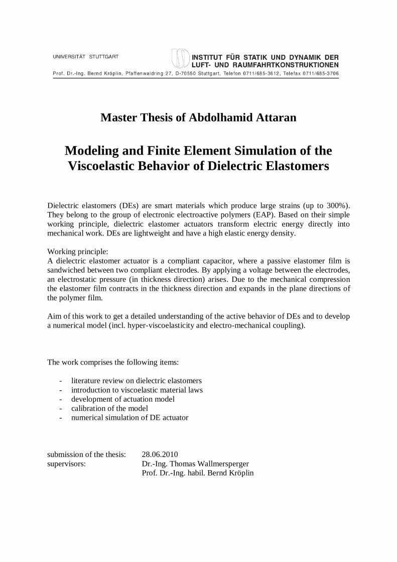
Master Thesis of Abdolhamid Attaran
Modeling and Finite Element Simulation of the
Viscoelastic Behavior of Dielectric Elastomers
Dielectric elastomers (DEs) are smart materials which produce large strains (up to 300%).
They belong to the group of electronic electroactive polymers (EAP). Based on their simple
working principle, dielectric elastomer actuators transform electric energy directly into
mechanical work. DEs are lightweight and have a high elastic energy density.
Working principle:
A dielectric elastomer actuator is a compliant capacitor, where a passive elastomer film is
sandwiched between two compliant electrodes. By applying a voltage between the electrodes,
an electrostatic pressure (in thickness direction) arises. Due to the mechanical compression
the elastomer film contracts in the thickness direction and expands in the plane directions of
the polymer film.
Aim of this work to get a detailed understanding of the active behavior of DEs and to develop
a numerical model (incl. hyper-viscoelasticity and electro-mechanical coupling).
The work comprises the following items:
- literature review on dielectric elastomers
- introduction to viscoelastic material laws
- development of actuation model
- calibration of the model
- numerical simulation of DE actuator
submission of the thesis: 28.06.2010
supervisors: Dr.-Ing. Thomas Wallmersperger
Prof. Dr.-Ing. habil. Bernd Kröplin

“We are at our very best, and we are happiest, when we are fully engaged in work
we enjoy on the journey toward the goal we’ve established for ourselves. It gives
meaning to our time off and comfort to our sleep. It makes everything else in life
so wonderful, so worthwhile.”
Earl Nightingale
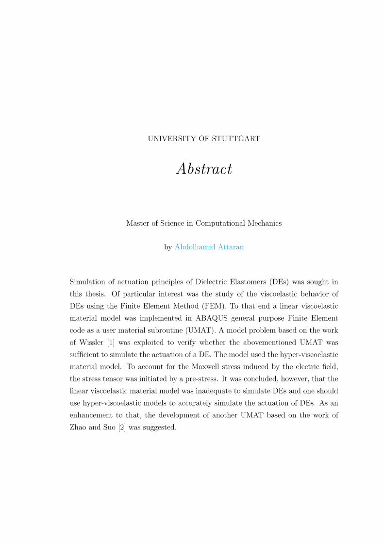
UNIVERSITY OF STUTTGART
Abstract
Master of Science in Computational Mechanics
by Abdolhamid Attaran
Simulation of actuation principles of Dielectric Elastomers (DEs) was sought in
this thesis. Of particular interest was the study of the viscoelastic behavior of
DEs using the Finite Element Method (FEM). To that end a linear viscoelastic
material model was implemented in ABAQUS general purpose Finite Element
code as a user material subroutine (UMAT). A model problem based on the work
of Wissler [1] was exploited to verify whether the abovementioned UMAT was
sufficient to simulate the actuation of a DE. The model used the hyper-viscoelastic
material model. To account for the Maxwell stress induced by the electric field,
the stress tensor was initiated by a pre-stress. It was concluded, however, that the
linear viscoelastic material model was inadequate to simulate DEs and one should
use hyper-viscoelastic models to accurately simulate the actuation of DEs. As an
enhancement to that, the development of another UMAT based on the work of
Zhao and Suo [2] was suggested.
Acknowledgements
First and foremost, I would like to express my deep and sincere gratitude to
my supervisors, Prof. Dr.-Ing. habil. Bernd Kroplin and Prof. Dr.-Ing. Thomas
Wallmersperger for giving me the opportunity to work in their research team. I
will forever be grateful for the guidance, ideas, and encouragement; their excellent
supervision has been invaluable.
I am very grateful to European Commission on Training and Education for grant-
ing me the Erasmus Mundus scholarship to study Master of Science in Computa-
tional Mechanics.
I would also like to thank the administration of the International Master of Science
in Computational Mechanics both in Barcelona and Stuttgart for the coordination
and support throughout my studies especially Prof. Dıez the coordinator of the
course, Dr. Rosato, the former coordinator of the COMMAS master program in
Stuttgart and Mrs. Zielonka, the secretary of the course in Barcelona.
Last but not least, I thank my family for supporting me in my efforts. This thesis
is dedicated to them.
iii
Contents
Abstract ii
Acknowledgements iii
List of Figures vi
List of Tables vii
Symbols viii
1 Introduction 1
1.1 General Overview . . . . . . . . . . . . . . . . . . . . . . . . . . . . 1
1.2 Structure of the Thesis . . . . . . . . . . . . . . . . . . . . . . . . . 2
2 Viscoelastic Materials 3
2.1 Fundamentals . . . . . . . . . . . . . . . . . . . . . . . . . . . . . . 3
2.2 Modeling . . . . . . . . . . . . . . . . . . . . . . . . . . . . . . . . . 5
2.2.1 General Overview . . . . . . . . . . . . . . . . . . . . . . . . 5
2.2.2 Earlier Works . . . . . . . . . . . . . . . . . . . . . . . . . . 7
2.3 Experiments . . . . . . . . . . . . . . . . . . . . . . . . . . . . . . . 14
3 Dielectric Elastomers 16
3.1 Fundamentals . . . . . . . . . . . . . . . . . . . . . . . . . . . . . . 16
3.2 Modeling . . . . . . . . . . . . . . . . . . . . . . . . . . . . . . . . . 19
3.3 Experiments . . . . . . . . . . . . . . . . . . . . . . . . . . . . . . . 24
3.4 Applications . . . . . . . . . . . . . . . . . . . . . . . . . . . . . . . 25
4 Modeling of Dielectric Elastomers 26
4.1 Introduction to Nonlinear Analysis . . . . . . . . . . . . . . . . . . 26
4.2 Nonlinear Continuum Mechanics . . . . . . . . . . . . . . . . . . . . 27
4.2.1 Continuum Body . . . . . . . . . . . . . . . . . . . . . . . . 27
4.2.2 Deformation Gradient Tensors . . . . . . . . . . . . . . . . . 28
4.2.3 Strain Tensors . . . . . . . . . . . . . . . . . . . . . . . . . . 29
iv
Contents v
4.2.4 The Concept of Stress . . . . . . . . . . . . . . . . . . . . . 30
4.3 Infinitesimal Strain Theory . . . . . . . . . . . . . . . . . . . . . . . 33
4.3.1 General Overview . . . . . . . . . . . . . . . . . . . . . . . . 33
4.3.2 Voigt-Notation . . . . . . . . . . . . . . . . . . . . . . . . . 33
4.3.3 Spherical and Deviatoric Tensors . . . . . . . . . . . . . . . 35
4.4 Balance Laws . . . . . . . . . . . . . . . . . . . . . . . . . . . . . . 35
4.5 Constitutive Equations . . . . . . . . . . . . . . . . . . . . . . . . . 38
4.5.1 General Overview . . . . . . . . . . . . . . . . . . . . . . . . 38
4.5.2 3D Formulation of the Viscoelastic Constitutive Model . . . 40
4.5.3 Constitutive Model for Dielectric Elastomers . . . . . . . . . 42
4.6 Finite Element Implementation of Linear Viscoelasticity . . . . . . 44
4.6.1 Finite Element Formulation of a Nonlinear Problem . . . . . 44
4.6.2 Stress Updates and Constant Tangent Moduli . . . . . . . . 47
4.6.3 Addition of the Maxwell Stress in the Material Model . . . . 49
4.6.4 Implementation of the Algorithm in ABAQUS . . . . . . . . 49
5 Numerical Simulation of Dielectric Elastomers 51
5.1 General overview . . . . . . . . . . . . . . . . . . . . . . . . . . . . 51
5.2 UMAT Verification . . . . . . . . . . . . . . . . . . . . . . . . . . . 51
5.3 Model Problem . . . . . . . . . . . . . . . . . . . . . . . . . . . . . 54
5.3.1 General Overview . . . . . . . . . . . . . . . . . . . . . . . . 54
5.3.2 Calibrating the Stretch Ratio . . . . . . . . . . . . . . . . . 56
5.3.3 Test Cases . . . . . . . . . . . . . . . . . . . . . . . . . . . . 56
5.3.4 Effect of Varying Applied Voltage on the Activation . . . . . 57
5.3.5 Application of UMAT . . . . . . . . . . . . . . . . . . . . . 57
5.3.6 Three Dimensional Extension . . . . . . . . . . . . . . . . . 59
6 Conclusion and Outlook 61
A User Subroutines 63
A.1 UMAT for Representation A . . . . . . . . . . . . . . . . . . . . . . 63
A.2 UMAT Developed by Prof. R. M. Hacket . . . . . . . . . . . . . . . 68
A.2.1 UMAT with Two Maxwell Elements (N = 2) . . . . . . . . . 68
A.2.2 UMAT with Four Maxwell Elements (N = 4) . . . . . . . . . 75
A.3 “SIGINI” Subroutine . . . . . . . . . . . . . . . . . . . . . . . . . . 83
Bibliography 84
List of Figures
2.1 Voigt element . . . . . . . . . . . . . . . . . . . . . . . . . . . . . . 4
2.2 Creep response . . . . . . . . . . . . . . . . . . . . . . . . . . . . . 4
2.3 Maxwell element . . . . . . . . . . . . . . . . . . . . . . . . . . . . 4
2.4 Stress relaxation . . . . . . . . . . . . . . . . . . . . . . . . . . . . 4
2.5 Wiechert element . . . . . . . . . . . . . . . . . . . . . . . . . . . . 5
3.1 DE actuator in the de-activated (left) and activated state (right) [51] 18
3.2 Different DE configurations: (a) Extenders/Bimorphs, (b) cylindri-cal actuators, (c) linear actuators, (d) inflatable membranes, (e) an-nular membranes, (f,g) planar configurations [45]. . . . . . . . . . . 18
4.1 Motion of a continuum body . . . . . . . . . . . . . . . . . . . . . . 28
4.2 Traction vector . . . . . . . . . . . . . . . . . . . . . . . . . . . . . 31
4.3 Cauchy’s stress tensor components . . . . . . . . . . . . . . . . . . 32
4.4 Material box . . . . . . . . . . . . . . . . . . . . . . . . . . . . . . . 39
4.5 Generalized Maxwell model . . . . . . . . . . . . . . . . . . . . . . 41
4.6 Out-of-plane pressure pz and lateral stress pr acting on the dielectricin a circular actuator, axisymmetric view [1] . . . . . . . . . . . . . 44
5.1 Two dimensional model problem [1] . . . . . . . . . . . . . . . . . . 54
5.2 Three dimensional model problem . . . . . . . . . . . . . . . . . . . 59
5.3 Activate DE with 3 kV . . . . . . . . . . . . . . . . . . . . . . . . . 60
vi

List of Tables
2.1 Material symmetry and the independent material constants . . . . . 7
3.1 List of the leading EAPs [5] . . . . . . . . . . . . . . . . . . . . . . 16
5.1 Material properties for UMAT verification . . . . . . . . . . . . . . 52
5.2 UMAT verification results . . . . . . . . . . . . . . . . . . . . . . . 53
5.3 DE properties from a relaxation test [48] . . . . . . . . . . . . . . . 54
5.4 Calibration results of the stretch ratio using the lateral pressureapproach . . . . . . . . . . . . . . . . . . . . . . . . . . . . . . . . . 56
5.5 Calibration results of the stretch ratio using pre-stress approach . . 56
5.6 Test cases of Maxwell Stress inclusion in the system . . . . . . . . . 57
5.7 Effect of applied voltage, U , on the elongation of DE . . . . . . . . 57
5.8 Results of DE actuation simulation with UMAT, ABAQUS Vis-coelasticity and ABAQUS Hyper-viscoelasticity . . . . . . . . . . . 58
5.9 DE material properties for UMAT . . . . . . . . . . . . . . . . . . . 58
5.10 Results of 3D DE actuation simulation . . . . . . . . . . . . . . . . 59
vii
Symbols
αi Tensor of internal variables
βi Tensor of external forces
∂Ω Surface area of the continuum body
∂ε Partial differentiation with respect to ε
∂θ Partial differentiation with respect to θ
∂I Partial differentiation with respect to I
ǫ Eigenvalue
ε Strain tensor
ε′ Isochoric (Deviatoric) strain tensor
εs Viscous strain
εp Plastic strain
ε0 Permittivity of free space
εr Dielectric constant
η Entropy per unit of mass or specific entropy
ηi Viscosity of the dashpots
θ Temperature
κ Bulk modulus
λt Stretch ratio in the thickness direction
λp Pre-stretch ratio
µ0 Instantaneous shear modulus of the spring in the
Maxwell element
viii

Symbols ix
µ∞ Long-term shear modulus of the spring in the Maxwell
element
µi Shear modulus of the spring in the Maxwell arm
ν Poisson’s ratio
ξ Reduced time
Π Functional
ρ Density
σ Cauchy (true) stress tensor
σesp Spherical stress tensor
σ′ Deviatoric stress tensor
σE Elastic stress tensor
σM Maxwell stress tensor
τ Kirchhoff stress tensor
τi Relaxation time
tr[•] Trace of a tensor
Ωt Configuration at time t (current configuration)
Ω0 Reference configuration
Ψ Helmholtz free energy per unit of mass or energy storage
function
Φ Dissipation function
ϕ Motion mapping
ϕ−1 Inverse motion mapping
B B-Matrix
b Body forces
C Constant tangent moduli
C Elasticity tensor
Cijkl The elastic coefficients
Ci i=10,20,30 Yeoh’s model coefficients

Symbols x
Dlocal The Rate of internal dissipation per unit of spatial
volume
Dcon The rate of internal dissipation by heat conduction per
unit of spatial volume
d Nodal vector
dX Material tangent vector
dx Spatial tangent vector
dL Material length
dl Spatial length
df Resultant current infinitesimal force
dS Surface element in reference configuration
ds Surface element in current configuration
df Resultant current infinitesimal Force
E Green-Lagrange strain tensor
e Euler-Almansi strain tensor
e Volumetric strain
e Internal energy per unit of mass
ei i=1,2,3 Unit vector
E Internal energy
E Young’s modulus
E Electric field
F External forces/Resultant forces acting on the material
volume
F Deformation gradient tensor
F−1 Inverse deformation gradient tensor
fint Internal forces
fext External forces
G Shear modulus
gpi Dimensionless shear modulus
Symbols xi
H Entropy
H History of internal variables/forces
I Second-order identity tensor
I Fourth-order identity tensor
I Generalized vector of internal variables
K Kinetic energy
kpi Dimensionless bulk modulus
K Tangent Stiffness matrix
M Momentum
ML Linear momentum
MO Angular momentum with respect to O
N Unit normal vector in reference configuration
N(u) Shape function
n Unit normal vector in current configuration
P First Piola-Kirchhoff (nominal) stress tensor
Pext External mechanical power
P Maxwell pressure
P Fourth-order deviatoric projection tensor
Qext External thermal power
q Spatial heat flux per unit of spatial surface area
r Residuum vector
r Distance vector
r Internal hear source rate per unit of mass
S Second Piola-Kirchhoff stress tensor
t Time
t Cauchy (true) traction vector
T First Piola-Kirchhoff (nominal) traction vector
u Displacement field (tensor)
Symbols xii
U Applied voltage
v Volume
v Velocity vector
X Position vector in reference configuration
x Position vector in current configuration
z Current Dielectric Elastomer’s thickness
z0 Initial Dielectric Elastomer’s thickness

Dedicated to my beloved parents and sister
xiii
Chapter 1
Introduction
1.1 General Overview
Dielectric Elastomers (DEs) have recently gained an unprecedented popularity to
be used as actuators replacing their own bulky traditional counterparts. One area
which benefits the most from such actuators is the field of imitating biology known
as biomimetics [3] where DEs can be served as artificial muscles. This is in part
due to DEs’ low density (ρ ≈ 900 − 1500 kg/m3) which matches that of human
muscle [4].
Dielectric Elastomer Actuators (DEAs), however, are still at their early stage of
development and there is an ever increasing demand for both experimental and
computational investigations to address the potential problems associated with
such actuators. Of particular interest is to examine efficiency, functionality, and
precision of these materials [3]. This requires the progress in such fields as re-
lated computational chemistry models, comprehensive material science, electro-
mechanics analytical tools, improved material processing techniques, viscoelastic-
ity of solids and control theory [5].
The motivation behind the present study stems itself from the growing demand
of numerical techniques to model and simulate the mechanical behavior of DEs.
Being a multifield problem, modeling and simulation of such materials is rather
complicated and only a few works are available. Of particular interest is to examine
the viscoelastic behavior of DEAs using Finite Element Method. This work is
primarily based on the findings of Goulbourne et al. [6] and Wissler [7].
1
Chapter 1. Introduction 2
The primary objective of the present study is to create the necessary tools for
modeling and simulation of the actuation principles of DEs and to create the
necessary platform for further investigations in this field. The scope of the work,
however, is limited to study the viscoelastic behavior of DEs. To that end the
constitutive equations of a viscoelastic solid will be implemented and then the
mechanical stress will be augmented by a Maxwell stress as stated by Goulbourne
et al. [6]. Study the effects of nonlinearities on the behavior of the mechanical
response is also sought through the considerations of geometrical and material
nonlinearities.
1.2 Structure of the Thesis
The first chapter is intended to present an introduction to the work followed by
objectives and scope of the work. Chapter two discusses the fundamentals of vis-
coelasticity and some modeling aspect of this subject. This chapter concludes
with a rather brief review of the works available in the literature on the subject
of viscoelasticity. Chapter three is completely devoted to the introduction of DEs
including fundamentals, modeling and the review of the existing works on mod-
eling DEs in literature. This chapter is wrapped up with some applications and
experimental aspects of DEs. The related theories are presented in chapter four
and chapter five is devoted to the results of the study followed by a discussion
on the obtained results. This thesis is concluded in chapter six including some
remarks on the possible future extension.
Chapter 2
Viscoelastic Materials
2.1 Fundamentals
In this section a basic overview of viscoelastic materials will be presented. Such ma-
terials as elastomers [8], rubbers, fibers, plastics, leathers, glasses, muscle tissues,
wood [9], and building materials such as concrete [10] exhibit a time dependent
mechanical behavior called viscoelasticity where the material response is not only
dependent on the current state of deformation but also on the whole deformation
history [11]. The present work, however, is only concerned with the viscoelastic
behavior of DEs.
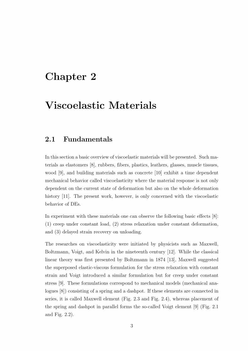
In experiment with these materials one can observe the following basic effects [8]:
(1) creep under constant load, (2) stress relaxation under constant deformation,
and (3) delayed strain recovery on unloading.
The researches on viscoelasticity were initiated by physicists such as Maxwell,
Boltzmann, Voigt, and Kelvin in the nineteenth century [12]. While the classical
linear theory was first presented by Boltzmann in 1874 [13], Maxwell suggested
the superposed elastic-viscous formulation for the stress relaxation with constant
strain and Voigt introduced a similar formulation but for creep under constant
stress [9]. These formulations correspond to mechanical models (mechanical ana-
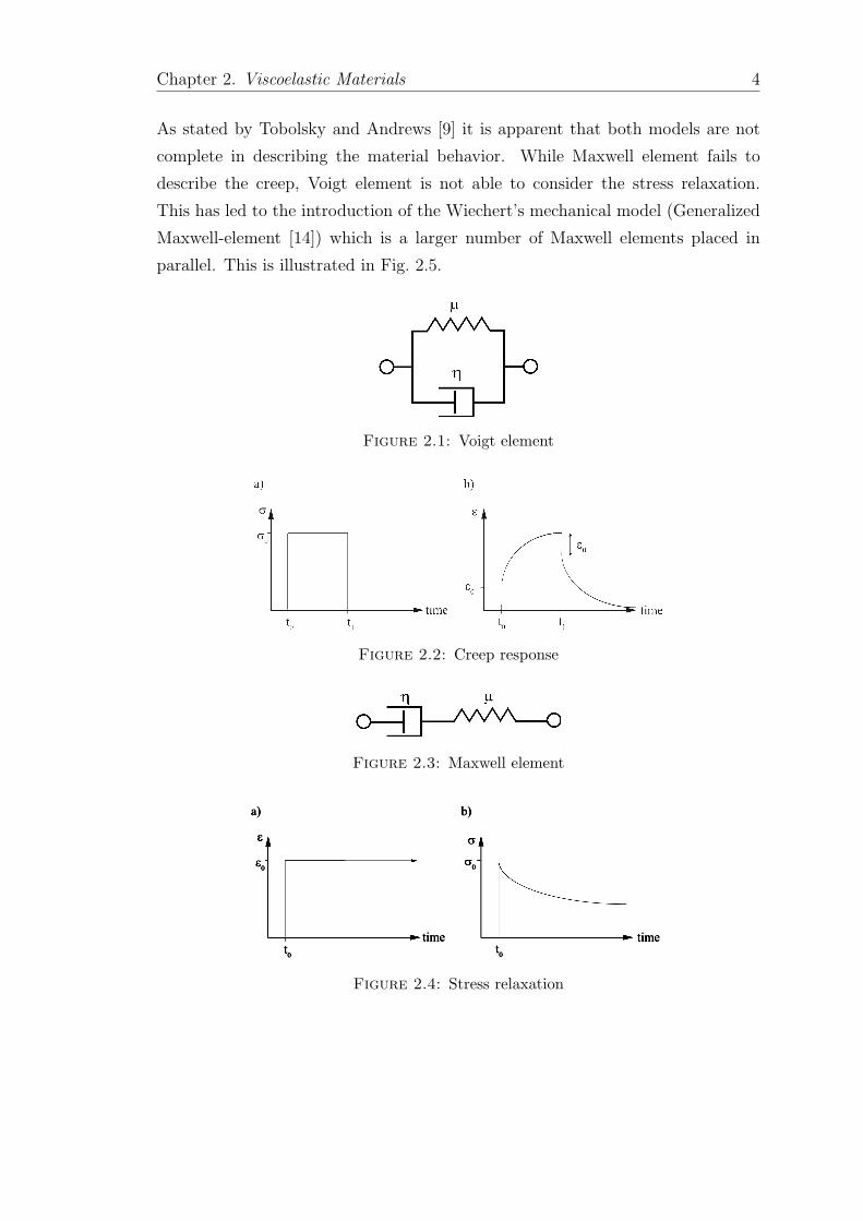
logues [8]) consisting of a spring and a dashpot. If these elements are connected in
series, it is called Maxwell element (Fig. 2.3 and Fig. 2.4), whereas placement of
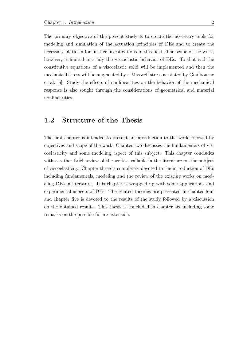
the spring and dashpot in parallel forms the so-called Voigt element [9] (Fig. 2.1
and Fig. 2.2).
3
Chapter 2. Viscoelastic Materials 4
As stated by Tobolsky and Andrews [9] it is apparent that both models are not
complete in describing the material behavior. While Maxwell element fails to
describe the creep, Voigt element is not able to consider the stress relaxation.
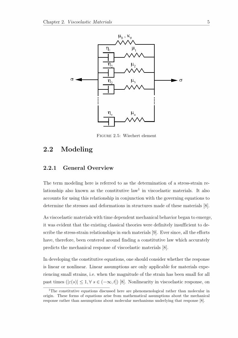
This has led to the introduction of the Wiechert’s mechanical model (Generalized
Maxwell-element [14]) which is a larger number of Maxwell elements placed in
parallel. This is illustrated in Fig. 2.5.
Figure 2.1: Voigt element
Figure 2.2: Creep response
Figure 2.3: Maxwell element
Figure 2.4: Stress relaxation
Chapter 2. Viscoelastic Materials 5
Figure 2.5: Wiechert element
2.2 Modeling
2.2.1 General Overview
The term modeling here is referred to as the determination of a stress-strain re-
lationship also known as the constitutive law1 in viscoelastic materials. It also
accounts for using this relationship in conjunction with the governing equations to
determine the stresses and deformations in structures made of these materials [8].
As viscoelastic materials with time dependent mechanical behavior began to emerge,
it was evident that the existing classical theories were definitely insufficient to de-
scribe the stress-strain relationships in such materials [9]. Ever since, all the efforts
have, therefore, been centered around finding a constitutive law which accurately
predicts the mechanical response of viscoelastic materials [8].
In developing the constitutive equations, one should consider whether the response
is linear or nonlinear. Linear assumptions are only applicable for materials expe-
riencing small strains, i.e. when the magnitude of the strain has been small for all
past times (|ε(s)| ≤ 1,∀ s ∈ (−∞, t]) [8]. Nonlinearity in viscoelastic response, on
1The constitutive equations discussed here are phenomenological rather than molecular inorigin. These forms of equations arise from mathematical assumptions about the mechanicalresponse rather than assumptions about molecular mechanisms underlying that response [8].
Chapter 2. Viscoelastic Materials 6
the other hand, occurs when there is large deformation and/or non-linear material
properties [8]; it is clear though that the linear theories are inadequate to describe
such responses of viscoelastic materials.
The derivation of linear viscoelastic constitutive equations is straightforward by
using either the consequences of linearity or mechanical analogues as stated in
the previous section (Generalized Maxwell-element) [8]. In the first approach also
known as the frequency domain approach [11], a complex structural problem in
linear viscoelasticity is solved using the correspondence principle between elas-
ticity and viscoelasticity. Based on the Laplace transformation, the viscoelastic
problem is turned into an associated elastic counterpart. After the elastic prob-
lem is solved, the solution to the original problem is obtained by performing the
numerical Laplace inverse transformation. The problem of this approach though
is that it is difficult to be extended to nonlinear problems.
In the second approach also known as the time domain approach [11], by the
virtue of the incremental finite element method, the incremental equations are
formulated, and the problem is eventually solved step-by-step. Because a recursive
form of constitutive equations is used, this approach saves much computer storage,
as compared with the Laplace inverse transformation and can easily be extended
to nonlinear problems.
There is, on the other hand, no generally accepted well-defined form for the con-
stitutive equations for nonlinear viscoelastic solids [8]. Nonetheless there are some
theories which can be used to establish the constitutive laws for nonlinear vis-
coelastic solids; among others are, rate and differential type constitutive equations,
Green-Rivlin multiple integral constitutive equation, finite linear viscoelasticity,
Pipkin-Rogers constitutive theory, quasi-linear viscoelasticity, and K-BKZ consti-
tutive theory 2 [8].
Other considerations in determination of the constitutive equations are the ma-
terial symmetry restrictions and compressibility of the materials [8]. Assuming
to be incompressible, material symmetry restriction means whether the material
is isotropic, transversely isotropic, orthotropic, or fully anisotropic. In a fully
anisotropic case, there are 21 independent material constants in the elasticity ten-
sor. This number reduces to 9 for orthotropic materials while there are only 5
independent constants in the case of transversely isotropic materials. An isotropic
2Proposed by Kaye [15], Bernstein, Kearsley, and Zapas [16]
Chapter 2. Viscoelastic Materials 7
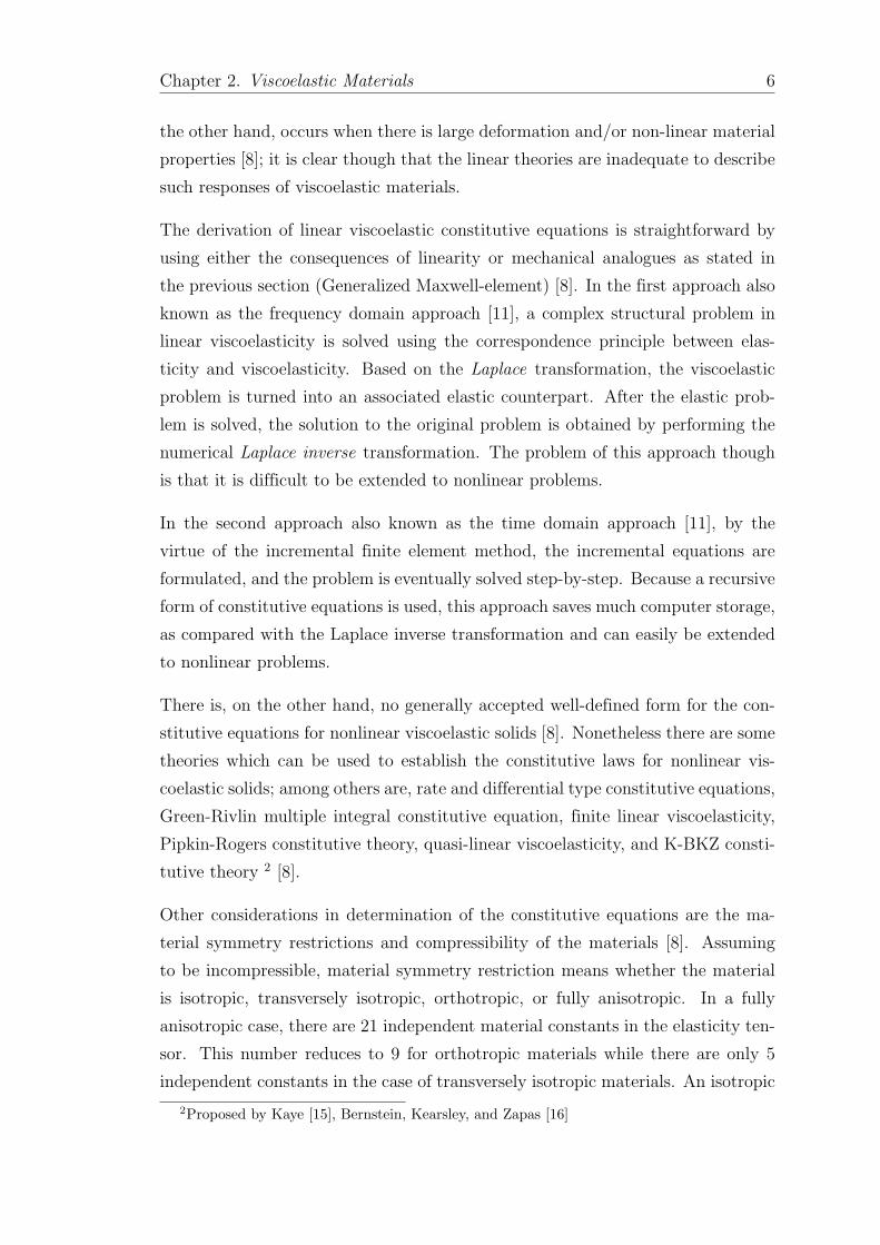
material has only 2 independent material constants. This has been summarized
in Table 2.1.
Table 2.1: Material symmetry and the independent material constants
Material Symmetry Independent Material Constants
Fully Anisotropyic Materials Ex, Ey, Ez;νx, νy, νz, ν⊥xy, ν⊥xz, ν⊥yz, ν‖xy, ν‖xz, ν‖yz;Gx, Gy, Gz, G⊥xy, G⊥xz, G⊥yz, G‖xy, G‖xz, G‖yz
Total number: 21
Orthotropic Materials Ex, Ey, Ez;νxy, νxz, νyz;Gxy, Gxz, Gyz
Total number: 9
Transversely Isotropic Materials Ex, Ez, νx, νz, Gxz
Total number: 5
Isotropic Materials E & ν
Total number: 2
In the following some earlier works on modeling the viscoelastic materials are
briefly reviewed.
2.2.2 Earlier Works
One of the earliest studies on modeling viscoelastic behavior of materials traces
back to 1945 when Tobolsky and Andrews [9] exploited a molecular approach to
describe the mechanical behavior of materials for which the classical theories of
solid mechanics and fluid mechanics were insufficient. Their attention was mainly
given to the rubberlike materials. They performed series of creep and relaxation
tests to validate their theoretical approach. Through these experiments they ob-
served three regions of stress-temperature-time dependence; namely, a low, an
intermediate and a high temperature region and discussed the creep and relax-
ation mechanism in each of these regions from a molecular point of view.
Later on, Read [17] presented his method of stress analysis for compressible vis-
coelastic materials in 1950. In his approach he used Fourier integral and operator
methods to demonstrate that elasticity theory could be further extended to ac-
count for time-dependent mechanical behavior of isotropic materials. According
to him his method was easily extendible to the fully anisotropic case.
In 1956, Lee [18] published a paper which was mainly concerned with the stress
analysis of linear viscoelastic materials such as polymers and plastics. In this paper
Chapter 2. Viscoelastic Materials 8
he talked about three major problems in developing any method of stress analysis;
namely, (1) finding the properties of material, (2) deciding on the suitable model
or operator, and (3) analyzing the stress distribution. He adopted the quasi-static
method for his work although he finally argued that there were some limitations
associated with this method.
Motivated by the challenging mathematical problems and the increasing use of in-
elastic materials, Lee [19] proposed another method of stress analysis of viscoelastic
materials. He used the operator relations to represent a given viscoelastic body
just two years after he published his paper on stress analysis of linear viscoelastic
materials [18]. He asserted that either differential or integral operator relation be-
tween stress and strain was more convenient, whereas the integral operators were
more convenient for relaxation and creep functions.
In line with the development in nonlinear continuum mechanics in early 1960s,
Coleman and Noll [20] proposed the fundamental assumptions of linear viscoelas-
ticity. They first presented the theory of infinitesimal viscoelasticity based on the
assumption that at microscopic level the substances could be regarded as spring
and dashpots connected in a complex network. This assumption could make the
formulation of the theory simple since it considered the smoothness at macroscopic
level. To characterize the smoothness they introduced the history of deformation,
and to measure the level of smoothness they defined a norm indicating how two
histories were close to each other. Further in their work, by the help of the theory
of nonlinear continuum mechanics they presented the theory of finite linear vis-
coelasticity and treated the classical infinitesimal viscoelasticity as a special case.
They contented, however, that these two theories had one fundamental difference;
the infinitesimal theory was not physically meaningful since it did not include the
basic ingredients required for material objectivity; i.e. invariants. Conversely the
finite linear theory contained these basic ingredients, hence could be used for finite
deformations.
Meanwhile, Pipkin [21] suggested some nonlinear integrals and argued that un-
der proper assumptions, the approximation of these integrals provided the basic
constitutive law for small deformations of viscoelastic solids. To that end he con-
sidered conditions where the deformation was small but finite for materials with
memory. Based on the work of other researchers (Green and Rivlin [22]; Noll [23]),
he reviewed the derivation of these nonlinear integrals which were relating stress
Chapter 2. Viscoelastic Materials 9
and strain. He also asserted that the assumption of isotropy or incompressibility
made these integral relatively simple.
In 1968, Zienkiewicz and co-workers [24], developed a general numerical proce-
dure to solve a broad-class of viscoelastic problems of the quasi-static type. Their
research was mainly concerned with the creep analysis in the field of concrete tech-
nology and rock mechanics. In their work, they demonstrated how to extend such
numerical methods as the finite element method applicable to elastic problems
to account for viscoelasticity. They exploited Kelvin-Voigt elements to represent
the material behavior. They asserted that this method was suitable for compu-
tational purposes. Next, they validated their approach against the exact solution
of viscoelasticity and tested the rate of convergence of their methods of solution.
They finally argued that the main obstacle of the future research would be the
insufficient physical data regarding the material behavior.
Two years later, Taylor et al. [25] proposed a numerical procedure to solve linear
viscoelasticity problems where thermal effects were also included. This algorithm
stemmed from a finite element discretization to a set of simultaneous linear integral
equations. They asserted that exclusion of the temperature history would result in
a set of Volterra integral equations which could be treated using integral transform
method, while by the inclusion of temperature history these equations were solved
using a step-forward integral procedure. Being computationally inefficient, they
adopted an alternative scheme to solve the latter case where the kernel functions
of the integral equations were presented by this series:
K(ξ − ξ′) =I∑
i=1
Ki fi(ξ) gi (ξ′) (2.1)
where ξ is the reduced time, ξ′ = ξ(t′), and fi and gi were the elements of the a
complete set.
To conclude their work, Taylor and co-workers investigated the validity of their
proposed algorithm by applying it to a thermal plane-stress analysis of a thin-
walled cylinder.
In the meantime, Pipkin and Rogers [26] suggested an integral series representation
of nonlinear viscoelasticity. Prior to their work most of the researches were based
on the multiple integral representation suggested by Green and Rivlin in 1957.
They contended, however, that this kind of representation posed such problems
Chapter 2. Viscoelastic Materials 10
as (1) the difficulty of stress and deformation analysis, (2) major experimental
difficulty, and (3) possessing no inherent meaning independent of the choice of
strain measure, when there was a strongly nonlinear viscoelastic response. Their
model was believed to solve or improve the aforementioned problems. In order to
consider strong nonlinearity as simple as possible, the first term in their integral
series representation was a single integral with a nonlinear integrand. In addi-
tion, they arranged the series in such a fashion that the experimental data could
be used directly. This was to make the experimental determination of material
characteristics simpler.
Schapery [27] proposed a three-dimensional nonlinear constitutive model which
was in particular consistent with the nonlinear responses of some metals and plas-
tics in 1969. To that end he discussed certain methods of characterizing nonlinear
viscoelastic solids, i.e. developing constitutive relations based on the thermody-
namic principles, and using experimental data as an assessment tool for the mate-
rial properties. The experiment consisted of uniaxial loading under fixed environ-
mental conditions and the influence of the factors such as temperature, humidity,
and aging.
Partom and Schanin [28] presented a nonlinear viscoelastic model based on the
general Maxwell model with linear springs and nonlinear dashpots. Despite the
two already existing integral representations of nonlinear viscoelasticity (multiple
and single integral representations), their approach was based on the evolution of
the stresses as the internal state variables. They applied this approach to predict
the response of various uniaxial loadings and the creep problem of a clamped beam.
Using the obtained results, they validated the model. They finally suggested this
procedure was simple and straightforward.
One year later, in 1984, Keren et al. [29] developed a two dimensional axisymmetric
finite difference code based on the nonlinear viscoelastic procedure developed in
Ref. [28]. Their test case was a thin disc glued between two rigid metal anvils
loaded in axial direction. With this test case they demonstrated that it was
impossible to correctly predict the response of the specimen with linear viscoelastic
model.
Another approach to nonlinear viscoelasticity was depicted by Rendell et al. [30]
in 1987 based on the “coupling model” of relaxation. Coupling model, as they
explained, had the proven potential to relate the features observed in nonlinear
Chapter 2. Viscoelastic Materials 11
viscoelastic experiment to molecular motions. Giving a brief review of the previous
works in the field, they asserted that the nonlinear viscoelasticity models for glassy
polymers should meet the following requirements:
1. to be dependent on stress or strain history,
2. to have a constitutive equation non-separable in stress or stress and time,
3. to have a physical meaning for all the parameters,
4. to allow for assessment of material structure toward equilibrium,
5. to predict σ(t) and ε(t) for a variety of stress and strain histories,
6. to predict the dependencies on all physical variables,
7. and to be consistent with the linear models.
They concluded that the simulations using this model revealed many of the im-
portant features. These features were also observed experimentally for various
strain histories. As an extension of their work, they suggested the inclusion of
more complicated conditions such as fatigue and multiaxial experiments.
Gramoll et al. [31] developed a numerical procedure to solve nonlinear viscoelastic
problems of orthotropic materials such as fiber-reinforced plastics (FRP) lami-
nated composites. Exhibiting strong time-dependency, the classical lamination
theory also known as CLT was clearly not sufficient to accurately predict the evo-
lution of strains and stresses over the time. Making use of the modified Kelvin
elements, they included the nonlinearity in the model. They exploited an implicit
solution scheme to solve the differential equations that modeled each of the Kelvin
elements. They finally used the Newton-Raphson method to solve the resulted si-
multaneous nonlinear equations. This choice of solution schemes, therefore, led
to an unconditionally stable numerical procedure. Gramoll and co-workers later
calibrated their predictions using their proposed method with a number of actual
experimental tests.
In the beginning of the 1990s, Krishnaswamy et al. [32] presented a finite element
algorithm being able to describe both linear and nonlinear viscoelastic material
response. In particular, they intended to examine the deformation and failure
behavior of such materials. According to them this algorithm was suitable for
Chapter 2. Viscoelastic Materials 12
analyzing the time-dependent behavior of cracks in viscoelastic materials. They
contended the differential representation was much easier to include the nonlinear
effects in the formulation of viscoelastic material model. As such, they exploited
the differential representation of viscoelastic materials instead of the integral rep-
resentation in the development of this algorithm. Having verified their algorithm
for the case of a uniaxial tensile specimen and an infinite plate with a hole sub-
jected to a remote uniaxial stress, Krishnaswamy and co-workers, then, used this
algorithm for stress and strain field determination near the crack tip of a moving
crack tip.
Motivated by the increasing application of polymers in engineering, Losi and
Knauss [33] addressed the problem of transient and residual stresses in struc-
tural parts in a paper published in 1992. This problem was due to the formation
of such structural parts at high temperature and cooling below the glass tran-
sition temperature. This in conjunction with the associated heat flow and in-
homogeneous temperature fields led to the development of residual stress. They
discussed the aforementioned problem from a thermorheological point of view and
examined their proposed methodology using an infinite cylinder and in a sphere
for three constitutive models with different accuracy; namely, the “elementary”
model, the “thermorheological” model, and the “semi-elementary” model. They,
finally demonstrated that using their procedure, the residual stresses could be
higher than an elastic analysis and, thus, the “stress-free temperature” was found
to be dramatically above the glass transition.
Ghazlan et al. [34], on the other hand, developed a complete general formulation of
linear viscoelastic creep model. This model could easily be extended to deal with
such complex viscoelastic problems as aging materials, thermoviscoelastic and dy-
namic analysis. The primary objective of their proposed model was tackling the
computer storage problem of the stress history. To this end they based their model
on a discrete creep spectrum3 and an incremental constitutive equation. Deriving
the finite element formulation of the governing equations from the principle of
virtual displacements, they demonstrated the functionality of their proposed nu-
merical procedure through a plan-stress plate, a steady-state harmonic oscillation,
a circular cylindrical shell, and a spherical shell.
Zaoutsos et al. [35] proposed a material model describing the nonlinear viscoelas-
tic response of unidirectional carbon-fiber-reinforced polymer (FRP) composites.
3A finite serries of Kelvin elements coupled with an elastic and viscous response [34].
Chapter 2. Viscoelastic Materials 13
They modified the Schapery’s nonlinear viscoelastic model by adding a viscoplas-
tic term, and determined the nonlinear viscoelastic parameters using a new data-
reduction method. These nonlinear parameters were introduced in the creep/re-
covery of FRP. Zaoutsos and co-workers, finally, validated their proposed method
through an experiment.
At the same time, Kaliske and Rothert [14] suggested a linear viscoelastic ap-
proach at small and finite strains. They presented the mixed finite element for-
mulation of their proposed numerical procedure for time-dependent deformations
of rubber-like structures. They, additionally, discussed such experimental aspects
of viscoelasticity as time-temperature superposition principle, WLF-equation, and
master curves along the parameter identification in viscoelastic problems.
Motivated by the short coming in addressing the general problem of full thermo-
mechanical coupling, large deformation and larger deviations away from thermo-
dynamic equilibrium in earlier researches, Reese and Govindjee [36] proposed a
model for finite thermo-viscoelasticity in 1998. According to them this model was
physically reasonable and numerically tractable. They asserted, however, that
this model yielded results which were more qualitative than quantitative due to
the lack of thermo-mechanical coupling experimental results. The development of
their numerical procedure was based on the assumptions of (1) multiplicative split
of deformation gradient into elastic and inelastic parts, and (2) additive split of
Helmholtz free energy into equilibrium and non-equilibrium parts.
Deriving the constitutive relations utilizing the Clausius-Duhem inequality, Reese
and Govindjee used an efficient predictor-corrector algorithm to integrate the evo-
lution equation of the constitutive relations and solved the respective initial bound-
ary value problem using a nonlinear finite element method. They, ultimately, ap-
plied their procedure to examples of a shear test, and bearing, to demonstrate
“physically interesting thermo-mechanical coupling effects” and to prove the ro-
bustness of their finite element formulation. They, however, emphasized the need
for more efficient solution techniques for three dimensional cases and suggested
such techniques as indirect solvers or domain decomposition.
Circular areas like notches and cracks where stress concentrations were likely to
happen, as well as the existence of a process (failure) zone around the crack tip are
among the sources of nonlinearities in structures made of polymers [37]. By virtue
to this fact, Masuero and Creus [37], proposed a finite element algorithm based on
Chapter 2. Viscoelastic Materials 14
Schapery’s nonlinear viscoelastic formulation for fractures and verified their sug-
gested algorithm through three cases of uniaxial tensile specimen, hollow cylinder
under internal pressure, and hollow cylinder with radial temperature distribution
under pressure. They also discussed the possibility of modeling improvement by
introduction of nonlinearity in the process zone through a damage mechanism.
Recently Drapaca et al. [38] and Wineman [8] published two separate review papers
discussing the nonlinear constitutive laws in nonlinear viscoelasticity. Presenting
a complete overview of the linear constitutive equations, Drapaca et al. were
aimed at providing a review of the classical representation of constitutive laws for
nonlinear viscoelastic materials and a unified continuum mechanics formulation.
Wineman, on the other hand, intended to review all the aspects of modeling in
viscoelastic material from a phenomenological point of view. Starting from some
historical perspective and presenting the derivation of constitutive equations for
linear viscoelasticity using different approaches, Wineman concluded that there
was no generally accepted well-defined form for the constitutive equations for
nonlinear solids as there was for linear viscoelastic solids. He, however, included
some the more well-known nonlinear constitutive equations such as Green-Rivlin
multiple integral constitutive equations, finite linear viscoelasticity, Pipkin-Rogers
constitutive theory, etc.
2.3 Experiments
In this section a very brief overview on experimental procedure is presented. This
section is by no means complete and interested readers are referred to the classical
texts on viscoelastic materials such as [39] for a comprehensive overview of the
subject matter.
Experimental procedures for viscoelastic materials are similar to experimental pro-
cedures in any other branches of mechanics and include load application, mea-
suring, strain and displacement, and transient behavior identification [39]. As
explained in Sec. 2.1 while performing such procedures one can observe such phe-
nomena as creep, stress relaxation, and delayed strain recovery on unloading. In
the following the first two phenomena are elaborated in more details.
Creep experiments as the simplest method in experimental viscoelasticity is
carried out by applying constant stress using deadweight over a sufficiently long
Chapter 2. Viscoelastic Materials 15
period of time and at elevated temperature [39]. The material responds to the
stress with a strain that increases until failure [40]. Viscoelastic creep data can be
presented by plotting the creep modulus (constant applied stress divided by the
total strain at a particular time) as a function of time. The creep response of a
viscoelastic material is illustrated in Fig. 2.2 [41]. Slope of the creep curve at any
point is called creep rate. If the specimen under the test is not failed the creep
recovery may be measured [42].
Stress relaxation test, on the other hand, is based on the relief of stress under
constant strain [42]. Such test is performed on a deformed specimen and the
decrease in stress is recorded over a prolonged period of time and at constant
elevated temperature. In this case the stress is plotted as a function of time as
portrayed in Fig. 2.4.
Chapter 3
Dielectric Elastomers
3.1 Fundamentals
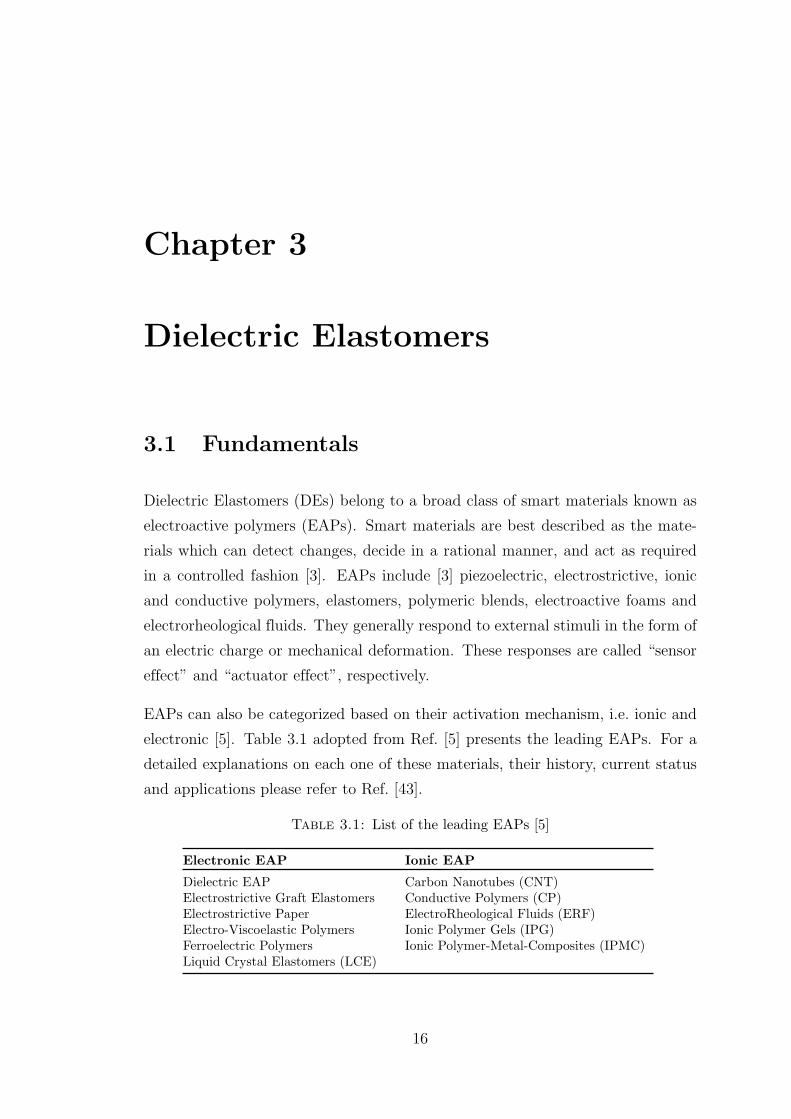
Dielectric Elastomers (DEs) belong to a broad class of smart materials known as
electroactive polymers (EAPs). Smart materials are best described as the mate-
rials which can detect changes, decide in a rational manner, and act as required
in a controlled fashion [3]. EAPs include [3] piezoelectric, electrostrictive, ionic
and conductive polymers, elastomers, polymeric blends, electroactive foams and
electrorheological fluids. They generally respond to external stimuli in the form of
an electric charge or mechanical deformation. These responses are called “sensor
effect” and “actuator effect”, respectively.
EAPs can also be categorized based on their activation mechanism, i.e. ionic and
electronic [5]. Table 3.1 adopted from Ref. [5] presents the leading EAPs. For a
detailed explanations on each one of these materials, their history, current status
and applications please refer to Ref. [43].
Table 3.1: List of the leading EAPs [5]
Electronic EAP Ionic EAP
Dielectric EAP Carbon Nanotubes (CNT)Electrostrictive Graft Elastomers Conductive Polymers (CP)Electrostrictive Paper ElectroRheological Fluids (ERF)Electro-Viscoelastic Polymers Ionic Polymer Gels (IPG)Ferroelectric Polymers Ionic Polymer-Metal-Composites (IPMC)Liquid Crystal Elastomers (LCE)
16
Chapter 3. Dielectric Elastomers 17
Operating under the so-called “dry operation” condition, Electronic EAPs can
easily be commercialized and their simple fabrication process and longer lifetime
is guaranteed [44]. They, however, require a higher actuation voltage than ionic
EAPs of about 2 kV [45].
Used as the base material in the present study, DEs are electronic EAPs which
deform extensively in the presence of an electric field and can hence be used as
actuators in adaptive structures. DEs are capable of about 100% deformation
upon activation [45]. The most common DEs are Acrylic elastomers (e.g. 3M
VHB series) and silicone (e.g. Nusil R31-2186 or CF 19-2186; Dow Corning HS
III RTV) [46, 47]. Example of applications of DEs as actuators include [3, 46–
48]: micro air vehicle, flat panel loudspeakers, video displays, haptic devices,
disk drivers, mobile mini- and micro-robot, micropumps and microvalves. For a
more complete list of applications please refer to the review paper of Biddiss and
Chau [46].
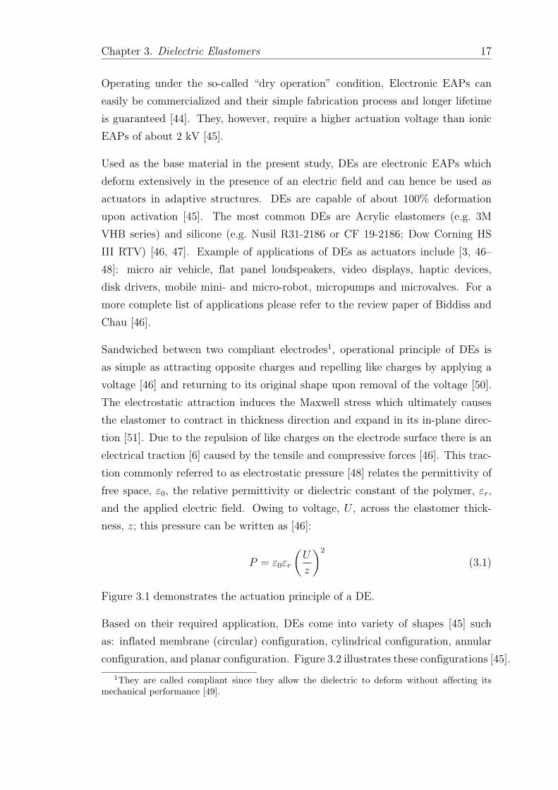
Sandwiched between two compliant electrodes1, operational principle of DEs is
as simple as attracting opposite charges and repelling like charges by applying a
voltage [46] and returning to its original shape upon removal of the voltage [50].
The electrostatic attraction induces the Maxwell stress which ultimately causes
the elastomer to contract in thickness direction and expand in its in-plane direc-
tion [51]. Due to the repulsion of like charges on the electrode surface there is an
electrical traction [6] caused by the tensile and compressive forces [46]. This trac-
tion commonly referred to as electrostatic pressure [48] relates the permittivity of
free space, ε0, the relative permittivity or dielectric constant of the polymer, εr,
and the applied electric field. Owing to voltage, U , across the elastomer thick-
ness, z; this pressure can be written as [46]:
P = ε0εr
(U
z
)2
(3.1)
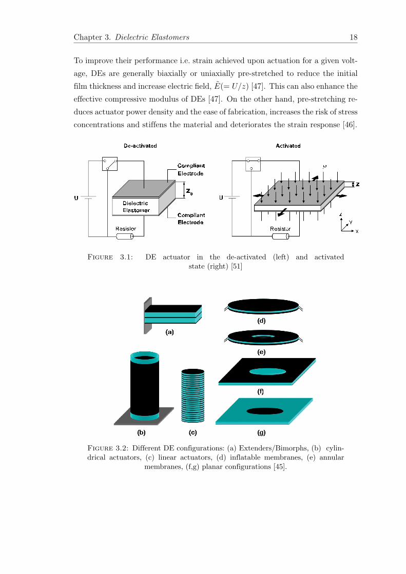
Figure 3.1 demonstrates the actuation principle of a DE.
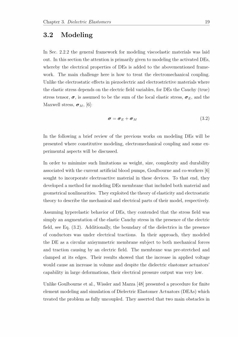
Based on their required application, DEs come into variety of shapes [45] such
as: inflated membrane (circular) configuration, cylindrical configuration, annular
configuration, and planar configuration. Figure 3.2 illustrates these configurations [45].
1They are called compliant since they allow the dielectric to deform without affecting itsmechanical performance [49].
Chapter 3. Dielectric Elastomers 18
To improve their performance i.e. strain achieved upon actuation for a given volt-
age, DEs are generally biaxially or uniaxially pre-stretched to reduce the initial
film thickness and increase electric field, E(= U/z) [47]. This can also enhance the
effective compressive modulus of DEs [47]. On the other hand, pre-stretching re-
duces actuator power density and the ease of fabrication, increases the risk of stress
concentrations and stiffens the material and deteriorates the strain response [46].
Figure 3.1: DE actuator in the de-activated (left) and activatedstate (right) [51]
Figure 3.2: Different DE configurations: (a) Extenders/Bimorphs, (b) cylin-drical actuators, (c) linear actuators, (d) inflatable membranes, (e) annular
membranes, (f,g) planar configurations [45].
Chapter 3. Dielectric Elastomers 19
3.2 Modeling
In Sec. 2.2.2 the general framework for modeling viscoelastic materials was laid
out. In this section the attention is primarily given to modeling the activated DEs,
whereby the electrical properties of DEs is added to the abovementioned frame-
work. The main challenge here is how to treat the electromechanical coupling.
Unlike the electrostatic effects in piezoelectric and electrostrictive materials where
the elastic stress depends on the electric field variables, for DEs the Cauchy (true)
stress tensor, σ, is assumed to be the sum of the local elastic stress, σE, and the
Maxwell stress, σM , [6]:
σ = σE + σM (3.2)
In the following a brief review of the previous works on modeling DEs will be
presented where constitutive modeling, electromechanical coupling and some ex-
perimental aspects will be discussed.
In order to minimize such limitations as weight, size, complexity and durability
associated with the current artificial blood pumps, Goulbourne and co-workers [6]
sought to incorporate electroactive material in these devices. To that end, they
developed a method for modeling DEs membrane that included both material and
geometrical nonlinearities. They exploited the theory of elasticity and electrostatic
theory to describe the mechanical and electrical parts of their model, respectively.
Assuming hyperelastic behavior of DEs, they contended that the stress field was
simply an augmentation of the elastic Cauchy stress in the presence of the electric
field, see Eq. (3.2). Additionally, the boundary of the dielectrics in the presence
of conductors was under electrical tractions. In their approach, they modeled
the DE as a circular axisymmetric membrane subject to both mechanical forces
and traction causing by an electric field. The membrane was pre-stretched and
clamped at its edges. Their results showed that the increase in applied voltage
would cause an increase in volume and despite the dielectric elastomer actuators’
capability in large deformations, their electrical pressure output was very low.
Unlike Goulbourne et al., Wissler and Mazza [48] presented a procedure for finite
element modeling and simulation of Dielectric Elastomer Actuators (DEAs) which
treated the problem as fully uncoupled. They asserted that two main obstacles in
Chapter 3. Dielectric Elastomers 20
Finite Element (FE) modeling and simulation of electroactive polymers presented
themselves as the actuation modeling and the proper definition of the constitutive
equation. Although the presence of electrical field would lead to electromechanical
coupling, their approach was to solve the problem as fully uncoupled, simplifying
it to a pure mechanical problem.
Using acrylic elastomer VHB 4910 (3M) as the base material for dielectric elas-
tomer, their research work was a combination of experiments and finite element
modeling of a biaxially pre-strained actuator. They first performed series of ex-
periments such as relaxation test, tensile test and circular strain test, the result
of which were later employed to validate the numerical calculations. In their work
large strain response was modeled using strain energy potential of Yeoh [52] and
the so-called Prony series to describe the time dependence of the mechanical re-
sponse. The outcome of their work demonstrated a good agreement between FE
calculation and experiment and highlighted the importance of multi-axial testing
in determining the proper constitutive models for DEs. Finally, Wissler and Mazza
pointed out that main drawback of their proposed procedure was the treatment of
the problem as an uncoupled problem where the voltage was incorporated as the
output of the calculation.
In the meantime, Kofod and Sommer-Larsen [4], reviewed the present situation
in the theory of DEAs aiming at providing an insight into the actuation models
and electromechanical coupling background. They proposed non-linear high-strain
model requiring only elastic stresses and Maxwell stresses and wrapped up their
review with some comments on the improvement of DEs.
Choi et al. [53] proposed a new biomimetic DEAs design called ANTLA (AN-
Tagonistically driven Linear Actuator) with such applications as earthworms or
maworms when used as a microrobot. Using these actuators they were seeking to
achieve four typical states of human muscles; namely, forward, backward, highly
compliant and highly stiff. Satisfying major features of a muscle-like actuator
i.e. bidirectional actuation and compliance controllability, their proposed design
was composed of a prestretched elastomer film foiled on the frame, which was
engaged with uniform pretension along the direction of actuation. Modeling both
statically and dynamically, Choi and co-workers applied their design to a proto-
type aiming at verifying the effectiveness of the modeling techniques as well as
the control method. They finally argued that by changing some parameters, their
presented idea could result in a paradigm of design in robotics.
Chapter 3. Dielectric Elastomers 21
Motivated by the increasing interest in using the electromechanical devices based
on polymer coated with compliant electrodes, Begley et al. [54] investigated, both
theoretically and experimentally, the coupling electrical input and out-of-plane
behavior of silicon-based multilayered DEAs in 2005. Their work was aimed at
providing (1) “experimental validation of constitutive theories for cracked lami-
nates”, (2) “experimental validation of closed form membrane load-deflection so-
lutions that involved strain”, and (3) “the complete mechanics framework needed
to extract toughness values for nanoscale films from membrane stretching experi-
ments”. Using the Begley-Mackin membrane deflection model [55] to extract both
the effective modulus of the cracked multilayer, and electrically induced strain,
they asserted that their proposed models were capable of predicting the coupled
electromechanical response of previously described DEAs. They, also, indicated
that electrode cracking should be promoted since it decreases the effective modulus
of multilayer and improved charge distribution due to smaller crack openings.
Carpi and De Rossi [56], however, presented findings of their research activities in
developing soft actuators made of silicon-based DEs with the potential applications
as artificial muscles. In this regard, they introduced three applications; namely,
eyeballs of an android robotic face, an anthropomorphic skeleton of upper limb, as
well as a new robotic endoscope and investigated the actuation principle of these
devices. They argued that despite such excellent features as sizable active strains
and/or stresses in response to an electrical stimulus, low specific gravity, high grade
of processability, down-scalability, and low costs, DEs required high driving electric
fields (order of 10 - 100 V/µm) which prevented them from utilization in any
intrabody applications. This problem could, however, be rectified by development
of new improved materials and configurations which required lower driving voltage.
Seeking to establish a basis for the design of DEAs, Koo et al. [44] suggested
an actuator controlled by an antagonistic drive mechanism, and examined the
pre-strain effect on the actuation mechanism. Adopting Mooney-Rivlin theory
describing the constitutive relation, they carried out the numerical analysis and
verified their proposed design through an experiment.
Meanwhile, Mockensturm and Goulbourne [57] examined the dynamic behavior
of one of the simplest possible DEs configurations i.e. an axisymmetric spherical
inflated membrane subject to an electric field. Using the Mooney material model,
the result of their work showed that the actuation of DEAs should be feasible
with electric fields well below the breakdown field of the dielectric. Maintaining
Chapter 3. Dielectric Elastomers 22
the mechanical pressure constant during rapid inflation, they argued that despite
the limited usefulness of such actuators due to their characteristics, they were
still a good substitute to be exploited as an auxiliary device in the cardiovascular
system.
In 2007, Patrick et al. [51] conducted a research aimed at examining the perfor-
mance of planar DEAs under certain boundary conditions for quasi-static acti-
vation cycles. They modeled hyperelastic DEs using a three-dimensional coupled
spring system which was equivalent to the constitutive model developed by Ogden.
As for the electromechanical coupling applicable to their proposed DEAs, Patrick
and co-workers introduced the equivalent electrode pressure in the thickness di-
rection which covered two electromechanical effects; namely, (1) squeeze of the
film by the electrodes due to the attraction of opposing charges in the thickness
direction and (2) planar expansion of the film as a result of the repelling forces
between equal charges on two electrodes. They further asserted that for DE two
kinds of activation existed: activation with constant charge2 and activation with
constant voltage3; while the former led to only one equilibrium state, the latter
predicted two equilibrium (stable and unstable) states. Introducing the critical
voltage, they also suggested an electromechanical collapse should the voltage ex-
ceeded the critical value. And they finally concluded that the pre-stretching of
DEs would lead to improved performance at lower initial activation field.
In the meantime, Plante and Dubowsky [58] highlighted the results of their study
on the performance of DEAs in practical applications and proposed a design
space considering pull-in failure, dielectric strength failure, viscoelasticity and cur-
rent leakage as four major governing mechanisms. They developed an analytical
model based on hyperelastic and Bergstrom-Boyce viscoelastic material models
and verified the performance of DEAs over a range of actuation velocities. Dis-
cussing the possible applications of their design in robotics and mechantronics,
Plante and Dubowsky compared such actuators with their electromagnetic coun-
terparts.
Wissler and Mazza [1], however, investigated the electromechanical coupling in
DEs both analytically and numerically in 2007. They conducted series of experi-
ments on such actuators with different dielectric constants and prestretch ratio in
order to validate their theoretical approach. The results of their work indicated a
2In this case the source is disconnected from the actuator after its initial electrical charging[51].3In this case the source remains connected to the actuator during its active deformation [51].
Chapter 3. Dielectric Elastomers 23
consistency between the analytical and numerical assumptions and succeeded to
verify the suggested equation of Pelrine [59] through theory and experiment.
Seeking to comprehend the major performance mechanisms of DEAs made of VHB
4905/4910 from 3M, Plante and Dubowsky [60] carried out an experimental in-
vestigation to portray the actuator performance in terms of force, power, current
consumption, work output, and efficiency. They modeled the viscoelastic behav-
ior of DEAs using a Mooney-Rivlin model in conjunction with Bergstrom-Boyce
model. The result of their study revealed that viscoelasticity and current leakage
were the restricting parameters for designing a DEA.
Motivated by the limited experimental efforts on the dynamic response analysis
of DEAs, Fox and Goulbourne [49] conducted series of experiments in 2008. They
performed their experiment on inflating planar DEs clamped-edge circular mem-
branes. Owing to this fact, they centered their attention to enlarge these areas and
experimentally quantify the large deformation dynamic behavior of DEAs mem-
brane. To that end they prepared test specimen of their work by prestretching the
commercially available VHB 4905 DE and fixing it in the test chamber as well as
applying carbon grease as the compliant electrode on either sides of the membrane.
Fox and Goulbourne later applied sinusoidal voltage (time-varying voltage) signals
to a DEA and then varied harmonically the volume inside the test chamber using
a piston pump (time-varying pressure loads). Using these experiments, one could
achieve a pumping action by cycling the inflation and deflation of the membrane
through constantly applying and removing the electric field. The results of their
study indicated that the dynamic behavior of DEAs was the direct consequence of
the classical dynamic response of membranes with all the attributes e.g. damping
coefficients and mode-shapes. For DEAs all parts of the system, however, did not
pass through the equilibrium simultaneously.
Fox and Goulbourne [61] highlighted the outcomes of a comprehensive experimen-
tal investigation intended to illustrate the dynamic deformation response of DE
membranes. These membranes were fixed at their outer edge and subjected to a
dynamic electric field and such variable systems parameters as chamber volume,
initial flat state, and voltage offset. The numerical procedure of their work was
based on the elastic membrane theory of Green and Adkins [62] and the electro-
static Maxwell stress effect. The numerical procedure was further calibrated with
experimental data from inflation quasi-static tests of the DE membranes. It was
evident from their work that electrical excitation of resonance phenomena could be
Chapter 3. Dielectric Elastomers 24
utilized in actuation applications, and the electric field could be used to transform
a smooth monolithic structure into specific symmetry surface patterns which had
a major advantage for adaptive structures. In addition they pointed out that the
chamber volume was an important system parameter in dynamic DEs actuation.
More recently and motivated by the lack of published models for cone DEAs,
Wang et al. [50] published a paper describing the finite element simulation, the
manufacturing and the analysis of the working principle of such actuators. They
applied Yeoh hyperelastic model for the finite element simulation used to predict
the movement of the actuator. They, finally, pointed out that high active voltage
was a major barrier in development of DEAs with real life applications.
3.3 Experiments
This section intends to provide a short overview of experiments with DEs. These
experiments are aimed at providing electromechanical behavior of these materi-
als [45]. In general experimental works with DEs fall into these two categories [45]:
(1) quasi-static experiments and (2) dynamics experiments.
Quasi-static experiments consist of uniaxial compression tests, tensile tests,
and biaxially pre-strained circular actuator experiments [48, 63]. The first two tests
are served to provide such material parameters as compressive moduli and tensile
moduli, while the biaxial pre-strained test are usually performed after the first
two tests is used to mimic the electrical actuation conditions between compliant
electrodes [63].
Dynamic experiments, on the other hand, are exploited to study the dynamic
response of DEs. They comprise of dynamic mechanical loading experiments and
dynamic electrical loading experiments. While the former is carried out using a dy-
namic pressure input, the latter measures the dynamic electrical loading response
due to a dynamic voltage input [45]. For an extensive coverage of the experimental
procedures and set-up associated with DEs the interested readers are referred to
Ref. [45]
Chapter 3. Dielectric Elastomers 25
3.4 Applications
To wrap up this chapter some major applications of DEs as appeared in [64] are
presented. One can find DEs’ presence in such application areas as (1) biomedicine
with haptic and micro-scale applications, (2) robotics with biorobotic applications
and (3) industry with commercial applications.
Examples of biomedical applications include orthotics and prosthetics, force feed-
back devices, microactuators, micro-optics, and a new Braille displaye system
design [64]. Biommimetic robots, micro-annelid-like robot actuated by artificial
muscles, binary actuators, robotic arm, on the other hand, can be mentioned as
some of the applications of DEs in Robotics. And finally loudspeakers are a good
example of DEs commercial application.
Chapter 4
Modeling of Dielectric Elastomers
4.1 Introduction to Nonlinear Analysis
In the following a rather brief introduction to nonlinear analysis will be presented.
The facts and theories throughout this chapter are adopted from Ref. [65–70].
Most problems in solid mechanics are nonlinear in nature. Linear assumptions
would only result in approximate solutions which, often, do not represent the
actual behavior of the system. In order to study the nonlinear behavior of the
mechanical systems it is necessary to first classify different sources of nonlinearities.
In this regard geometrical nonlinearities, material nonlinearities and nonlinear
boundary conditions comprise the sources of nonlinearities.
Geometrical nonlinearities are accounted for in situations where a solid reaches a
state for which undeformed and deformed shapes are substantially different [65].
Typical examples of geometrical nonlinearities are structural instability analyses,
forming processes, crash and impact problems.
Material nonlinearities, however, stem themselves from the nonlinear stress-strain
behavior in the constitutive model of the material [66]. Relevant nonlinear material
models include nonlinear (hyper-) elasticity, plasticity, viscoelasticity, creep and
damage.
Nonlinear boundary conditions, on the other hand, are the result of large deforma-
tion [66]. Examples of such nonlinearities are pressure loadings that remain normal
to the deformed body and also the case where the deformed boundary interacts
26
Chapter 4. Modeling of Dielectric Elastomers 27
with another body, i.e. contact problems [65]. In the current work, however, the
first two forms of nonlinearities i.e. geometrical and material nonlinearities are of
primary concerns.
In the context of the finite element method, the governing equations describing
such nonlinear behaviors are generally expressed in a weak integral form using for
example the principle of virtual work. Manipulating these integral equations yield
a finite set of nonlinear algebraic equations which are usually solved utilizing the
Newton-Raphson iterative schemes [66].
In the next sections, some pertinent aspects of nonlinear continuum mechanics
will be reviewed followed by the formulation of the constitutive equations and
finite element implementation of the presented constitutive model for dielectric
elastomers.
4.2 Nonlinear Continuum Mechanics
4.2.1 Continuum Body
A continuum body is a macroscopic system given by infinite number of particles
defining for instance a solid, a liquid, a gas or an intermediate state. It is assumed
that there is no discontinuity between the particles and the mathematical func-
tions describing the motion and properties of the continuum body are continuous
functions.
The concept of configuration is the necessary tool to derive further equations de-
scribing kinematics and motion of a continuum body. At each instance of time t, a
continuum body occupies a different region in space referring here to as Ωt which by
reference to a suitable set of coordinate system is said to specify the configuration
of the continuum body at that instance of time. The configuration Ω0 at t = 0
is commonly referred to as reference or material configuration, while any other
configuration at time t > 0 is called current, spatial or deformed configuration.
Current and reference configurations can be converted to each other through the
so-called the motion mapping and the inverse motion mapping. Denoting X as
the position vector of a particle P in reference configuration and x as the position
Chapter 4. Modeling of Dielectric Elastomers 28
vector of a particle P in current configuration, the motion mapping is defined as:
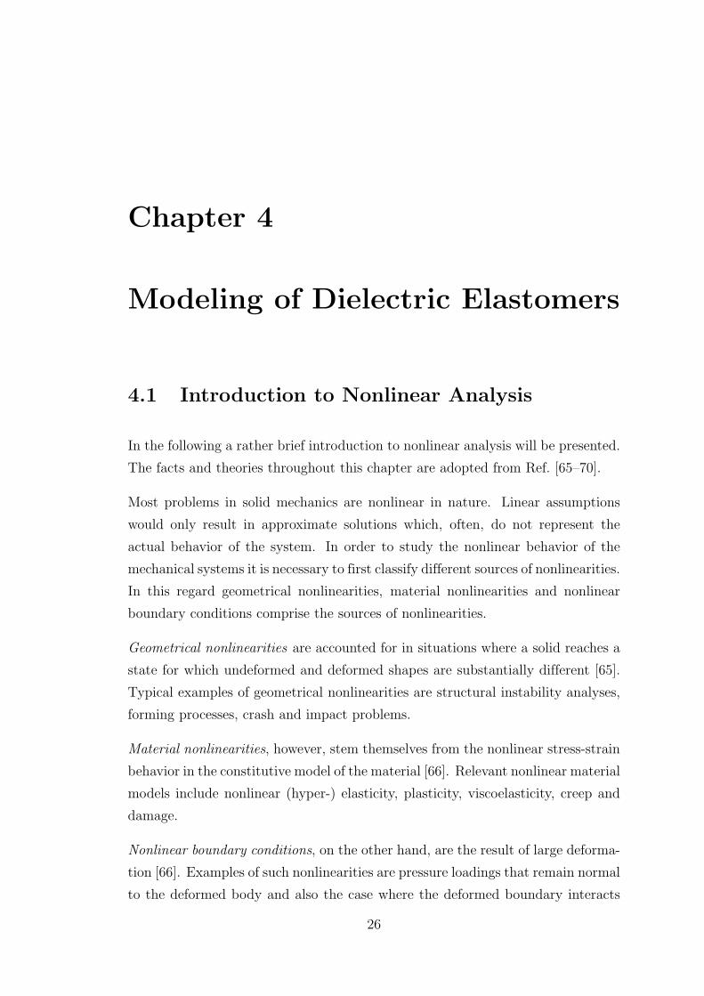
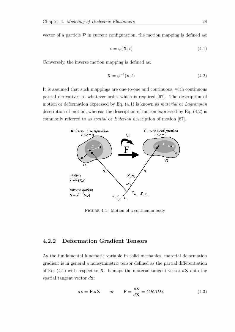
x = ϕ(X, t) (4.1)
Conversely, the inverse motion mapping is defined as:
X = ϕ−1(x, t) (4.2)
It is assumed that such mappings are one-to-one and continuous, with continuous
partial derivatives to whatever order which is required [67]. The description of
motion or deformation expressed by Eq. (4.1) is known as material or Lagrangian
description of motion, whereas the description of motion expressed by Eq. (4.2) is
commonly referred to as spatial or Eulerian description of motion [67].
Figure 4.1: Motion of a continuum body
4.2.2 Deformation Gradient Tensors
As the fundamental kinematic variable in solid mechanics, material deformation
gradient is in general a nonsymmetric tensor defined as the partial differentiation
of Eq. (4.1) with respect to X. It maps the material tangent vector dX onto the
spatial tangent vector dx:
dx = F.dX or F =dx
dX= GRADx (4.3)
Chapter 4. Modeling of Dielectric Elastomers 29
The inverse deformation gradient, on the other hand, is defined as the partial
differentiation of Eq. (4.2) with respect to x. It maps the spatial tangent vector
dx onto the material tangent vector dX:
dX = F−1.dx or F−1 =dX
dx= gradX (4.4)
4.2.3 Strain Tensors
In nonlinear continuum mechanics such strain tensors as Green-Lagrange and
Euler-Almansi strain tensors are introduced in order to establish a relation be-
tween the undeformed (reference) and deformed (current) configurations.
Green-Lagrange strain tensor, E, is a material symmetric second order tensor
which is deduced when the deformation is measured as the difference between
the square of the spatial length, dl, and the material length, dL. Expressing the
square of the spatial length as dl2 = dx.dx and the square of the material length
as dL2 = dX.dX, one has:
dl2 − dL2 = dx.dx − dX.dX
= FdX.FdX − dX.dX
= dXFTFdX − dX.dX
= dX.(FTF − I)dX
= 2dX.E.dX
Green-Lagrange strain tensor, E, is then defined as:
E :=1
2(FTF − I) (4.5)
where, I is the second-order identity tensor:
I =
1 0 0
0 1 0
0 0 1
(4.6)
Euler-Almansi strain tensor, e, on the other hand, is a spatial symmetric sec-
ond order tensor which is also derived when the deformation is measured as the
difference between the square of the spatial length, dl, and the material length,
Chapter 4. Modeling of Dielectric Elastomers 30
dL. Expressing the square of the spatial length as dl2 = dx.dx and the square of
the material length as dL2 = dX.dX, one has:
dl2 − dL2 = dx.dx − dX.dX
= dx.dx − F−1dxF−1dx
= dx.dx − dxF−TF−1dx
= dx.(I − F−TF−1)dx
= 2dx.e.dx
Euler-Almansi strain tensor, e, is then defined as:
e :=1
2(I − F−TF−1) (4.7)
4.2.4 The Concept of Stress
Prior to the introduction of the concept of stress in continuum mechanics it is nec-
essary to have a basic understanding of some other preliminary concepts. First,
forces acting on a continuum body are discussed. In the context of nonlinear con-
tinuum mechanics, two types of forces; namely, body forces and surface forces, are
usually considered. Body forces also known as internal forces act within a contin-
uum body. Typical examples of such forces are the gravity forces, electromagnetic
forces, etc. On the contrary, surface forces act on outer boundary of a continuum
body. Contact forces between bodies or applied forces on the surface of a body
are some examples of surface forces.
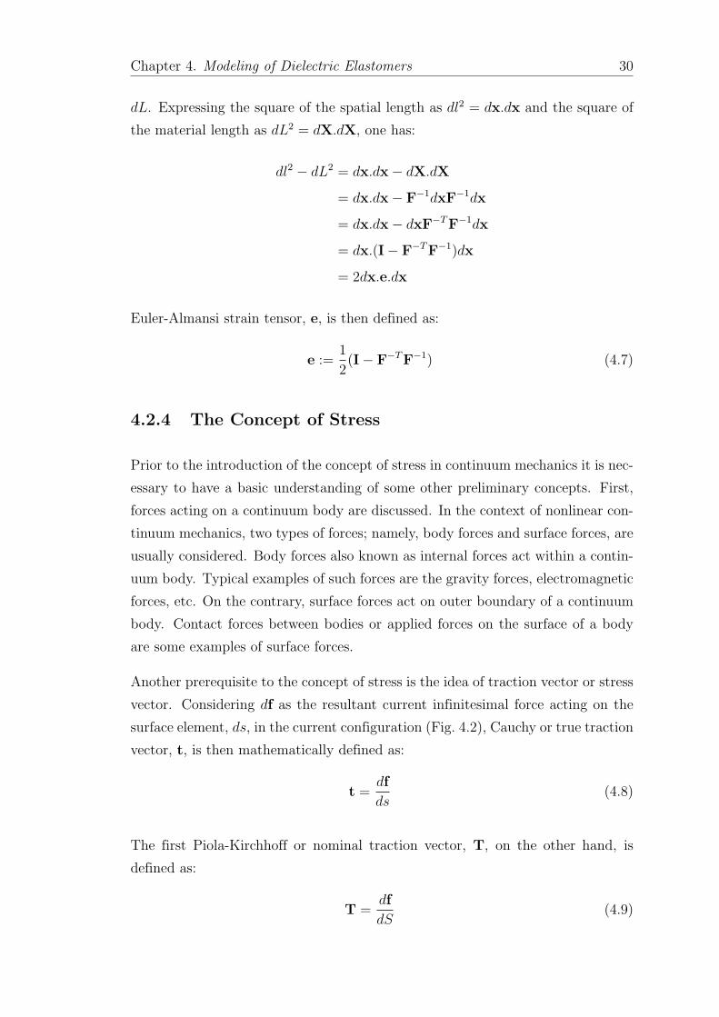
Another prerequisite to the concept of stress is the idea of traction vector or stress
vector. Considering df as the resultant current infinitesimal force acting on the
surface element, ds, in the current configuration (Fig. 4.2), Cauchy or true traction
vector, t, is then mathematically defined as:
t =df
ds(4.8)
The first Piola-Kirchhoff or nominal traction vector, T, on the other hand, is
defined as:
T =df
dS(4.9)
Chapter 4. Modeling of Dielectric Elastomers 31
Where, dS is the surface element in the reference configuration.
Figure 4.2: Traction vector
By the introduction of the abovementioned preliminaries, it is now possible to
present the definition of the stress tensors in a continuum body. By virtue of
the Cauchy’s stress principle, one can associate the true traction vector, t, at an
arbitrary point inside the continuum body to the unit normal vector, n, in the
current configuration as illustrated in Fig. 4.2. This leads to the definition of the
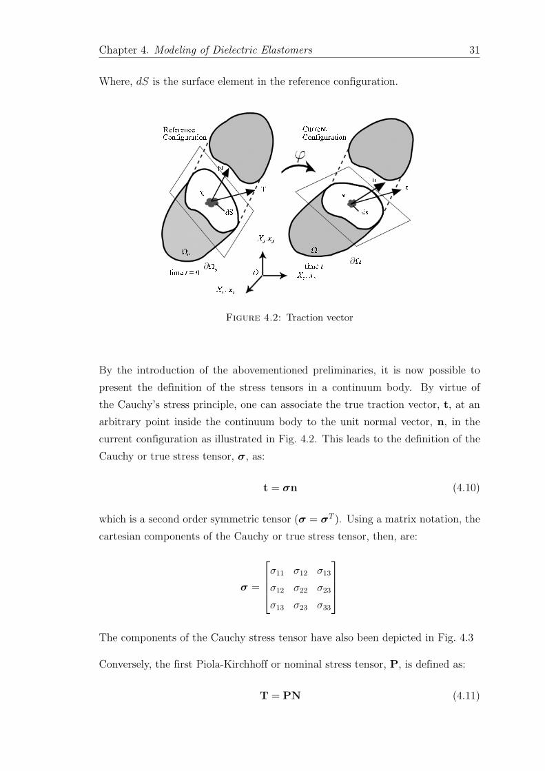
Cauchy or true stress tensor, σ, as:
t = σn (4.10)
which is a second order symmetric tensor (σ = σT ). Using a matrix notation, the
cartesian components of the Cauchy or true stress tensor, then, are:
σ =
σ11 σ12 σ13
σ12 σ22 σ23
σ13 σ23 σ33
The components of the Cauchy stress tensor have also been depicted in Fig. 4.3
Conversely, the first Piola-Kirchhoff or nominal stress tensor, P, is defined as:
T = PN (4.11)
Chapter 4. Modeling of Dielectric Elastomers 32
Figure 4.3: Cauchy’s stress tensor components
Where N is the unit normal vector in the reference configuration. These two stress
tensors are related to each other through the following expression:
σ =1
detFPFT (4.12)
Other stress tensors which are worth mentioning here are the second Piola-Kirchhoff
and Kirchhoff stress tensors. The second Piola-Kirchhoff stress tensor, S, is related
to the Cauchy stress tensor as:
S = detF F−1σ F−T (4.13)
While, Kirchhoff stress tensor, τ , is related to Cauchy stress tensor such that:
τ = detF σ (4.14)
It is also worth mentioning that for each one of the abovementioned stress ten-
sors there is an energetically conjugate strain tensor provided that the (virtual)
energy is not affected by the choice of a certain pair of stresses and strains. In
this regard, second Piola-Kirchhoff stresses and Green-Lagrange strains are ener-
getically conjugate. Other energetically conjugate pairs of stresses and strains are:
deformation gradient and first Piola-Kirchhoff stresses, Euler-Almansi strains and
Cauchy stresses.
Chapter 4. Modeling of Dielectric Elastomers 33
4.3 Infinitesimal Strain Theory
4.3.1 General Overview
Since the analyses associated with the current study are mostly based on the
infinitesimal (small) strain theory, it is essential to introduce the basic assumptions
used therein. These include:
1. No distinction between current (deformed) configuration and reference configuration
is considered:
Ω0∼= Ω (4.15)
2. No distinction between material coordinates (at the reference configuration)
and spatial coordinates (at the current deformed configuration) is considered:
x = X (4.16)
3. No distinction between material and spatial descriptions is considered.
4. No difference between material and spatial differential operators (e.g. gra-
dient and divergence) is considered.
One of the direct consequences of the infinitesimal strain theory is that all the
strain tensors are considered the same, given by:
ε := sym[∇u] =1
2[∇u + ∇uT ] (4.17)
where u is the displacement tensor.
4.3.2 Voigt-Notation
Taking advantage of the symmetric properties of the stress and strain tensors1,
it is always more practical to exploit the so-called Voigt-Notation instead of the
1The symmetric properties of stresses come from the balance of angular momentum while thesymmetric properties of strains is the consequence of infinitesimal strain assumption.
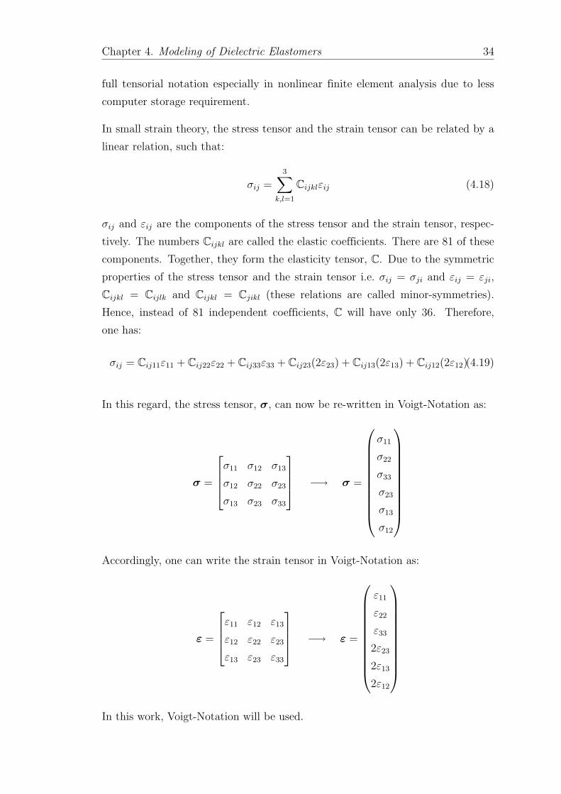
Chapter 4. Modeling of Dielectric Elastomers 34
full tensorial notation especially in nonlinear finite element analysis due to less
computer storage requirement.
In small strain theory, the stress tensor and the strain tensor can be related by a
linear relation, such that:
σij =3∑
k,l=1
Cijklεij (4.18)
σij and εij are the components of the stress tensor and the strain tensor, respec-
tively. The numbers Cijkl are called the elastic coefficients. There are 81 of these
components. Together, they form the elasticity tensor, C. Due to the symmetric
properties of the stress tensor and the strain tensor i.e. σij = σji and εij = εji,
Cijkl = Cijlk and Cijkl = Cjikl (these relations are called minor-symmetries).
Hence, instead of 81 independent coefficients, C will have only 36. Therefore,
one has:
σij = Cij11ε11 + Cij22ε22 + Cij33ε33 + Cij23(2ε23) + Cij13(2ε13) + Cij12(2ε12)(4.19)
In this regard, the stress tensor, σ, can now be re-written in Voigt-Notation as:
σ =
σ11 σ12 σ13
σ12 σ22 σ23
σ13 σ23 σ33
−→ σ =
σ11
σ22
σ33
σ23
σ13
σ12
Accordingly, one can write the strain tensor in Voigt-Notation as:
ε =
ε11 ε12 ε13
ε12 ε22 ε23
ε13 ε23 ε33
−→ ε =
ε11
ε22
ε33
2ε23
2ε13
2ε12
In this work, Voigt-Notation will be used.
Chapter 4. Modeling of Dielectric Elastomers 35
4.3.3 Spherical and Deviatoric Tensors
In nonlinear continuum mechanics, a strain tensor can be viewed as an additive
split of the so-called volumetric and deviatoric parts. Volumetric strain, e, also
known as spherical strain is a scalar quantity which describes the dilatation or
the relative variation of the volume in the continuum body. It is mathematically
defined as the trace of the strain tensor:
e := tr[ε] = ε11 + ε22 + ε33 (4.20)
The deviatoric part of the strain, ε′, also known as isochoric strain is the volume
preserving strain and is defined as:
ε′ = ε −1
3tr[ε]I (4.21)
where, I, is the second-order identity tensor.
Accordingly, the stress tensor can be viewed as an additive split of the spherical
part and deviatoric part such that:
σesp =1
3tr[σ]I (4.22)
is the spherical part of the stress, and
σ′ = σ −1
3tr[σ]I (4.23)
is the deviatoric part of the stress.
4.4 Balance Laws
Balance laws as well as some restriction principles, e.g. second law of thermo-
dynamics are required to derive the governing equations of a continuum body.
The resulting system of equations, however, can only be solved in conjunction
with kinematic relation, as explained in the previous sections, and constitutive
equations.
Chapter 4. Modeling of Dielectric Elastomers 36
Balance laws can mathematically be expressed in either the integral (global) form
or the strong (local) form. Each one of these representations can also be cast
either in reference (material) or current (spatial) configurations. These laws in-
clude, Conservation of Mass, Balance of Linear Momentum, Balance of Angular
Momentum, Energy Balance along with the Second Law of Thermodynamics as
the restriction.
Conservation of Mass states that during a motion there are neither mass sources
nor mass sinks and the mass, m, of a continuum body is conserved. The global
and local spatial forms of conservation of mass can, therefore, be expressed as
Eq. (4.24) and Eq. (4.25), respectively:
d
dt
∫
Ω
ρ dv = 0 (4.24)
∂ρ
∂t+ ρ(divv) = 0 (4.25)
Where, ρ is the density, v is the volume of the continuum body, Ω, and v is the
velocity.
Balance of Linear Momentum states that the time-variation of the linear
momentum of a material volume is equal to the resultant force acting on the
material volume. The global and local spatial forms of balance of linear momentum
are presented as, Eq. (4.26) and Eq. (4.27), respectively.
d
dt(ML) = F (4.26)
ρ∂v
∂t= div[σ] + ρb (4.27)
where F =∫
Ωρb dΩ+
∫
∂Ωt d∂Ω. Here b represents the body forces, t is the traction
vector, and ∂Ω is the surface area of the continuum body.
Balance of Angular Momentum, on the other hand, states that the time-
variation of the angular momentum of a material volume with respect to a fixed
point, MO, is equal to the resultant moment with respect to this fixed point, M.
The global and local spatial forms of balance of angular momentum are presented
Chapter 4. Modeling of Dielectric Elastomers 37
as, Eq. (4.28) and Eq. (4.29), respectively.
d
dt(MO) = M or
d
dt
∫
Ω
r × ρv dΩ =
∫
Ω
r × ρb dΩ +
∫
∂Ω
r × t d∂Ω (4.28)
σ = σT (4.29)
where, r = x−x0, is the distance from point O. The Equation (4.29) is interpreted
as the symmetry of the Cauchy stress tensor.
Balance of Energy states that the material time derivative of the total energy
of the system is equal to the External Mechanical Power and External Thermal
Power. Defining external mechanical power as:
Pext :=
∫
Ω
ρb · v dΩ +
∫
∂Ω
t · v d∂Ω (4.30)
and external thermal power as:
Qext :=
∫
Ω
ρr dΩ −
∫
∂Ω
q · n d∂Ω (4.31)
Balance of energy is mathematically expressed as:
d
dt(E + K) = Pext + Qext (4.32)
where E is the internal energy, K is the kinetic energy, and q is the spatial heat
flux per unit of spatial surface area, ∂Ω, in the current configuration.
The First Law of Thermodynamics states that the material time derivative
of the total energy is equal to the material time derivatives of the kinetic and
internal energy. This can be mathematically presented as:
ρe = σ : ε + ρr − divq (4.33)
where e is the internal energy per unit mass and r is the internal heat source rate
per unit of mass.
The Second Law of Thermodynamics states that the material time derivative
of the entropy, H, must always be greater or equal to the rate of the entropy input
into the system. The rate of the entropy , η, is defined as the rate of the total
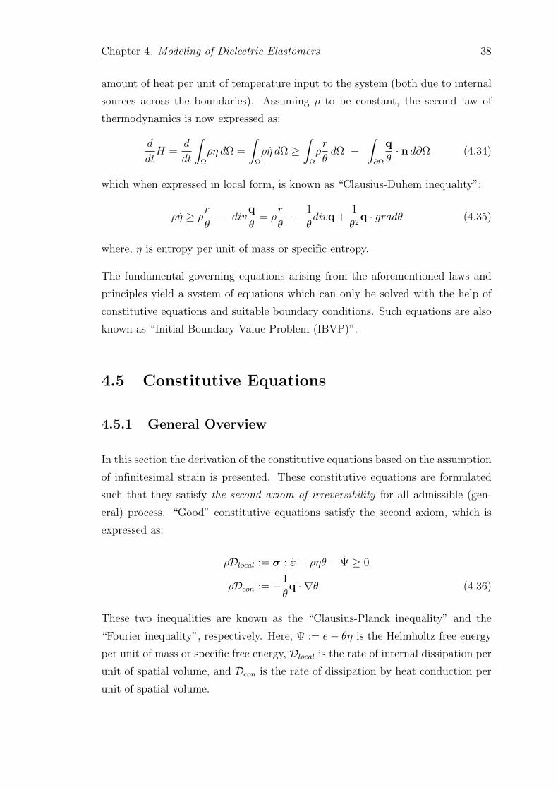
Chapter 4. Modeling of Dielectric Elastomers 38
amount of heat per unit of temperature input to the system (both due to internal
sources across the boundaries). Assuming ρ to be constant, the second law of
thermodynamics is now expressed as:
d
dtH =
d
dt
∫
Ω
ρη dΩ =
∫
Ω
ρη dΩ ≥
∫
Ω
ρr
θdΩ −
∫
∂Ω
q
θ· n d∂Ω (4.34)
which when expressed in local form, is known as “Clausius-Duhem inequality”:
ρη ≥ ρr
θ− div
q
θ= ρ
r
θ−
1
θdivq +
1
θ2q · gradθ (4.35)
where, η is entropy per unit of mass or specific entropy.
The fundamental governing equations arising from the aforementioned laws and
principles yield a system of equations which can only be solved with the help of
constitutive equations and suitable boundary conditions. Such equations are also
known as “Initial Boundary Value Problem (IBVP)”.
4.5 Constitutive Equations
4.5.1 General Overview
In this section the derivation of the constitutive equations based on the assumption
of infinitesimal strain is presented. These constitutive equations are formulated
such that they satisfy the second axiom of irreversibility for all admissible (gen-
eral) process. “Good” constitutive equations satisfy the second axiom, which is
expressed as:
ρDlocal := σ : ε − ρηθ − Ψ ≥ 0
ρDcon := −1
θq · ∇θ (4.36)
These two inequalities are known as the “Clausius-Planck inequality” and the
“Fourier inequality”, respectively. Here, Ψ := e − θη is the Helmholtz free energy
per unit of mass or specific free energy, Dlocal is the rate of internal dissipation per
unit of spatial volume, and Dcon is the rate of dissipation by heat conduction per
unit of spatial volume.

Chapter 4. Modeling of Dielectric Elastomers 39
The formulation of the constitutive equations, here, follows the general internal
variable formulation, where a generalized vector I ∈ Rn of internal variable is,
first, introduced (e.g. viscous strain, εs, plastic strain, εp, · · · ). Two funda-
mental constitutive functions are, further, exploited, i.e. Energy Storage func-
tion, Ψ, and Dissipation function, Φ. The former governs the storage mechanics
(“spring”) whereas the latter governs the dissipative mechanism. This is illustrated
in Fig. 4.4.
Figure 4.4: Material box
These two functions govern a broad class of inelastic material models and using
the so-called “Coleman’s Exploitation Method”, one can derive the constitutive
equations. This is demonstrated as follows:
assuming,
Ψ = Ψ(ε, θ, I) (4.37)
and
Φ = Φ(F) (4.38)
the Clausius–Planck ineqaulity can be re-written as:
ρDlocal = [σ − ρ∂εΨ] : ε − ρ[η + ∂σΨ] · θ − ρ∂IΨ · I ≥ 0 (4.39)
This procedure will ensure the thermodynamic consistency of the material model.
Chapter 4. Modeling of Dielectric Elastomers 40
Using the Coleman’s Exploitation Method yields the following constitutive equa-
tions for stresses, entropy and internal forces:
σ = ρ∂εΨ(ε, θ, I) (4.40)
η = −∂θΨ(ε, θ, I) (4.41)
F = ∂IΨ(ε, θ, I) (4.42)
4.5.2 3D Formulation of the Viscoelastic Constitutive Model
A three dimensional formulation of the viscoelastic constitutive model presented
here is based on the Maxwell material (Fig. 4.5) which is the most general lin-
ear viscoelastic model. Assuming a volumetric-isochoric split of strain, the two
fundamental functions for the free energy, Ψ, and dissipation functional, Φ, are
expressed as:
Ψ(ε, α1, · · · ,αn) =1
2κe2 + µ0‖ε
′‖2 +n∑
i=1
µi‖ε′ − αi‖
2 (4.43)
Φ(β1, · · · , βn) =n∑
i=1
1
2
1
ηi
‖βi‖2 (4.44)
where, αi, are the tensors of the internal variables, βi, are the tensors of the
internal forces, κ is the bulk modulus, ηi = µiτi is the viscosity of the dashpots, τi
is the relaxation time, µi is the shear modulus of the springs in the Maxwell arm,
µ0 is the ground shear modulus, e is the trace of the strain tensor, and ε′ is the
deviatoric strain.
Using the Coleman’s exploitation method, i.e. :
σ = ∂εΨ ; βi = −∂αiΨ ; αi = ∂β
iΦ (4.45)
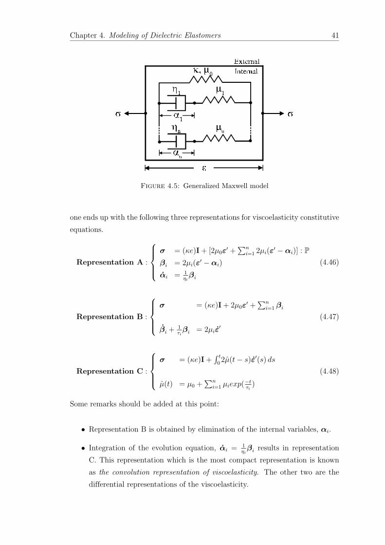
Chapter 4. Modeling of Dielectric Elastomers 41
Figure 4.5: Generalized Maxwell model
one ends up with the following three representations for viscoelasticity constitutive
equations.
Representation A :
σ = (κe)I + [2µ0ε′ +
∑n
i=12µi(ε
′ − αi)] : P
βi = 2µi(ε′ − αi)
αi = 1
ηi
βi
(4.46)
Representation B :
σ = (κe)I + 2µ0ε′ +
∑n
i=1βi
βi + 1
τi
βi = 2µiε′
(4.47)
Representation C :
σ = (κe)I +∫ t
02µ(t − s)ε′(s) ds
µ(t) = µ0 +∑n
i=1µiexp(−t
τi
)
(4.48)
Some remarks should be added at this point:
• Representation B is obtained by elimination of the internal variables, αi.
• Integration of the evolution equation, αi = 1
ηi
βi results in representation
C. This representation which is the most compact representation is known
as the convolution representation of viscoelasticity. The other two are the
differential representations of the viscoelasticity.
Chapter 4. Modeling of Dielectric Elastomers 42
• Notation ‖ε′‖2 = ε′ : ε′ is the norm of the second order deviatoric strain
tensor, ε′
• µ(t) = µ0 +∑n
i=1µiexp(−t
τi
) is the shear modulus relaxation function
• P := I− 1
3I⊗ I is the fourth order deviatoric projection tensor and is defined
as:
P =
2
3−1
3−1
30 0 0
−1
3
2
3−1
30 0 0
−1
3−1
3
2
30 0 0
0 0 0 1
20 0
0 0 0 0 1
20
0 0 0 0 0 1
2
where, I is the fourth-order identity tensor and is defined as:
I =
1 0 0 0 0 0
0 1 0 0 0 0
0 0 1 0 0 0
0 0 0 0 0 0
0 0 0 0 0 0
0 0 0 0 0 0
4.5.3 Constitutive Model for Dielectric Elastomers
As mentioned in Sec. 3.2, the main challenge in developing the constitutive equa-
tions for DEs is the treatment of the electromechanical coupling in DEs placed in
an electric field. According to Goulbourne et al. [6] the state of stress at a point
in the deformed (activated) medium is determined by (1) the local elastic state
of the medium and (2) the electrostatic effect due to the presence of an electric
field. The latter effect renders itself as the so-called “Maxwell stress”, σM , which
is defined as:
σM = ε0εrE ⊗ E − ε0εr
E2
2(4.49)
where, ε0 = 8.854 . 10−12 As
Vm
2 is the free-space permittivity, εr is the dielectric
constant of the material, E is tensor of electric field and E is the amount of electric
2Amper second per Volt meter
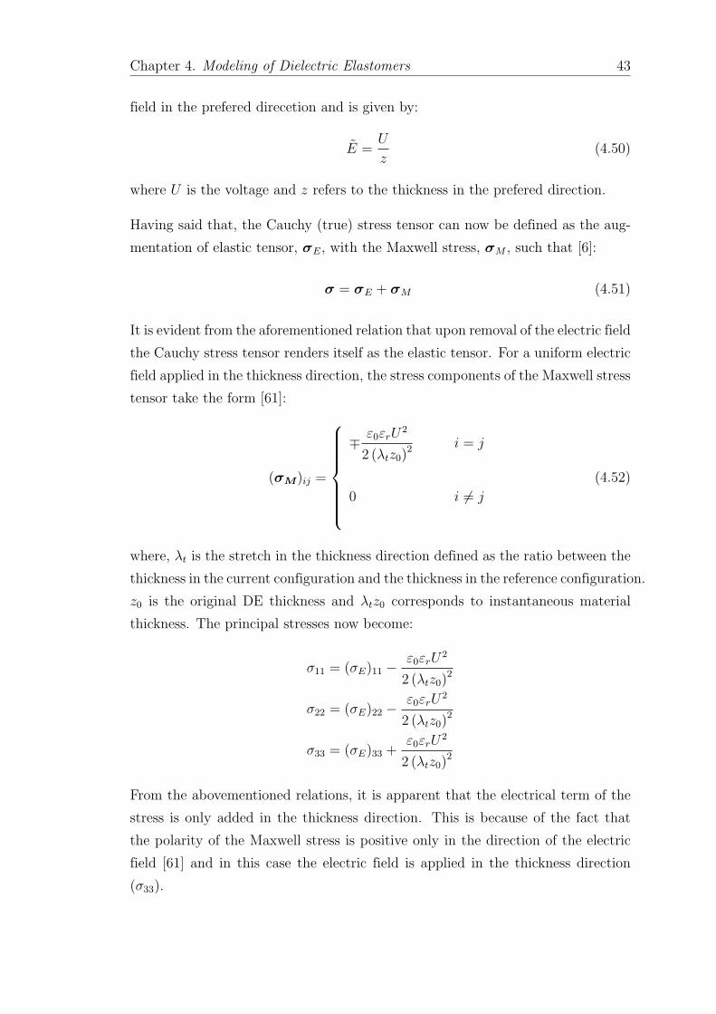
Chapter 4. Modeling of Dielectric Elastomers 43
field in the prefered direcetion and is given by:
E =U
z(4.50)
where U is the voltage and z refers to the thickness in the prefered direction.
Having said that, the Cauchy (true) stress tensor can now be defined as the aug-
mentation of elastic tensor, σE, with the Maxwell stress, σM , such that [6]:
σ = σE + σM (4.51)
It is evident from the aforementioned relation that upon removal of the electric field
the Cauchy stress tensor renders itself as the elastic tensor. For a uniform electric
field applied in the thickness direction, the stress components of the Maxwell stress
tensor take the form [61]:
(σM)ij =
∓ε0εrU
2
2 (λtz0)2
i = j
0 i 6= j
(4.52)
where, λt is the stretch in the thickness direction defined as the ratio between the
thickness in the current configuration and the thickness in the reference configuration.
z0 is the original DE thickness and λtz0 corresponds to instantaneous material
thickness. The principal stresses now become:
σ11 = (σE)11 −ε0εrU
2
2 (λtz0)2
σ22 = (σE)22 −ε0εrU
2
2 (λtz0)2
σ33 = (σE)33 +ε0εrU
2
2 (λtz0)2
From the abovementioned relations, it is apparent that the electrical term of the
stress is only added in the thickness direction. This is because of the fact that
the polarity of the Maxwell stress is positive only in the direction of the electric
field [61] and in this case the electric field is applied in the thickness direction
(σ33).
Chapter 4. Modeling of Dielectric Elastomers 44
Besides, the electrical force per unit area of the elastomer appears also as tractions
on the major surfaces [6], such that:
n · σM · n = ε0εr
E2
2(4.53)
This behavior is depicted in Fig. 4.6
Figure 4.6: Out-of-plane pressure pz and lateral stress pr acting on the dielec-tric in a circular actuator, axisymmetric view [1]
4.6 Finite Element Implementation of Linear Vis-
coelasticity
4.6.1 Finite Element Formulation of a Nonlinear Problem
The starting point for the Finite Element (FE) implementation is the principle of
“Minimum Potential Energy”. The displacement field, u is determined such that
the functional
Π(u) =
∫
Ω
Ψ(ε, θ, I) dΩ −
∫
Ω
u · ρb dΩ −
∫
∂Ω
uε d∂Ω −→ Min! (4.54)
is minimized subjected to the essential boundary conditions (i.e. u = u). In the
context of small strains, the strain tensor, ε, is defined by the following kinematic
equation:
ε := sym[∇u] =1
2[∇u + ∇uT ] (4.55)
Chapter 4. Modeling of Dielectric Elastomers 45
The variational formulation of Eq. (4.54) is obtained by the directional derivative
(first variation of Π(u)):
G(u, δu) := δΠ =d
dǫ
ǫ→0
Π(u + ǫδu) = 0
=⇒d
dǫ
ǫ→0
∫
Ω
Ψ(sym[∇(u + ǫδu)]) dΩ −
∫
Ω
(u + ǫδu) · ρb dΩ
−
∫
∂Ω
(u + ǫδu) · t d∂Ω
= 0 (4.56)
where ǫ is the eigenvalue.
Please note that sym[∇(u + ǫδu)] = ε + ǫδε. Then Eq. (4.56) can be written as:
G(u, δu) =
∫
Ω
δε : ∂εΨ(ε, θ, I) dΩ −
∫
Ω
δu · ρb dΩ −
∫
∂Ω
δu · t d∂Ω (4.57)
Equation (4.57) is the weak form of Eq. (4.54) which is called “the Principle of
Virtual Work”. Having the weak form at hand, it is now possible to continue with
the FE discretization in matrix notation. Typically in FE implementation, the
matrix notation is employed instead of the tensorial notation due to the efficient
storage and computations. The weak form is written as:
G(u, δu) =
∫
Ω
δεT · σ dΩ −
∫
Ω
δuT · ρb dΩ −
∫
∂Ω
δuT · t d∂Ω = 0 (4.58)
where the Voigt-Notation as introduced in the previous sections is applied. Here
no specification with respect to the type of element will be done. The following
approximation of the displacement field in terms of the shape function N(u) and
discrete nodal value, d is considered:
u(x) = N(x) · d ; δu(x) = N(x) · δd (4.59)
from Eq. (4.59) the strain field is computed as:
ε(x) = B(x) · d ; δε(x) = B(x) · δd (4.60)
for a 2D problem, the B-matrix has the following form:
B =
N1,x 0 N2,x 0 N3,x 0 N4,x 0
0 N1,y 0 N2,y 0 N3,y 0 N4,y
N1,y N1,x N2,y N2,x N3,y N3,x N4,y N4,x
(4.61)
Chapter 4. Modeling of Dielectric Elastomers 46
and the vector of nodal displacements looks like this:
dT =[
u1 v1 u2 v2 · · ·]
(4.62)
inserting Eq. (4.59) and (4.60) into Eq. (4.58) yields:
G(u, δu) = δdT ∫
Ω
BT · σ dΩ
︸ ︷︷ ︸
fint
−
∫
Ω
NT · ρb dΩ −
∫
∂Ω
NT · t d∂Ω
︸ ︷︷ ︸
fext
= 0 (4.63)
for arbitrary virtual displacements dT one has:
fint = fext (4.64)
where,
fint =
∫
Ω
BT · σ dΩ =n.Ele∏
e=1
∫
Ωe
BTe · σ dΩe (4.65)
fext =
∫
Ω
NT · ρb dΩ +
∫
∂Ω
NT · t d∂Ω =
n.Ele∏
e=1
∫
Ωe
NTe · ρb dΩe +
∫
∂Ωe
NTe · t d∂Ωe
(4.66)
for a general nonlinear problem, however, a residuum vector is defined as follows:
r(d) := fint − fext = 0 (4.67)
which is a set of nonlinear equations. We solve Eq. (4.67) using a typical Newton-
Raphson scheme which requires the linearization of the residuum :
Lin r(d)∣∣∣di
= r(di) +∂r
∂d
∣∣∣di
(di+1 − di)!= 0 (4.68)
the solution of Eq. (4.68) gives the update for the nodal displacement d.
d = d − (Ki)−1ri (4.69)
with
ri = fint(di) − fext (4.70)
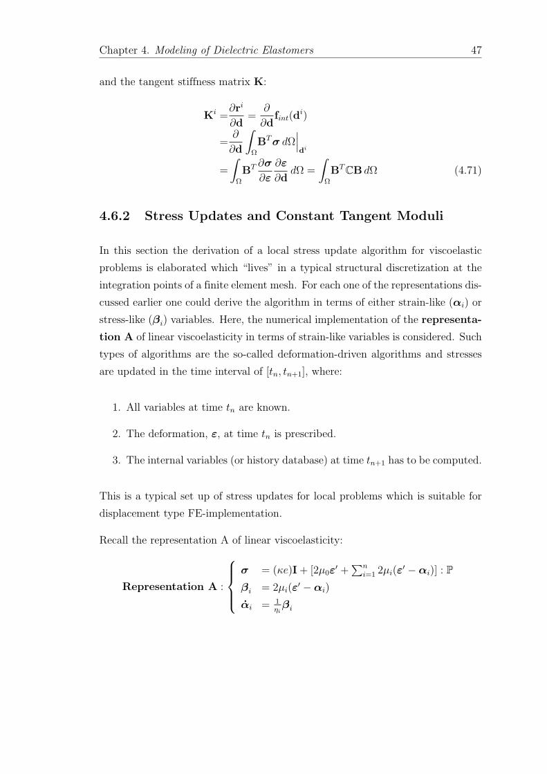
Chapter 4. Modeling of Dielectric Elastomers 47
and the tangent stiffness matrix K:
Ki =∂ri
∂d=
∂
∂dfint(d
i)
=∂
∂d
∫
Ω
BT σ dΩ∣∣∣di
=
∫
Ω
BT ∂σ
∂ε
∂ε
∂ddΩ =
∫
Ω
BTCB dΩ (4.71)
4.6.2 Stress Updates and Constant Tangent Moduli
In this section the derivation of a local stress update algorithm for viscoelastic
problems is elaborated which “lives” in a typical structural discretization at the
integration points of a finite element mesh. For each one of the representations dis-
cussed earlier one could derive the algorithm in terms of either strain-like (αi) or
stress-like (βi) variables. Here, the numerical implementation of the representa-
tion A of linear viscoelasticity in terms of strain-like variables is considered. Such
types of algorithms are the so-called deformation-driven algorithms and stresses
are updated in the time interval of [tn, tn+1], where:
1. All variables at time tn are known.
2. The deformation, ε, at time tn is prescribed.
3. The internal variables (or history database) at time tn+1 has to be computed.
This is a typical set up of stress updates for local problems which is suitable for
displacement type FE-implementation.
Recall the representation A of linear viscoelasticity:
Representation A :
σ = (κe)I + [2µ0ε′ +
∑n
i=12µi(ε
′ − αi)] : P
βi = 2µi(ε′ − αi)
αi = 1
ηi
βi
Chapter 4. Modeling of Dielectric Elastomers 48
In a first step the evolution equation, αi = 1
ηi
βi, is integrated using a fully implicit
backward Euler scheme, i.e. :
αin+1 =
αin+1 − αi
n
∆t
=⇒ αin+1 = αi
n + ∆t αin+1
= αin + ∆t
1
ηi
βin+1
= αin + ∆t
2µi
ηi
(ε′
n+1− αi
n+1)
= αin +
∆t
τi
(ε′
n+1− αi
n+1) (4.72)
where τi =ηi
2µi
is the relaxation time.
Eq. (4.72) is a linear equation in αin+1 due to the linear form of the considered
model. Solving this for αin+1 gives:
αin+1 =
αin + (∆t
τi
)ε′
n+1
1 + ∆tτi
(4.73)
with this at hand the algorithmic stresses read:
σn+1 = (κen+1)I + 2µ0ε′
n+1 +n∑
i=1
2µi
(
ε′
n+1 −αi
n + (∆tτi
)ε′
n+1
1 + ∆tτi
)
(4.74)
the tangent moduli consistent with the chosen integration schemes are given by:
Cn+1 = κI ⊗ I +
[
2µ0 +n∑
i=1
2µi
(
1 −∆tτi
1 + ∆tτi
)]
: P (4.75)
The abovementioned algorithm can now be summarized as follows:
1. Given is the database ε,H at time tn and current deformation εn+1 at
time tn + ∆t with H = αi, · · · , αn
2. Decompose strain into volumetric, en+1 := tr[εn+1] and isochoric parts,
ε′
n+1 := dev[εn+1]
3. Set the algorithmic parameters and update history variables:

Chapter 4. Modeling of Dielectric Elastomers 49
3.1 Set the algorithmic parameters as:
Ci1 :=
∆t
τi
; Ci2 := 1 −
∆tτi
1 + ∆tτi
=1
1 + Ci1
3.2 Update History variables:
αin+1 =
αin + (∆t
τi
)ε′
n+1
1 + ∆tτi
and store Hn+1 = αin+1, · · · , αn
n+1
4. Compute stresses:
σn+1 = (κen+1)I + 2µ0ε′
n+1 +n∑
i=1
2µi
(
ε′
n+1 −αi
n + (∆tτi
)ε′
n+1
1 + ∆tτi
)
5. Compute constant tangent moduli:
Cn+1 = κI ⊗ I +
[
2µ0 +n∑
i=1
2µi
(
1 −∆tτi
1 + ∆tτi
)]
: P
4.6.3 Addition of the Maxwell Stress in the Material Model
Using the abovementioned stress-update algorithm one ends up only with elastic
stresses. The Cauchy stress tensor of an activated DE, however, contains, in
addition, the components of Maxwell stresses. As such, it is assumed that the
Maxwell stresses can be regarded as initial stresses in the system. Elastic stresses
calculated thereafter using the aforementioned stress-update algorithm is simply
added to the pre-existing stress components which finally result in the complete
description of the stresses in the system.
4.6.4 Implementation of the Algorithm in ABAQUS
ABAQUS general FE code is used in the present study. The reason why ABAQUS
has been chosen is ABAQUS’s capability to tailor to one ’s specific analysis re-
quirements through the usage of “user subroutines”. A complete list of such
routines along with the usage, general interfaces and requirements can be found
in Ref. [71, 72].
Chapter 4. Modeling of Dielectric Elastomers 50
Developing such routines requires a basic knowledge of FORTRAN programming
language. In the present study three user subroutines have been exploited; The
first one of which is a user subroutine called “SDVINI” used to define and initial-
ize the history variables associated with the stress-update algorithm, the second
subroutine called “SIGINI” is used to initialize the stress tensor and “UMAT”
user subroutine is used to implement the stress-update algorithm of linear vis-
coelastic material model. The convergence of UMAT subroutine depends on the
definition of the Jacobian of the routine known as DDSDDE. It corresponds to
the constant tangent moduli as defined in Sec. 4.6.2. The Appendix A contains
the subroutines used in the present study.
Using such subroutines demands inclusion of specific ABAQUS “Keywords” in the
input file as following:
1. The Keywords to use the UMAT:
*MATERIAL, NAME = <USER>
*USER MATERIAL, CONST = <number of constants>
<constants>
2. The Keywords to use SDVINI:
*DEPVAR
<number of solution dependent variables>,
*INITIAL CONDITIONS,TYPE=SOLUTION,USER
3. The Keywords to use SIGINI:
*INITIAL CONDITIONS,TYPE=STRESS,USER
Chapter 5
Numerical Simulation of
Dielectric Elastomers
5.1 General overview
In this chapter the results of the FE simulation of actuation principles of a cir-
cular DE using ABAQUS FE code are presented. First the verification of the
developed user material subroutine for ABAQUS (UMAT), then the demonstra-
tion of a model problem for DEs are presented. The model problem is the one
discussed in Ref. [1]. The details regarding the model are found in the respective
section. The ultimate goal of introducing such a model problem is to develop a
benchmark using which, one is further able to examine the developed material
routine and observe the potential shortcomings. In this fashion the model is first
simulated using ABAQUS material library and then with the UMAT.
5.2 UMAT Verification
How a UMAT was developed and further verified is presented in this section. It
was first attempted to implement the previously mentioned stress-update algo-
rithm of linear viscoelasticity (representation A) in ABAQUS as a user material
subroutine (UMAT). This UMAT is presented in Appendix A. The verification
51
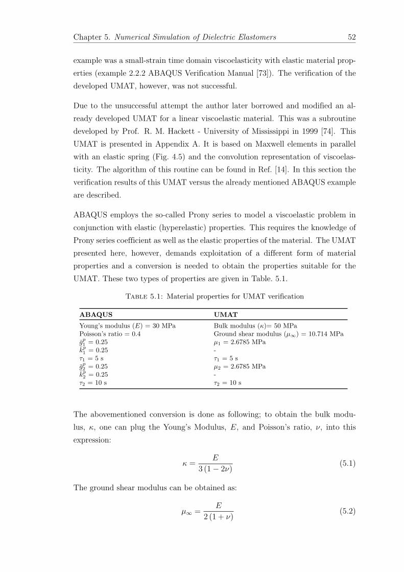
Chapter 5. Numerical Simulation of Dielectric Elastomers 52
example was a small-strain time domain viscoelasticity with elastic material prop-
erties (example 2.2.2 ABAQUS Verification Manual [73]). The verification of the
developed UMAT, however, was not successful.
Due to the unsuccessful attempt the author later borrowed and modified an al-
ready developed UMAT for a linear viscoelastic material. This was a subroutine
developed by Prof. R. M. Hackett - University of Mississippi in 1999 [74]. This
UMAT is presented in Appendix A. It is based on Maxwell elements in parallel
with an elastic spring (Fig. 4.5) and the convolution representation of viscoelas-
ticity. The algorithm of this routine can be found in Ref. [14]. In this section the
verification results of this UMAT versus the already mentioned ABAQUS example
are described.
ABAQUS employs the so-called Prony series to model a viscoelastic problem in
conjunction with elastic (hyperelastic) properties. This requires the knowledge of
Prony series coefficient as well as the elastic properties of the material. The UMAT
presented here, however, demands exploitation of a different form of material
properties and a conversion is needed to obtain the properties suitable for the
UMAT. These two types of properties are given in Table. 5.1.
Table 5.1: Material properties for UMAT verification
ABAQUS UMAT
Young’s modulus (E) = 30 MPa Bulk modulus (κ)= 50 MPaPoisson’s ratio = 0.4 Ground shear modulus (µ∞) = 10.714 MPag
p
1= 0.25 µ1 = 2.6785 MPa
kp
1= 0.25 -
τ1 = 5 s τ1 = 5 sg
p
2= 0.25 µ2 = 2.6785 MPa
kp
2= 0.25 -
τ2 = 10 s τ2 = 10 s
The abovementioned conversion is done as following; to obtain the bulk modu-
lus, κ, one can plug the Young’s Modulus, E, and Poisson’s ratio, ν, into this
expression:
κ =E
3 (1 − 2ν)(5.1)
The ground shear modulus can be obtained as:
µ∞ =E
2 (1 + ν)(5.2)
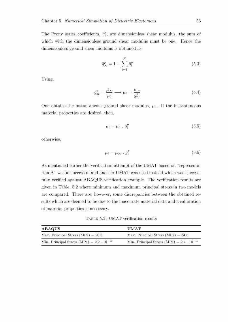
Chapter 5. Numerical Simulation of Dielectric Elastomers 53
The Prony series coefficients, gpi , are dimensionless shear modulus, the sum of
which with the dimensionless ground shear modulus must be one. Hence the
dimensionless ground shear modulus is obtained as:
gp∞
= 1 −
N∑
i=1
gpi (5.3)
Using,
gp∞
=µ∞
µ0
−→ µ0 =µ∞
gp∞
(5.4)
One obtains the instantaneous ground shear modulus, µ0. If the instantaneous
material properties are desired, then,
µi = µ0 . gpi (5.5)
otherwise,
µi = µ∞ . gpi (5.6)
As mentioned earlier the verification attempt of the UMAT based on “representa-
tion A” was unsuccessful and another UMAT was used instead which was success-
fully verified against ABAQUS verification example. The verification results are
given in Table. 5.2 where minimum and maximum principal stress in two models
are compared. There are, however, some discrepancies between the obtained re-
sults which are deemed to be due to the inaccurate material data and a calibration
of material properties is necessary.
Table 5.2: UMAT verification results
ABAQUS UMAT
Max. Principal Stress (MPa) = 20.8 Max. Principal Stress (MPa) = 34.5
Min. Principal Stress (MPa) = 2.2 . 10−10 Min. Principal Stress (MPa) = 2.4 . 10−10
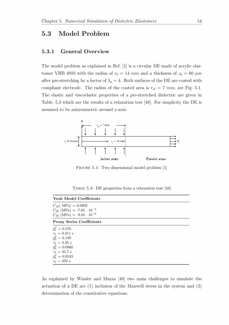
Chapter 5. Numerical Simulation of Dielectric Elastomers 54
5.3 Model Problem
5.3.1 General Overview
The model problem as explained in Ref. [1] is a circular DE made of acrylic elas-
tomer VHB 4910 with the radius of r0 = 14 mm and a thickness of z0 = 60 µm
after pre-stretching by a factor of λp = 4. Both surfaces of the DE are coated with
compliant electrode. The radius of the coated area is rel = 7 mm, see Fig. 5.1.
The elastic and viscoelastic properties of a pre-stretched dielectric are given in
Table. 5.3 which are the results of a relaxation test [48]. For simplicity the DE is
assumed to be axisymmetric around y-axis.
Figure 5.1: Two dimensional model problem [1]
Table 5.3: DE properties from a relaxation test [48]
Yeoh Model Coefficients
C10( MPa) = 0.0803C20 (MPa) = -7.65 . 10−4
C30 (MPa) = 9.84 . 10−6
Prony Series Coefficients
gp
1= 0.570
τ1 = 0.311 sg
p
2= 0.189
τ2 = 3.35 sg
p
3= 0.0860
τ3 = 35.7 sg
p
4= 0.0543
τ4 = 370 s
As explained by Wissler and Mazza [48] two main challenges to simulate the
actuation of a DE are (1) inclusion of the Maxwell stress in the system and (2)
determination of the constitutive equations.
Chapter 5. Numerical Simulation of Dielectric Elastomers 55
To address the first difficulty two approaches was employed to include the Maxwell
stress in the system. In the first approach the Maxwell stress was applied through
a lateral pressure (pr) along with the tractions on both sides of the DE. The
Maxwell stress was computed according to Eq. 4.52 and was then applied as a
uniform pressure on the lateral surfaces of the DE. The tractions were computed
using Eq. 4.53 and then applied as uniform pressures on the electrode surfaces.
In the second approach, the Maxwell stress was assumed as a residual stress (pre-
stress) in the system and was applied using an ABAQUS user subroutine called
“SIGINI”. The way the tractions were enforced in the system remained unchanged
in this approach.
Either approaches used the current thickness of the DE to compute the Maxwell
stress. As such, one had to know the stretch ratio in the thickness direction (λt1)
to get the current thickness. As stated in Ref. [48], one expects 10% ≈ 30%
increase in length (elongation) when the DEs is activated. Since the stretch ratio
in the thickness direction was unknown, a series of trials were run to calibrate the
amount of stretch ratio which gave the 10% ≈ 30% elongation upon activation of
the DE.
Another aspect which is discussed in this section is the usage of ABAQUS mate-
rial library versus the developed UMAT. A hyper-viscoelastic material model was
used from ABAQUS material library. The hyperelastic part was based on Yeoh
hyperelastic model [52] and the viscoelastic part was based on the time domain
Prony series. The results obtained with the ABAQUS material library was used
as a benchmark to determine if the developed UMAT was accurate enough for the
sake of simulation.
In the following sections, first a series of trials was carried out to find the stretch
ratio of the DE. After obtaining the stretch ratio three cases were tested with only
tractions, lateral pressure/pre-stress and both tractions and lateral pressure/pre-
stress in the system. The effect of applied voltage on the actuation of DEs was
further investigated. Finally a comparison was made between the UMAT and
ABAQUS material library.
1The ratio between the thickness in the current configuration, z0, and the thickness in thereference configuration, z.
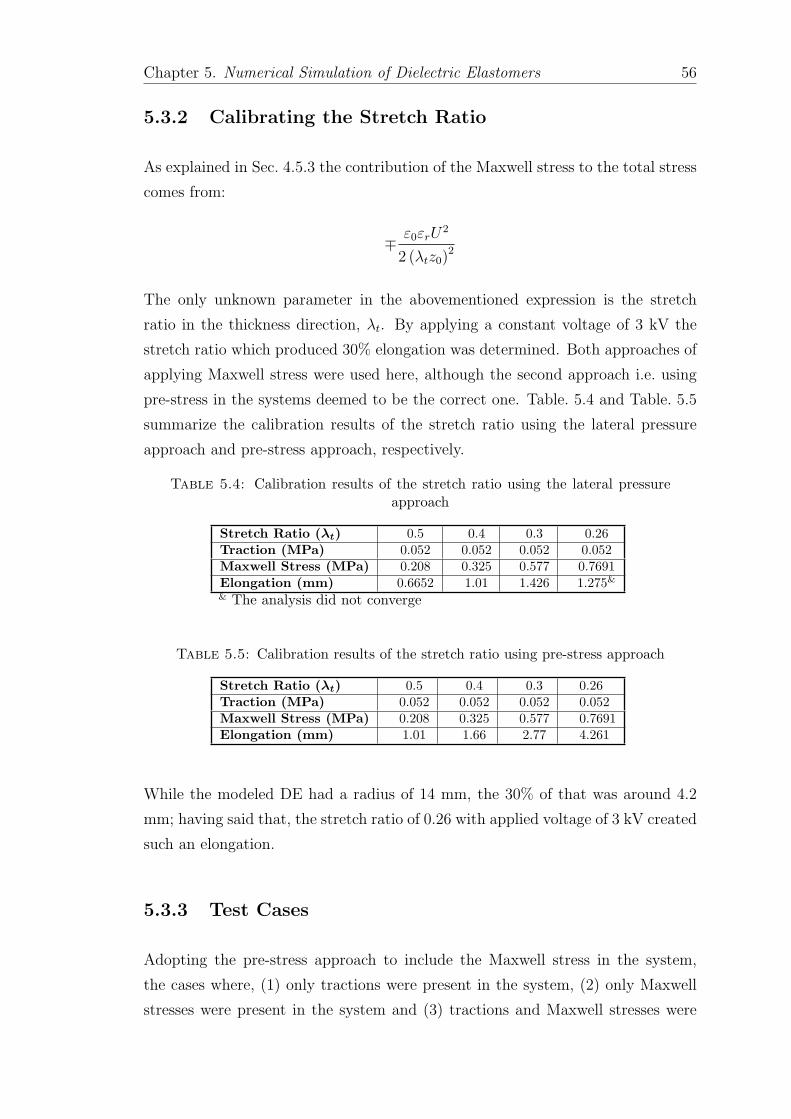
Chapter 5. Numerical Simulation of Dielectric Elastomers 56
5.3.2 Calibrating the Stretch Ratio
As explained in Sec. 4.5.3 the contribution of the Maxwell stress to the total stress
comes from:
∓ε0εrU
2
2 (λtz0)2
The only unknown parameter in the abovementioned expression is the stretch
ratio in the thickness direction, λt. By applying a constant voltage of 3 kV the
stretch ratio which produced 30% elongation was determined. Both approaches of
applying Maxwell stress were used here, although the second approach i.e. using
pre-stress in the systems deemed to be the correct one. Table. 5.4 and Table. 5.5
summarize the calibration results of the stretch ratio using the lateral pressure
approach and pre-stress approach, respectively.
Table 5.4: Calibration results of the stretch ratio using the lateral pressureapproach
Stretch Ratio (λt) 0.5 0.4 0.3 0.26Traction (MPa) 0.052 0.052 0.052 0.052Maxwell Stress (MPa) 0.208 0.325 0.577 0.7691Elongation (mm) 0.6652 1.01 1.426 1.275&
& The analysis did not converge
Table 5.5: Calibration results of the stretch ratio using pre-stress approach
Stretch Ratio (λt) 0.5 0.4 0.3 0.26Traction (MPa) 0.052 0.052 0.052 0.052Maxwell Stress (MPa) 0.208 0.325 0.577 0.7691Elongation (mm) 1.01 1.66 2.77 4.261
While the modeled DE had a radius of 14 mm, the 30% of that was around 4.2
mm; having said that, the stretch ratio of 0.26 with applied voltage of 3 kV created
such an elongation.
5.3.3 Test Cases
Adopting the pre-stress approach to include the Maxwell stress in the system,
the cases where, (1) only tractions were present in the system, (2) only Maxwell
stresses were present in the system and (3) tractions and Maxwell stresses were
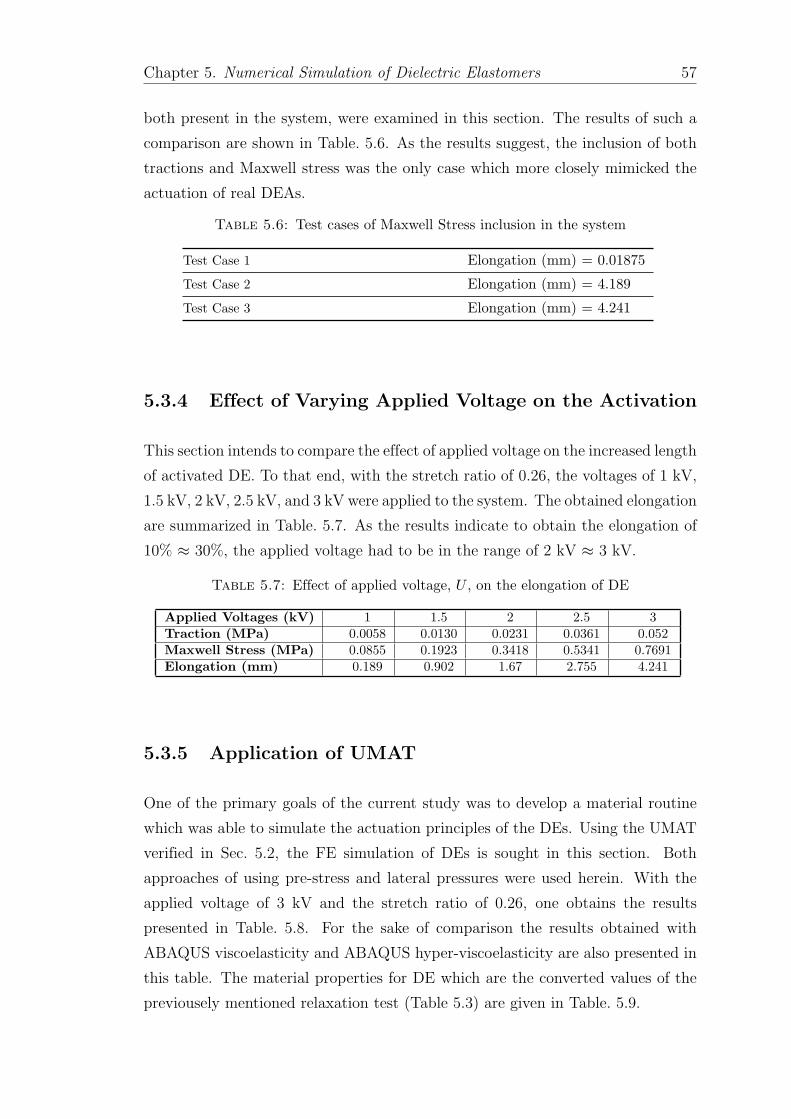
Chapter 5. Numerical Simulation of Dielectric Elastomers 57
both present in the system, were examined in this section. The results of such a
comparison are shown in Table. 5.6. As the results suggest, the inclusion of both
tractions and Maxwell stress was the only case which more closely mimicked the
actuation of real DEAs.
Table 5.6: Test cases of Maxwell Stress inclusion in the system
Test Case 1 Elongation (mm) = 0.01875
Test Case 2 Elongation (mm) = 4.189
Test Case 3 Elongation (mm) = 4.241
5.3.4 Effect of Varying Applied Voltage on the Activation
This section intends to compare the effect of applied voltage on the increased length
of activated DE. To that end, with the stretch ratio of 0.26, the voltages of 1 kV,
1.5 kV, 2 kV, 2.5 kV, and 3 kV were applied to the system. The obtained elongation
are summarized in Table. 5.7. As the results indicate to obtain the elongation of
10% ≈ 30%, the applied voltage had to be in the range of 2 kV ≈ 3 kV.
Table 5.7: Effect of applied voltage, U , on the elongation of DE
Applied Voltages (kV) 1 1.5 2 2.5 3Traction (MPa) 0.0058 0.0130 0.0231 0.0361 0.052Maxwell Stress (MPa) 0.0855 0.1923 0.3418 0.5341 0.7691Elongation (mm) 0.189 0.902 1.67 2.755 4.241
5.3.5 Application of UMAT
One of the primary goals of the current study was to develop a material routine
which was able to simulate the actuation principles of the DEs. Using the UMAT
verified in Sec. 5.2, the FE simulation of DEs is sought in this section. Both
approaches of using pre-stress and lateral pressures were used herein. With the
applied voltage of 3 kV and the stretch ratio of 0.26, one obtains the results
presented in Table. 5.8. For the sake of comparison the results obtained with
ABAQUS viscoelasticity and ABAQUS hyper-viscoelasticity are also presented in
this table. The material properties for DE which are the converted values of the
previousely mentioned relaxation test (Table 5.3) are given in Table. 5.9.
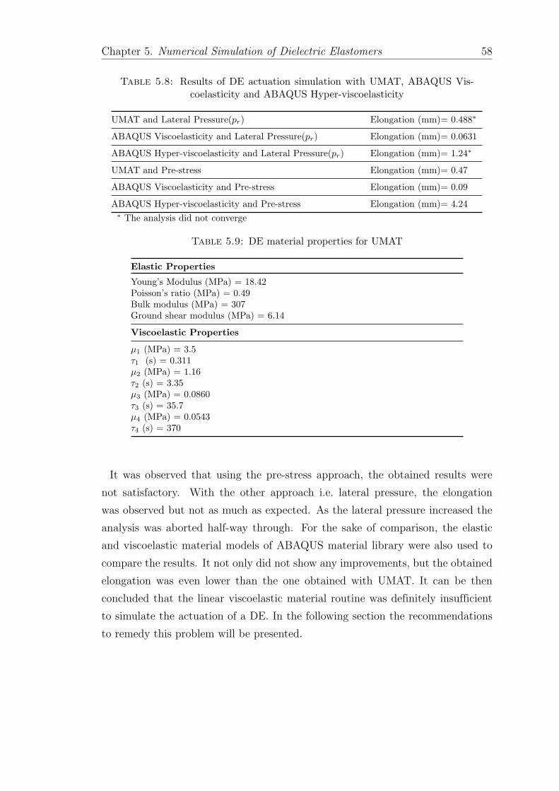
Chapter 5. Numerical Simulation of Dielectric Elastomers 58
Table 5.8: Results of DE actuation simulation with UMAT, ABAQUS Vis-coelasticity and ABAQUS Hyper-viscoelasticity
UMAT and Lateral Pressure(pr) Elongation (mm)= 0.488∗
ABAQUS Viscoelasticity and Lateral Pressure(pr) Elongation (mm)= 0.0631
ABAQUS Hyper-viscoelasticity and Lateral Pressure(pr) Elongation (mm)= 1.24∗
UMAT and Pre-stress Elongation (mm)= 0.47
ABAQUS Viscoelasticity and Pre-stress Elongation (mm)= 0.09
ABAQUS Hyper-viscoelasticity and Pre-stress Elongation (mm)= 4.24∗ The analysis did not converge
Table 5.9: DE material properties for UMAT
Elastic Properties
Young’s Modulus (MPa) = 18.42Poisson’s ratio (MPa) = 0.49Bulk modulus (MPa) = 307Ground shear modulus (MPa) = 6.14
Viscoelastic Properties
µ1 (MPa) = 3.5τ1 (s) = 0.311µ2 (MPa) = 1.16τ2 (s) = 3.35µ3 (MPa) = 0.0860τ3 (s) = 35.7µ4 (MPa) = 0.0543τ4 (s) = 370
It was observed that using the pre-stress approach, the obtained results were
not satisfactory. With the other approach i.e. lateral pressure, the elongation
was observed but not as much as expected. As the lateral pressure increased the
analysis was aborted half-way through. For the sake of comparison, the elastic
and viscoelastic material models of ABAQUS material library were also used to
compare the results. It not only did not show any improvements, but the obtained
elongation was even lower than the one obtained with UMAT. It can be then
concluded that the linear viscoelastic material routine was definitely insufficient
to simulate the actuation of a DE. In the following section the recommendations
to remedy this problem will be presented.

Chapter 5. Numerical Simulation of Dielectric Elastomers 59
5.3.6 Three Dimensional Extension
In this section the three dimensional extension of the model problem with the
same geometry data and material properties will be presented, see Fig. 5.2.
ZT
R
Z
Y
X
X
Y
Z
Figure 5.2: Three dimensional model problem
For this model the Maxwell stress was included using the pre-stress approach.
Assuming the stretch ratio of λt = 0.26, the actuation was simulated with the
applied voltages of 2 kV, 2.5 kV, and 3 kV. The resulting tractions and stresses
were those given in Table. 5.7.
The ABAQUS material library was used to run the simulation. The activated DE
with 3 kV applied voltage is illustrated in Fig. 5.3.
Table. 5.10 presents the obtained results for actuation simulation of DE using both
ABAQUS material library. For comparison, the 2D results are also presented in
this table.
Table 5.10: Results of 3D DE actuation simulation
Applied Voltage U (kV) 3D Elongation(mm) 2D Elongation(mm)
2 0.9714 1.67
2.5 1.482 2.76
3 2.069 4.24
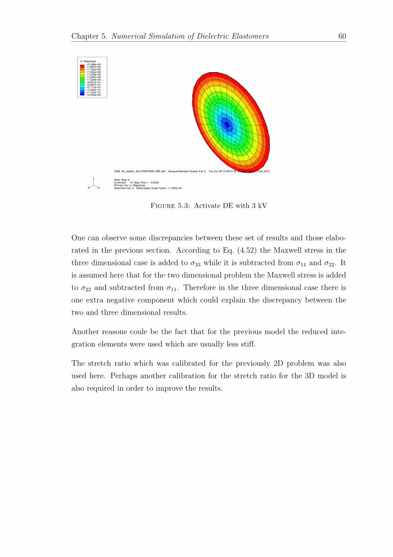
Chapter 5. Numerical Simulation of Dielectric Elastomers 60
U, Magnitude
+0.000e+00+1.724e−01+3.449e−01+5.173e−01+6.897e−01+8.621e−01+1.035e+00+1.207e+00+1.379e+00+1.552e+00+1.724e+00+1.897e+00+2.069e+00
Step: Step−2Increment 10: Step Time = 0.6438Primary Var: U, MagnitudeDeformed Var: U Deformation Scale Factor: +1.000e+00
ODB: 3D_wissler_3kV1276079561.856.odb Abaqus/Standard Version 6.8−2 Tue Jun 08 10:46:21 W. Europe Daylight Time 2010
X
Y
Z
Figure 5.3: Activate DE with 3 kV
One can observe some discrepancies between these set of results and those elabo-
rated in the previous section. According to Eq. (4.52) the Maxwell stress in the
three dimensional case is added to σ33 while it is subtracted from σ11 and σ22. It
is assumed here that for the two dimensional problem the Maxwell stress is added
to σ22 and subtracted from σ11. Therefore in the three dimensional case there is
one extra negative component which could explain the discrepancy between the
two and three dimensional results.
Another reasone coule be the fact that for the previous model the reduced inte-
gration elements were used which are usually less stiff.
The stretch ratio which was calibrated for the previously 2D problem was also
used here. Perhaps another calibration for the stretch ratio for the 3D model is
also required in order to improve the results.
Chapter 6
Conclusion and Outlook
The objective of the current study was to investigate the viscoelastic behavior of
DEAs using the Finite Element Method. To that end a linear viscoelastic material
routine was implemented in ABAQUS Finite Element code as a user subroutine.
To account for the stresses induced by the electric field, the stress tensor was
initiated with some pre-stresses based on the work of Goulbourne et al. [6].
Two model problems were introduced to be served as a benchmark to verify the
results obtained with the linear viscoelastic material model. The visco-hyperelastic
material model was exploited for these two models. It was then concluded that:
• The linear viscoelastic material model was insufficient to correctly simulate
the actuation of DE.
• To obtain the elongation of 10% ≈ 30%, the applied voltage must be in the
range of 2 kV ≈ 3 kV.
• To correctly simulate the actuation of DE one should consider both tractions
on the surfaces of DE and the Maxwell stresses induced by electric field.
• To find the correct value of Maxwell stress one should know the correct
stretch ratio in the direction of applied voltage.
Based on the obtained results the following set of actions are recommended:
• To further enhance the simulation of DEs and obtain a more realistic result,
the use of hyperelastic material model is recommended.
61
Chapter 6. Conclusion and Outlook 62
• It is also suggested to implement the material routine with the Maxwell
stresses included in the routine as the electric free term similar to the work
of Zhao and Suo [2].
• For the current work the radial DEs were used. Simulation of other configurations
is recommended.
• Conducting a parametric study is also suggested proceeded by an optimiza-
tion to find the optimal configuration of DEs. Needless to say, one should
decide on the proper design variables, objective function and constraints
prior to setting up the optimization problem.
Appendix A
User Subroutines
A.1 UMAT for Representation A
The following subroutine is the modified version of a routine originally written in
C++. It was developed at the Institute of Applied Mechanics (Chair I), univer-
sity of Stuttgart to be used in conjunction with FEAPpv finite element program.
FEAPpv is a general purpose finile element analysis program designed for re-
search and educational use by Robert L. Taylor. The source code and manuals for
FEAPpv are available at http://www.ce.berkeley.edu/projects/feap/feappv.
The program is described in Ref. [65]. As mentioned in chapter four, it has been
developed for linear viscoelasticity in terms of internal variable. The correspond-
ing generalized Maxwell model consists of two Maxwell elements in parallel with
an elastic spring (N = 2).
C *********************************************************************
SUBROUTINE SDVINI(STATEV,COORDS,NSTATV,NCRDS,NOEL,NPT,LAYER,KSPT)
C
INCLUDE ’ABA_PARAM.INC’
C
DIMENSION STATEV(NSTATV),COORDS(NCRDS)
INTEGER I
C
DO I=1,NSTATV
STATEV(I)=0.0D0
63
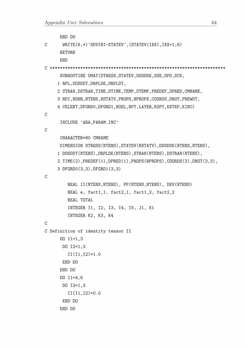
Appendix User Subroutines 64
END DO
C WRITE(6,*)’SDVINI-STATEV’,(STATEV(IXX),IXX=1,6)
RETURN
END
C *********************************************************************
SUBROUTINE UMAT(STRESS,STATEV,DDSDDE,SSE,SPD,SCD,
1 RPL,DDSDDT,DRPLDE,DRPLDT,
2 STRAN,DSTRAN,TIME,DTIME,TEMP,DTEMP,PREDEF,DPRED,CMNAME,
3 NDI,NSHR,NTENS,NSTATV,PROPS,NPROPS,COORDS,DROT,PNEWDT,
4 CELENT,DFGRD0,DFGRD1,NOEL,NPT,LAYER,KSPT,KSTEP,KINC)
C
INCLUDE ’ABA_PARAM.INC’
C
CHARACTER*80 CMNAME
DIMENSION STRESS(NTENS),STATEV(NSTATV),DDSDDE(NTENS,NTENS),
1 DDSDDT(NTENS),DRPLDE(NTENS),STRAN(NTENS),DSTRAN(NTENS),
2 TIME(2),PREDEF(1),DPRED(1),PROPS(NPROPS),COORDS(3),DROT(3,3),
3 DFGRD0(3,3),DFGRD1(3,3)
C
REAL II(NTENS,NTENS), PP(NTENS,NTENS), DEV(NTENS)
REAL e, fact1_1, fact2_1, fact1_2, fact2_2
REAL TOTAL
INTEGER I1, I2, I3, I4, I5, J1, K1
INTEGER K2, K3, K4
C
C Definition of identity tensor II
DO I1=1,3
DO I2=1,3
II(I1,I2)=1.0
END DO
END DO
DO I1=4,6
DO I2=1,3
II(I1,I2)=0.0
END DO
END DO
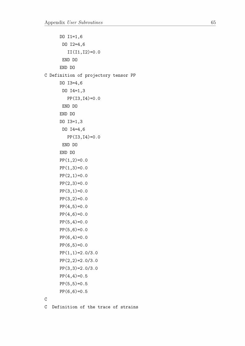
Appendix User Subroutines 65
DO I1=1,6
DO I2=4,6
II(I1,I2)=0.0
END DO
END DO
C Definition of projectory tensor PP
DO I3=4,6
DO I4=1,3
PP(I3,I4)=0.0
END DO
END DO
DO I3=1,3
DO I4=4,6
PP(I3,I4)=0.0
END DO
END DO
PP(1,2)=0.0
PP(1,3)=0.0
PP(2,1)=0.0
PP(2,3)=0.0
PP(3,1)=0.0
PP(3,2)=0.0
PP(4,5)=0.0
PP(4,6)=0.0
PP(5,4)=0.0
PP(5,6)=0.0
PP(6,4)=0.0
PP(6,5)=0.0
PP(1,1)=2.0/3.0
PP(2,2)=2.0/3.0
PP(3,3)=2.0/3.0
PP(4,4)=0.5
PP(5,5)=0.5
PP(6,6)=0.5
C
C Definition of the trace of strains
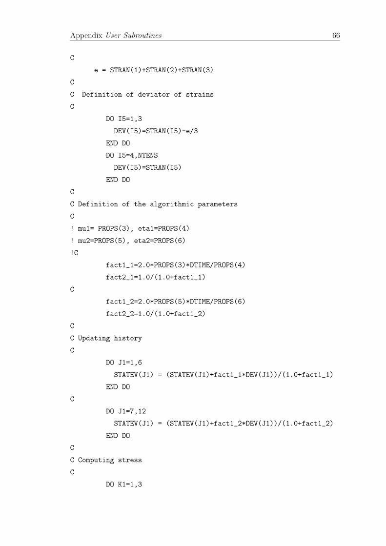
Appendix User Subroutines 66
C
e = STRAN(1)+STRAN(2)+STRAN(3)
C
C Definition of deviator of strains
C
DO I5=1,3
DEV(I5)=STRAN(I5)-e/3
END DO
DO I5=4,NTENS
DEV(I5)=STRAN(I5)
END DO
C
C Definition of the algorithmic parameters
C
! mu1= PROPS(3), eta1=PROPS(4)
! mu2=PROPS(5), eta2=PROPS(6)
!C
fact1_1=2.0*PROPS(3)*DTIME/PROPS(4)
fact2_1=1.0/(1.0+fact1_1)
C
fact1_2=2.0*PROPS(5)*DTIME/PROPS(6)
fact2_2=1.0/(1.0+fact1_2)
C
C Updating history
C
DO J1=1,6
STATEV(J1) = (STATEV(J1)+fact1_1*DEV(J1))/(1.0+fact1_1)
END DO
C
DO J1=7,12
STATEV(J1) = (STATEV(J1)+fact1_2*DEV(J1))/(1.0+fact1_2)
END DO
C
C Computing stress
C
DO K1=1,3
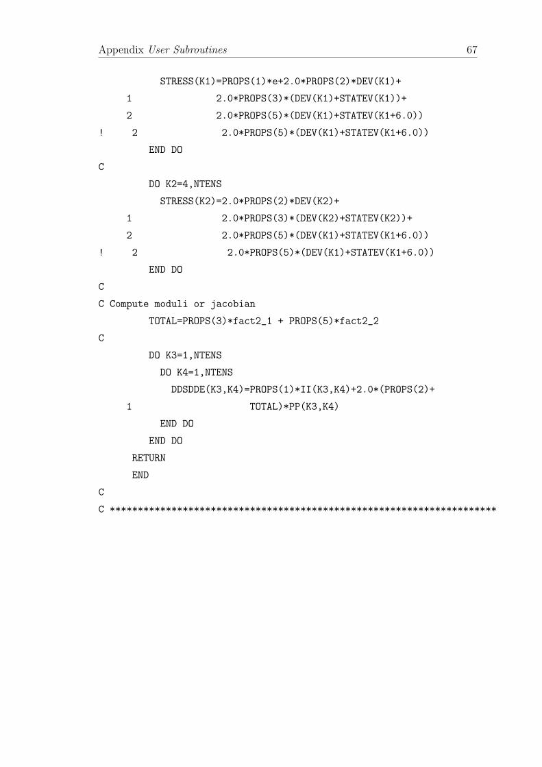
Appendix User Subroutines 67
STRESS(K1)=PROPS(1)*e+2.0*PROPS(2)*DEV(K1)+
1 2.0*PROPS(3)*(DEV(K1)+STATEV(K1))+
2 2.0*PROPS(5)*(DEV(K1)+STATEV(K1+6.0))
! 2 2.0*PROPS(5)*(DEV(K1)+STATEV(K1+6.0))
END DO
C
DO K2=4,NTENS
STRESS(K2)=2.0*PROPS(2)*DEV(K2)+
1 2.0*PROPS(3)*(DEV(K2)+STATEV(K2))+
2 2.0*PROPS(5)*(DEV(K1)+STATEV(K1+6.0))
! 2 2.0*PROPS(5)*(DEV(K1)+STATEV(K1+6.0))
END DO
C
C Compute moduli or jacobian
TOTAL=PROPS(3)*fact2_1 + PROPS(5)*fact2_2
C
DO K3=1,NTENS
DO K4=1,NTENS
DDSDDE(K3,K4)=PROPS(1)*II(K3,K4)+2.0*(PROPS(2)+
1 TOTAL)*PP(K3,K4)
END DO
END DO
RETURN
END
C
C *********************************************************************
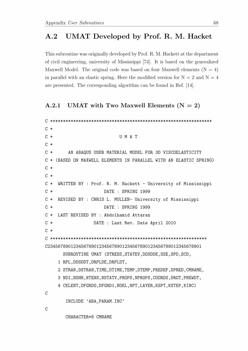
Appendix User Subroutines 68
A.2 UMAT Developed by Prof. R. M. Hacket
This subroutine was originally developed by Prof. R. M. Hackett at the department
of civil engineering, university of Mississippi [74]. It is based on the generalized
Maxwell Model. The original code was based on four Maxwell elements (N = 4)
in parallel with an elastic spring. Here the modified version for N = 2 and N = 4
are presented. The corresponding algorithm can be found in Ref. [14].
A.2.1 UMAT with Two Maxwell Elements (N = 2)
C ***************************************************************
C *
C * U M A T
C *
C * AN ABAQUS USER MATERIAL MODEL FOR 3D VISCOELASTICITY
C * (BASED ON MAXWELL ELEMENTS IN PARALLEL WITH AN ELASTIC SPRING)
C *
C *
C * WRITTEN BY : Prof. R. M. Hackett - University of Mississippi
C * DATE : SPRING 1999
C * REVISED BY : CHRIS L. MULLEN- University of Mississippi
C * DATE : SPRING 1999
C * LAST REVISED BY : Abdolhamid Attaran
C * DATE : Last Rev. Date April 2010
C *
C *************************************************************
C234567890123456789012345678901234567890123456789012345678901
SUBROUTINE UMAT (STRESS,STATEV,DDSDDE,SSE,SPD,SCD,
1 RPL,DDSDDT,DRPLDE,DRPLDT,
2 STRAN,DSTRAN,TIME,DTIME,TEMP,DTEMP,PREDEF,DPRED,CMNAME,
3 NDI,NSHR,NTENS,NSTATV,PROPS,NPROPS,COORDS,DROT,PNEWDT,
4 CELENT,DFGRDO,DFGRD1,NOEL,NPT,LAYER,KSPT,KSTEP,KINC)
C
INCLUDE ’ABA_PARAM.INC’
C
CHARACTER*8 CMNAME
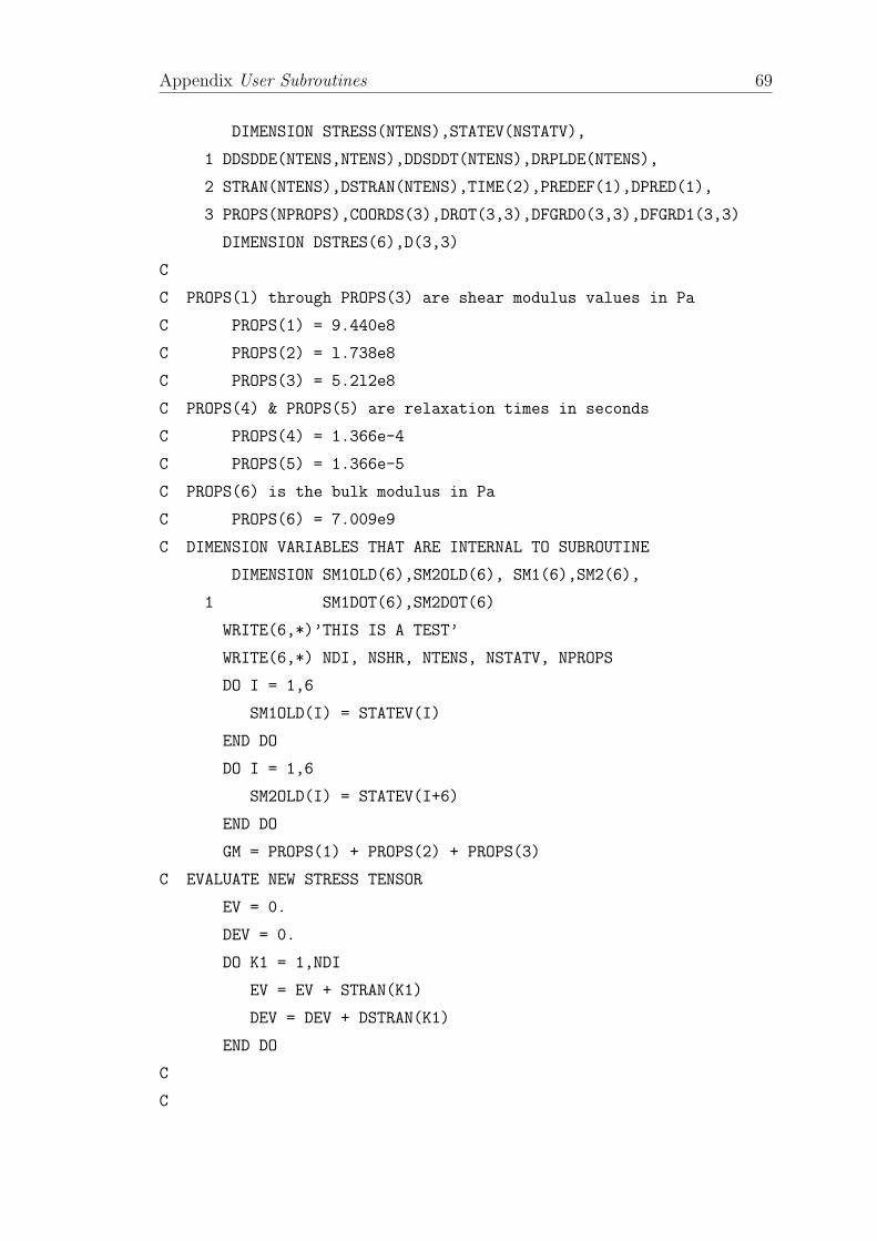
Appendix User Subroutines 69
DIMENSION STRESS(NTENS),STATEV(NSTATV),
1 DDSDDE(NTENS,NTENS),DDSDDT(NTENS),DRPLDE(NTENS),
2 STRAN(NTENS),DSTRAN(NTENS),TIME(2),PREDEF(1),DPRED(1),
3 PROPS(NPROPS),COORDS(3),DROT(3,3),DFGRD0(3,3),DFGRD1(3,3)
DIMENSION DSTRES(6),D(3,3)
C
C PROPS(l) through PROPS(3) are shear modulus values in Pa
C PROPS(1) = 9.440e8
C PROPS(2) = l.738e8
C PROPS(3) = 5.2l2e8
C PROPS(4) & PROPS(5) are relaxation times in seconds
C PROPS(4) = 1.366e-4
C PROPS(5) = 1.366e-5
C PROPS(6) is the bulk modulus in Pa
C PROPS(6) = 7.009e9
C DIMENSION VARIABLES THAT ARE INTERNAL TO SUBROUTINE
DIMENSION SM1OLD(6),SM2OLD(6), SM1(6),SM2(6),
1 SM1DOT(6),SM2DOT(6)
WRITE(6,*)’THIS IS A TEST’
WRITE(6,*) NDI, NSHR, NTENS, NSTATV, NPROPS
DO I = 1,6
SM1OLD(I) = STATEV(I)
END DO
DO I = 1,6
SM2OLD(I) = STATEV(I+6)
END DO
GM = PROPS(1) + PROPS(2) + PROPS(3)
C EVALUATE NEW STRESS TENSOR
EV = 0.
DEV = 0.
DO K1 = 1,NDI
EV = EV + STRAN(K1)
DEV = DEV + DSTRAN(K1)
END DO
C
C
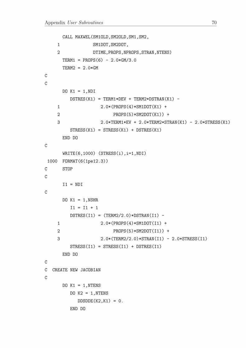
Appendix User Subroutines 70
CALL MAXWEL(SM1OLD,SM2OLD,SM1,SM2,
1 SM1DOT,SM2DOT,
2 DTIME,PROPS,NPROPS,STRAN,NTENS)
TERM1 = PROPS(6) - 2.0*GM/3.0
TERM2 = 2.0*GM
C
C
DO K1 = 1,NDI
DSTRES(K1) = TERM1*DEV + TERM2*DSTRAN(K1) -
1 2.0*(PROPS(4)*SM1DOT(K1) +
2 PROPS(5)*SM2DOT(K1)) +
3 2.0*TERM1*EV + 2.0*TERM2*STRAN(K1) - 2.0*STRESS(K1)
STRESS(K1) = STRESS(K1) + DSTRES(K1)
END DO
C
WRITE(6,1000) (STRESS(i),i=1,NDI)
1000 FORMAT(6(1pe12.3))
C STOP
C
I1 = NDI
C
DO K1 = 1,NSHR
I1 = I1 + 1
DSTRES(I1) = (TERM2/2.0)*DSTRAN(I1) -
1 2.0*(PROPS(4)*SM1DOT(I1) +
2 PROPS(5)*SM2DOT(I1)) +
3 2.0*(TERM2/2.0)*STRAN(I1) - 2.0*STRESS(I1)
STRESS(I1) = STRESS(I1) + DSTRES(I1)
END DO
C
C CREATE NEW JACOBIAN
C
DO K1 = 1,NTENS
DO K2 = 1,NTENS
DDSDDE(K2,K1) = 0.
END DO
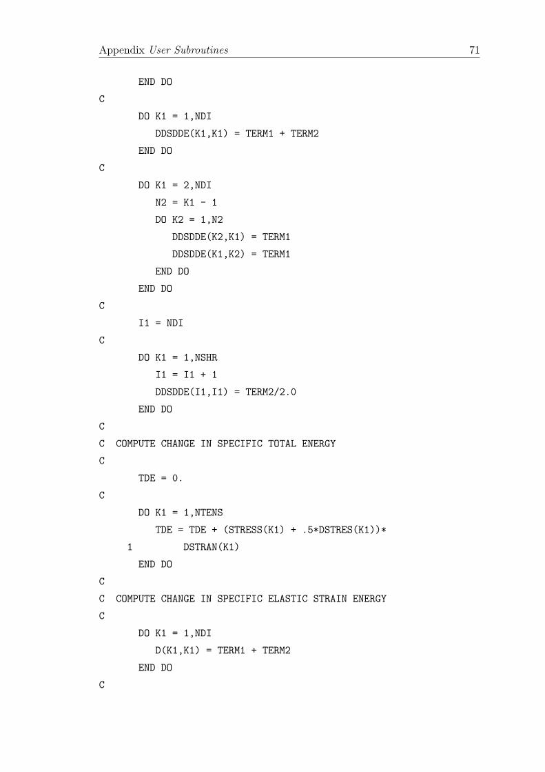
Appendix User Subroutines 71
END DO
C
DO K1 = 1,NDI
DDSDDE(K1,K1) = TERM1 + TERM2
END DO
C
DO K1 = 2,NDI
N2 = K1 - 1
DO K2 = 1,N2
DDSDDE(K2,K1) = TERM1
DDSDDE(K1,K2) = TERM1
END DO
END DO
C
I1 = NDI
C
DO K1 = 1,NSHR
I1 = I1 + 1
DDSDDE(I1,I1) = TERM2/2.0
END DO
C
C COMPUTE CHANGE IN SPECIFIC TOTAL ENERGY
C
TDE = 0.
C
DO K1 = 1,NTENS
TDE = TDE + (STRESS(K1) + .5*DSTRES(K1))*
1 DSTRAN(K1)
END DO
C
C COMPUTE CHANGE IN SPECIFIC ELASTIC STRAIN ENERGY
C
DO K1 = 1,NDI
D(K1,K1) = TERM1 + TERM2
END DO
C
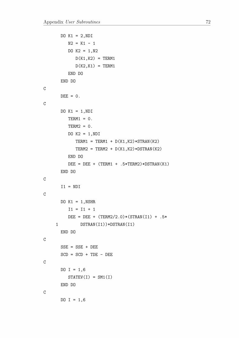
Appendix User Subroutines 72
DO K1 = 2,NDI
N2 = K1 - 1
DO K2 = 1,N2
D(K1,K2) = TERM1
D(K2,K1) = TERM1
END DO
END DO
C
DEE = 0.
C
DO K1 = 1,NDI
TERM1 = 0.
TERM2 = 0.
DO K2 = 1,NDI
TERM1 = TERM1 + D(K1,K2)*STRAN(K2)
TERM2 = TERM2 + D(K1,K2)*DSTRAN(K2)
END DO
DEE = DEE + (TERM1 + .5*TERM2)*DSTRAN(K1)
END DO
C
I1 = NDI
C
DO K1 = 1,NSHR
I1 = I1 + 1
DEE = DEE + (TERM2/2.0)*(STRAN(I1) + .5*
1 DSTRAN(I1))*DSTRAN(I1)
END DO
C
SSE = SSE + DEE
SCD = SCD + TDE - DEE
C
DO I = 1,6
STATEV(I) = SM1(I)
END DO
C
DO I = 1,6
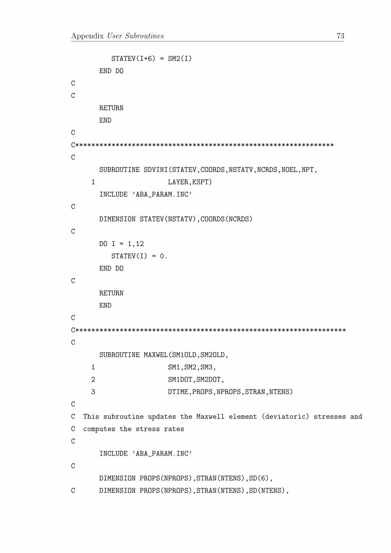
Appendix User Subroutines 73
STATEV(I+6) = SM2(I)
END DO
C
C
RETURN
END
C
C****************************************************************
C
SUBROUTINE SDVINI(STATEV,COORDS,NSTATV,NCRDS,NOEL,NPT,
1 LAYER,KSPT)
INCLUDE ’ABA_PARAM.INC’
C
DIMENSION STATEV(NSTATV),COORDS(NCRDS)
C
DO I = 1,12
STATEV(I) = 0.
END DO
C
RETURN
END
C
C*******************************************************************
C
SUBROUTINE MAXWEL(SM1OLD,SM2OLD,
1 SM1,SM2,SM3,
2 SM1DOT,SM2DOT,
3 DTIME,PROPS,NPROPS,STRAN,NTENS)
C
C This subroutine updates the Maxwell element (deviatoric) stresses and
C computes the stress rates
C
INCLUDE ’ABA_PARAM.INC’
C
DIMENSION PROPS(NPROPS),STRAN(NTENS),SD(6),
C DIMENSION PROPS(NPROPS),STRAN(NTENS),SD(NTENS),
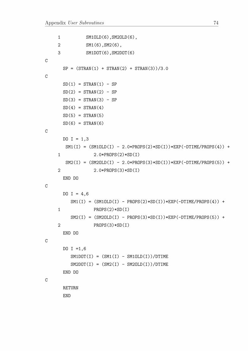
Appendix User Subroutines 74
1 SM1OLD(6),SM2OLD(6),
2 SM1(6),SM2(6),
3 SM1DOT(6),SM2DOT(6)
C
SP = (STRAN(1) + STRAN(2) + STRAN(3))/3.0
C
SD(1) = STRAN(1) - SP
SD(2) = STRAN(2) - SP
SD(3) = STRAN(3) - SP
SD(4) = STRAN(4)
SD(5) = STRAN(5)
SD(6) = STRAN(6)
C
DO I = 1,3
SM1(I) = (SM1OLD(I) - 2.0*PROPS(2)*SD(I))*EXP(-DTIME/PROPS(4)) +
1 2.0*PROPS(2)*SD(I)
SM2(I) = (SM2OLD(I) - 2.0*PROPS(3)*SD(I))*EXP(-DTIME/PROPS(5)) +
2 2.0*PROPS(3)*SD(I)
END DO
C
DO I = 4,6
SM1(I) = (SM1OLD(I) - PROPS(2)*SD(I))*EXP(-DTIME/PROPS(4)) +
1 PROPS(2)*SD(I)
SM2(I) = (SM2OLD(I) - PROPS(3)*SD(I))*EXP(-DTIME/PROPS(5)) +
2 PROPS(3)*SD(I)
END DO
C
DO I =1,6
SM1DOT(I) = (SM1(I) - SM1OLD(I))/DTIME
SM2DOT(I) = (SM2(I) - SM2OLD(I))/DTIME
END DO
C
RETURN
END

Appendix User Subroutines 75
A.2.2 UMAT with Four Maxwell Elements (N = 4)
C ******************************************************************
* *
C * U M A T *
C * *
C * AN ABAQUS USER MATERIAL MODEL FOR 3D VISCOELASTICITY *
C * (BASED ON MAXWELL ELEMENTS IN PARALLEL WITH AN ELASTIC SPRING) *
C * *
C * CE521: SOLID MECHANICS *
C * HWK. ASSIGNMENT #2 *
C * *
C * WRITTEN BY : Prof. R. M. Hackett - University of Mississippi *
C * DATE : SPRING 1999 *
C * REVISED BY : CHRIS L. MULLEN- University of Mississippi *
C * DATE : SPRING 1999 *
C * *
C ******************************************************************
C234567890123456789012345678901234567890123456789012345678901234567890
SUBROUTINE UMAT (STRESS,STATEV,DDSDDE,SSE,SPD,SCD,
1 RPL,DDSDDT,DRPLDE,DRPLDT,
2 STRAN,DSTRAN,TIME,DTIME,TEMP,DTEMP,PREDEF,DPRED,CMNAME,
3 NDI,NSHR,NTENS,NSTATV,PROPS,NPROPS,COORDS,DROT,PNEWDT,
4 CELENT,DFGRDO,DFGRD1,NOEL,NPT,LAYER,KSPT,KSTEP,KINC)
C
INCLUDE ’ABA_PARAM.INC’
C
C
CHARACTER*8 CMNAME
DIMENSION STRESS(NTENS),STATEV(NSTATV),
1 DDSDDE(NTENS,NTENS),DDSDDT(NTENS),DRPLDE(NTENS),
2 STRAN(NTENS),DSTRAN(NTENS),TIME(2),PREDEF(1),DPRED(1),
3 PROPS(NPROPS),COORDS(3),DROT(3,3),DFGRD0(3,3),DFGRD1(3,3)
DIMENSION DSTRES(6),D(3,3)
C
C
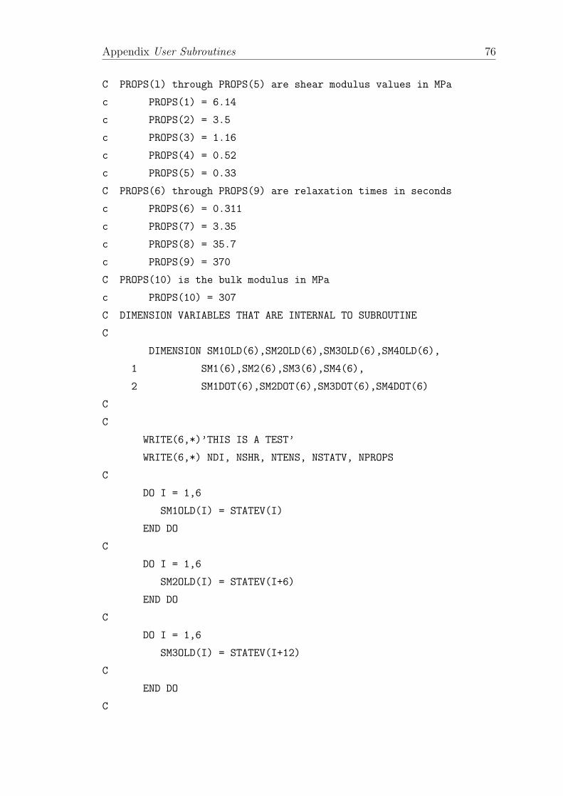
Appendix User Subroutines 76
C PROPS(l) through PROPS(5) are shear modulus values in MPa
c PROPS(1) = 6.14
c PROPS(2) = 3.5
c PROPS(3) = 1.16
c PROPS(4) = 0.52
c PROPS(5) = 0.33
C PROPS(6) through PROPS(9) are relaxation times in seconds
c PROPS(6) = 0.311
c PROPS(7) = 3.35
c PROPS(8) = 35.7
c PROPS(9) = 370
C PROPS(10) is the bulk modulus in MPa
c PROPS(10) = 307
C DIMENSION VARIABLES THAT ARE INTERNAL TO SUBROUTINE
C
DIMENSION SM1OLD(6),SM2OLD(6),SM3OLD(6),SM4OLD(6),
1 SM1(6),SM2(6),SM3(6),SM4(6),
2 SM1DOT(6),SM2DOT(6),SM3DOT(6),SM4DOT(6)
C
C
WRITE(6,*)’THIS IS A TEST’
WRITE(6,*) NDI, NSHR, NTENS, NSTATV, NPROPS
C
DO I = 1,6
SM1OLD(I) = STATEV(I)
END DO
C
DO I = 1,6
SM2OLD(I) = STATEV(I+6)
END DO
C
DO I = 1,6
SM3OLD(I) = STATEV(I+12)
C
END DO
C
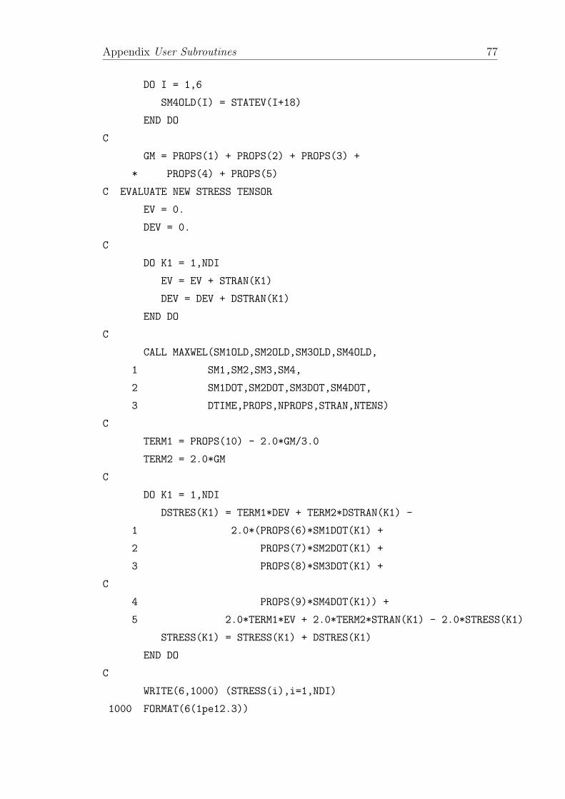
Appendix User Subroutines 77
DO I = 1,6
SM4OLD(I) = STATEV(I+18)
END DO
C
GM = PROPS(1) + PROPS(2) + PROPS(3) +
* PROPS(4) + PROPS(5)
C EVALUATE NEW STRESS TENSOR
EV = 0.
DEV = 0.
C
DO K1 = 1,NDI
EV = EV + STRAN(K1)
DEV = DEV + DSTRAN(K1)
END DO
C
CALL MAXWEL(SM1OLD,SM2OLD,SM3OLD,SM4OLD,
1 SM1,SM2,SM3,SM4,
2 SM1DOT,SM2DOT,SM3DOT,SM4DOT,
3 DTIME,PROPS,NPROPS,STRAN,NTENS)
C
TERM1 = PROPS(10) - 2.0*GM/3.0
TERM2 = 2.0*GM
C
DO K1 = 1,NDI
DSTRES(K1) = TERM1*DEV + TERM2*DSTRAN(K1) -
1 2.0*(PROPS(6)*SM1DOT(K1) +
2 PROPS(7)*SM2DOT(K1) +
3 PROPS(8)*SM3DOT(K1) +
C
4 PROPS(9)*SM4DOT(K1)) +
5 2.0*TERM1*EV + 2.0*TERM2*STRAN(K1) - 2.0*STRESS(K1)
STRESS(K1) = STRESS(K1) + DSTRES(K1)
END DO
C
WRITE(6,1000) (STRESS(i),i=1,NDI)
1000 FORMAT(6(1pe12.3))
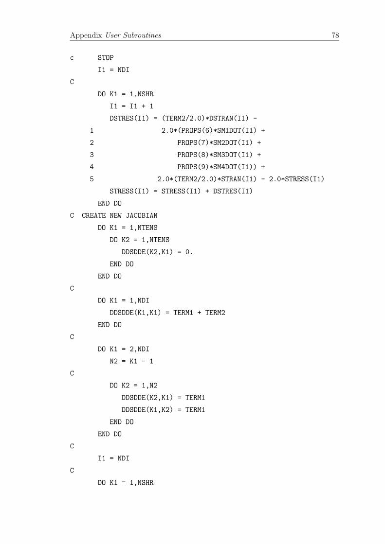
Appendix User Subroutines 78
c STOP
I1 = NDI
C
DO K1 = 1,NSHR
I1 = I1 + 1
DSTRES(I1) = (TERM2/2.0)*DSTRAN(I1) -
1 2.0*(PROPS(6)*SM1DOT(I1) +
2 PROPS(7)*SM2DOT(I1) +
3 PROPS(8)*SM3DOT(I1) +
4 PROPS(9)*SM4DOT(I1)) +
5 2.0*(TERM2/2.0)*STRAN(I1) - 2.0*STRESS(I1)
STRESS(I1) = STRESS(I1) + DSTRES(I1)
END DO
C CREATE NEW JACOBIAN
DO K1 = 1,NTENS
DO K2 = 1,NTENS
DDSDDE(K2,K1) = 0.
END DO
END DO
C
DO K1 = 1,NDI
DDSDDE(K1,K1) = TERM1 + TERM2
END DO
C
DO K1 = 2,NDI
N2 = K1 - 1
C
DO K2 = 1,N2
DDSDDE(K2,K1) = TERM1
DDSDDE(K1,K2) = TERM1
END DO
END DO
C
I1 = NDI
C
DO K1 = 1,NSHR
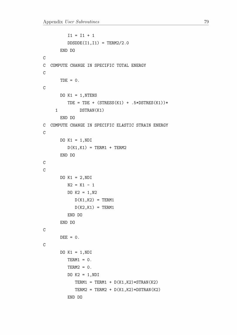
Appendix User Subroutines 79
I1 = I1 + 1
DDSDDE(I1,I1) = TERM2/2.0
END DO
C
C COMPUTE CHANGE IN SPECIFIC TOTAL ENERGY
C
TDE = 0.
C
DO K1 = 1,NTENS
TDE = TDE + (STRESS(K1) + .5*DSTRES(K1))*
1 DSTRAN(K1)
END DO
C COMPUTE CHANGE IN SPECIFIC ELASTIC STRAIN ENERGY
C
DO K1 = 1,NDI
D(K1,K1) = TERM1 + TERM2
END DO
C
C
DO K1 = 2,NDI
N2 = K1 - 1
DO K2 = 1,N2
D(K1,K2) = TERM1
D(K2,K1) = TERM1
END DO
END DO
C
DEE = 0.
C
DO K1 = 1,NDI
TERM1 = 0.
TERM2 = 0.
DO K2 = 1,NDI
TERM1 = TERM1 + D(K1,K2)*STRAN(K2)
TERM2 = TERM2 + D(K1,K2)*DSTRAN(K2)
END DO
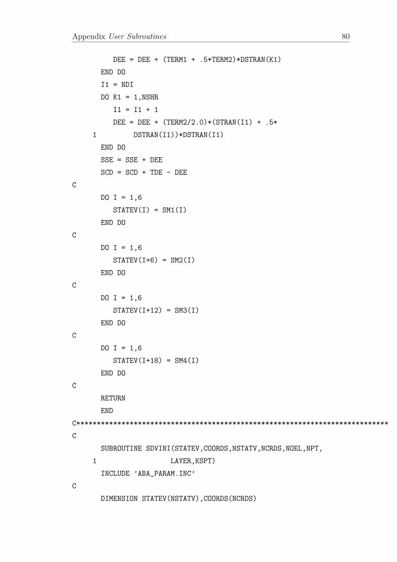
Appendix User Subroutines 80
DEE = DEE + (TERM1 + .5*TERM2)*DSTRAN(K1)
END DO
I1 = NDI
DO K1 = 1,NSHR
I1 = I1 + 1
DEE = DEE + (TERM2/2.0)*(STRAN(I1) + .5*
1 DSTRAN(I1))*DSTRAN(I1)
END DO
SSE = SSE + DEE
SCD = SCD + TDE - DEE
C
DO I = 1,6
STATEV(I) = SM1(I)
END DO
C
DO I = 1,6
STATEV(I+6) = SM2(I)
END DO
C
DO I = 1,6
STATEV(I+12) = SM3(I)
END DO
C
DO I = 1,6
STATEV(I+18) = SM4(I)
END DO
C
RETURN
END
C****************************************************************************
C
SUBROUTINE SDVINI(STATEV,COORDS,NSTATV,NCRDS,NOEL,NPT,
1 LAYER,KSPT)
INCLUDE ’ABA_PARAM.INC’
C
DIMENSION STATEV(NSTATV),COORDS(NCRDS)
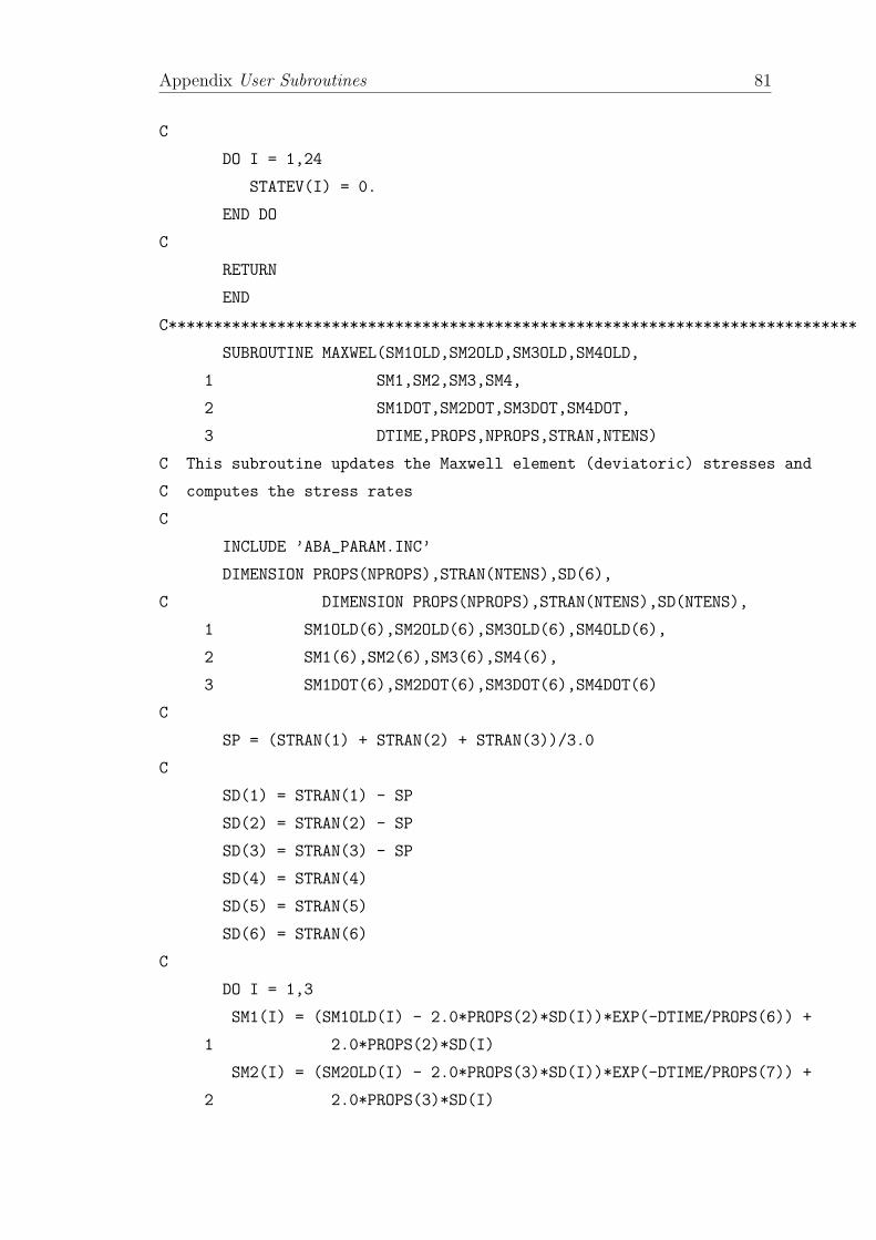
Appendix User Subroutines 81
C
DO I = 1,24
STATEV(I) = 0.
END DO
C
RETURN
END
C****************************************************************************
SUBROUTINE MAXWEL(SM1OLD,SM2OLD,SM3OLD,SM4OLD,
1 SM1,SM2,SM3,SM4,
2 SM1DOT,SM2DOT,SM3DOT,SM4DOT,
3 DTIME,PROPS,NPROPS,STRAN,NTENS)
C This subroutine updates the Maxwell element (deviatoric) stresses and
C computes the stress rates
C
INCLUDE ’ABA_PARAM.INC’
DIMENSION PROPS(NPROPS),STRAN(NTENS),SD(6),
C DIMENSION PROPS(NPROPS),STRAN(NTENS),SD(NTENS),
1 SM1OLD(6),SM2OLD(6),SM3OLD(6),SM4OLD(6),
2 SM1(6),SM2(6),SM3(6),SM4(6),
3 SM1DOT(6),SM2DOT(6),SM3DOT(6),SM4DOT(6)
C
SP = (STRAN(1) + STRAN(2) + STRAN(3))/3.0
C
SD(1) = STRAN(1) - SP
SD(2) = STRAN(2) - SP
SD(3) = STRAN(3) - SP
SD(4) = STRAN(4)
SD(5) = STRAN(5)
SD(6) = STRAN(6)
C
DO I = 1,3
SM1(I) = (SM1OLD(I) - 2.0*PROPS(2)*SD(I))*EXP(-DTIME/PROPS(6)) +
1 2.0*PROPS(2)*SD(I)
SM2(I) = (SM2OLD(I) - 2.0*PROPS(3)*SD(I))*EXP(-DTIME/PROPS(7)) +
2 2.0*PROPS(3)*SD(I)
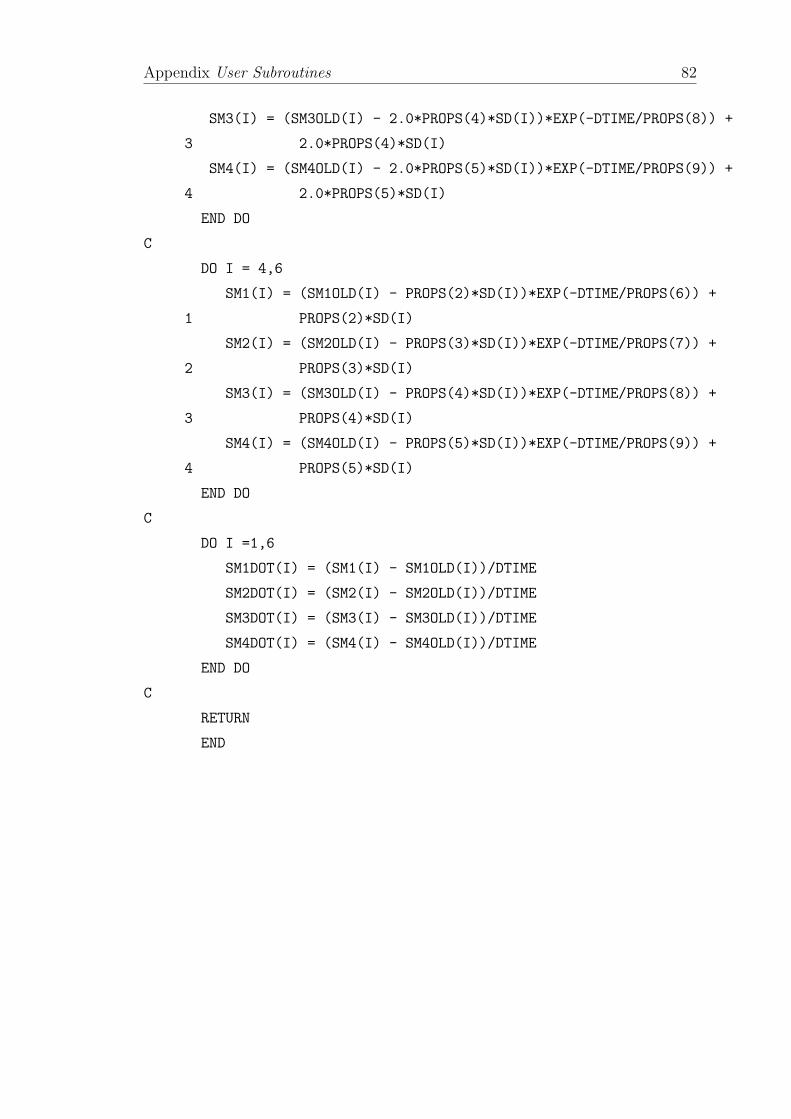
Appendix User Subroutines 82
SM3(I) = (SM3OLD(I) - 2.0*PROPS(4)*SD(I))*EXP(-DTIME/PROPS(8)) +
3 2.0*PROPS(4)*SD(I)
SM4(I) = (SM4OLD(I) - 2.0*PROPS(5)*SD(I))*EXP(-DTIME/PROPS(9)) +
4 2.0*PROPS(5)*SD(I)
END DO
C
DO I = 4,6
SM1(I) = (SM1OLD(I) - PROPS(2)*SD(I))*EXP(-DTIME/PROPS(6)) +
1 PROPS(2)*SD(I)
SM2(I) = (SM2OLD(I) - PROPS(3)*SD(I))*EXP(-DTIME/PROPS(7)) +
2 PROPS(3)*SD(I)
SM3(I) = (SM3OLD(I) - PROPS(4)*SD(I))*EXP(-DTIME/PROPS(8)) +
3 PROPS(4)*SD(I)
SM4(I) = (SM4OLD(I) - PROPS(5)*SD(I))*EXP(-DTIME/PROPS(9)) +
4 PROPS(5)*SD(I)
END DO
C
DO I =1,6
SM1DOT(I) = (SM1(I) - SM1OLD(I))/DTIME
SM2DOT(I) = (SM2(I) - SM2OLD(I))/DTIME
SM3DOT(I) = (SM3(I) - SM3OLD(I))/DTIME
SM4DOT(I) = (SM4(I) - SM4OLD(I))/DTIME
END DO
C
RETURN
END
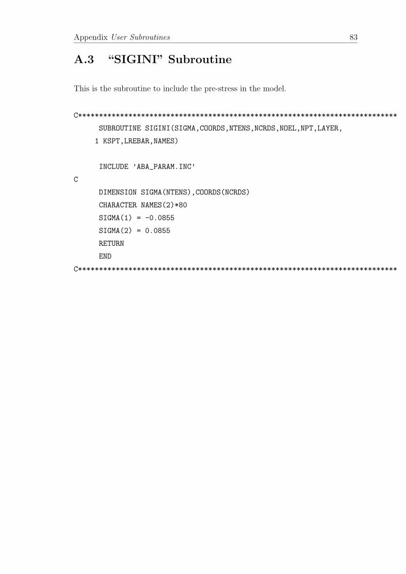
Appendix User Subroutines 83
A.3 “SIGINI” Subroutine
This is the subroutine to include the pre-stress in the model.
C****************************************************************************
SUBROUTINE SIGINI(SIGMA,COORDS,NTENS,NCRDS,NOEL,NPT,LAYER,
1 KSPT,LREBAR,NAMES)
INCLUDE ’ABA_PARAM.INC’
C
DIMENSION SIGMA(NTENS),COORDS(NCRDS)
CHARACTER NAMES(2)*80
SIGMA(1) = -0.0855
SIGMA(2) = 0.0855
RETURN
END
C****************************************************************************
Bibliography
[1] M. Wissler and E. Mazza, “Electromechanical coupling in dielectric elastomer
actuators,” Sensors and Actuators A: Physical, vol. 138, no. 2, pp. 384–393,
2007.
[2] X. Zhao and Z. Suo, “Method to analyze programmable deformation of di-
electric elastomer layers,” Applied Physics Letters, vol. 93, no. 25, p. 251902,
2008.
[3] A. Vinogradov, J. Su, C. Jenkins, and Y. Bar-Cohen, “State-of-the-art devel-
opments in the field of electroactive polymers,” in Material Research Society
Symposium Proceedings, vol. 889, pp. 51–56, 2006.
[4] G. Kofod and P. Sommer-Larsen, “Some aspects of large strain actuation in
dielectric elastomers,” in 12th International Symposium on Electrets, pp. 208–
211, 2005.
[5] Y. Bar-Cohen, “Electro-active polymers: current capabilities and challenges,”
in Proceedings of the SPIE Smart Structures and Materials Symposium, EA-
PAD Conference, SanDiego, CA, vol. 4695, pp. 1–7, March 2002.
[6] N. Goulbourne, E. Mockensturm, and M. Frecker, “A nonlinear model for
dielectric elastomer membranes,” Journal of Applied Mechanics, vol. 72,
pp. 899–906, 2005.
[7] M. T. Wissler, Modeling Dielectric Elastomer Actuators. PhD thesis, Swiss
Federal Institute Of Technology, Zurich, 2007.
[8] A. Wineman, “Nonlinear viscoelastic solids–a review,” Mathematics and Me-
chanics of Solids, vol. 14, no. 3, pp. 300–366, 2009.
84
Bibliography 85
[9] A. V. Tobolsky and R. D. Andrews, “Systems manifesting superposed elastic
and viscous behavior,” The Journal of Chemical Physics, vol. 13, no. 1, pp. 3–
27, 1945.
[10] Y. M. Haddad, Viscoelasticity of engineering materials, p. xix. Chapman &
Hall, 1995.
[11] H. Zhang and L. Li, “Modeling inclusion problems in viscoelastic materials
with the extended finite element method,” Finite Elements in Analysis and
Design, vol. 45, no. 10, pp. 721–729, 2009.
[12] Wikipedia, “Viscoelasticity.” http://en.wikipedia.org/wiki/Viscoelasticity,
October 2009.
[13] L. Boltzmann, “Zur theorie der elastischen nachwirkung,” In:(Sec. Ed. ed.),
Mathematisch - Naturwissenschaftliche Classe, vol. 70, pp. 275–306, 1874.
[14] M. Kaliske and H. Rothert, “Formulation and implementation of three-
dimensional viscoelasticity at small and finite strains,” Computational Me-
chanics, vol. 19, no. 3, pp. 228–239, 1997.
[15] A. Kaye College of Aeronautics, no. 134, 1962.
[16] B. Bernstein, E. A. Kearsley, and L. J. Zapas, “A study of stress relaxation
with finite strain,” Transactions of the Society of Rheology, no. 7, pp. 391–410,
1963.
[17] W. T. Read, Jr., “Stress analysis for compressible viscoelastic materials,”
Journal of Applied Physics, vol. 21, pp. 671–674, 1950.
[18] E. H. Lee, “Stress analysis in viscoelastic materials,” Journal of Applied
Physics, vol. 27, no. 7, pp. 665–672, 1956.
[19] E. H. Lee, “Stress analysis for linear viscoelastic materials,” Rheologica Acta,
vol. 1, pp. 426–430, 1961.
[20] B. D. Coleman and W. Noll, “Foundations of linear viscoelasticity,” Review
of Modern Physics, vol. 33, no. 2, pp. 239–249, 1961.
[21] A. C. Pipkin, “Small finite deformations of viscoelastic solids,” Review of
Modern Physics, 1964.
Bibliography 86
[22] A. Green and R. S. Rivlin, “The mechanics of non-linear materials with mem-
ory part i,” Archive for Rational Mechanics and Analysis, vol. 1, no. 1, pp. 1
– 21, 1957.
[23] W. Noll, “A mathematical theory of the mechanical behavior of continuous
media,” Archive for Rational Mechanics and Analysis, vol. 2, no. 1, pp. 197–
226, 1958.
[24] O. Zienkiewicz, M. Watson, and I. King, “A numerical method of visco-elastic
stress analysis,” International Journal of Mechanical Sciences, 1968.
[25] R. L. Taylor, K. S. Pister, and G. L. Goudreau, “Thermomechanical anal-
ysis of viscoelastic solids,” International Journal for Numerical Methods in
Engineering, vol. 2, no. 1, pp. 45–59, 1970.
[26] A. C. Pipkin and T. G. Rogers, “A non-linear integral representation for vis-
coelastic behaviour,” Journal of the Mechanics and Physics of Solids, vol. 16,
no. 1, pp. 59–72, 1968.
[27] R. A. Schapery, “On the characterization of nonlinear viscoelastic materials,”
Polymer Engineering & Science, vol. 9, no. 4, pp. 295–310, 1969.
[28] Y. Partom and I. Schanin, “Modeling nonlinear viscoelastic response,” Poly-
mer Engineering & Science, vol. 23, no. 15, pp. 849–859, 1983.
[29] B. Keren, Y. Partom, and Z. Rosenberg, “Nonlinear viscoelastic response
in two dimensions - numerical modeling,” Polymer Engineering & Science,
vol. 24, no. 18, pp. 1409–1416, 1984.
[30] R. W. Rendell, K. L. Ngai, G. R. Fong, A. F. Yee, and R. J. Bankert, “Non-
linear viscoelasticity and yield: Application of a coupling model,” Polymer
Engineering & Science, vol. 27, no. 1, pp. 2–15, 1987.
[31] K. C. Gramoll, D. A. Dillard, and H. F. Brinson, “A stable numerical solution
method for in-plane loading of nonlinear viscoelastic laminated orthotropic
materials,” Composite Structures, vol. 13, no. 4, pp. 251–274, 1989.
[32] P. Krishnaswamy, M. E. Tuttle, A. F. Emery, and J. Ahmad, “Finite ele-
ment modelling of crack tip behaviour in viscoelastic materials. part i: Lin-
ear behaviour,” International Journal for Numerical Methods in Engineering,
vol. 30, no. 2, pp. 371–387, 1990.
Bibliography 87
[33] G. U. Losi and W. G. Knauss, “Thermal stresses in nonlinearly viscoelastic
solids,” Journal of Applied Mechanics, vol. 59, no. 25, pp. S43–S49, 1992.
[34] G. Ghazlan, S. Caperaa, and C. Petit, “An incremental formulation for the
linear analysis of thin viscoelastic structures using generalized variables,” In-
ternational Journal for Numerical Methods in Engineering, vol. 38, no. 19,
pp. 3315–3333, 1995.
[35] S. P. Zaoutsos, G. C. Papanicolaou, and A. H. Cardon, “On the non-linear
viscoelastic behaviour of polymer-matrix composites,” Composites Science
and Technology, vol. 58, no. 6, pp. 0266–3538, 1998.
[36] S. Reese and S. Govindjee, “Theoretical and numerical aspects in the thermo-
viscoelastic material behaviour of rubber-like polymers,” Mechanics of Time-
Dependent Materials, vol. 1, no. 4, pp. 357–396, 1997.
[37] J. R. Masuero and G. J. Creus, “Finite elements analysis of viscoelastic frac-
ture,” International Journal of Fracture, vol. 60, no. 3, pp. 267–282, 1993.
[38] C. S. Drapaca, S. Sivaloganathan, and G. Tenti, “Nonlinear constitutive
laws in viscoelasticity,” Mathematics and Mechanics of Solids, vol. 12, no. 5,
pp. 475–501, 2007.
[39] R. S. Lakes, Viscoelastic Solids, ch. 6. CRC Press, October 1998.
[40] Wikipedia, “Viscoelasticity.” http://en.wikipedia.org/wiki/Creep_(deformation),
October 2009.
[41] D. V. Rosato, D. V. Rosato, and M. Rosato, Plastics Design Handbook.
Springer - Verlag, 2001.
[42] Instron, “Creep and stress-relaxation test.”
http://www.instron.us/wa/applications/test_types/creep_stress_relax.aspx,
April 2010.
[43] Y. Bar-Cohen, ed., Electroactive Polymer (EAP) Actuators as Artificial Mus-
cles: Reality, Potential, and Challenges. SPIE Publications, second ed., 2004.
[44] J. C. Koo, K.-M. Jung, M.-Y. Jung, H. Choi, J. Nam, and Y. Lee, “Effect
of pre-strain on the antagonistically driven dielectric polymer actuator,” Key
Engineering Materials, vol. 306/308; Part 2, pp. 1187–1192, 2006.
Bibliography 88
[45] J. W. Fox, “Electromechanical characterization of the static and dynamic
response of dielectric elastomer membranes,” Master’s thesis, Virginia Poly-
technic Institute and State University, Blacksburg, Virginia, 2007.
[46] E. Biddiss and T. Chaua, “Dielectric elastomers as actuators for upper limb
prosthetics: Challenges and opportunities,” Medical Engineering & Physics,
vol. 30, no. 4, pp. 403–418, 2008.
[47] R. Shankar, T. K. Ghosh, and R. J. Spontak, “Dielectric elastomers as next-
generation polymeric actuators,” Soft Matter, vol. 3, pp. 1116–1129, 2007.
[48] M. Wissler and E. Mazza, “Modeling and simulation of dielectric elastomer
actuators,” Smart Mater. Struct., vol. 14, no. 6, pp. 1396–1402, 2005.
[49] J. Fox and N. Goulbourne, “On the dynamic electromechanical loading of
dielectric elastomer membranes,” Journal of the Mechanics and Physics of
Solids, vol. 56, no. 8, pp. 2669–2686, 2008.
[50] H. Wang, J. Zhu, and K. Ye, “Simulation, experimental evaluation and per-
formance improvement of a cone dielectric elastomer actuator,” Journal of
Zhejiang University SCIENCE A, vol. 10, no. 9, pp. 1296–1304, 2009.
[51] P. Lochmatter, G. Kovacs, and S. Michel, “Characterization of dielectric elas-
tomer actuators based on a hyperelastic film model,” Sensors and Actuators
A: Physical, vol. 135, no. 2, pp. 748–757, 2007.
[52] O. Yeoh, “Characterization of elastic properties of carbon-black-filled rubber
vulcanizates,” Rubber Chem. Technol., vol. 63, pp. 792–805, 1990.
[53] H. R. Choi, K. Jung, S. Ryew, J.-D. Nam, J. Jeon, J. C. Koo, and
K. Tanie, “Biomimetic soft actuator: Design, modeling, control, and appli-
cations,” IEEE/ASME TRANSACTIONS ON MECHATRONICS, vol. 10,
no. 5, pp. 581–593, 2005.
[54] M. R. Begley, H. Bart-Smith, O. N. Scott, M. H. Jones, and M. L. Reed, “The
electro-mechanical response of elastomer membranes coated with ultra-thin
metal electrodes,” Journal of the Mechanics and Physics of Solids, 2005.
[55] M. R. Begley and T. J. Mackin, “Spherical indentation of freestanding circular
thin films in the membrane regime,” Journal of the Mechanics and Physics
of Solids, vol. 52, no. 9, pp. 2005 – 2023, 2004.
Bibliography 89
[56] F. Carpi and D. D. Rossi, “Biomimetic dielectric elastomer actuators,” in
Biomedical Robotics and Biomechatronics, 2006. BioRob 2006. The First
IEEE/RAS-EMBS International Conference on, pp. 1073–1078, 2006.
[57] E. M. Mockensturm and N. Goulbourne, “Dynamic response of dielectric
elastomers,” International Journal of Non-Linear Mechanics, vol. 41, no. 3,
pp. 388–395, 2006.
[58] J.-S. Plante and S. Dubowsky, “On the properties of dielectric elastomer
actuators and their design implications,” Smart Materials and Structures,
vol. 16, no. 2, pp. 227–236, 2007.
[59] R. E. Pelrine, R. D. Kornbluh, and J. P. Joseph, “Electrostriction of poly-
mer dielectrics with compliant electrodes as a means of actuation,” Sensors
and Actuators A: Physical, vol. 64, no. 1, pp. 77 – 85, 1998. Tenth IEEE
International Workshop on Micro Electro Mechanical Systems.
[60] J.-S. Plante and S. Dubowsky, “On the performance mechanisms of dielectric
elastomer actuators,” Sensors and Actuators A: Physical, vol. 137, no. 1,
pp. 96–109, 2007.
[61] J. Fox and N. Goulbourne, “Electric field-induced surface transformations
and experimental dynamic characteristics of dielectric elastomer membranes,”
Journal of the Mechanics and Physics of Solids, vol. 57, no. 8, pp. 1417–1435,
2009.
[62] A. Green and J. Adkins, Large Elastic Deformations. Oxford University Press,
London, 1970.
[63] R. Shankar, T. K. Ghosh, and R. J. Spontak, “Mechanical and actuation
behavior of electroactive nanostructured polymers,” Sensors and Actuators
A: Physical, vol. 151, no. 1, pp. 46–52, 2009.
[64] F. Carpi, D. D. Rossi, R. Kornbluh, R. Pelrine, and P. Sommer-Larsen, eds.,
Dielectric Elastomers as Electromechanical Transducers, ch. V. Fundamen-
tals, Materials, Devices, Models and Applications of an Emerging Electroac-
tive Polymer Technology, Elsevier Ltd., 2008.
[65] O. Zienkiewicz and R. Taylor, The Finite Element Method for Solid and Struc-
tural Mechanics. Elsevier Butterworth-Heinemann, sixth ed., 2005.
Bibliography 90
[66] J. Bonet and R. D. Wood, Nonlinear Continuum Mechanics for Finite Ele-
ment Analysis. Cambridge University Press, 1997.
[67] G. Mase, Schaum’s Outline of Continuum Mechanics. McGraw-Hill, 1969.
[68] G. A. Holzapfel, Nonlinear Solid Mechanics: A Continuum Approach for En-
gineering. Wiley, first ed., 2000.
[69] J. Simo and T. Hughes, Computational Inelasticity. Springer, 1998.
[70] T. Belytschko, W. K. Liu, and B. Moran, Nonlinear Finite Elements for
Continua and Structures. Wiley, first ed., 2000.
[71] Dassault Systemes Simulia Corp., Providence, RI, USA, Abaqus User Subrou-
tines Reference Manual, 2009.
[72] Dassault Systemes Simulia Corp., Providence, RI, USA, Abaqus Analysis
User’s Manual, 2009.
[73] Dassault Systemes Simulia Corp., Providence, RI, USA, Abaqus Verification
Manual, 2009.
[74] R. M. Hackett, “An abaqus user material model for 3d viscoelasticity.”
http://www.olemiss.edu/courses/ce521/f77.html, 1999. University of
Mississippi.