
Institut de genie nucl´ eaire´ Ecole Polytechnique de ...
31
The neutron diffusion equation Alain H ´ ebert [email protected] Institut de g ´ enie nucl ´ eaire ´ Ecole Polytechnique de Montr ´ eal ENE6103: Week 2 The neutron diffusion equation – 1/31
Transcript of Institut de genie nucl´ eaire´ Ecole Polytechnique de ...
The neutron diffusion equationAlain Hebert
Institut de genie nucleaire
Ecole Polytechnique de Montreal
ENE6103: Week 2 The neutron diffusion equation – 1/31

Content (week 2) 1
Full core calculationsThe steady-state diffusion equationContinuity and boundary conditions
The finite homogeneous reactorCartesian coordinate systemSpherical coordinate systemCylindrical coordinate system
The heterogeneous 1D slab reactorTwo region example
ENE6103: Week 2 The neutron diffusion equation – 2/31

Full core calculations 1
The full-core calculation consists of solving a simplified transport equation, either thediffusion equation or the simplified Pn equation.
This solution can be performed either in transient or steady-state conditions, using asmall number of energy groups (generally, G = 2 is sufficient).
A steady-state full-core calculation generally uses the effective multiplication factorKeff as eigenvalue. Another possible choice of eigenvalue is to select a poisonconcentration or the position of a reactivity device.
Full-core calculations offer the possibility of accurately representing the reactorboundary. A correct representation of neutron leakage will be possible, as neutronseffectively escape the reactor domain through its boundary.
ENE6103: Week 2 The neutron diffusion equation – 3/31
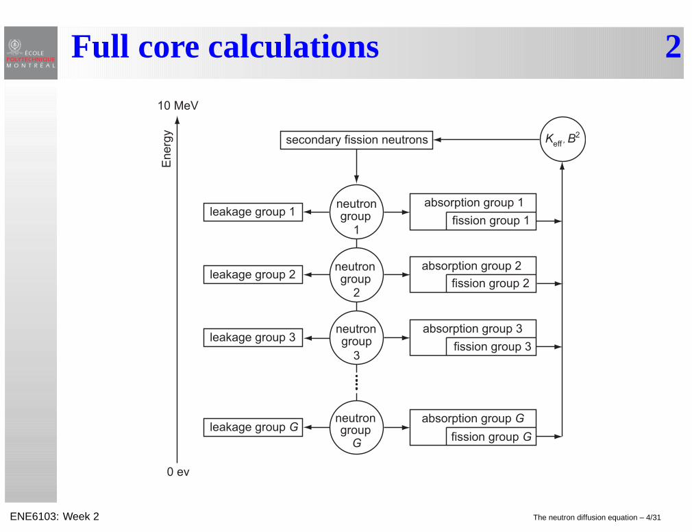
Full core calculations 2
neutrongroup
1
neutrongroup
2
neutrongroup
3
neutrongroup
G
leakage group 1
leakage group 2
leakage group 3
leakage group G
secondary fission neutrons
absorption group 1
absorption group 2
absorption group 3
absorption group G
fission group 1
fission group 2
fission group 3
fission group G
Keff
, B2
10 MeV
0 ev
En
erg
y
ENE6103: Week 2 The neutron diffusion equation – 4/31

Full core calculations 3
We will first investigate the steady-state solution of the transport equation over the completereactor domain. The neutron balance over any control domain in energy group g is written
Leakage rate + Collision rate = Sources
or, in symbolic form,
∇ · Jg(r) + Σg(r)φg(r) = Qg(r)(1)
where Jg(r) is the neutronic current. The scalar product of the neutronic current with N isequal to the net number of neutrons crossing the arbitrary surface per unit surface and time.
ENE6103: Week 2 The neutron diffusion equation – 5/31
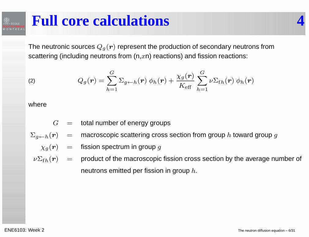
Full core calculations 4
The neutronic sources Qg(r) represent the production of secondary neutrons fromscattering (including neutrons from (n,xn) reactions) and fission reactions:
Qg(r) =GX
h=1
Σg←h(r) φh(r) +χg(r)
Keff
GX
h=1
νΣfh(r) φh(r)(2)
where
G = total number of energy groups
Σg←h(r) = macroscopic scattering cross section from group h toward group g
χg(r) = fission spectrum in group g
νΣfh(r) = product of the macroscopic fission cross section by the average number of
neutrons emitted per fission in group h.
ENE6103: Week 2 The neutron diffusion equation – 6/31
Full core calculations 5
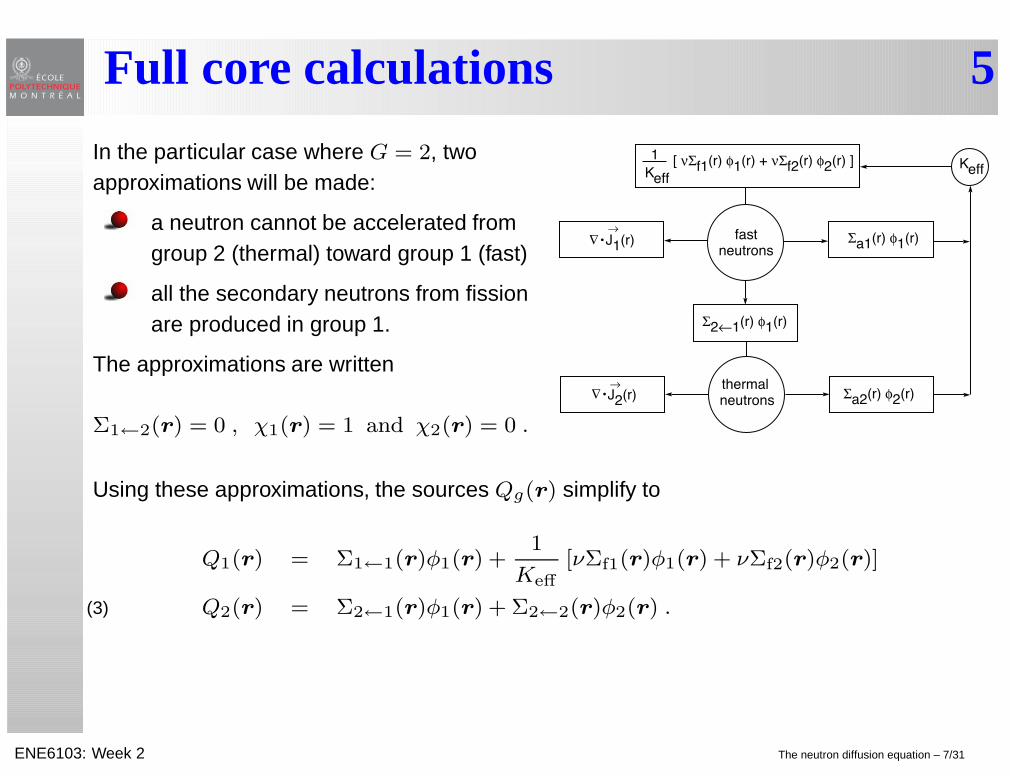
In the particular case where G = 2, twoapproximations will be made:
a neutron cannot be accelerated fromgroup 2 (thermal) toward group 1 (fast)
all the secondary neutrons from fissionare produced in group 1.
The approximations are written
Σ1←2(r) = 0 , χ1(r) = 1 and χ2(r) = 0 .
1
Keff
[ νΣf1(r) φ1(r) + νΣf2(r) φ2(r) ]
Σ2←1(r) φ1(r)
Σa1(r) φ1(r)
Σa2(r) φ2(r)
Keff
J1(r)
J2(r)
→
→
∆
•
∆ •
fast
thermal
neutrons
neutrons
Using these approximations, the sources Qg(r) simplify to
Q1(r) = Σ1←1(r)φ1(r) +1
Keff
[νΣf1(r)φ1(r) + νΣf2(r)φ2(r)]
Q2(r) = Σ2←1(r)φ1(r) + Σ2←2(r)φ2(r) .(3)
ENE6103: Week 2 The neutron diffusion equation – 7/31

Full core calculations 6
We have obtained a balance equation for a steady-state reactor, corresponding to thesituation where the leakage and absorption rates are exactly equal to the productionrate of new neutrons, at all times, in each energy group.
In this case, the effective multiplication factor Keff is an artifact (or an eigenvalue) thatsatisfies this equality. This factor is expected to be close to one for a reactor in anominal situation.
Later, we will show how an additional term can be added to the transport equation torepresent transient behavior of the reactor in cases where the equality is not met.
Equation (1) must be solved on the scale of the complete reactor, correctly taking intoaccount the position of its boundaries.
Solution of Eq. (1) requires additional information to relate the neutron flux and current.Two approaches are possible to obtain this information:
use a spherical harmonics (Pn) or discrete ordinate (SN ) approach. A legacyalternative is to use a variant of the Pn method based on the simplified Pn
equation.
relate the neutron current to the gradient of the neutron flux using the Fick law.This second choice will lead to the diffusion equation.
ENE6103: Week 2 The neutron diffusion equation – 8/31

The steady-state diffusion equation 1
The Fick law is a heuristic relation between the neutron current and the gradient of theneutron flux, translating the fact that neutrons have a tendency to migrate from regionswhere they are more numerous to regions where they are less. This relation is known to beacceptable on the scale of the complete reactor, but not at the level of lattice calculationswhere it breaks down. It is written
Jg(r) = − Dg (r)∇φg(r)(4)
where Dg(r) is a 3 × 3 diagonal tensor containing directional diffusion coefficients.
Non-directional diffusion coefficients are generally sufficient to represent streaming effects inthe lattice. In this case, the three diagonal components are simply set to the same value.Directional diffusion coefficients are more closely related to the B1 heterogeneous streamingeffect occurring when long streaming channels or planes are open in the reactor. The unit ofthe diffusion coefficient is the centimeter (cm).
Substituting Eq. (4) into Eq. (1), we get the neutron diffusion equation as
− ∇ · Dg(r)∇φg(r) + Σg(r)φg(r) = Qg(r) .(5)
ENE6103: Week 2 The neutron diffusion equation – 9/31

The steady-state diffusion equation 2The next step consists in subtracting the within-group scattering rate from both sides ofEq. (5). We obtain the one-speed neutron diffusion equation as
− ∇ · Dg(r)∇φg(r) + Σrg(r)φg(r) = Q⋄g(r)(6)
where Σrg(r) = Σg(r) − Σg←g(r) is the removal cross section and where Q⋄g(r) is written
Q⋄g(r) =GX
h=1
h6=g
Σg←h(r)φh(r) +χg(r)
Keff
GX
h=1
νΣfh(r)φh(r) .(7)
In the two–energy group case (G = 2), Eq. (7) simplifies to
Q⋄1(r) =1
Keff
[νΣf1(r)φ1(r) + νΣf2(r)φ2(r)]
Q⋄2(r) = Σ2←1(r)φ1(r) .(8)
The neutron diffusion equation can be solved analytically in academic cases or usingstandard numerical analysis techniques such as the finite difference or finite elementmethod.
ENE6103: Week 2 The neutron diffusion equation – 10/31

The steady-state diffusion equation 3Substituting the source term from Eq. (7) into Eq. (6), we get the multigroup form of thesteady-state neutron diffusion equation:
− ∇ · Dg(r)∇φg(r) + Σrg(r)φg(r)
=
GX
h=1
h6=g
Σg←h(r)φh(r) +χg(r)
λ
GX
h=1
νΣfh(r)φh(r) .(9)
Equation (9) is an eigenproblem, whose solution behaves in a typical way:
A trivial solution of Eq. (9) is φg(r) = 0 , ∀r. Many non-trivial solutions of Eq. (9) existfor different eigenvalues λ. The largest eigenvalue in absolute value corresponds tothe fundamental solution of the eigenproblem and is equal to the effectivemultiplication factor Keff of the reactor. Only the fundamental solution has a physicalmeaning. The eigenspectrum of Eq. (9) is the set of all its eigenvalues (includingKeff ).
Only the fundamental solution can lead to a positive neutron flux φg(r) over thereactor domain. The other solutions are called neutron flux harmonics and lead tooscillating values of the flux, sometime positive, sometime negative.
ENE6103: Week 2 The neutron diffusion equation – 11/31

The steady-state diffusion equation 4Every solution of Eq. (9) can be renormalized with an arbitrary normalization constant.If φg(r) is a solution, then C φg(r) is also a solution for any value of constant C. Thenormalization constant is generally computed from the knowledge of the reactor power:
GX
g=1
Z
Vd3r Hg(r)φg(r) = P(10)
where V is the volume of the reactor, Hg(r) is the H–factor and P is the power of thereactor. The H–factor permits the computation of the recoverable energy produced bythe reactor.
ENE6103: Week 2 The neutron diffusion equation – 12/31

The steady-state diffusion equation 5It is possible to find a mathematical adjoint to Eq. (9). This adjoint equation has thesame eigenspectrum as Eq. (9).
The mathematical adjoint of Eq. (9) is obtained by permuting primary and secondary groupindices. It is written
− ∇ · Dg(r)∇φ∗g(r) + Σrg(r)φ∗g(r)
=GX
h=1
h6=g
Σh←g(r)φ∗h(r) +νΣfg(r)
λ
GX
h=1
χh(r)φ∗h(r)(11)
where φ∗g(r) is the adjoint flux or adjoint flux harmonics. The particular case with G = 1 issaid to be self-adjoint as it corresponds to the case where φ∗g(r) = φg(r). The adjoint fluxcan also be renormalized with an arbitrary normalization constant. It is generally normalizedusing the following arbitrary relation:
GX
g=1
Z
Vd3r χfg(r)φ∗g(r) = 1 .(12)
ENE6103: Week 2 The neutron diffusion equation – 13/31
Continuity and boundary conditions 1The neutron flux is a continuous distribution of r and the neutron current must be continuousacross an infinite plane placed at abscissa x0. The flux continuity condition at this point is
φg(x−0, y, z) = φg(x+
0, y, z) ∀ y and z .(13)
The neutron current continuity condition is written after introducing the unit normalN = (1, 0, 0), perpendicular to the infinite plane. We write
Jg(x−0, y, z) · N = Jg(x+
0, y, z) · N ∀ y and z .(14)
Using the Fick law from Eq. (4), we obtain
− Dg(x−0, y, z)∇φg(x−
0, y, z) · N = − Dg (x+
0, y, z)∇φg(x+
0, y, z) · N ∀ y and z(15)
or
Dg (x−0 , y, z)d
dxφg(x, y, z)
˛
˛
˛
x=x−0
= Dg(x+0 , y, z)
d
dxφg(x, y, z)
˛
˛
˛
x=x+
0
∀ y et z .(16)
Equation (16) indicates that the neutron flux gradient is discontinuous at each point of thedomain where the diffusion coefficient is discontinuous.
ENE6103: Week 2 The neutron diffusion equation – 14/31
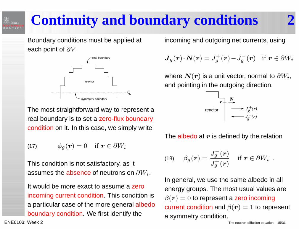
Continuity and boundary conditions 2Boundary conditions must be applied ateach point of ∂V .
C L
reactor
real boundary
symmetry boundary
The most straightforward way to represent areal boundary is to set a zero-flux boundarycondition on it. In this case, we simply write
φg(r) = 0 if r ∈ ∂Wi(17)
This condition is not satisfactory, as itassumes the absence of neutrons on ∂Wi.
It would be more exact to assume a zeroincoming current condition. This condition isa particular case of the more general albedoboundary condition. We first identify the
incoming and outgoing net currents, using
Jg(r) ·N(r) = J+g (r)−J−g (r) if r ∈ ∂Wi
where N(r) is a unit vector, normal to ∂Wi,and pointing in the outgoing direction.
reactor
Nr
J +(r)
J −(r)
g
g
The albedo at r is defined by the relation
βg(r) =J−g (r)
J+g (r)
if r ∈ ∂Wi .(18)
In general, we use the same albedo in allenergy groups. The most usual values areβ(r) = 0 to represent a zero incomingcurrent condition and β(r) = 1 to representa symmetry condition.
ENE6103: Week 2 The neutron diffusion equation – 15/31
Continuity and boundary conditions 3The incoming and outgoing net currents can be obtained from the neutron current and fluxdistributions provided the angular flux is represented by a limited P1 expansion
J−g (r) =1
4φg(r) −
1
2Jg(r) · N(r) and J+
g (r) =1
4φg(r) +
1
2Jg(r) · N(r) .(19)
Substituting Eqs. (19) into (18) and using the Fick law (4), we obtain the albedo boundarycondition as
Dg (r)∇φg(r) · N(r) +1
2
1 − β(r)
1 + β(r)φg(r) = 0 if r ∈ ∂Wi(20)
where ∂Wi is the fraction of ∂V where the albedo boundary condition is applied.
The Fick law and the P1 approximation introduce an error in the zero incoming currentcondition that can be reduced by using a value of β(r) slightly above zero. We recommendto represent the zero incoming current condition using the value β(r) = 0.031758.
Another particular case is the symmetry condition obtained by setting the albedo to valueβ(r) = 1. In this case, Eq. (20) reduces to
∇φg(r) · N(r) = 0 if r ∈ ∂Wi .(21)
ENE6103: Week 2 The neutron diffusion equation – 16/31
The finite homogeneous reactor 1Consider an homogeneous and finite reactor surrounded by zero-flux or symmetryboundary conditions. The nuclear properties of the reactor are independent of space
We use non-directional diffusion coefficients.
Equation (9) simplifies to
−Dg∇2φg(r) + Σrg φg(r) =
GX
h=1
h6=g
Σg←h φh(r) +χg
Keff
GX
h=1
νΣfh φh(r) .(22)
It is possible to factorize the flux according to
φg(r) = ψ(r)ϕg .(23)
Substituting Eq. (23) into Eq. (22), we obtain
−∇2ψ(r)
ψ(r)= −
Σrg
Dg+
1
Dgϕg
8
>
>
<
>
>
:
GX
h=1
h6=g
Σg←h ϕh +χg
Keff
GX
h=1
νΣfh ϕh
9
>
>
=
>
>
;
.(24)
ENE6103: Week 2 The neutron diffusion equation – 17/31

The finite homogeneous reactor 2We note that the left side of Eq. (24) is independent of the neutron energy whereas its rightside is independent of the position in reactor. This fact is only possible if each side ofEq. (24) is itself equal to the same constant. This constant was set equal to B2, the bucklingof the reactor. We therefore obtain two independent equations as
∇2ψ(r) +B2ψ(r) = 0(25)
andˆ
Dg B2 + Σrg
˜
ϕg =GX
h=1
h6=g
Σg←h ϕh +χg
Keff
GX
h=1
νΣfh ϕh .(26)
Equation (25) is a Laplace equation, an eigenproblem whose eigenvalue is the buckling B2.Its solution is a function of the shape and size of the reactor and of the boundary conditions:
Zero-flux boundary condition: ψ(r) = 0 if r ∈ ∂Wi
Symmetry boundary condition: ∇ψ(r) · N(r) = 0 if r ∈ ∂Wi.
Equation (25) has many non-trivial solutions, each of them corresponding to an element ofits eigenspectrum, but only the fundamental solution corresponds to a positive neutron fluxeverywhere in the domain.
ENE6103: Week 2 The neutron diffusion equation – 18/31

Cartesian coordinate system 1The Cartesian coordinate system is the most usual choice for real application problems. Inthis case, the Laplace operator is written
∇2ψ =∂2ψ
∂x2+∂2ψ
∂y2+∂2ψ
∂z2.(27)
Let us consider a prismatic homogeneous reactor of dimension Lx × Ly × Lz. In this case,the fundamental solution of Eq. (25) is
ψ(x, y, z) = C sinπx
Lxsin
πy
Lysin
πz
Lz.(28)
The Cartesian domain is defined over 0 ≤ x ≤ Lx, 0 ≤ y ≤ Ly and 0 < z < Lz . A zero-fluxboundary condition is imposed on the surface of the domain. The normalization constant Cis arbitrary as both Eqs. (25) and (26) are eigenproblems.
The corresponding critical buckling is
B2 =
„
π
Lx
«2
+
„
π
Ly
«2
+
„
π
Lz
«2
.(29)
ENE6103: Week 2 The neutron diffusion equation – 19/31

Spherical coordinate system 1The Laplace operator is written
∇2ψ =1
r2 sinθ
»
sinθ∂
∂r
„
r2∂ψ
∂r
«
+∂
∂θ
„
sinθ∂ψ
∂θ
«
+1
sinθ
∂2ψ
∂ǫ2
–
.(30)
θ
ε
r
X
Y
Z
r
The fundamental solution of Eq. (25)represents the neutron flux in a sphericalreactor of radius R. A zero-flux boundarycondition is imposed at r = R (i.e.,ψ(R) = 0). The fundamental solution iswritten
ψ(r) =C
rsin
πr
R(31)
with the critical buckling equal to
B2 =“ π
R
”2
.(32)
ENE6103: Week 2 The neutron diffusion equation – 20/31
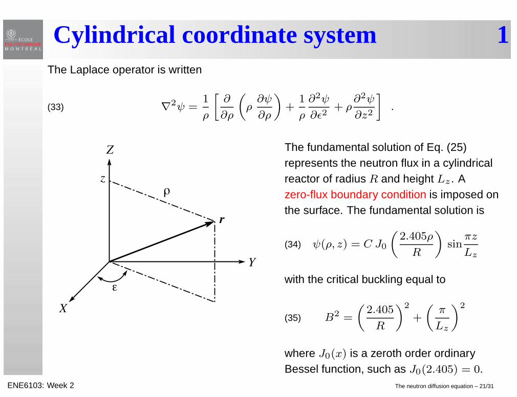
Cylindrical coordinate system 1The Laplace operator is written
∇2ψ =1
ρ
»
∂
∂ρ
„
ρ∂ψ
∂ρ
«
+1
ρ
∂2ψ
∂ǫ2+ ρ
∂2ψ
∂z2
–
.(33)
ε
r
X
Y
Z
ρ z
The fundamental solution of Eq. (25)represents the neutron flux in a cylindricalreactor of radius R and height Lz. Azero-flux boundary condition is imposed onthe surface. The fundamental solution is
ψ(ρ, z) = C J0
„
2.405ρ
R
«
sinπz
Lz(34)
with the critical buckling equal to
B2 =
„
2.405
R
«2
+
„
π
Lz
«2
(35)
where J0(x) is a zeroth order ordinaryBessel function, such as J0(2.405) = 0.
ENE6103: Week 2 The neutron diffusion equation – 21/31
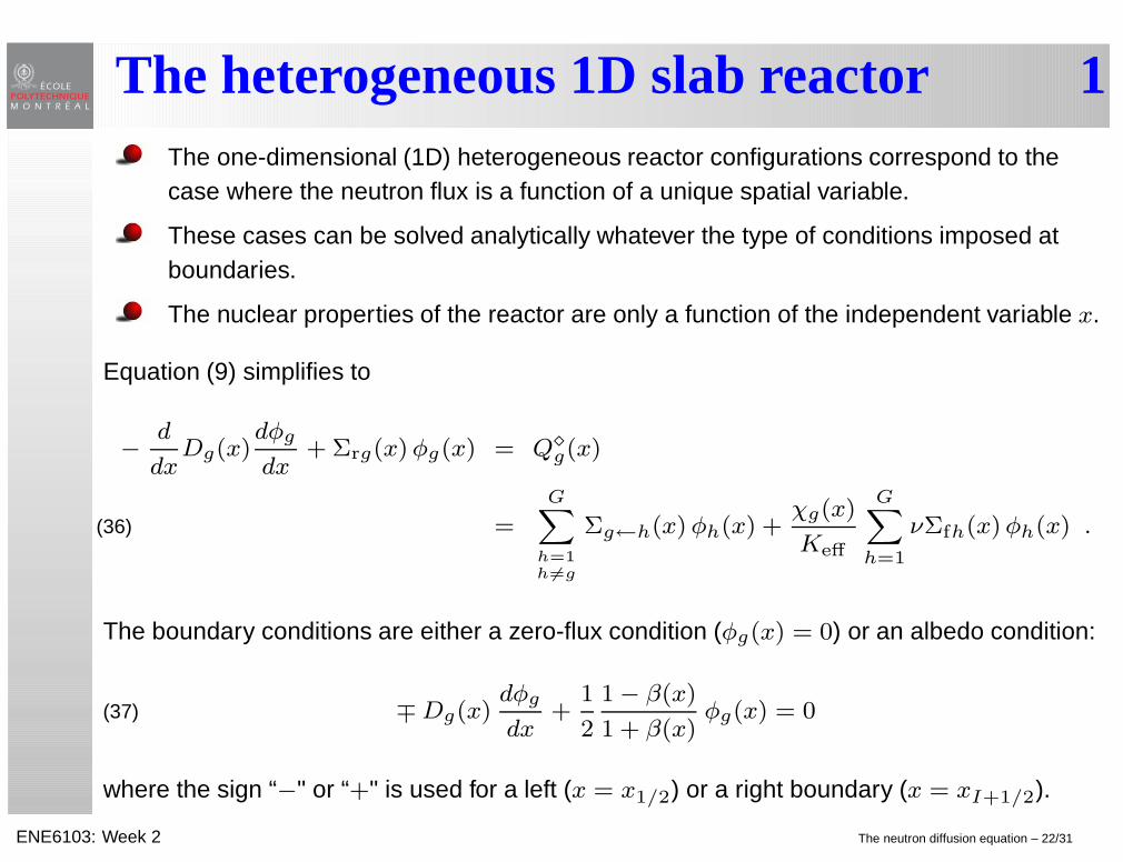
The heterogeneous 1D slab reactor 1The one-dimensional (1D) heterogeneous reactor configurations correspond to thecase where the neutron flux is a function of a unique spatial variable.
These cases can be solved analytically whatever the type of conditions imposed atboundaries.
The nuclear properties of the reactor are only a function of the independent variable x.
Equation (9) simplifies to
−d
dxDg(x)
dφg
dx+ Σrg(x)φg(x) = Q⋄g(x)
=
GX
h=1
h6=g
Σg←h(x)φh(x) +χg(x)
Keff
GX
h=1
νΣfh(x)φh(x) .(36)
The boundary conditions are either a zero-flux condition (φg(x) = 0) or an albedo condition:
∓Dg(x)dφg
dx+
1
2
1 − β(x)
1 + β(x)φg(x) = 0(37)
where the sign “−" or “+" is used for a left (x = x1/2) or a right boundary (x = xI+1/2).
ENE6103: Week 2 The neutron diffusion equation – 22/31

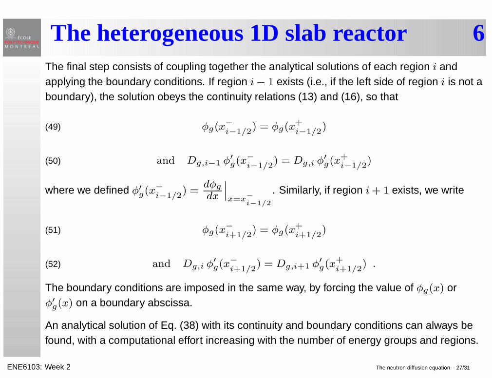
The heterogeneous 1D slab reactor 2
Each slab is assumed to be homogeneous, so that the corresponding nuclear propertiesDg(x), Σrg(x), Σg←h(x), χg(x) and νΣfh(x) are piecewise continuous. The reactordomain is divided into I regions of indices 1 ≤ i ≤ I, in such a way that the nuclearproperties in region i are constant and equal to Dg,i, Σrg,i, Σg←h,i, χg,i and νΣfh,i.
i-1 i i+1
xi-3/2 xi-1/2 xi+1/2 xi+3/2
xi-1 xi+1 xi
∆xi-1 ∆xi ∆xi+1
X
region regionregion
Equation (36) can be written in such a way as to be valid in region i as
−Dg,id2φg
dx2+ Σrg,i φg(x) = Q⋄g(x) =
GX
h=1
h6=g
Σg←h,i φh(x) +χg,i
Keff
GX
h=1
νΣfh,i φh(x)
if xi−1/2 < x < xi+1/2 .(38)
ENE6103: Week 2 The neutron diffusion equation – 23/31

The heterogeneous 1D slab reactor 3At this point, we introduce the analytical solution approach for Eq. (38). It is based on alinear transformation technique, valid only for multigroup 1D problems. Equation (38) is firstrewritten in matrix form as
d2
dx2Φ(x) + FiΦ(x) = 0 if xi−1/2 < x < xi+1/2(39)
with
Φ(x) =
0
B
B
@
φ1(x)
...φG(x)
1
C
C
A
and Fi =
0
B
B
B
B
@
f11,i f12,i . . . f1G,i
f21,i f22,i . . . f2G,i
......
. . ....
fG1,i fG2,i . . . fGG,i
1
C
C
C
C
A
(40)
where the components fgh,i of this matrix are written as
fgh,i =1
Dg,i
»
−Σrg,iδgh + Σg←h,i(1 − δgh) +χg,i
Keff
νΣfh,i
–
.(41)
ENE6103: Week 2 The neutron diffusion equation – 24/31

The heterogeneous 1D slab reactor 4The next step consists in finding all eigenvectors tℓ,i of matrix Fi with the associatedeigenvalues λℓ,i. We build a matrix Ti whose columns are the eigenvectors of Fi:
Ti = ( t1,i t2,i . . . tG,i )(42)
so that
Fi Ti = Tidiag(λℓ,i) .(43)
The linear transformation technique used to solve Eq. (36) is based on the introduction of anunknown vector Ψ(x) defined in such a way that
Φ(x) = TiΨ(x) =
0
B
B
B
B
@
t11,i t12,i . . . t1G,i
t21,i t22,i . . . t2G,i
......
. . ....
tG1,i tG2,i . . . tGG,i
1
C
C
C
C
A
0
B
B
B
B
@
ψ1(x)
ψ2(x)
...ψG(x)
1
C
C
C
C
A
(44)
and to its substitution in Eq. (39). We obtain
d2
dx2Ti Ψ(x) + Fi Ti Ψ(x) = 0 if xi−1/2 < x < xi+1/2 .(45)
ENE6103: Week 2 The neutron diffusion equation – 25/31

The heterogeneous 1D slab reactor 5We next left–multiply each side of Eq. (45) by [Ti]
−1 and use Eq. (43) to obtain
d2
dx2Ψ(x) + diag(λℓ,i)Ψ(x) = 0 if xi−1/2 < x < xi+1/2 .(46)
Equation (46) is similar to Eq. (39) with the difference that all the energy groups areuncoupled. Its resolution is reduced to the solution of G one-speed problems. In eachenergy group g, we assume an analytical solution of the form
ψg(x) =
8
>
<
>
:
Ag,i cos(p
λg,i x) + Bg,i sin(p
λg,i x) if λg,i ≥ 0;
Cg,i cosh(p
−λg,i x) + Eg,i sinh(p
−λg,i x) otherwise(47)
if xi−1/2 < x < xi+1/2.
The analytical expression of the flux φg(x) is obtained after substitution of Eq. (47) intoEq. (44) as
φg(x) =
GX
h=1
tgh,i ψh(x) if xi−1/2 < x < xi+1/2 .(48)
ENE6103: Week 2 The neutron diffusion equation – 26/31
The heterogeneous 1D slab reactor 6The final step consists of coupling together the analytical solutions of each region i andapplying the boundary conditions. If region i− 1 exists (i.e., if the left side of region i is not aboundary), the solution obeys the continuity relations (13) and (16), so that
φg(x−i−1/2
) = φg(x+
i−1/2)(49)
and Dg,i−1 φ′
g(x−i−1/2
) = Dg,i φ′
g(x+
i−1/2)(50)
where we defined φ′g(x−i−1/2
) =dφg
dx
˛
˛
˛
x=x−i−1/2
. Similarly, if region i+ 1 exists, we write
φg(x−i+1/2
) = φg(x+
i+1/2)(51)
and Dg,i φ′
g(x−i+1/2
) = Dg,i+1 φ′
g(x+
i+1/2) .(52)
The boundary conditions are imposed in the same way, by forcing the value of φg(x) orφ′g(x) on a boundary abscissa.
An analytical solution of Eq. (38) with its continuity and boundary conditions can always befound, with a computational effort increasing with the number of energy groups and regions.
ENE6103: Week 2 The neutron diffusion equation – 27/31

Two-region example 1We apply this technique to a one-speed,two-region problem. Eq. (38) simplifies to
−Did2φ
dx2+ Σr,i φ(x) =
1
Keff
νΣf,i φ(x)
if xi−1/2 < x < xi+1/2 .(53)
0 1/2 1
C L
X
region 1 region 2
zero
-flu
x
We assume an analytical solution of the form
φ(x) =
8
>
<
>
:
A11 cos(κ1x) +A21 sin(κ1x) if 0 ≤ x ≤ 1
2;
A12 cos(κ2x) +A22 sin(κ2x) if 1
2≤ x ≤ 1
(54)
φ′(x) =
8
>
<
>
:
−A11 κ1 sin(κ1x) + A21 κ1 cos(κ1x) if 0 ≤ x ≤ 1
2;
−A12 κ2 sin(κ2x) + A22 κ2 cos(κ2x) if 1
2≤ x ≤ 1
(55)
d2φ
dx2=
8
>
<
>
:
−A11 κ21 cos(κ1x) −A21 κ
21 sin(κ1x) if 0 ≤ x ≤ 1
2;
−A12 κ22 cos(κ2x) −A22 κ
22 sin(κ2x) if 1
2≤ x ≤ 1 .
(56)
ENE6103: Week 2 The neutron diffusion equation – 28/31

Two-region example 2The left zero-flux boundary condition is written
φ(0) = A11 = 0 .(57)
The continuity conditions at x = 1
2are written
A11 cos“κ1
2
”
+A21 sin“κ1
2
”
= A12 cos“κ2
2
”
+A22 sin“κ2
2
”
(58)
and
−A11 κ1D1 sin“κ1
2
”
+A21 κ1D1 cos“κ1
2
”
= −A12 κ2D2 sin“κ2
2
”
+A22 κ2D2 cos“κ2
2
”
.
(59)
Finally, the right symmetry boundary condition is written
−A12 κ2 sin(κ2) +A22 κ2 cos(κ2) = 0
so that
A22 = A12 tan(κ2) .(60)
ENE6103: Week 2 The neutron diffusion equation – 29/31
Two-region example 3Substituting Eqs. (57) and (60) into Eqs. (58) and (59), we find the following matrix equation:
0
B
@
sin`κ1
2
´
−1
cos(κ2)cos“κ2
2
”
κ1D1 cos`κ1
2
´
−κ2D2
cos(κ2)sin“κ2
2
”
1
C
A
„
A21
A12
«
=
„
0
0
«
.(61)
Equation (61) has a non-trivial solution only if its determinant is zero. We write
det
0
B
@
sin`κ1
2
´
−1
cos(κ2)cos“κ2
2
”
κ1D1 cos`κ1
2
´
−κ2D2
cos(κ2)sin“κ2
2
”
1
C
A= 0(62)
so that the resulting characteristic equation is a non-linear relation in κ1 and κ2, written
tan“κ1
2
”
tan“κ2
2
”
=κ1D1
κ2D2
.(63)
Substituting Eqs. (54) and (56) into Eq. (53), we find the expressions of κ1 and κ2 as
κ1 =
s
νΣf,1 −KeffΣr,1
KeffD1
and κ2 =
s
νΣf,2 −KeffΣr,2
KeffD2
.(64)
ENE6103: Week 2 The neutron diffusion equation – 30/31
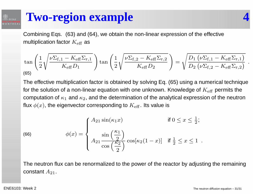
Two-region example 4Combining Eqs. (63) and (64), we obtain the non-linear expression of the effectivemultiplication factor Keff as
tan
1
2
s
νΣf,1 −KeffΣr,1
KeffD1
!
tan
1
2
s
νΣf,2 −KeffΣr,2
KeffD2
!
=
s
D1
`
νΣf,1 −KeffΣr,1
´
D2
`
νΣf,2 −KeffΣr,2
´ .
(65)
The effective multiplication factor is obtained by solving Eq. (65) using a numerical techniquefor the solution of a non-linear equation with one unknown. Knowledge of Keff permits thecomputation of κ1 and κ2, and the determination of the analytical expression of the neutronflux φ(x), the eigenvector corresponding to Keff . Its value is
φ(x) =
8
>
>
>
>
<
>
>
>
>
:
A21 sin(κ1x) if 0 ≤ x ≤ 1
2;
A21
sin“κ1
2
”
cos“κ2
2
” cos[κ2(1 − x)] if 1
2≤ x ≤ 1 .
(66)
The neutron flux can be renormalized to the power of the reactor by adjusting the remainingconstant A21.
ENE6103: Week 2 The neutron diffusion equation – 31/31


![Service de Metrologie Nucl´ eaire´ - [Groupe Calcul]calcul.math.cnrs.fr/IMG/pdf/aggamgtut_notay.pdf · Aggregation-based algebraic multigrid A tutorial Yvan Notay∗ Universite](https://static.fdocuments.us/doc/165x107/5ac819857f8b9aa3298bbf47/service-de-metrologie-nucl-eaire-groupe-calcul-algebraic-multigrid-a-tutorial.jpg)


