2004-01-1418

Instantaneous Exhaust Temperature Measurements Using Thermocouple Compensation Techniques

Kenneth Kar, Stephen Roberts, Richard Stone, Martin Oldfield University of Oxford

Boyd French Ford Motor Company

Copyright © 2003 SAE International

ABSTRACT

This paper discusses a method of measuring the instantaneous exhaust gas temperature by thermocouples. Measuring the exhaust gas temperature is useful for a better understanding of engine processes. Thermocouples do not measure the instantaneous exhaust gas temperature because of their limited dynamic response. A thermocouple compensation technique has been developed to estimate the time constant in situ. This method has been commissioned in a simulation study and a controlled experiment with a reference temperature. The studies have shown that the signal bandwidth has to be restricted, since noise will be amplified in the temperature reconstruction. The technique has been successfully applied to some engine exhaust measurements. A comparison between two independent pairs of thermocouples has shown that temperature variations at frequencies up to 80Hz can be recovered. The medium load results agree with a previous study, which used fast response thermometers with a bandwidth of about 50 Hz. However, the results at low load and two different speeds have highlighted the need to do some 1-D unsteady flow simulations, in order to gain more insight into the exhaust process.

INTRODUCTION

With the introduction of even more stringent emission limits (EURO IV, SULEV), engine developers are striving to better understand engine processes. Exhaust gas temperature (EGT) can be very useful in this respect. For instance, the heat transfer across the exhaust port can be estimated with EGT measurements, and this would enable a better heat transfer model to be developed. In addition, EGT forms the basic calibration data for computational fluid dynamic models (CFD), which are commonly used in engine design.

Knowing the exhaust gas temperature can immediately help many other applications as well. Following the engine cold start, the catalytic converter has not yet reached its operating temperature, so most of the

hydrocarbon emissions are untreated. A study has suggested that more than 80% of the hydrocarbon emission measured over the entire FTP-75 drive cycle are emitted within the first 20 seconds after the engine has started [1]. The performance of the catalyst can be optimized if the EGT is known. This should have an immediate improvement on hydrocarbon emissions. Performance wise, using EGT as the control input, there is a scope for active exhaust control as the propagation velocity of the pressure waves is closely related to EGT [2]. Lastly, the performance of a turbocharger may be enhanced since its operating point can be accurately determined with instantaneous exhaust temperature measurements, especially when it is subject to a fluctuating exhaust flow.

There are a range of thermometers available to measure exhaust gas temperature. The most commonly used is the thermocouple because of its low cost, simplicity and the wealth of experience in their application. However, because of their slow response (typically 0.1 Hz to 5 Hz), they are only used for measuring time-averaged temperatures. Ideally the instantaneous temperature is needed, so that transient phenomenon can be observed. Other thermometers have been applied in engine diagnostics such as the acoustic technique [3], optical (laser) diagnostics [4, 5] and resistance thermometry [6, 7]. Their responses certainly meet the requirements and may exceed them in many cases. However, they tend to be complicated, difficult to set up and maintain, and so are generally expensive. Only a limited number of people and laboratories would have access to them. It is unlikely that such systems will become so economical that they are as popular as some well established thermometers, like thermocouples.

For exhaust gas temperature measurement, the frequencies of interest are mostly below 100 Hz. In fact this is not a very demanding situation. Opting for the above fast response systems may not be a cost effective solution. Instead, trying to improve the performance of thermocouples would be desirable. Now it is possible that the response of thermocouples may be improved by

some novel compensation techniques. In this case, the total cost of the measuring system would not increase much, as no additional hardware is required. All the technology and equipment developed for thermocouples can still be used. This technology will have much wider applications than the existing system, and yet have an acceptable response (~100 Hz).

The response of thermocouples along with the various compensation techniques will be presented here. A new method will be proposed to overcome the previous shortcomings. This method will be validated by simulation and a controlled experiment. Finally, the application of this method is demonstrated by showing exhaust temperature measurements from a spark-ignition engine.

DYNAMIC RESPONSES

By performing an energy balance, the dynamic response of a thermocouple can be described by Eq. 1.

( )4surr

4w

w2w

2wwww

wg 44TT

hxT

hdk

tT

hdcTT −+

∂∂

−∂

∂=−

σερ (1)

The above analysis has assumed that the temperature distribution of any cross section of the thermocouple wire is uniform at any instant. In this paper, the Biot number of the largest thermocouple is in the order of 3e-3, which is much smaller than 0.1, so this assumption is justified.

Eq. 1 states that the difference between the gas temperature (Tg) and the wire temperature (Tw) is due to three effects, as shown by the three terms on the RHS. The first term is the dynamic error. Because the thermocouple wire has a finite mass, its temperature cannot follow the changes in gas temperature instantaneously. The second term is the conduction error: the probe support will generally respond to the change in gas temperature more slowly than the wire, so a temperature gradient will exist between the wire and the support, and heat will conduct from or to the wire. The last term is the radiation error. The surroundings are normally much colder than the thermocouple, so heat will radiate from the thermocouple to the surrounding. If conduction and radiation are negligible, Eq. 1 can be reduced to

tTTTd

d wwg τ=− (2)

where, hdc 4wwρτ = . Eq. 2 is a first-order ordinary differential equation, completely characterized by τ. Even in the presence of conduction and radiation, Scadron and Warshawshy [8] have shown that the thermocouple response still behaves like a first-order system, which can be described by

tTTTd

~d~~ w*wg τη =− (3)

where: the tilde denotes the fluctuation about the mean temperature, η is the ratio of equilibrium thermocouple reading to the reading it would give if it were at the true temperature, and τ* is the time constant which has the conduction and radiation effect taken into account.

TEMPERATURE RECONSTRUCTION

RESPONSE EQUATION

In exhaust gas measurements, what is of interest is the instantaneous gas temperature (Tg). If τ* and η are known, Eq. 2 or Eq. 3 can be solved for Tg; η may be calculated from a know radiation and conduction correction factor [8]. Otherwise the thermocouple is designed to minimize conduction and radiation errors, so η is close to unity. The Conduction and Radiation section will show that η is close to unity, so the main task here is to find the time constant.

PREVIOUS WORK

It is very difficult to find the time constant analytically for the following reasons:

• Nusselt correlations are derived for steady flow conditions.

• Some fluid and material properties are strong functions of temperature

• The time constant is a function of radiation and conduction parameters.

In an engine exhaust, the flow is unsteady with large temperature variations (of the order 500 K). In addition, chemical reactions (post oxidation of the burnt gas) might still be taking place. Therefore, early research concentrated on empirical methods. The time constant can be measured by exposing the thermocouple to the test flow. If an electric current is then passed through the thermocouple, creating a step change in temperature, then by observing the temperature decay, the time constant is the time required for the junction temperature to decrease to 63.2% of the difference between the initial and the final temperatures. This method can only give an average time constant for a particular flow condition. So, the accuracy of the reconstruction will depend on how much the flow changes. In an engine exhaust, the flow will be almost stagnant when the exhaust valve is closed, but it will be at very high speed during blowdown. Therefore, this method is unsuitable. Later developments have been with 2-thermocouple techniques. Many techniques have been proposed, but they are all based on the same principle. If two thermocouples are placed in close proximity, they will be exposed to the same temperature and velocity fields. It follows that by utilizing this fact, with additional assumptions, the time constants can be estimated in

situ. Denoting subscript 1 and 2 for thermocouples 1 and 2 respectively, the response equations are:

=+=

=+=

gw2

2w2g2

gw1

1w1g1

ddd

d

TtTTT

TtTTT

τ

τ (4)

There are 3 unknowns with 2 equations. Cambray [9] introduced a constant time-constant ratio (α) to solve Eq. 4. If the heat transfer between the gas and the thermocouple is dominated by convection and the temperature dependence of the material properties of the thermocouple is weak, it can be shown that:

m

dd

−

==

2

1

2

1

2

ττα (5)

where: d is the diameter of the junction and m is the coefficient of the Reynolds number in the Nusselt correlation. Eq. 4 can then be rearranged and solved for τ1 as

( )

tTtTTT

/dd/dd 21

211 α

τ−

−−= (6)

This method gives the instantaneous time constant, but it can be shown to be highly susceptible to noise. Consider Eq. 7 below:

( )

den21

num211 /dd/dd etTtT

eTT+−

+−−=

ατ (7)

In a noiseless case when the denominator is approaching zero, the numerator is also approaching zero, so there is no singularity. However, if noise enum and eden are present, enum will be amplified when the denominator is approaching zero. Because the denominator also contains noise, the equation is ill defined over a region. The result is erratic with unphysical time constants, rendering the temperature reconstruction erroneous. Forney and Fralick [10] tried to tackle the noise problem by working in the frequency domain, such that

( )

12

212g1g

1TTTTTT

−−

==αα

(8)

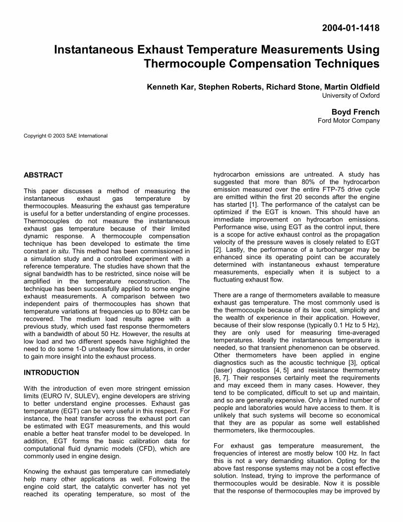
where, the overbar denotes a discrete Fourier transform (DFT) of the respective quantities. In this method, the gas temperature is found directly, bypassing the step of finding the time constants. Unfortunately, O’Reilly, et. al. [11] later discovered that noise can drive Eq. 8 to a singularity. When this occurs, the reconstructed gas temperature exhibits large amplitude oscillations as shown in Figure 1.

Figure 1 Comparison of the true and the reconstructed gas temperature using frequency domain technique (O’Reilly, et. al. [11])

Recall that Eq. 4 can be solved if either an additional criterion or information is introduced. So far the techniques have been based on assuming a constant time-constant ratio, which is susceptible to noise. Other criteria are possible, such as the Least-Squares method first proposed by Tagawa and Ohta [12]. They argued that the two thermocouples in practice may not sense the same temperature because of dust contamination and spatial errors. Also, in the process of reconstruction, noise in the thermocouple signals will prevent the two gas temperatures being equal. Instead they sought to minimize the difference over a time window of N samples, which is given by:

( )∑=

−=N

i

ii TTN 1

2)(g2

)(g1

1ξ (9)

where the superscript i indicates the ith sample of the digitized data. Eq. 9 is minimized when

0;021

=∂∂

=∂∂

τξ

τξ

(10)

The two extra equations enable the time constants to be determined without a priori a time-constant ratio. With noisy signals, this method may sometimes give negative time constants, which are physically impossible. This may be explained by considering Eq. 4. The τ1dTw1/dt and τ2dTw2/dt terms represent the dynamic errors of the thermocouples at any time. The least-squares criterion only considers a difference in Tg (Eq. 9), and this can be influenced by the time constants and/or the gradients. In other words, it is a conditional minimization procedure, dependent upon what gradients are given. Unfortunately, it can be shown that noise in the signals can be over-amplified when numerical gradients are evaluated. This will be discussed further later. Therefore if the gradients have been amplified, the least-squares method would try to make a correction by giving a negative time constant, since negative time constants have the effect of attenuation.

Several improvements have been proposed by various researchers such as:

• Correlation coefficient [13] — this method is based on the assumption that noise has no correlation. By using the correlation coefficient as the criterion, it should better discriminate the signal from the noise.

• Frequency domain [14] — this method equates the two reconstructed temperatures in the frequency domain. This would allow filtering to be applied easily. At the same time this method restricts the bandwidth of the reconstruction by only considering the spectrum up to a certain frequency.

• Constant time-constant ratio [2] — the least squares method is prone to noise and can give negative time constants. By reintroducing the constant time-constant ratio assumption, it reduces one order of freedom in the equations, making this method less likely to give negative time constants.

• Total Least Squares [15] — the response equations (Eq. 4) are described by difference equations to form an autoregressive (ARX) model with noise added in the input as well as in the output. The parameters of the ARX model are related to the time constants, and can be estimated by the Total Least Squares. Theoretically the Total Least Squares will give unbiased estimates when the noise variances on the input and output are equal.

All these improvements aim to handle the noise better, so as to get an unbiased estimate of the time constants. However, one serious limitation remains, that is the least squares method processes the data in a time window. Within each window, the time constants are assumed to be constant. The size of the window (N in Eq. 9) is found to be a compromise between temporal resolution and accuracy [16]. Tagawa and Ohta [12] recommended that the window should have a duration of at least 1.5 times longer than the mean time constant of the smaller thermocouple. Yet, ideally the window size should accommodate the dynamics of the system. For example during blowdown, a short window size should be used compared to the time when the exhaust valve is closed. Above all, without knowing the gas temperature, it is difficult to find the optimal window duration for the reconstruction. O’Reilly [11] overcame this limitation by a nonlinear state estimator — the Extended Kalman Filter (EKF). The thermocouple model is written in a state-space model with the constant time-constant ratio assumption. The gas temperatures (Tg) and the time constant (τ) being the states, are estimated simultaneously and recursively, so there is no time window to be set. The model itself is stochastic in nature, allowing explicitly for noise on the signals. However it also means that the dynamic of the states, in particular Tg and τ are governed by the noise covariances, which have to be specified a priori. Because the EKF works by linearizing the states about the current states estimate, it is a perturbation model. Unsuitable initial conditions and covariances may lead to stability problems. Simulation experience has shown the covariance on τ has a great impact on stability. There are a total of six parameters;

without a reference thermometer, there is no guideline as to how to tune these six parameters, since their effects on accuracy are not known. An alternative Kalman filter has been developed here. It has all the advantages of the EKF, plus the following:

• No a priori assumptions for the time constant ratio • The covariances are to be inferred from the data,

thereby eliminating any subjective tuning (see the Estimation of noise parameters section).

• The two reconstructed temperatures may differ. This flexibility makes it less susceptible to noise (unlike the constant time-constant method).

• The accuracy of the estimation is quantified, and provided to the user.

This is to the authors’ knowledge the most versatile method available. Table 1 compares the various methods in terms of the assumptions made.

Table 1 Assumptions in the different methods for time constant estimation

Method Tg1 = Tg2 Constant τ Constant α Cambray Yes No Yes Forney and Fralick

Yes Yes Yes

Tagawa and Ohta

No Yes No

O’Reilly et. al. No No Yes Kalman filter No No No

KALMAN FILTER

The Kalman filter is a recursive procedure for estimating the latent variables, θ, in the following linear stochastic equation [17].

)()()()(

)()1()()(

iiii

iiii

vθFywθGθ

+=

+= −

(11)

where:

G is a flow matrix

w is the state noise, normally distributed with zero mean and covariance W.

y are the multivariate observations

F is a transformation matrix

v is the observation noise, normally distributed with zero mean and covariance matrix V.

TIME CONSTANT FORMULATION

The latent variables of interest are the time constants τ1 and τ2. To use the Kalman filter, the flow matrix, which describes how τ1 and τ2 vary with time, has to be defined. This requires knowledge of the system dynamics of the time constants (a mathematical model). As discussed before, this would be very difficult. The best alternative is to assume G = I, which means that the most likely values in the next time step are the same as the present values. It would be the noise, w that allows the time constants to change over time. It will be shown later on how this noise can be estimated. This assumption will simplify the application of the Kalman filter to a Dynamic Linear Model [17] as,

)()()()(

)()1()(

iiii

iii

vθFywθθ+=

+= −

(12)

Eliminating Tg in Eq. 4 and rearranging gives

tT

tTTT

dd

dd w2

2w1

1w2w1 ττ +−=− (13)

Eq. 13 can be written into Matrix-Vector form for the ith time step as

−=− )(

2

)(1

)(2

)(1w)(

2)(

1w dd

dd

i

iiw

iiw

i

tT

tTTT

ττ

(14)

By comparing Eq. 14 against Eq. 12, it can be seen that Eq. 14 is a Dynamic Linear Model with:

• A univariate observation, y = Tw1 – Tw2 • The two time constants (τ1 and τ2) as the latent

variables, θ • The gradients defining the transformation matrix, F Because the observation is univariate, only a scalar σ2 is required to describe the observation noise, v.

RECURSIVE ESTIMATION

The latent variables can then be estimated with the following recursive formulae

)()()()()(

)()()1()( ˆˆiiiii

iiii eRFKRΣ

Kθθ−=

+= −

(15)

where:

)(iΣ is the covariance of the latent variables,

( )( ) )(2

ˆ

)(T)()(

iy

iii

σFRK = , is the Kalman gain matrix,

)()1()( iii WΣR += − , is the covariance of the latent variables prior to y(i) being observed,

( ) ( ) ( ) )(2)(2)(2ˆ

iiiy θσσσ += , is the estimated prediction

variance, and is composed of two terms: the observation noise variance, σ2 and the component of prediction variance due to uncertainty in the latent variables, 2

θσ . It

is given by ( ) ( ) )(T)()()(2 iiii FRF=θσ ,

)()()( ˆ iii yye −= , is the prediction error, and

)1()()( ˆˆ −= iiiy θF , is the prediction.

A useful quantity is the likelihood of an observation, given the model parameter before they are updated is given by:

( ) ( )( ))(2ˆ

)()( ,ˆ iy

ii yNyp σ= (16)

In Bayesian terminology this likelihood is known as the evidence for the data point. It will be used for estimation of the observation noise, σ2.

ESTIMATION OF NOISE PARAMETERS

State noise

The noise parameter is estimated by Jazwinski’s method [18]. The state noise covariance matrix is assumed to be an isotropic matrix, W = qI. The prediction variance (σq0

2) is calculated, assuming no state noise, i.e. q = 0 by:

( ) ( ) ( ) )(T)1()()(2)(20

iiiiiq FΣF −+= σσ (17)

If σq02 is smaller than the prediction error (e2), the state

noise is inferred to be non-zero. This logic can be implemented using a ramp function in Eq. 18.

≥

=otherwise0

0 if)(

K

K xxxh (18)

Therefore, q can be updated according to:

( ) ( )

( )

−= )(T)(

)(20

)(2)(

ii

iq

ii ehq

FF

σ (19)

Observation noise

Eq. 15 shows that the estimated prediction variance is made up of the observation noise and the component due to the uncertainty in the latent variables. Thus the observation noise can be estimated by subtracting the second component from the prediction error as

( ) ( ) ( )( ))(T)1()()(2)(2 iiiii eh FRF −−=σ (20)

It can be proved that the observation noise estimated by Eq. 20 will maximize the likelihood of the observation in the next sample (Eq. 16).

EQUIPMENT

THERMOCOUPLE PROBE

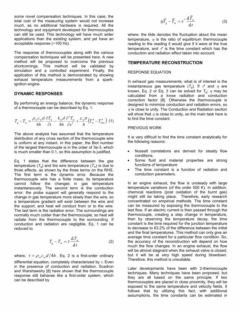
A schematic diagram showing the main features of the probe design is given in Figure 2. The thermocouple probe is 100 mm long, and 3 mm in diameter. It comprises of three main components:

1. Unsheathed fine gauge K type thermocouples, 2. Ceramic and stainless steel tubes, 3. Electrical socket and collet sets.

In this project, three pairs of bead-type thermocouples with wire diameters ranging from 50 to 127 µm (0.002” to 0.005”) were used. This gives 3 independent thermocouple pairs for comparison. With their different sensor sizes, the effects of: the signal-to-noise ratio, conduction and radiation, and the time-constant ratio can be investigated. For the compensation technique to be valid, the three thermocouples have to be close enough so that the measured volume is sufficiently small compared to the characteristic length scales of the thermal fields being investigated [12]. Therefore, the three thermocouples were densely packed, being about 500 µm apart.

The thermocouples were soldered into a seven-way LEMO socket, and this forms additional thermocouple junctions. An independent thermocouple is therefore needed to measure the junction temperature for cold-junction compensation.

100

4 STAINLESSSTEEL TUBE

LEMO 7-WAYSOCKET

CERAMIC 6-BORE TUBE

REFERENCEJUNCTIONTHERMOCOUPLE

CHROMELALUMELCOPPER NOT TO SCALE

KEYS:

3

Figure 2 Schematic diagram of the thermocouple probe

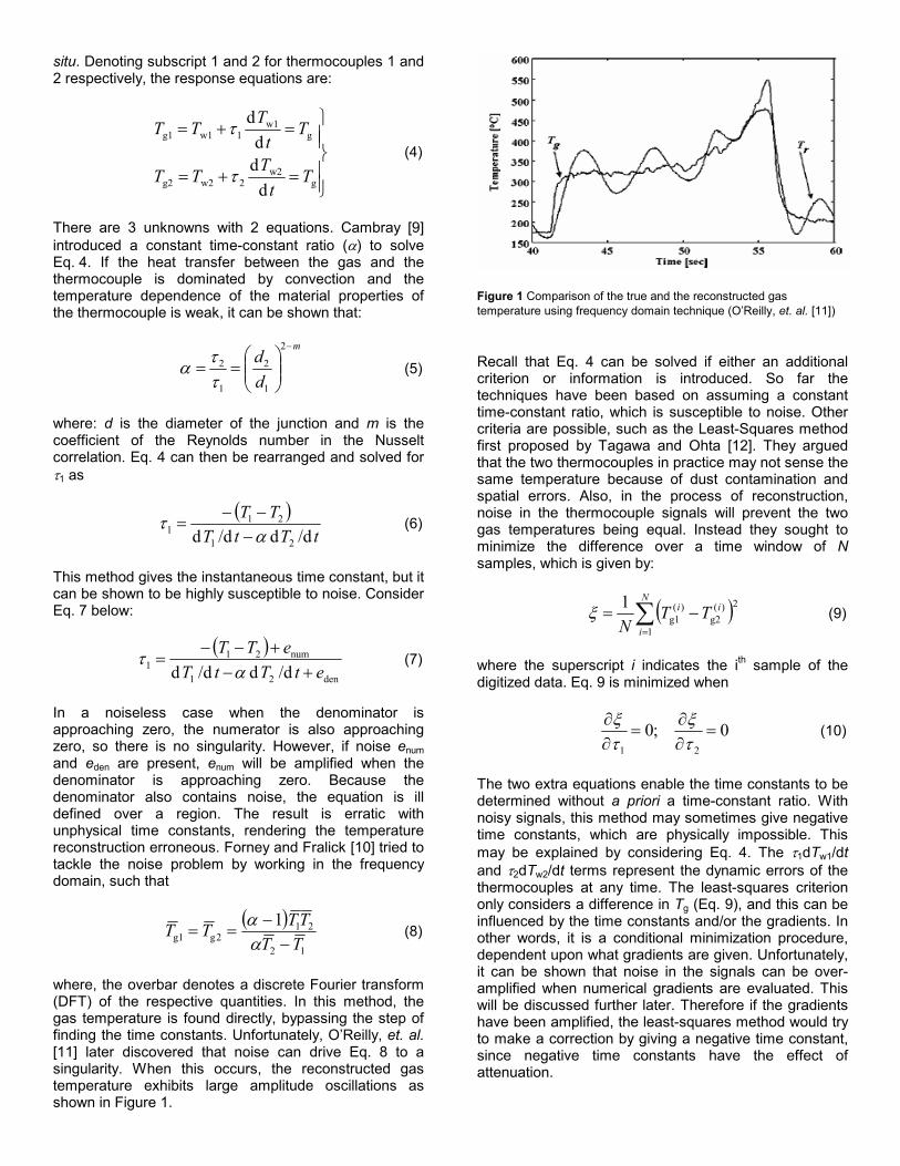
AIR TEST RIG

The thermocouples were tested in a well-controlled environment before the engine exhaust temperature experiments. A special air rig was set up as shown in Figure 3. There are two hot air guns supplying hot and cold air to a mixing valve. Within the valve, a shutter is revolving, and admitting hot and cold air alternately. The air is then mixed and accelerated through the nozzle at the outlet. The air rig is able to create temperature fluctuation from 90 to 120°C, at up to 200 Hz.

HOT STREAMCOLD STREAM

ADAPTOR HOT AIRGUN

NOZZLE

3-WAYVALVE

SHUTTER

Figure 3 Schematic diagram of the air rig

To validate the Kalman filter model, the instantaneous air temperature at the outlet was measured by a reference thermometer. The reference thermometer is a hot wire anemometer system using a two-wire technique in constant temperature mode [19]. With dual wires, velocity and temperature can be measured simultaneously. For the test conditions, the bandwidth of the reference system was in excess of 30 kHz, which far exceeded the temperature frequency that the air rig can produce. Unfortunately, the hot wire system is too fragile to be used in the engine exhaust directly.

ENGINE AND EXHAUST

The thermocouple probe was installed in the exhaust pipe of a production-type, spark ignition engine. It has 4 cylinders with a swept volume of 1396 cm3. The engine specification is summarized in Table 2 [20].

Table 2 Specification of the test engine

Bore (mm) 75.0 Stroke (mm) 79.0 Compression ratio 10.5 Maximum bmep (bar) 11.2 @ 3500 rpm Inlet valve opens (°btdc) 12 Inlet valve closes (°abdc) 52 Exhaust valve opens (°bbdc) 52 Exhaust valve closes (°atdc) 12

This study is concentrated on the 4th cylinder of the engine. The positions of various instruments are given in Figure 4. The thermocouple junctions are along the exhaust pipe’s centerline. There is a piezoresistive pressure transducer, about 27 mm upstream of the thermocouple. Both of them are about 100 mm away from the mean centre of the exhaust valves. The cylinder

and the inlet manifold pressures were also measured. To gauge the effect of radiation, a thermocouple was mounted on the external surface of exhaust pipe. Since the largest thermal resistance from the exhaust gas to the surrounding is the convection to and from the metal, there should be little difference between the internal and external surface temperatures. Moreover, a previous study on the instantaneous in-cylinder temperature suggested that there is only a 10 K temperature swing in a 4-stroke cycle of a firing engine [21]. Hence the temperature swing in the surface temperature of the exhaust would be even less; therefore the dynamic error in the exhaust pipe surface thermocouple can be ignored.

Figure 4 Schematic diagram showing how the instruments are placed relative to the exhaust valves. Left hand diagram is a plan view. Right hand diagram is a cross-sectional elevation. All dimensions are in millimeters.

SIGNAL CONDITIONING AND DATA ACQUISITION

The thermocouple signals were amplified 200 times by fast-settling instrumentation amplifiers. To reduce the high frequency electrical noise, the amplified signals were passed through a passive low-pass filter with a -3 dB point at 13 kHz. Since the maximum frequency of interest would be at least 10 times smaller, the phase distortion and attenuation introduced by the filter should be minimal. As a further assurance, a high-speed spectral analysis was conducted on the thermocouple signals. The results are plotted in Figure 5. The power spectrum diminishes quickly and settles to -100 dB at about 500 Hz Above this frequency, the spectrum contains little power, indicating that no extraneous signal has been added to the thermocouple signal. Signals from other thermocouples show similar spectra.

Figure 5 Power spectral density of a raw thermocouple signal measuring exhaust temperature. Sampling frequency is 300 kHz.

Lastly, the signals were digitized by a computer-based data acquisition system and saved in a standard ASCII file for post analysis. The data was collected by multi-channel scanning, in which the clock rate was controlled by the TTL pulse of a shaft encoder which was coupled to the crankshaft. Samples were collected every 1 degree crank angle.

MODEL VALIDATION

To ensure the integrity of the temperature reconstruction, the Kalman filter was commissioned in a simulation study and a well-controlled experiment before being applied to the exhaust temperature measurements.

SIMULATION STUDY

A sinusoidal variation of the gas temperature was defined. It was then used for solving the two thermocouple temperatures by Eq. 4 with a common initial temperature. The time constants, which have mean values of 30 and 70 ms, were also defined to vary sinusoidally at 1/5 of the temperature frequency. The two synthetic thermocouple time series were contaminated by Gaussian noise with very small variance of 1e-8. The resulting gas and thermocouple temperature traces are plotted in Figure 6.

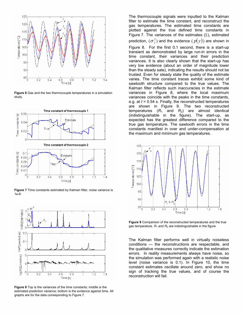
Figure 6 Gas and the two thermocouple temperatures in a simulation study.

Figure 7 Time constants estimated by Kalman filter, noise variance is 1e-8.

Figure 8 Top is the variances of the time constants; middle is the estimated prediction variance; bottom is the evidence against time. All graphs are for the data corresponding to Figure 7.

The thermocouple signals were inputted to the Kalman filter to estimate the time constant, and reconstruct the gas temperatures. The estimated time constants are plotted against the true defined time constants in Figure 7. The variances of the estimates (Σ), estimated prediction, ( 2

yσ ) and the evidence ( ( )yp ) are shown in Figure 8. For the first 0.1 second, there is a start-up transient as demonstrated by large run-in errors in the time constant, their variances and their prediction variances. It is also clearly shown that the start-up has very low evidence (about an order of magnitude lower than the steady sate), indicating the results should not be trusted. Even for steady state the quality of the estimate varies. The time constant traces exhibit some kind of sawtooth structure compared to the true values. The Kalman filter reflects such inaccuracies in the estimate variances in Figure 8, where the local maximum variances coincide with the peaks in the time constants, e.g. at t = 0.54 s. Finally, the reconstructed temperatures are shown in Figure 9. The two reconstructed temperatures (R1 and R2) are almost identical (indistinguishable in the figure). The start-up, as expected has the greatest difference compared to the true gas temperature. The sawtooth errors in the time constants manifest in over and under-compensation at the maximum and minimum gas temperatures.

Figure 9 Comparison of the reconstructed temperatures and the true gas temperature. R1 and R2 are indistinguishable in the figure

The Kalman filter performs well in virtually noiseless conditions — the reconstructions are respectable, and the qualitative measures correctly indicate the estimation errors. In reality measurements always have noise, so the simulation was performed again with a realistic noise level (noise variance is 0.1). In Figure 10, the time constant estimates oscillate around zero, and show no sign of tracking the true values, and of course the reconstruction will fail.

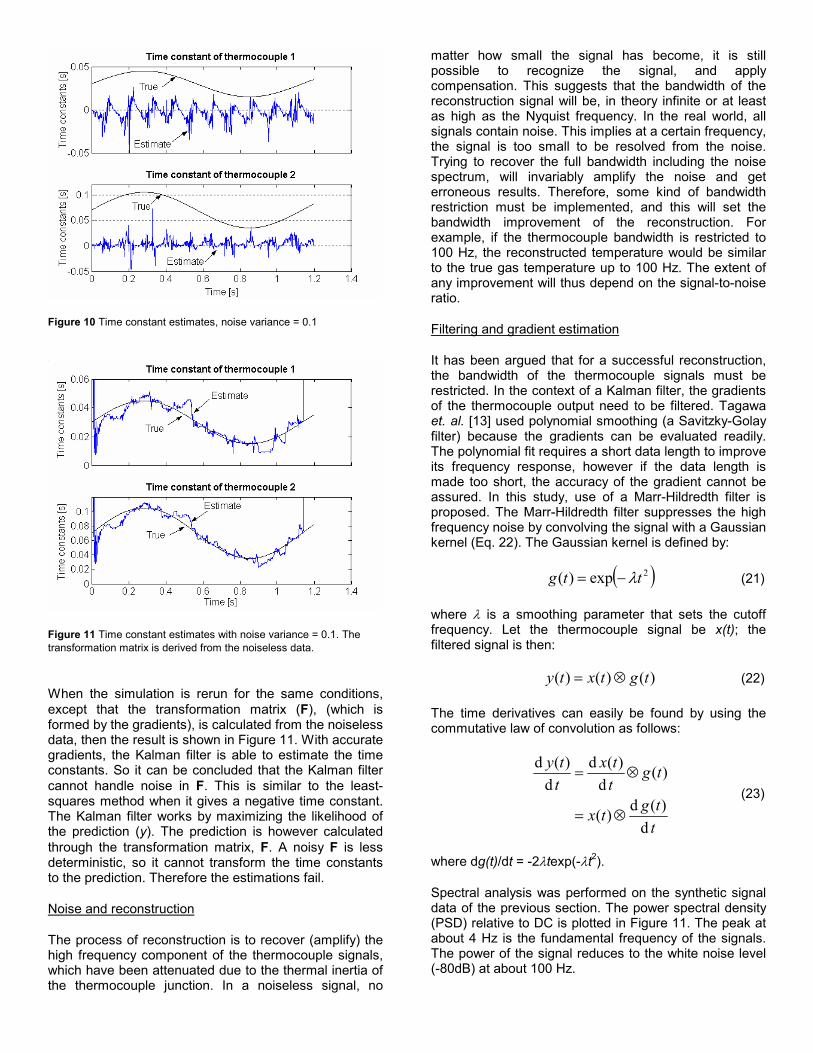
Figure 10 Time constant estimates, noise variance = 0.1

Figure 11 Time constant estimates with noise variance = 0.1. The transformation matrix is derived from the noiseless data.

When the simulation is rerun for the same conditions, except that the transformation matrix (F), (which is formed by the gradients), is calculated from the noiseless data, then the result is shown in Figure 11. With accurate gradients, the Kalman filter is able to estimate the time constants. So it can be concluded that the Kalman filter cannot handle noise in F. This is similar to the least-squares method when it gives a negative time constant. The Kalman filter works by maximizing the likelihood of the prediction (y). The prediction is however calculated through the transformation matrix, F. A noisy F is less deterministic, so it cannot transform the time constants to the prediction. Therefore the estimations fail.

Noise and reconstruction

The process of reconstruction is to recover (amplify) the high frequency component of the thermocouple signals, which have been attenuated due to the thermal inertia of the thermocouple junction. In a noiseless signal, no

matter how small the signal has become, it is still possible to recognize the signal, and apply compensation. This suggests that the bandwidth of the reconstruction signal will be, in theory infinite or at least as high as the Nyquist frequency. In the real world, all signals contain noise. This implies at a certain frequency, the signal is too small to be resolved from the noise. Trying to recover the full bandwidth including the noise spectrum, will invariably amplify the noise and get erroneous results. Therefore, some kind of bandwidth restriction must be implemented, and this will set the bandwidth improvement of the reconstruction. For example, if the thermocouple bandwidth is restricted to 100 Hz, the reconstructed temperature would be similar to the true gas temperature up to 100 Hz. The extent of any improvement will thus depend on the signal-to-noise ratio.

Filtering and gradient estimation

It has been argued that for a successful reconstruction, the bandwidth of the thermocouple signals must be restricted. In the context of a Kalman filter, the gradients of the thermocouple output need to be filtered. Tagawa et. al. [13] used polynomial smoothing (a Savitzky-Golay filter) because the gradients can be evaluated readily. The polynomial fit requires a short data length to improve its frequency response, however if the data length is made too short, the accuracy of the gradient cannot be assured. In this study, use of a Marr-Hildredth filter is proposed. The Marr-Hildredth filter suppresses the high frequency noise by convolving the signal with a Gaussian kernel (Eq. 22). The Gaussian kernel is defined by:

( )2exp)( ttg λ−= (21)

where λ is a smoothing parameter that sets the cutoff frequency. Let the thermocouple signal be x(t); the filtered signal is then:

)()()( tgtxty ⊗= (22)

The time derivatives can easily be found by using the commutative law of convolution as follows:

ttgtx

tgttx

tty

d)(d)(

)(d

)(dd

)(d

⊗=

⊗= (23)

where dg(t)/dt = -2λtexp(-λt2).

Spectral analysis was performed on the synthetic signal data of the previous section. The power spectral density (PSD) relative to DC is plotted in Figure 11. The peak at about 4 Hz is the fundamental frequency of the signals. The power of the signal reduces to the white noise level (-80dB) at about 100 Hz.

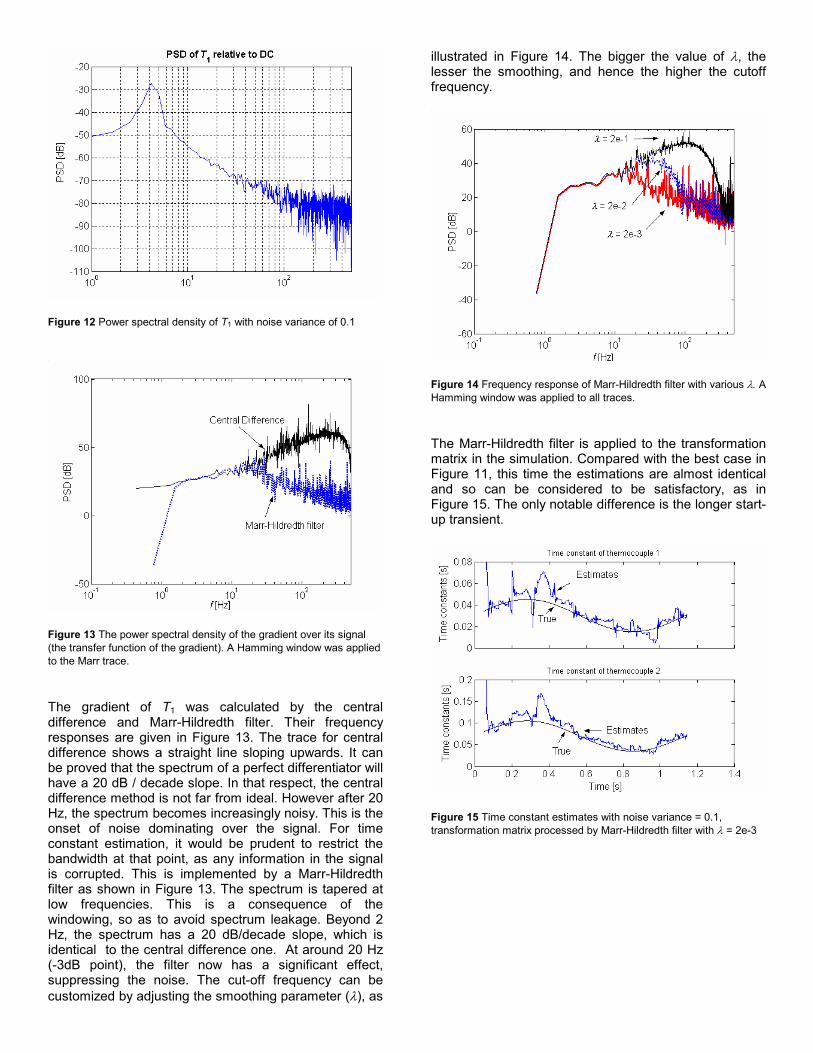
Figure 12 Power spectral density of T1 with noise variance of 0.1

Figure 13 The power spectral density of the gradient over its signal (the transfer function of the gradient). A Hamming window was applied to the Marr trace.

The gradient of T1 was calculated by the central difference and Marr-Hildredth filter. Their frequency responses are given in Figure 13. The trace for central difference shows a straight line sloping upwards. It can be proved that the spectrum of a perfect differentiator will have a 20 dB / decade slope. In that respect, the central difference method is not far from ideal. However after 20 Hz, the spectrum becomes increasingly noisy. This is the onset of noise dominating over the signal. For time constant estimation, it would be prudent to restrict the bandwidth at that point, as any information in the signal is corrupted. This is implemented by a Marr-Hildredth filter as shown in Figure 13. The spectrum is tapered at low frequencies. This is a consequence of the windowing, so as to avoid spectrum leakage. Beyond 2 Hz, the spectrum has a 20 dB/decade slope, which is identical to the central difference one. At around 20 Hz (-3dB point), the filter now has a significant effect, suppressing the noise. The cut-off frequency can be customized by adjusting the smoothing parameter (λ), as

illustrated in Figure 14. The bigger the value of λ, the lesser the smoothing, and hence the higher the cutoff frequency.

Figure 14 Frequency response of Marr-Hildredth filter with various λ. A Hamming window was applied to all traces.

The Marr-Hildredth filter is applied to the transformation matrix in the simulation. Compared with the best case in Figure 11, this time the estimations are almost identical and so can be considered to be satisfactory, as in Figure 15. The only notable difference is the longer start-up transient.

Figure 15 Time constant estimates with noise variance = 0.1, transformation matrix processed by Marr-Hildredth filter with λ = 2e-3

AIR RIG STUDY

The second phase of the model validation is to apply the Kalman filter to a well-controlled experiment. Simulation is often too simplistic, and may miss out important features from the real world. The object in the air rig study is to investigate the practicality of the technique.

Experiments were conducted with the air test rig at various temperature frequencies. The fundamental frequencies (fT) tested were from 2 Hz, up to 50 Hz. This is equivalent to a 4-stroke engine running from 240 to 6000 rpm. The shutter in the mixing valve was designed to minimize velocity variation. Measurements from the hot wire have shown the mean velocity at the outlet was nearly constant at 21 m/s for all fT. The turbulence intensities were also roughly constant at 6%. Since the temperature only fluctuated from 90 to 120°C and the flow velocity did not change significantly, the time constants should have small variations only. The Marr-Hildredth filter was applied in the same manner as in the simulation study. The time constant estimates in 5 temperature cycles are given in Figure 16. Both of them have unusual fluctuations. For example, τ2 can oscillate from 0.02 s to 0.06 s at the same frequency as the air temperature. These results do not seem to be plausible.

Figure 16 Time constant estimates at fT = 2.6 Hz. Subscript 2 and 3 denotes 0.002” and 0.003” thermocouples respectively.

Offset Errors and Normalization

Further investigation showed that the mean values of the thermocouples did not agree. There was about a 2.1 K difference. The mean values represent the DC component of the signals, and so should be unaffected by the thermal inertia of the thermocouples. It turned out that the amplifiers of each thermocouple had different offsets from ground, and hence the difference in the mean values. In measurement terms, 2 K difference is quite acceptable, but given that the raw temperature ranges measured by the thermocouples were only 25 – 30 K, this could seriously impair the temperature reconstruction. All two-thermocouple techniques rely on

the assumption that they sense the same temperature. If the measurement is offset by some external means, the assumption will break down, and the techniques will certainly fail. As a demonstration, the simulation can be re-run with offset intentionally added to one thermocouple signal. When this is done, the time constant estimates also show large swings between the true values at the temperature frequency; see Figure 17.

Figure 17 Adverse effect of offset errors demonstrated by a simulation

The thermocouple signals were therefore normalized to have a common mean value. The time constants were re-estimated as shown in Figure 18. Both time constants now have much smaller variations. Their high frequency components may indicate the turbulence in the flow.

Figure 18 Time constant estimates at fT = 2.6 Hz using the normalized signals.

With these time constant estimates, the thermocouple temperatures are reconstructed and plotted against the true gas temperature in Figure 19. Unlike the reconstructed temperature, the waveform of the true gas temperature is not well-defined. This could be the effect

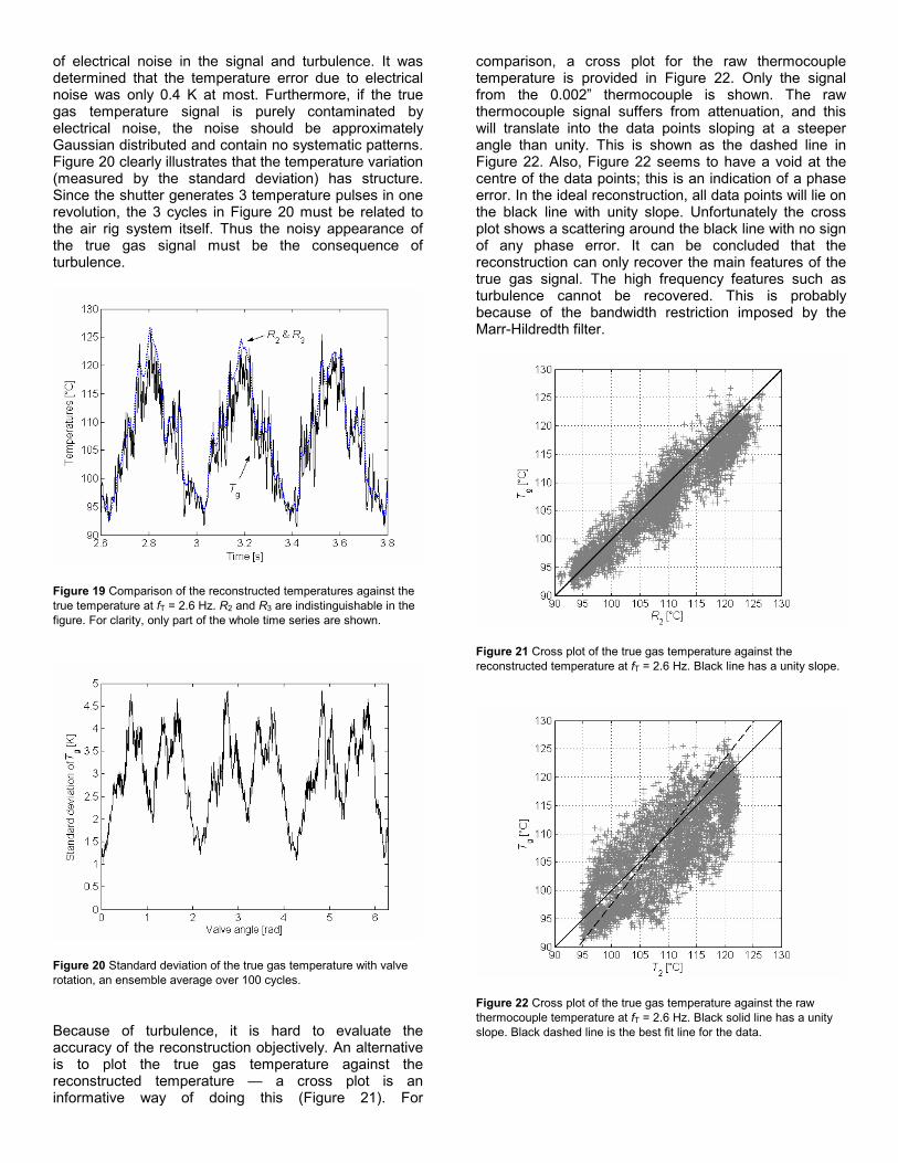
of electrical noise in the signal and turbulence. It was determined that the temperature error due to electrical noise was only 0.4 K at most. Furthermore, if the true gas temperature signal is purely contaminated by electrical noise, the noise should be approximately Gaussian distributed and contain no systematic patterns. Figure 20 clearly illustrates that the temperature variation (measured by the standard deviation) has structure. Since the shutter generates 3 temperature pulses in one revolution, the 3 cycles in Figure 20 must be related to the air rig system itself. Thus the noisy appearance of the true gas signal must be the consequence of turbulence.

Figure 19 Comparison of the reconstructed temperatures against the true temperature at fT = 2.6 Hz. R2 and R3 are indistinguishable in the figure. For clarity, only part of the whole time series are shown.

Figure 20 Standard deviation of the true gas temperature with valve rotation, an ensemble average over 100 cycles.

Because of turbulence, it is hard to evaluate the accuracy of the reconstruction objectively. An alternative is to plot the true gas temperature against the reconstructed temperature — a cross plot is an informative way of doing this (Figure 21). For

comparison, a cross plot for the raw thermocouple temperature is provided in Figure 22. Only the signal from the 0.002” thermocouple is shown. The raw thermocouple signal suffers from attenuation, and this will translate into the data points sloping at a steeper angle than unity. This is shown as the dashed line in Figure 22. Also, Figure 22 seems to have a void at the centre of the data points; this is an indication of a phase error. In the ideal reconstruction, all data points will lie on the black line with unity slope. Unfortunately the cross plot shows a scattering around the black line with no sign of any phase error. It can be concluded that the reconstruction can only recover the main features of the true gas signal. The high frequency features such as turbulence cannot be recovered. This is probably because of the bandwidth restriction imposed by the Marr-Hildredth filter.

Figure 21 Cross plot of the true gas temperature against the reconstructed temperature at fT = 2.6 Hz. Black line has a unity slope.

Figure 22 Cross plot of the true gas temperature against the raw thermocouple temperature at fT = 2.6 Hz. Black solid line has a unity slope. Black dashed line is the best fit line for the data.

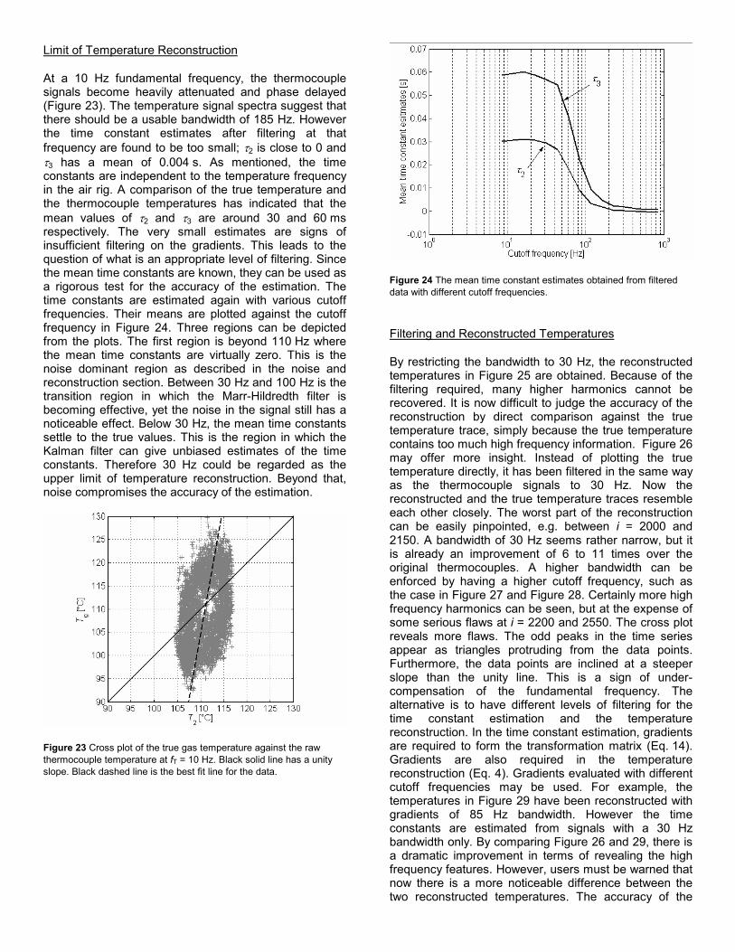
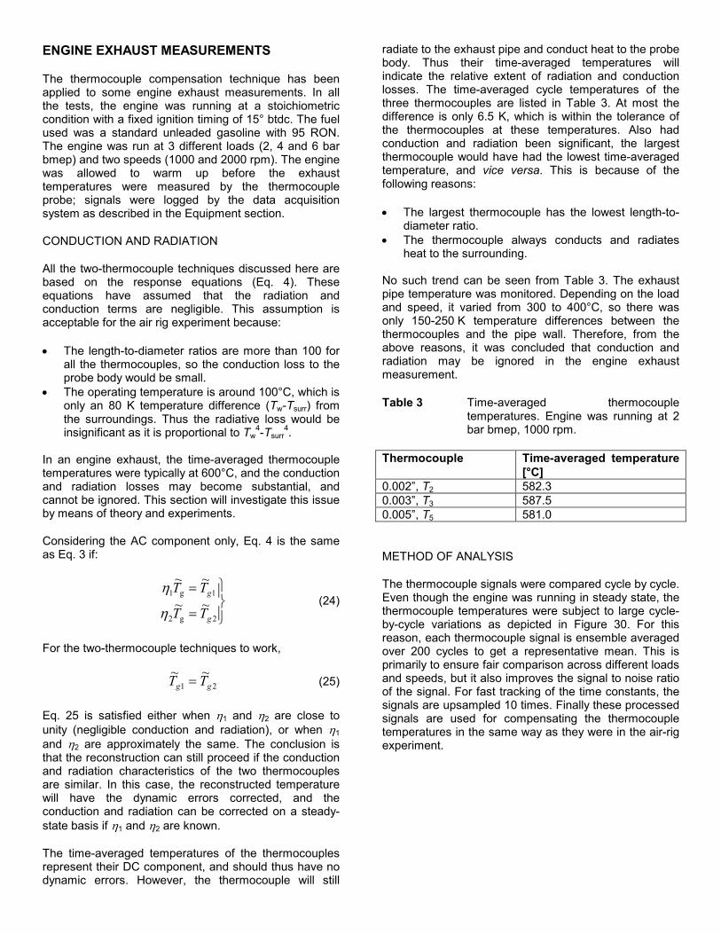
Limit of Temperature Reconstruction

At a 10 Hz fundamental frequency, the thermocouple signals become heavily attenuated and phase delayed (Figure 23). The temperature signal spectra suggest that there should be a usable bandwidth of 185 Hz. However the time constant estimates after filtering at that frequency are found to be too small; τ2 is close to 0 and τ3 has a mean of 0.004 s. As mentioned, the time constants are independent to the temperature frequency in the air rig. A comparison of the true temperature and the thermocouple temperatures has indicated that the mean values of τ2 and τ3 are around 30 and 60 ms respectively. The very small estimates are signs of insufficient filtering on the gradients. This leads to the question of what is an appropriate level of filtering. Since the mean time constants are known, they can be used as a rigorous test for the accuracy of the estimation. The time constants are estimated again with various cutoff frequencies. Their means are plotted against the cutoff frequency in Figure 24. Three regions can be depicted from the plots. The first region is beyond 110 Hz where the mean time constants are virtually zero. This is the noise dominant region as described in the noise and reconstruction section. Between 30 Hz and 100 Hz is the transition region in which the Marr-Hildredth filter is becoming effective, yet the noise in the signal still has a noticeable effect. Below 30 Hz, the mean time constants settle to the true values. This is the region in which the Kalman filter can give unbiased estimates of the time constants. Therefore 30 Hz could be regarded as the upper limit of temperature reconstruction. Beyond that, noise compromises the accuracy of the estimation.

Figure 23 Cross plot of the true gas temperature against the raw thermocouple temperature at fT = 10 Hz. Black solid line has a unity slope. Black dashed line is the best fit line for the data.

Figure 24 The mean time constant estimates obtained from filtered data with different cutoff frequencies.

Filtering and Reconstructed Temperatures

By restricting the bandwidth to 30 Hz, the reconstructed temperatures in Figure 25 are obtained. Because of the filtering required, many higher harmonics cannot be recovered. It is now difficult to judge the accuracy of the reconstruction by direct comparison against the true temperature trace, simply because the true temperature contains too much high frequency information. Figure 26 may offer more insight. Instead of plotting the true temperature directly, it has been filtered in the same way as the thermocouple signals to 30 Hz. Now the reconstructed and the true temperature traces resemble each other closely. The worst part of the reconstruction can be easily pinpointed, e.g. between i = 2000 and 2150. A bandwidth of 30 Hz seems rather narrow, but it is already an improvement of 6 to 11 times over the original thermocouples. A higher bandwidth can be enforced by having a higher cutoff frequency, such as the case in Figure 27 and Figure 28. Certainly more high frequency harmonics can be seen, but at the expense of some serious flaws at i = 2200 and 2550. The cross plot reveals more flaws. The odd peaks in the time series appear as triangles protruding from the data points. Furthermore, the data points are inclined at a steeper slope than the unity line. This is a sign of under-compensation of the fundamental frequency. The alternative is to have different levels of filtering for the time constant estimation and the temperature reconstruction. In the time constant estimation, gradients are required to form the transformation matrix (Eq. 14). Gradients are also required in the temperature reconstruction (Eq. 4). Gradients evaluated with different cutoff frequencies may be used. For example, the temperatures in Figure 29 have been reconstructed with gradients of 85 Hz bandwidth. However the time constants are estimated from signals with a 30 Hz bandwidth only. By comparing Figure 26 and 29, there is a dramatic improvement in terms of revealing the high frequency features. However, users must be warned that now there is a more noticeable difference between the two reconstructed temperatures. The accuracy of the

reconstruction has deteriorated. At the peaks, an error of 5 K is common. The root of the problems is that components at 85 Hz were not considered by the Kalman filter, and the reconstruction temperatures possess no maximum likelihood (evidence), so the accuracy can no longer be guaranteed. Therefore it is concluded that this method of bandwidth improvement is only suitable for a qualitative study, in which the absolute value of the temperature is unimportant.

Figure 25 Comparison of the reconstructed temperatures against the true temperature at fT = 10 Hz. R2 and R3 are indistinguishable in the figure. For clarity, only part of the whole time series is shown.

Figure 26 Comparison of the reconstructed temperatures against the true temperature at fT = 10 Hz. R2 and R3 are indistinguishable in the figure. All signals have their bandwidth restricted to 30 Hz.

Figure 27 Comparison of the reconstructed temperatures against the true temperature at fT = 10 Hz. All signals have their bandwidth restricted to 54 Hz.

Figure 28 Cross plot of the true gas temperature against the raw thermocouple temperature at fT = 10 Hz. All signals have their bandwidth restricted to 54 Hz.

Figure 29 Effect of different filtering, an 85 Hz cutoff is used for reconstruction, while a 30 Hz cutoff is used for time constant estimation.

ENGINE EXHAUST MEASUREMENTS

The thermocouple compensation technique has been applied to some engine exhaust measurements. In all the tests, the engine was running at a stoichiometric condition with a fixed ignition timing of 15° btdc. The fuel used was a standard unleaded gasoline with 95 RON. The engine was run at 3 different loads (2, 4 and 6 bar bmep) and two speeds (1000 and 2000 rpm). The engine was allowed to warm up before the exhaust temperatures were measured by the thermocouple probe; signals were logged by the data acquisition system as described in the Equipment section.

CONDUCTION AND RADIATION

All the two-thermocouple techniques discussed here are based on the response equations (Eq. 4). These equations have assumed that the radiation and conduction terms are negligible. This assumption is acceptable for the air rig experiment because:

• The length-to-diameter ratios are more than 100 for all the thermocouples, so the conduction loss to the probe body would be small.

• The operating temperature is around 100°C, which is only an 80 K temperature difference (Tw-Tsurr) from the surroundings. Thus the radiative loss would be insignificant as it is proportional to Tw

4-Tsurr4.

In an engine exhaust, the time-averaged thermocouple temperatures were typically at 600°C, and the conduction and radiation losses may become substantial, and cannot be ignored. This section will investigate this issue by means of theory and experiments.

Considering the AC component only, Eq. 4 is the same as Eq. 3 if:

=

=

2g2

1g1~~

~~

g

g

TT

TT

η

η (24)

For the two-thermocouple techniques to work,

21~~gg TT = (25)

Eq. 25 is satisfied either when η1 and η2 are close to unity (negligible conduction and radiation), or when η1 and η2 are approximately the same. The conclusion is that the reconstruction can still proceed if the conduction and radiation characteristics of the two thermocouples are similar. In this case, the reconstructed temperature will have the dynamic errors corrected, and the conduction and radiation can be corrected on a steady-state basis if η1 and η2 are known.

The time-averaged temperatures of the thermocouples represent their DC component, and should thus have no dynamic errors. However, the thermocouple will still

radiate to the exhaust pipe and conduct heat to the probe body. Thus their time-averaged temperatures will indicate the relative extent of radiation and conduction losses. The time-averaged cycle temperatures of the three thermocouples are listed in Table 3. At most the difference is only 6.5 K, which is within the tolerance of the thermocouples at these temperatures. Also had conduction and radiation been significant, the largest thermocouple would have had the lowest time-averaged temperature, and vice versa. This is because of the following reasons:

• The largest thermocouple has the lowest length-to-diameter ratio.

• The thermocouple always conducts and radiates heat to the surrounding.

No such trend can be seen from Table 3. The exhaust pipe temperature was monitored. Depending on the load and speed, it varied from 300 to 400°C, so there was only 150-250 K temperature differences between the thermocouples and the pipe wall. Therefore, from the above reasons, it was concluded that conduction and radiation may be ignored in the engine exhaust measurement.

Table 3 Time-averaged thermocouple temperatures. Engine was running at 2 bar bmep, 1000 rpm.

Thermocouple Time-averaged temperature [°C]

0.002”, T2 582.3 0.003”, T3 587.5 0.005”, T5 581.0

METHOD OF ANALYSIS

The thermocouple signals were compared cycle by cycle. Even though the engine was running in steady state, the thermocouple temperatures were subject to large cycle-by-cycle variations as depicted in Figure 30. For this reason, each thermocouple signal is ensemble averaged over 200 cycles to get a representative mean. This is primarily to ensure fair comparison across different loads and speeds, but it also improves the signal to noise ratio of the signal. For fast tracking of the time constants, the signals are upsampled 10 times. Finally these processed signals are used for compensating the thermocouple temperatures in the same way as they were in the air-rig experiment.

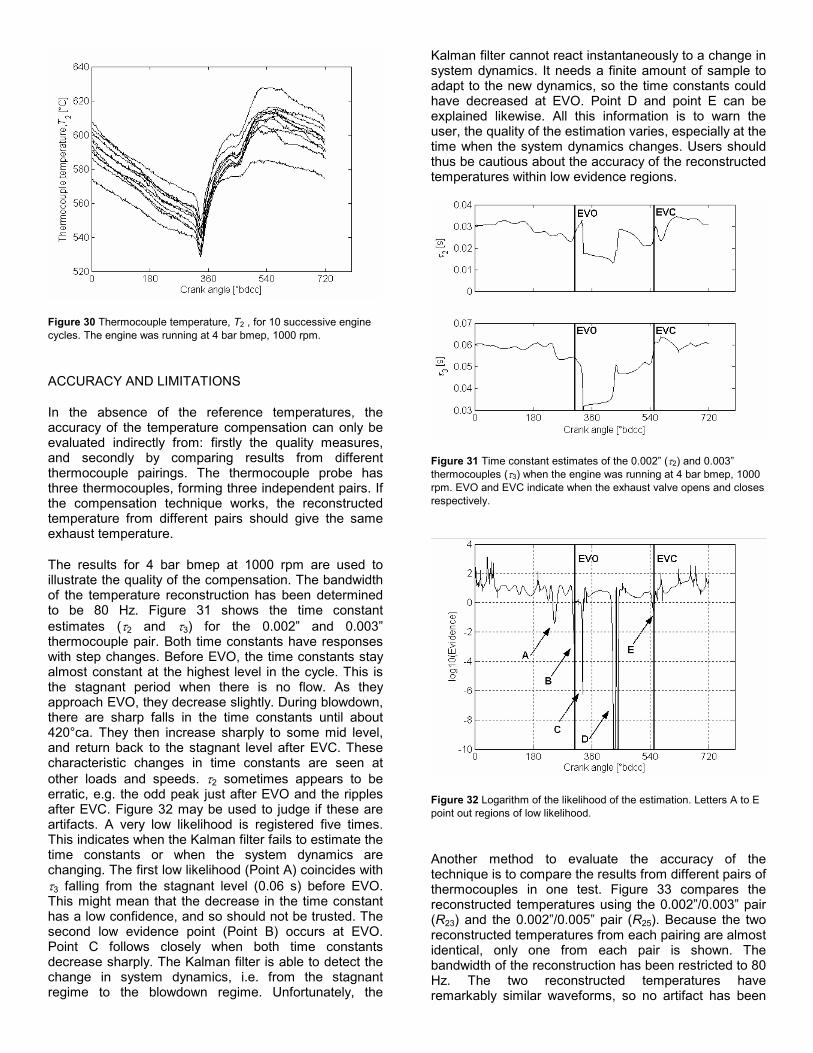
Figure 30 Thermocouple temperature, T2 , for 10 successive engine cycles. The engine was running at 4 bar bmep, 1000 rpm.

ACCURACY AND LIMITATIONS

In the absence of the reference temperatures, the accuracy of the temperature compensation can only be evaluated indirectly from: firstly the quality measures, and secondly by comparing results from different thermocouple pairings. The thermocouple probe has three thermocouples, forming three independent pairs. If the compensation technique works, the reconstructed temperature from different pairs should give the same exhaust temperature.

The results for 4 bar bmep at 1000 rpm are used to illustrate the quality of the compensation. The bandwidth of the temperature reconstruction has been determined to be 80 Hz. Figure 31 shows the time constant estimates (τ2 and τ3) for the 0.002” and 0.003” thermocouple pair. Both time constants have responses with step changes. Before EVO, the time constants stay almost constant at the highest level in the cycle. This is the stagnant period when there is no flow. As they approach EVO, they decrease slightly. During blowdown, there are sharp falls in the time constants until about 420°ca. They then increase sharply to some mid level, and return back to the stagnant level after EVC. These characteristic changes in time constants are seen at other loads and speeds. τ2 sometimes appears to be erratic, e.g. the odd peak just after EVO and the ripples after EVC. Figure 32 may be used to judge if these are artifacts. A very low likelihood is registered five times. This indicates when the Kalman filter fails to estimate the time constants or when the system dynamics are changing. The first low likelihood (Point A) coincides with τ3 falling from the stagnant level (0.06 s) before EVO. This might mean that the decrease in the time constant has a low confidence, and so should not be trusted. The second low evidence point (Point B) occurs at EVO. Point C follows closely when both time constants decrease sharply. The Kalman filter is able to detect the change in system dynamics, i.e. from the stagnant regime to the blowdown regime. Unfortunately, the

Kalman filter cannot react instantaneously to a change in system dynamics. It needs a finite amount of sample to adapt to the new dynamics, so the time constants could have decreased at EVO. Point D and point E can be explained likewise. All this information is to warn the user, the quality of the estimation varies, especially at the time when the system dynamics changes. Users should thus be cautious about the accuracy of the reconstructed temperatures within low evidence regions.

Figure 31 Time constant estimates of the 0.002” (τ2) and 0.003” thermocouples (τ3) when the engine was running at 4 bar bmep, 1000 rpm. EVO and EVC indicate when the exhaust valve opens and closes respectively.

Figure 32 Logarithm of the likelihood of the estimation. Letters A to E point out regions of low likelihood.

Another method to evaluate the accuracy of the technique is to compare the results from different pairs of thermocouples in one test. Figure 33 compares the reconstructed temperatures using the 0.002”/0.003” pair (R23) and the 0.002”/0.005” pair (R25). Because the two reconstructed temperatures from each pairing are almost identical, only one from each pair is shown. The bandwidth of the reconstruction has been restricted to 80 Hz. The two reconstructed temperatures have remarkably similar waveforms, so no artifact has been

introduced. Comparing their magnitude, the peak temperatures have a largest difference of 30 K. Apart from this, R23 and R25 typically differ by 10 K only, which is quite acceptable, given that the fluctuations in T2, T3 and T5 are so heavily attenuated. Moreover, the R23 and R25 traces are in phase, for example, both show an immediate cooling after EVO. In summary, the above findings have confirmed that the technique is robust, and suitable for applying to exhaust temperature measurements.

Figure 33 Comparison of the reconstructed temperatures (R23, R25) from different pairings. The uncompensated temperatures are also shown. The engine was running at 2 bar bmep, 1000 rpm.

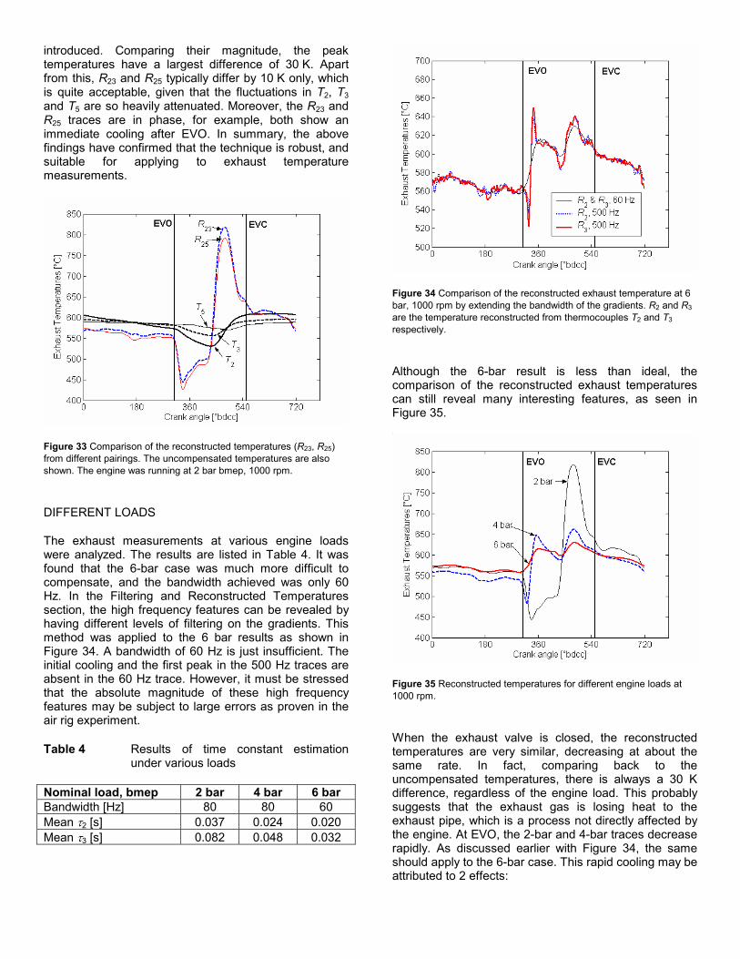
DIFFERENT LOADS

The exhaust measurements at various engine loads were analyzed. The results are listed in Table 4. It was found that the 6-bar case was much more difficult to compensate, and the bandwidth achieved was only 60 Hz. In the Filtering and Reconstructed Temperatures section, the high frequency features can be revealed by having different levels of filtering on the gradients. This method was applied to the 6 bar results as shown in Figure 34. A bandwidth of 60 Hz is just insufficient. The initial cooling and the first peak in the 500 Hz traces are absent in the 60 Hz trace. However, it must be stressed that the absolute magnitude of these high frequency features may be subject to large errors as proven in the air rig experiment.

Table 4 Results of time constant estimation under various loads

Nominal load, bmep 2 bar 4 bar 6 bar Bandwidth [Hz] 80 80 60 Mean τ2 [s] 0.037 0.024 0.020 Mean τ3 [s] 0.082 0.048 0.032

Figure 34 Comparison of the reconstructed exhaust temperature at 6 bar, 1000 rpm by extending the bandwidth of the gradients. R2 and R3 are the temperature reconstructed from thermocouples T2 and T3 respectively.

Although the 6-bar result is less than ideal, the comparison of the reconstructed exhaust temperatures can still reveal many interesting features, as seen in Figure 35.

Figure 35 Reconstructed temperatures for different engine loads at 1000 rpm.

When the exhaust valve is closed, the reconstructed temperatures are very similar, decreasing at about the same rate. In fact, comparing back to the uncompensated temperatures, there is always a 30 K difference, regardless of the engine load. This probably suggests that the exhaust gas is losing heat to the exhaust pipe, which is a process not directly affected by the engine. At EVO, the 2-bar and 4-bar traces decrease rapidly. As discussed earlier with Figure 34, the same should apply to the 6-bar case. This rapid cooling may be attributed to 2 effects:

1. Before EVO, the valve has been in contact with the seat for a while, so the valve surface in contact with the valve seat could be a few hundred Kelvin cooler than the gas at EVO. During the initial phase of the blowdown, the flow across the valve is a choked flow, which has very heat transfer coefficient. With the combination of a large temperature difference and a high heat transfer coefficient, the exhaust gas can lose a substantial amount of heat and hence the decrease in its temperature.

2. The measuring point is about 100 mm away from the exhaust port exit. There are some exhaust gases which left the cylinder at the end of the previous exhaust cycle and will have been stationary in the exhaust port while the valve has been closed. They have been cooled substantially because the cylinder head is maintained at about 100°C by the coolant. At the start of the blowdown, they are mixed with the hotter gas which has just left the cylinder [22]. Hence the exhaust temperature does not increase immediately after EVO.

For 4 bar and 6 bar bmep, what follows the rapid cooling is an increase in exhaust temperature to the first peak just before bdc. The gas temperatures decrease from this peak to a minimum at about 440°ca, then increase again until 480°ca. These general changes in exhaust temperatures agree with Caton & Heywood’s study [23], in which the exhaust temperature was measured by a resistance wire thermometer [7]. Heywood [22] pointed out that the local minimum at 440°ca is the transition from blowdown flow to displacement flow. Referring back to the time constant estimates in Figure 31, the time constants suddenly increase at this point, whilst the likelihood of the estimation in Figure 32 indicates there is a change in the system dynamics. The 2-bar result does not follow the trend. Perhaps the mass flux becomes so low at 2 bar bmep that it forms only a small proportion of the mixed gas (Reason 2), and so delays the temperature rise.

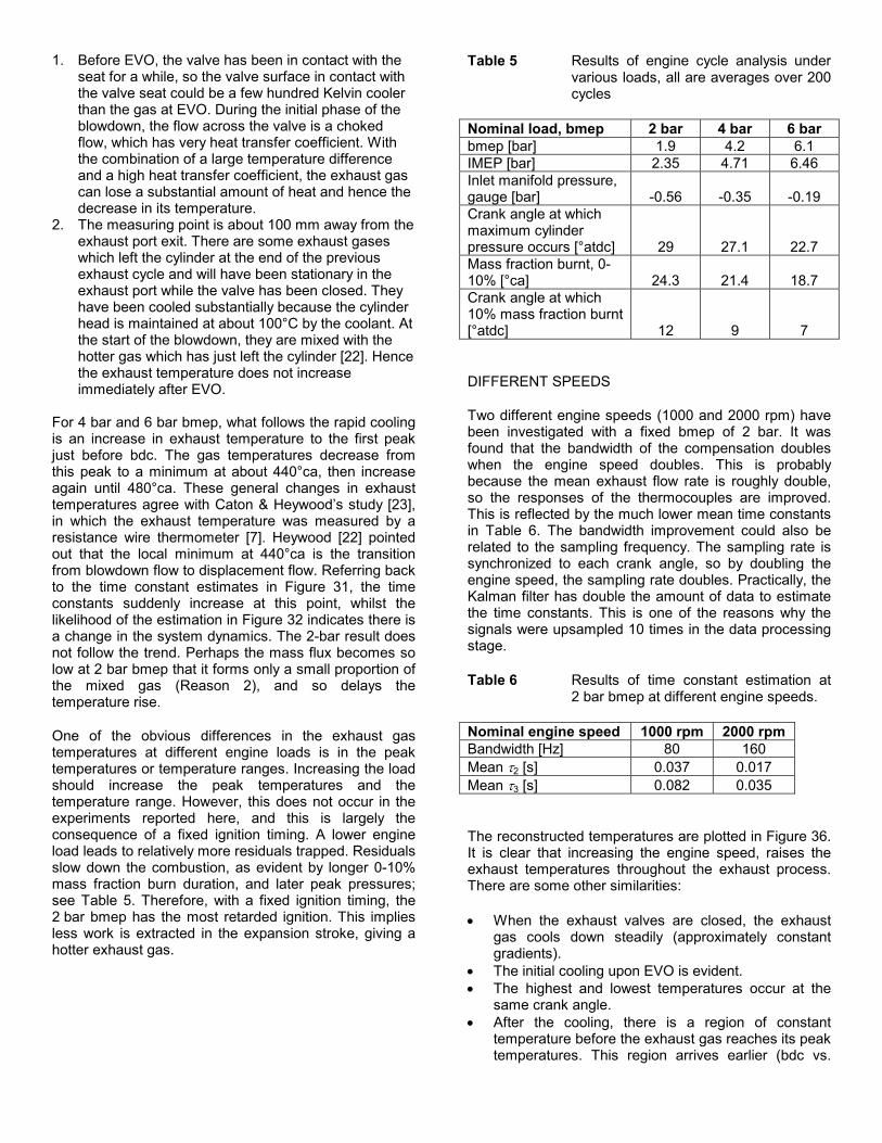
One of the obvious differences in the exhaust gas temperatures at different engine loads is in the peak temperatures or temperature ranges. Increasing the load should increase the peak temperatures and the temperature range. However, this does not occur in the experiments reported here, and this is largely the consequence of a fixed ignition timing. A lower engine load leads to relatively more residuals trapped. Residuals slow down the combustion, as evident by longer 0-10% mass fraction burn duration, and later peak pressures; see Table 5. Therefore, with a fixed ignition timing, the 2 bar bmep has the most retarded ignition. This implies less work is extracted in the expansion stroke, giving a hotter exhaust gas.

Table 5 Results of engine cycle analysis under various loads, all are averages over 200 cycles

Nominal load, bmep 2 bar 4 bar 6 bar bmep [bar] 1.9 4.2 6.1 IMEP [bar] 2.35 4.71 6.46 Inlet manifold pressure, gauge [bar] -0.56 -0.35 -0.19 Crank angle at which maximum cylinder pressure occurs [°atdc] 29 27.1 22.7 Mass fraction burnt, 0-10% [°ca] 24.3 21.4 18.7 Crank angle at which 10% mass fraction burnt [°atdc] 12 9 7

DIFFERENT SPEEDS

Two different engine speeds (1000 and 2000 rpm) have been investigated with a fixed bmep of 2 bar. It was found that the bandwidth of the compensation doubles when the engine speed doubles. This is probably because the mean exhaust flow rate is roughly double, so the responses of the thermocouples are improved. This is reflected by the much lower mean time constants in Table 6. The bandwidth improvement could also be related to the sampling frequency. The sampling rate is synchronized to each crank angle, so by doubling the engine speed, the sampling rate doubles. Practically, the Kalman filter has double the amount of data to estimate the time constants. This is one of the reasons why the signals were upsampled 10 times in the data processing stage.

Table 6 Results of time constant estimation at 2 bar bmep at different engine speeds.

Nominal engine speed 1000 rpm 2000 rpm Bandwidth [Hz] 80 160 Mean τ2 [s] 0.037 0.017 Mean τ3 [s] 0.082 0.035

The reconstructed temperatures are plotted in Figure 36. It is clear that increasing the engine speed, raises the exhaust temperatures throughout the exhaust process. There are some other similarities:

• When the exhaust valves are closed, the exhaust gas cools down steadily (approximately constant gradients).

• The initial cooling upon EVO is evident. • The highest and lowest temperatures occur at the

same crank angle. • After the cooling, there is a region of constant

temperature before the exhaust gas reaches its peak temperatures. This region arrives earlier (bdc vs.

30°abdc) and lasts longer (48 °ca vs. 33 °ca) at the higher speed.

This is still yet to be explained. What is required is to perform a 1-D unsteady flow simulation, so that measurements and a model can be compared directly. This should give some new insights into the underlying physics that governs the exhaust process.

Figure 36 Comparison of the reconstructed temperature at 2 bar bmep, different engine speeds.

CONCLUSIONS

The dynamic response of a thermocouple can be described by a time constant. Because it is too difficult to predict analytically, a thermocouple compensation technique has been developed to estimate the time constant in situ. By this means, the instantaneous gas temperature may be found, once the time constant is known. This technique is one of many 2-thermocouple techniques, which are based on the assumption that two thermocouples are exposed to the same temperature and velocity fields. It is based on a Kalman filter, and has the following advantages over other methods:

• No a priori assumptions for the time constant ratio • The data is analyzed recursively and the time

constants are estimated at each time step. There is no issue of window size.

• The two reconstructed temperatures may differ. This flexibility makes it less susceptible to noise.

• Qualitative measures of the estimation are provided to the user.

The Kalman filter has been commissioned in a simulation study and an air rig experiment. The simulation has shown that the Kalman filter performs well in virtually noiseless conditions, but returns unphysical estimates when a realistic level of noise is present. Noise will get amplified in the process of reconstruction, giving erroneous results. For successful estimation, the bandwidth of the signals has to be restricted by a filter.

This suppresses the high frequency noise, and the time derivatives can be found easily.

In the air rig experiment, with the aid of a reference thermometer, several practical issues were highlighted. First, offset errors exist between thermocouple signals, and this leads to the time constant estimates showing large departures from their true values. To solve this, the thermocouple signals have to be normalized. Second, with the bandwidth restriction (because of noise), the temperature reconstruction can only recover the main features of the true gas signal. The high frequency features such as turbulence cannot be recovered. The frequency limit of the temperature reconstruction has been established by looking at the mean time constant estimates at various cut-off frequencies. The unbiased estimates can be obtained when the mean values settle below a certain frequency. This sets the possible bandwidth improvement. Further improvement can be partially achieved by having different filtering levels for the time constant estimation and the temperature reconstruction, but it is only suitable for a qualitative study, since the accuracy is no longer guaranteed.

Finally, the technique has been applied to some engine exhaust measurements. By comparing the time-averaged temperature of the three thermocouples, it has been concluded that the relative extent of radiation and conduction losses are negligible. The likelihood of the estimation shows that the Kalman filter is able to detect the changes in system dynamics, e.g. from the stagnant regime to the blowdown regime. However, the Kalman filter needs a finite amount of sample to adapt to the new dynamics, hence the results of the transitional period should be used cautiously. The accuracy of the reconstruction is further examined by comparing the results from different pairs of thermocouples in one test. They are remarkably similar with the largest difference of 30 K at the peak temperatures which occur with high temperature gradients.

After reconstruction, the exhaust gas temperatures at all engine loads investigated, are seen to cool down at EVO. This is due to the large heat loss to the valve, and the mixing of the cooled gas in the exhaust pipe. At 4 bar and 6 bar bmep, the gas temperatures decreases from the first peak to a minimum and then increase again. These general changes agree with previous studies, which had a lower bandwidth [23]. It is found that increasing the engine load reduces the peak temperatures and the temperature ranges. This is due to a fixed ignition timing, resulting in retarded ignition for the lower engine loads. A higher engine speed raises the exhaust temperature throughout the exhaust process. The initial cooling upon EVO still exists. A region of constant temperature exists following the initial cooling. This remains unexplained. A 1-D unsteady flow simulation may give some insight into these exhaust processes.

ACKNOWLEDGMENTS

This work was supported by the Ford Motor Company. The first author (KK) would also like to acknowledge the financial support of Foundation for Research, Science and Technology of New Zealand.

REFERENCES

1. Koehlen, C., Holder, E., and Vent, G., Investigation of Post Oxidation and Its Dependency on Engine Combustion and Exhaust Manifold Design. SAE Paper 2002-01-0744, 2002.

2. Kee, R., O'Reilly, P.G., Fleck, R., and McEntee, P.T., Measurement of Exhaust Gas Temperatures in a High Performance Two-Stroke Engine. SAE Paper 983072, 1998.

3. Bauer, W., Tam, C., Heywood, J.B., and Ziegler, C., Fast Gas Temperature Measurement by Velocity of Sound for IC Engine Applications. SAE Paper 972826, 1997.

4. Andresen, P., Meijer, G., Schlüter, H., Voges, A., and Hentschel, W., Fluorescence Imaging Inside an Internal Combustion Engine using Tunable Excimer Lasers. Appl. Opt., 1990. 29: p. 2392-404.

5. Koch, A., Voges, H., Andresen, P., Schlüter, H., Wolff, D., Hentschel, W., Oppermann, W., and Rother, E., Planar Imaging of a Laboratory Flame and of Internal Combustion using UV Rayleigh and Fluorence Light. Appl. Phys. B, 1993. 56: p. 177-84.

6. Benson, R.S. and Brundrett, G.W., Development of a resistance wire thermometer for measuring transient temperatures in exhaust systems of internal combustion engines, in Temperature - Its Measurement and Control in Science and Industry. 1962, Reinhold: New York. p. 631-653.

7. Benson, R.S., Measurement of transient exhaust temperatures in I.C. engines. The Engineer, 1964. 217: p. 376-383.

8. Scadron, M.D. and Warshawsky, I., Experimental Determination of Time Constants and Nusselt Numbers for Bare-Wire Thermocouples in High-Velocity Air Streams and Analytic Approximation of Conduction and Radiation Errors. NACA TN 2599, 1952. p. 5-6, 20-22, 40-45.

9. Cambray, P., Measuring Thermocouple Time Constants: A New Method. Combustion Science and Technology, 1986. 45: p. 221-224.

10. Forney, L.J. and Fralick, G.C., Two wire thermocouple: Frequency response in constant flow. Review of Scientific Instruments, 1994. 65(10): p. 3252-3256.

11. O'Reilly, P.G., Kee, R.J., Fleck, R., and McEntee, P.T., Two-wire thermocouples: A nonlinear state estimation approach to temperature reconstruction. Review of Scientific Instruments, 2001. 72(8): p. 3449-3457.

12. Tagawa, M. and Ohta, Y., Two-Thermocouple Probe for Fluctuating Temperature Measurement in Combustion- Rational Estimation of Mean and

Fluctuating Time Constants. Combustion and Flame, 1997. 109: p. 540-560.

13. Tagawa, M., Shimoji, T., and Ohta, Y., A two-thermocouple probe technique for estimating thermocouple time constants in flows with combustion: In situ parameter identification of a first-order lag system. Review of Scientific Instruments, 1998. 69(9): p. 3370-3378.

14. Tagawa, M., Kato, K., and Ohta, Y., Response compensation of temperature sensors: Frequency-domain estimation of thermal time constants. Review of Scientific Instruments, 2003. 74(6): p. 3171-3174.

15. Hung, P.C.F., McLoone, S., Irwin, G., and Kee, R.J. A Total Least Squares Approach to Sensor Characterisation. 13th IFAC Symposium on System Identification, SYSID-2003, Rotterdam, The Netherlands, August 27-29, 2003.

16. Kar, K., Three-Thermocouple Technique for Fluctuating Temperature Measurement. Internal Report, Department of Engineering Science, University of Oxford, 2002. p. 3-15.

17. Penny, W.D. and Roberts, S., Dynamic Linear Models, Recursive Least Squares and Steepest-Descent Learning. Technical Report, Department of Electrical and Electronic Engineering, Imperial College of Science and Technology and Medicine, 1998. p. 1-3.

18. Jazwinski, A.H., Adaptive filtering. Automatica, 1969. 5: p. 475-485.

19. Bruun, H.H., Hot-Wire Anemometry. 1995, Oxford: Oxford University Press.

20. Stone, C.R., Introduction to Internal Combustion Engines. Third ed. 1999, Basingstoke: Macmillan Press Ltd.

21. Oude Nijeweme, D.J., Kok, J.B.W., Stone, C.R., and Wyszynski, L., Unsteady in-cylinder heat transfer in a spark ignition engine: experiments and modelling. Proceeding Institution of Mechanical Engineers, 2001. 215(D): p. 747-760.

22. Heywood, J.B., Internal Combustion Engine Fundamentals. 1988, New York: McGraw-Hill Book Company.

23. Caton, J.A. and Heywood, J.B., An Experimental and Analytical Study of Heat Transfer in an Engine Exhaust Port. Int. J. Heat Mass Transfer, 1981. 24(4): p. 581-595.

CONTACT

Any comments and questions should be directed to Kenneth Kar (kenneth.kar@eng.ox.ac.uk) or Richard Stone (richard.stone@eng.ox.ac.uk). The corresponding address is: Department of Engineering Science, University of Oxford, Parks Road, Oxford OX1 3PJ

DEFINITIONS, ACRONYMS, ABBREVIATIONS

AC Alternating current, the fluctuating component of a signal

bdcc Bottom dead centre at the start of the compression stroke

bmep Brake mean effective pressure, bar

btdc Before top dead centre

DC Direct current, zero frequency

EGT Exhaust gas temperature

EVC Exhaust Valve Closure

EVO Exhaust Valve Opening

FTP-75 Federal Test Procedure

imep Indicated mean effective pressure, bar

PSD Power spectral density

c Specific heat, kJ/kgK

d Diameter of thermocouple junction, m

e Noise; prediction error

F Transformation matrix

f Frequency, Hz

G Flow matrix

g(t) Gaussian kernel

h Heat transfer coefficient, W/m2K

h(x) Ramp function

i ith sample of the digitized data

I Identity matrix

k Thermal conductivity, W/mK

K Kalman gain matrix

m Coefficient of Reynolds number in the Nusselt correlation

R Covariance of the latent variables prior the observation

R Reconstructed temperature, °C

T Temperature, K/ °C

t Time, s

v Observation noise

V Observation noise covariance matrix

w Static noise

W State noise covariance matrix

x Coordinate system in the axial direction of the thermocouple wire

y Multivariate observations

α Time constant ratio

ε Emissivity

η Radiation and conduction correction factor

λ Smoothing parameter of the Marr-Hildredth filter

θ Latent variable vector

ρ Density, kg/m3

Σ Covariance of the latent variables

σ Stefan-Boltzmann constant; variance

τ Time constant, s

ξ Mean squared difference between two reconstructed temperatures, K2

Superscript

— (overbar) Discrete Fourier transform

^ Estimated value

~ Fluctuation about the mean value

T Transpose of a matrix

Subscript

1 Thermocouple 1

2 Thermocouple 2; Thermocouple with a nominal diameter of 0.002”

23 0.002” and 0.003” thermocouple pair

25 0.002” and 0.005” thermocouple pair

3 Thermocouple with a nominal diameter of 0.003”

5 Thermocouple with a nominal diameter of 0.005”

den Denominator

g Gas

num Numerator

q0 No state noise condition

surr Surroundings

T Temperature

w Wire

y Prediction

θ Latent variables