Instance-Based Learning

0.

The k-NN algorithm: simple applicationCMU, 2006 fall, final exam, pr. 2

Consider the training setin the 2-dimensional Eu-clidean space shown inthe nearby table.

a. Represent the trainingdata in the 2D space.

b. What are the pre-dictions of the 3- 5- and7-nearest-neighbor classi-fiers at the point (1,1)?

x y−1 1 −0 1 +0 2 −1 −1 −1 0 +1 2 +2 2 −2 3 +

Solution:

b. k = 3: +; k = 5: +; k = 7: −.

y

−1 0 1 2 3

−1

1

2

3

x

1.

Drawing decision boundaries and decision surfaces

for the 1-NN classifier

Voronoi Diagrams

CMU, 2010 spring, E. Xing, T. Mitchell, A. Singh,

HW1, pr. 3.1

2.

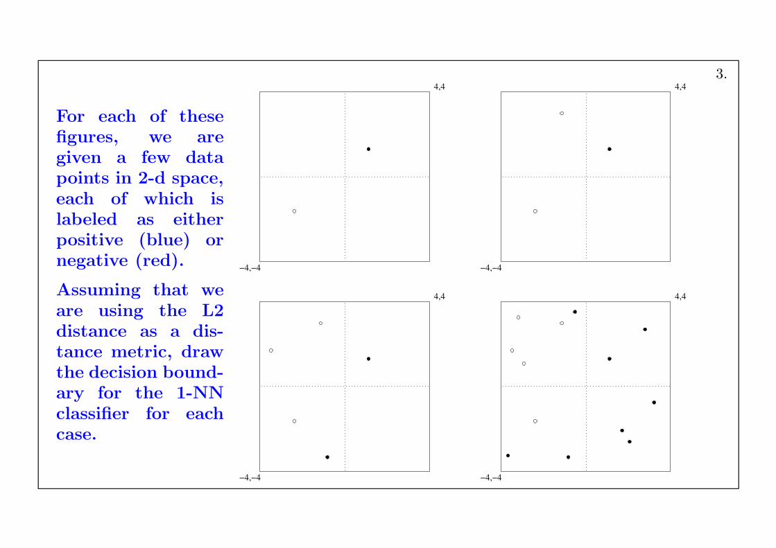
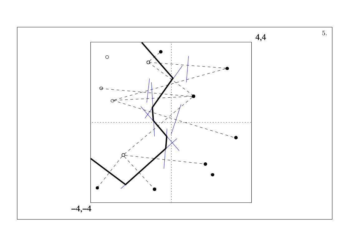
For each of thesefigures, we aregiven a few datapoints in 2-d space,each of which islabeled as eitherpositive (blue) ornegative (red).

Assuming that weare using the L2distance as a dis-tance metric, drawthe decision bound-ary for the 1-NNclassifier for eachcase.

−4,−4

4,4

−4,−4

4,4

−4,−4

4,4

−4,−4

4,4

3.

Solution

−4,−4

4,4

−4,−4

4,4

−4,−4

4,4

−4,−4

4,4

4.

−4,−4−4,−4

4,4

−4,−4

4,44,45.

Drawing decision boundaries and decision surfaces

for the 1-NN classifier

Voronoi Diagrams: DO IT YOURSELF

CMU, 2010 fall, Ziv Bar-Joseph, HW1, pr. 3.1

6.

For each of thenearby figures, youare given negative(◦) and positive (+)data points in the2D space.

Remember that a 1-NN classifier classi-fies a point accord-ing to the class of itsnearest neighbour.

Please draw theVoronoi diagramfor a 1-NN classifierusing Euclideandistance as thedistance metric foreach case.

−1

−1

0

0

1

1

2

2

−2−2

1.5

−1.5

0.5

−0.5

−1.5 1.50.5−0.5 −1

−1

0

0

1

1

2

2

−2−2

1.5

−1.5

0.5

−0.5

−1.5 1.50.5−0.5

−1

−1

0

0

1

1

2

2

−2−2

1.5

−1.5

0.5

−0.5

−1.5 1.50.5−0.5 −1

−1

0

0

1

1

2

2

−2

1.5

−1.5

0.5

−0.5

−1.5 1.50.5−0.5−2

7.

−1

−1

0

0

1

1

2

2

−2

1.5

−1.5

0.5

−0.5

−1.5 1.50.5−0.5−2

8.

Decision boundaries and decision surfaces:Comparison between the 1-NN and ID3 classifiers

CMU, 2007 fall, Carlos Guestrin, HW2, pr. 1.4

9.

For the data in the figure(s) below, sketch the decision surfaces obtained byapplyinga. the K-Nearest Neighbors algorithm with K = 1;b. the ID3 algorithm augmented with [the capacity to process] continousattributes.

0

0

1

1 2 3

3

2

4

4 5

5

6

6

x

y

0

0

1

1 2 3

3

2

4

4 5

5

6

6

x

y

10.

Solution: 1-NN

0

0

1

1

3

2

4

4 5

5

6

6

y

x2 3

0

0

1

1

3

2

4

4 5

5

6

6

y

x2 3

11.

Solution: ID3

01

53

2

4

1 20 3 4 5 6

2

3

4

5

6

0

1

y

x 1 20 3 4 5 6

2

3

4

5

6

0

1

y

x

12.

Instance-Based Learning

Some important properties

13.

k-NN and the Curse of Dimensionality

Proving that the number of examples needed by k-NN

grows exponentially with the number of features

CMU, 2010 fall, Aarti Singh, HW2, pr. 2.2

[Slides originally drawn by Diana Mı̂nzat, MSc student, FII, 2015 spring]

14.

Consider a set of n points x1, x2, ..., xn independently and uniformlydrawn from a p-dimensional zero-centered unit ball

B = {x : ‖x‖2 ≤ 1} ⊂ Rp,

where ‖x‖ =√x· x and · is the inner product in R

p.

In this problem we will study the size of the 1-nearest neigh-bourhood of the origin O and how it changes in relation to thedimension p, thereby gain intuition about the downside of k-NNin a high dimension space.

Formally, this size will be described as the distance from O to itsnearest neighbour in the set {x1, ..., xn}, denoted by d∗:

d∗ := min1≤i≤n

||xi ||,

which is a random variable since the sample is random.

15.

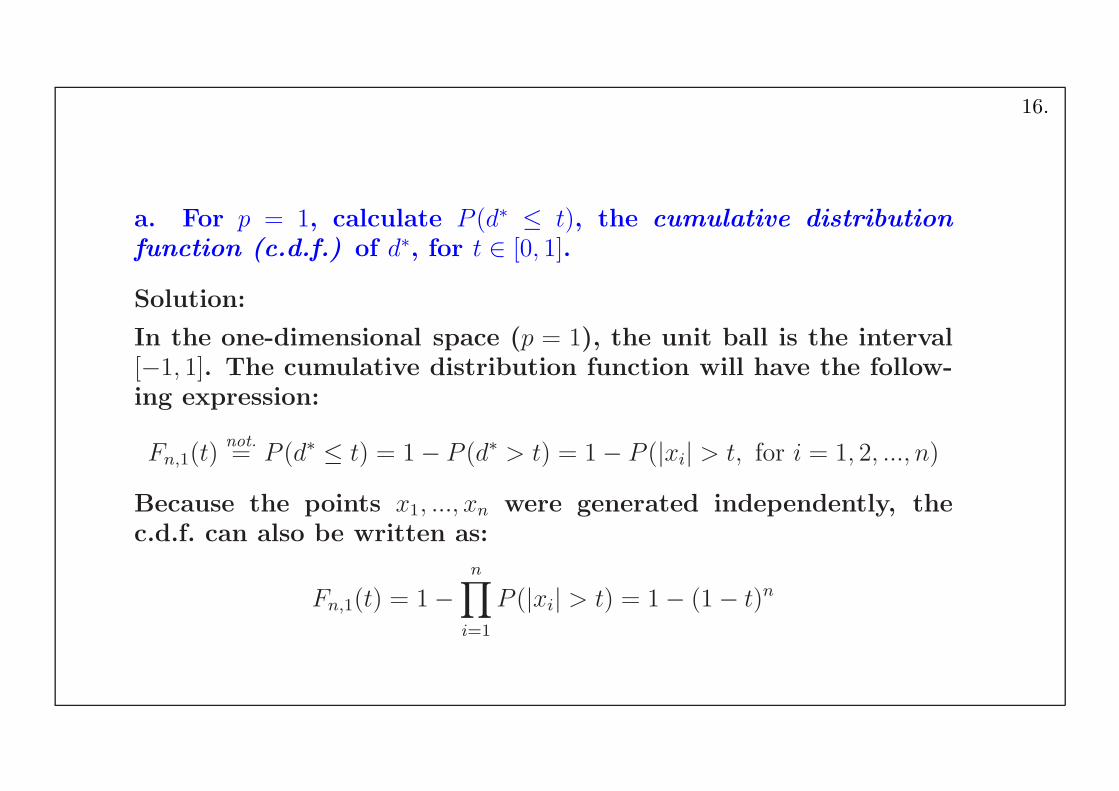
a. For p = 1, calculate P (d∗ ≤ t), the cumulative distributionfunction (c.d.f.) of d∗, for t ∈ [0, 1].

Solution:

In the one-dimensional space (p = 1), the unit ball is the interval[−1, 1]. The cumulative distribution function will have the follow-ing expression:

Fn,1(t)not.= P (d∗ ≤ t) = 1− P (d∗ > t) = 1− P (|xi| > t, for i = 1, 2, ..., n)

Because the points x1, ..., xn were generated independently, thec.d.f. can also be written as:

Fn,1(t) = 1−n∏

i=1

P (|xi| > t) = 1− (1− t)n

16.

b. Find the formula of the cumulative distribution function of d∗

for the general case, when p ∈ {1, 2, 3, ...}.

Hint: You may find the following fact useful: the volume of ap-dimensional ball with radius r is

Vp(r) =(r√π)

p

Γ(p

2+ 1

) ,

where Γ is Euler’s Gamma function, defined by

Γ

(

1

2

)

=√π, Γ(1) = 1, and Γ(x+ 1) = xΓ(x) for any x > 0.

Note: It can be easily shown that Γ(n + 1) = n! for all n ∈ N∗,

therefore the Gamma function is a generalization of the factorialfunction.

17.

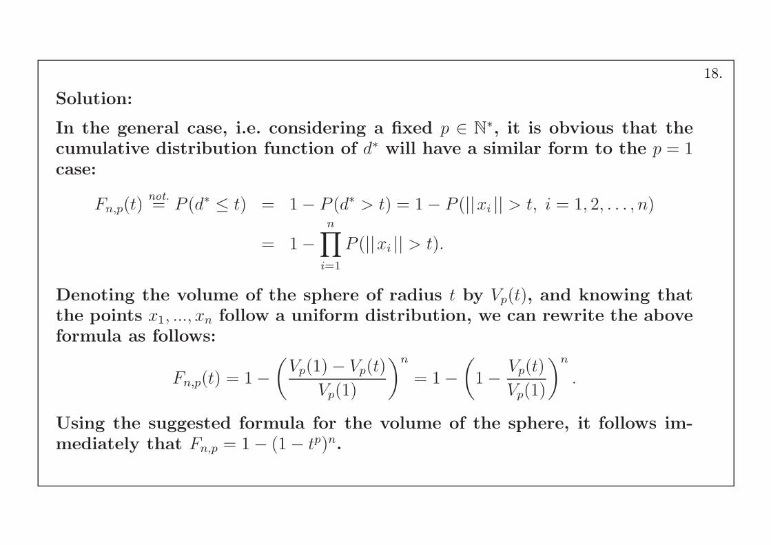
Solution:

In the general case, i.e. considering a fixed p ∈ N∗, it is obvious that the

cumulative distribution function of d∗ will have a similar form to the p = 1case:

Fn,p(t)not.= P (d∗ ≤ t) = 1− P (d∗ > t) = 1− P (||xi || > t, i = 1, 2, . . . , n)

= 1−n∏

i=1

P (||xi || > t).

Denoting the volume of the sphere of radius t by Vp(t), and knowing thatthe points x1, ..., xn follow a uniform distribution, we can rewrite the aboveformula as follows:

Fn,p(t) = 1−(

Vp(1)− Vp(t)

Vp(1)

)n

= 1−(

1− Vp(t)

Vp(1)

)n

.

Using the suggested formula for the volume of the sphere, it follows im-mediately that Fn,p = 1− (1− tp)n.

18.

c. What is the median of the random variable d∗ (i.e., the valueof t for which P (d∗ ≤ t) = 1/2) ? The answer should be a functionof both the sample size n and the dimension p.

Fix n = 100 and plot the values of the median function for p =1, 2, 3, ..., 100 with the median values on the y-axis and the valuesof p on the x-axis. What do you see?

Solution:

In order to find the median value of the random variable d∗, wewill solve the equation P (d∗ ≤ t) = 1/2 of variable t:

P (d∗ ≤ t) =1

2⇔ Fn,p(t) =

1

2b⇔ 1− (1− tp)n =

1

2⇔ (1− tp)n =

1

2

⇔ 1− tp =1

21/n⇔ tp = 1− 1

21/n

Therefore,

tmed(n, p) =

(

1− 1

21/n

)1/p

.

19.

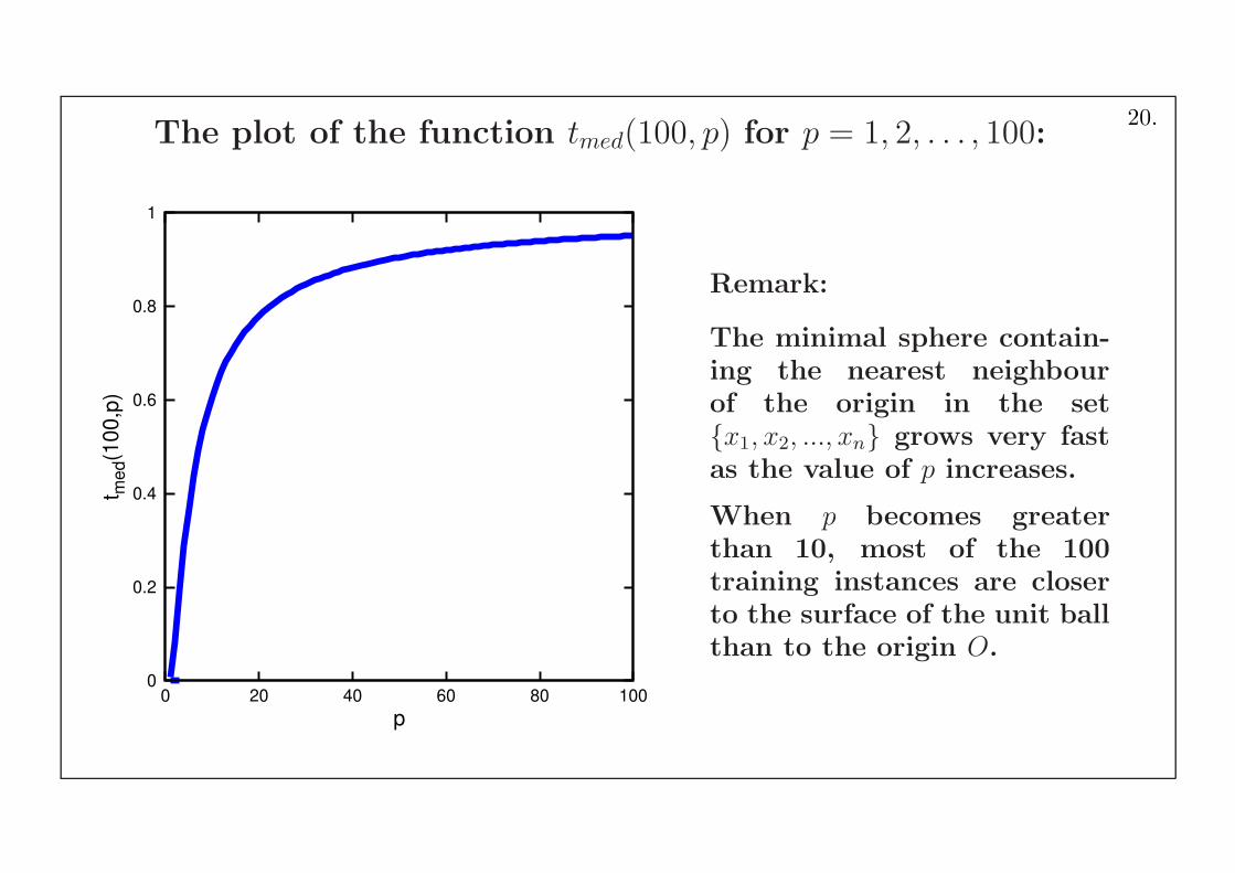
The plot of the function tmed(100, p) for p = 1, 2, . . . , 100:

0

0.2

0.4

0.6

0.8

1

0 20 40 60 80 100

t med(1

00

,p)

p

Remark:

The minimal sphere contain-ing the nearest neighbourof the origin in the set{x1, x2, ..., xn} grows very fastas the value of p increases.

When p becomes greaterthan 10, most of the 100training instances are closerto the surface of the unit ballthan to the origin O.

20.

d. Use the c.d.f. derived at point b to determine how large shouldthe sample size n be such that with probability at least 0.9, thedistance d∗ from O to its nearest neighbour is less than 1/2, i.e.,half way from O to the boundary of the ball.

The answer should be a function of p.Plot this function for p = 1, 2, . . . , 20 with the function values onthe y-axis and values of p on the x-axis. What do you see?

Hint : You may find useful the Taylor series expansion of ln(1−x):

ln(1− x) = −∞∑

i=1

xi

ifor − 1 ≤ x < 1.

21.

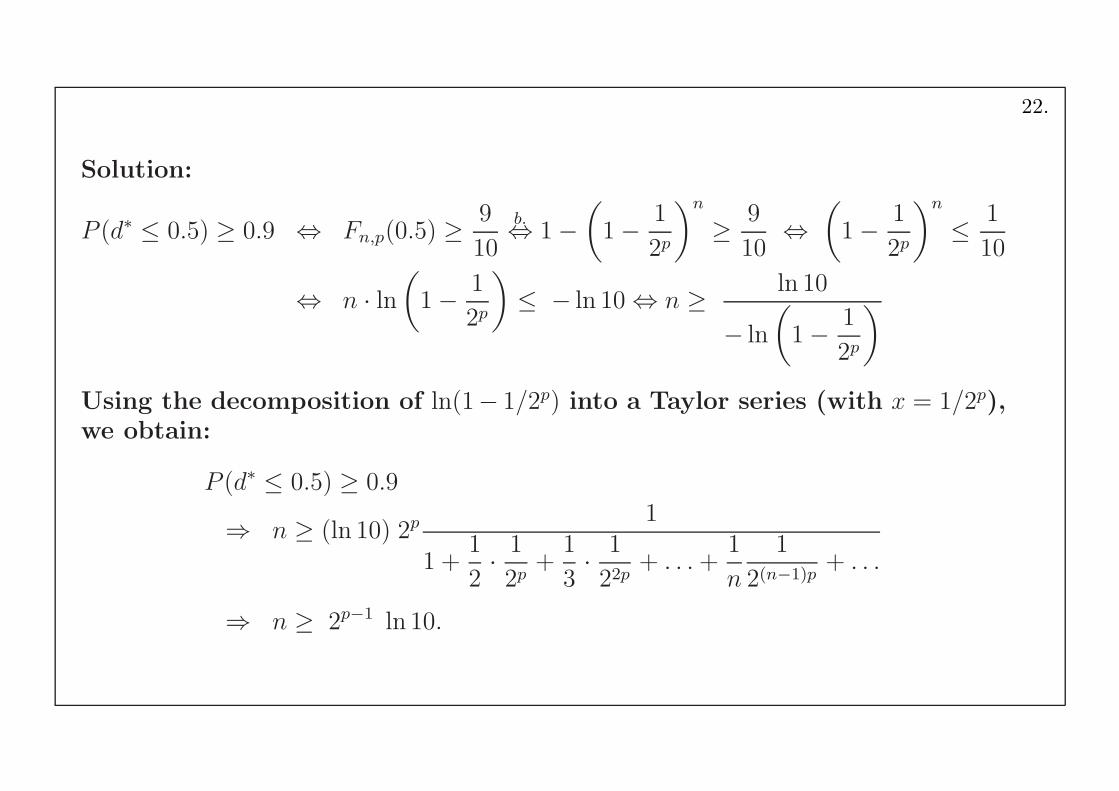
Solution:

P (d∗ ≤ 0.5) ≥ 0.9 ⇔ Fn,p(0.5) ≥9

10

b.⇔ 1−(

1− 1

2p

)n

≥ 9

10⇔

(

1− 1

2p

)n

≤ 1

10

⇔ n · ln(

1− 1

2p

)

≤ − ln 10 ⇔ n ≥ ln 10

− ln

(

1− 1

2p

)

Using the decomposition of ln(1− 1/2p) into a Taylor series (with x = 1/2p),we obtain:

P (d∗ ≤ 0.5) ≥ 0.9

⇒ n ≥ (ln 10) 2p1

1 +1

2· 1

2p+

1

3· 1

22p+ . . .+

1

n

1

2(n−1)p+ . . .

⇒ n ≥ 2p−1 ln 10.

22.

Note:

In order to obtain the last inequality in the above calculations, weconsidered the following two facts:

i.1

3 · 2p <1

4holds for any p ≥ 1, and

ii.1

n · 2(n−1)p≤ 1

2n⇔ 2n ≤ n · 2(n−1)p holds for any p ≥ 1 and n ≥ 2.

(This can be proven by induction on p).

So, we got:

1 +1

2· 1

2p+

1

3· 1

22p+ . . .+

1

n

1

2(n−1)p+ . . . <

1 +1

2+

1

4+ . . .+

1

2n+ . . . → 1

1− 1

2

= 2.

23.

The proven result

P (d∗ ≤ 0.5) ≥ 0.9 ⇒ n ≥ 2p−1 ln 10

means that the sample size neededfor the probability that d∗ < 0.5 islarge enough (9/10) grows expo-nentially with p.

0

0.5

1

1.5

2

2.5

0 5 10 15 20

-(ln

10

/ ln(

1-2-p

)) /

106

p

24.

e. Having solved the previous problems, what will you say aboutthe downside of k-NN in terms of n and p?

Solution:

The k-NN classifier works well when a test instance has a “dense”neighbourhood in the training data.

However, the analysis here suggests that in order to provide adense neighbourhood, the size of the training sample should beexponential in the dimension p, which is clearly infeasible for alarge p.

(Remember that p is the dimension of the space we work in, i.e.the number of features of the training instances.)

25.

An upper bound for the assimptotic error rate of 1-NN:

twice the error rate of Joint Bayes

T. Cover and P. Hart (1967)

CMU, 2005 spring, Carlos Guestrin, HW3, pr. 1

26.

Note: we will prove the Covert & Hart’ theorem in the case ofbinary classification with real-values inputs.

Let x1, x2, . . . be the training examples in some fixed d-dimensionalEuclidean space, and yi be the corresponding binary class labels,yi ∈ {0, 1}.

Let py(x)not.= P (X = x | Y = y) be the true conditional probability

distribution for points in class y. We assume continuous and non-zero conditional probabilities: 0 < py(x) < 1 for all x and y.

Let also θnot.= P (Y = 1) be the probability that a random training

example is in class 1. Again, assume 0 < θ < 1.

27.

a. Calculate q(x)not.= p(Y = 1 | X = x), the true probability that a

data point x belongs to class 1. Express q(x) in terms of p0(x), p1(x),and θ.

Solution:

q(x)F. Bayes

=P (X = x|Y = 1)P (Y = 1)

P (X = x)

=P (X = x|Y = 1)P (Y = 1)

P (X = x|Y = 1)P (Y = 1) + P (X = x|Y = 0)P (Y = 0)

=p1(x) θ

p1(x) θ + p0(x)(1− θ)

28.

b. The Joint Bayes classifier (usually called the Bayes Optimalclassifier) always assigns a data point x the most probable class:argmaxy P (Y = y | X = x).

Given some test data point x, what is the probability that examplex will be misclassified using the Joint Bayes classifier, in terms ofq(x)?

Solution:

The Joint Bayes classifier fails with probability P (Y = 0|X = x)when P (Y = 1|X = x) ≥ P (Y = 0|X = x), and respectively withprobability P (Y = 1|X = x) when P (Y = 0|X = x) ≥ P (Y = 1|X = x).I.e.,

ErrorBayes(x) = min{P (Y = 0|X = x), P (Y = 1|X = x)}= min{1− q(x), q(x)}

=

{

q(x) if q(x) ∈ [0 , 1/2]

1− q(x) if q(x) ∈ (1/2 , 1].

29.

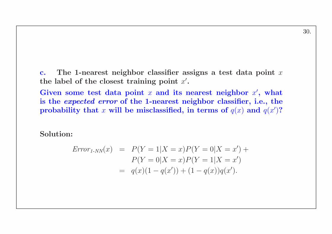
c. The 1-nearest neighbor classifier assigns a test data point xthe label of the closest training point x′.

Given some test data point x and its nearest neighbor x′, whatis the expected error of the 1-nearest neighbor classifier, i.e., theprobability that x will be misclassified, in terms of q(x) and q(x′)?

Solution:

Error1-NN(x) = P (Y = 1|X = x)P (Y = 0|X = x′) +

P (Y = 0|X = x)P (Y = 1|X = x′)

= q(x)(1− q(x′)) + (1− q(x))q(x′).

30.

d. In the asymptotic case, i.e. when the number of training ex-amples of each class goes to infinity, and the training data fillsthe space in a dense fashion, the nearest neighbor x′ of x has q(x′)converging to q(x), i.e. P (Y = 1|X = x′) → p(Y = 1|X = x).

(This is true due to i. the result obtained at the above point a, and

ii. the assumed continuity of the function py(x)not.= p(X = x|Y = y)

w.r.t. x.)

By performing this substitution in the expression obtained atpoint c, give the asymptotic error for the 1-nearest neighbor clas-sifier at point x, in terms of q(x).

Solution:limx′→x

Error1-NN(x) = 2q(x)(1− q(x))

31.

e. Show that the asymptotic error obtained at point d is less thantwice the Joint Bayes error obtained at point b and subsequentlythat this inequality leads to the corresponding relationship be-tween the expected error rates:

E[ limn→∞

Error1-NN] ≤ 2E[ErrorBayes].

Solution:

z(1− z) ≤ z for all z, in particular for z ∈ [0 , 1/2], andz(1− z) ≤ 1− z for all z, in particular for z ∈ [1/2 , 1].Therefore, for all x,

q(x)(1 − q(x)) ≤{

q(x) if q(x) ∈ [0 , 1/2]

1− q(x) if q(x) ∈ (1/2 , 1].

The results obtained at points b and d lead to

limn→∞

Error1-NN(x) = 2q(x)(1 − q(x)) ≤ 2ErrorBayes(x) for all x.

By multiplication with P (x) and suming upon all values of

x, we get: E[limn→∞ Error1-NN] ≤ 2E[ErrorBayes].

0

0.5

1

0 0.5 1z

2*min(z,1-z)min(z,1-z)

2*z-2*z2

z-z2

32.

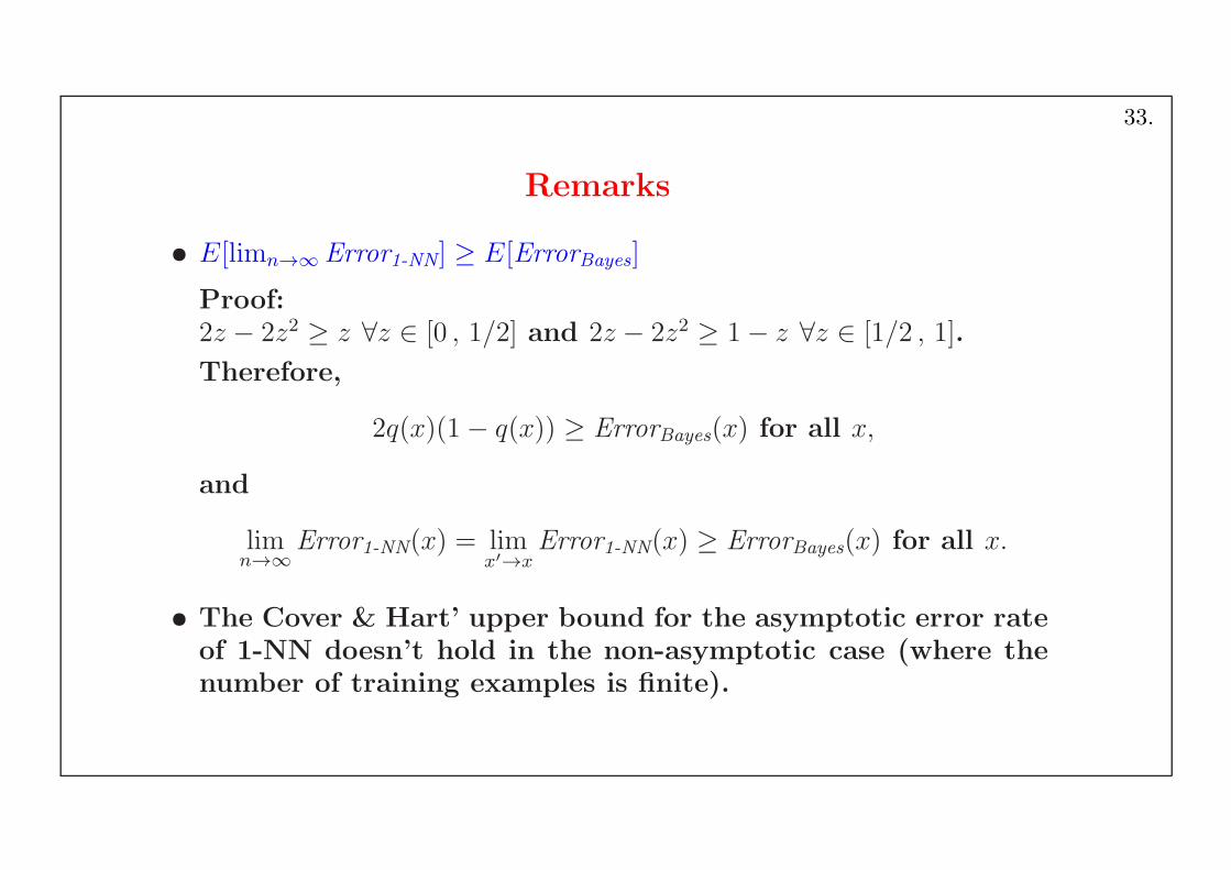
Remarks

• E[limn→∞ Error1-NN] ≥ E[ErrorBayes]

Proof:2z − 2z2 ≥ z ∀z ∈ [0 , 1/2] and 2z − 2z2 ≥ 1− z ∀z ∈ [1/2 , 1].

Therefore,

2q(x)(1− q(x)) ≥ ErrorBayes(x) for all x,

and

limn→∞

Error1-NN(x) = limx′→x

Error1-NN(x) ≥ ErrorBayes(x) for all x.

• The Cover & Hart’ upper bound for the asymptotic error rateof 1-NN doesn’t hold in the non-asymptotic case (where thenumber of training examples is finite).

33.

Remark

from: An Elementary Introduction to Statistical Learning Theory,

S. Kulkarni, G. Harman, 2011, pp. 68-69

An even tighter upper bound exists for E[limn→∞ Error1-NN]:2E[ErrorBayes](1 − E[ErrorBayes])

Proof:

From limx′→x Error1-NN(x) = 2q(x)(1− q(x)) (see point d) and

ErrorBayes(x) = min{1− q(x), q(x)} (see point b),

it follows thatlimx′

→x Error1-NN(x) = 2ErrorBayes(x)(1 − ErrorBayes(x)).

By multiplying this last equality with P (x) and suming on all x — in fact,integrating upon x —, we get

E[ limx′

→xError1-NN] = 2E[ErrorBayes(1− ErrorBayes)] = 2E[ErrorBayes]− 2E[(ErrorBayes)

2].

Since E[Z2] ≥ (E[Z])2 for any Z (Var(Z)def.= E[(Z−E[Z])2]

comp.= E[Z2]−(E[Z])2≥0),

it follows that

E[ limx′

→xError1-NN] ≤ 2E[ErrorBayes]− 2(E[ErrorBayes])

2 = 2E[ErrorBayes](1− E[ErrorBayes]).

34.

Other Results

[from An Elementary Introduction to Statistical Learning Theory,

S. Kulkarni, G. Harman, 2011, pp. 69-70]

• When certain restrictions hold,

E[ limn→∞

Errork-NN] ≤(

1 +1

k

)

E[ErrorBayes].

◦ However, it can be shown that there are some distributions for which1-NN outperforms k-NN for any fixed k > 1.

• Ifknn

→ 0 for n → ∞ (for instance, kn =√n), then

E[ limn→∞

Errorkn-NN] = E[ErrorBayes].

35.

Significance

The last result means that kn-NN is

− a universally consistent learner (because when the amount oftraining data grows, its performance approaches that of JointBayes) and

− non-parametric (i.e., the underlying distribution of data canbe arbitrary and we need no knowledge of its form).

Some other universally consistent learners exist.

However, the convergence rate is critical. For most learning meth-ods, the convergence rate is very slow in high-dimensional spaces(due to “the curse of dimensionality”). It can be shown that thereis no “universal” convergence rate, i.e. one can always find dis-tributions for which the convergence rate is arbitrarily slow.

There is no one learning method which can universally beat outall other learning methods.

36.

Conclusion

Such results make the ML field continue to be exciting,

and makes the design of good learning algorithms andthe understanding of their performance an importantscience and art!

37.

On 1-NN and kernelization with RBF

CMU, 2003 fall, T. Mitchell, A. Moore, final exam, pr. 7.f

38.

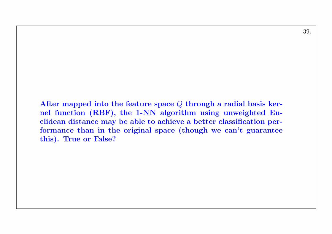
After mapped into the feature space Q through a radial basis ker-nel function (RBF), the 1-NN algorithm using unweighted Eu-clidean distance may be able to achieve a better classification per-formance than in the original space (though we can’t guaranteethis). True or False?

39.

Answer

Consider φ : Rd → Rn such that K(x, y)

not.= e−

||x−y||2

2σ2 = φ(x) ·φ(y), ∀x, y ∈ Rd. R

d is

the original space, Rn is the “feature” space, and e−||x−y||2

2σ2 is the radial basisfunction (RBF). Then

||φ(x) − φ(y)||2 = (φ(x) − φ(y)) · (φ(x) − φ(y))

= φ(x) · φ(x) + φ(y) · φ(y)− 2 · φ(x) · φ(y) = e−||x−x||2

2σ2 + e−||y−y||2

2σ2 − 2 · e−||x−y||2

2σ2

= e0 + e0 − 2 · e−||x−y||2

2σ2 = 2− 2 · e−||x−y||2

2σ2 = 2−K(x, y)

Suppose xi and xj are two neighbors for the test instance x such that ‖x−xi‖ <‖x− xj‖. After mapped to the feature space,

‖φ(x)− φ(xi)‖2 < ‖φ(x)− φ(xj)‖2 ⇔ 2−K(x, xi) < 2−K(x, xj) ⇔ K(x, xi) > K(x, xj)

⇔ e−||x−xi||

2

2σ2 > e−||x−xj ||

2

2σ2 ⇔ −||x− xi||22σ2

> −||x− xj ||22σ2

⇔ ||x− xi||2 < ||x− xj ||2.

So, if xi is the nearest neighbor of x in the original space, it will also be thenearest neighbor in the feature space. Therefore, 1-NN doesn’t work betterin the feature space. (The same is true for k-NN.)

Note: k-NN using non-Euclidean distance or weighted voting may work.

40.