Instability of high-frequency modes in viscoelastic plane Couette...

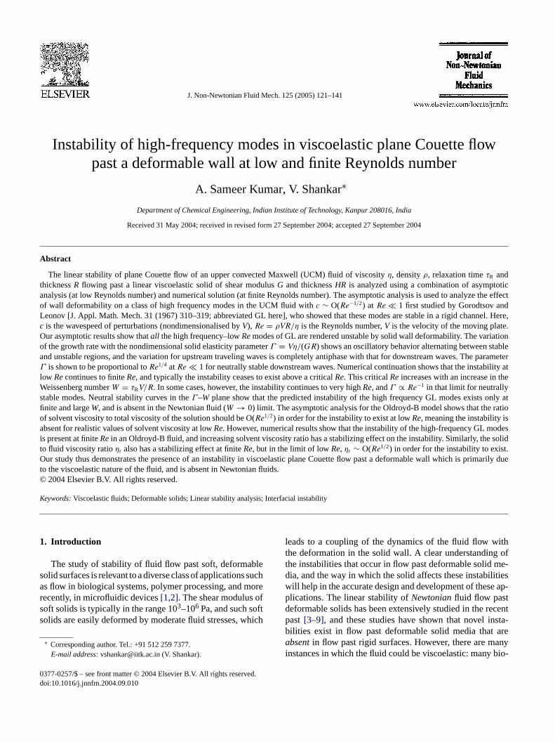
J. Non-Newtonian Fluid Mech. 125 (2005) 121–141

Instability of high-frequency modes in viscoelastic plane Couette flowpast a deformable wall at low and finite Reynolds number

A. Sameer Kumar, V. Shankar∗

Department of Chemical Engineering, Indian Institute of Technology, Kanpur 208016, India

Received 31 May 2004; received in revised form 27 September 2004; accepted 27 September 2004

Abstract

The linear stability of plane Couette flow of an upper convected Maxwell (UCM) fluid of viscosityη, densityρ, relaxation timeτR andthicknessR flowing past a linear viscoelastic solid of shear modulusG and thicknessHR is analyzed using a combination of asymptoticanalysis (at low Reynolds number) and numerical solution (at finite Reynolds number). The asymptotic analysis is used to analyze the effectof wall deformability on a class of high frequency modes in the UCM fluid withc ∼ O(Re−1/2) atRe � 1 first studied by Gorodtsov andLeonov [J. Appl. Math. Mech. 31 (1967) 310–319; abbreviated GL here], who showed that these modes are stable in a rigid channel. Here,c is the wavespeed of perturbations (nondimensionalised byV), Re = ρVR/η is the Reynolds number,V is the velocity of the moving plate.O ationo ablea parameterΓ ility atl heWs nly atfi ratioo sa odesi e solidt t.O marily duet©

K

1

sarss

ithofe-

itiesap-

centsta-areanybio-

0d

ur asymptotic results show thatall the high frequency–lowRemodes of GL are rendered unstable by solid wall deformability. The varif the growth rate with the nondimensional solid elasticity parameterΓ = Vη/(GR) shows an oscillatory behavior alternating between stnd unstable regions, and the variation for upstream traveling waves is completely antiphase with that for downstream waves. Theis shown to be proportional toRe1/4 atRe � 1 for neutrally stable downstream waves. Numerical continuation shows that the instab

ow Recontinues to finiteRe, and typically the instability ceases to exist above a criticalRe. This criticalReincreases with an increase in teissenberg numberW = τRV/R. In some cases, however, the instability continues to very highRe, andΓ ∝ Re−1 in that limit for neutrally

table modes. Neutral stability curves in theΓ–W plane show that the predicted instability of the high frequency GL modes exists onite and largeW, and is absent in the Newtonian fluid (W → 0) limit. The asymptotic analysis for the Oldroyd-B model shows that thef solvent viscosity to total viscosity of the solution should be O(Re1/2) in order for the instability to exist at lowRe, meaning the instability ibsent for realistic values of solvent viscosity at lowRe. However, numerical results show that the instability of the high-frequency GL m

s present at finiteRein an Oldroyd-B fluid, and increasing solvent viscosity ratio has a stabilizing effect on the instability. Similarly, tho fluid viscosity ratioηr also has a stabilizing effect at finiteRe, but in the limit of lowRe, ηr ∼ O(Re1/2) in order for the instability to exisur study thus demonstrates the presence of an instability in viscoelastic plane Couette flow past a deformable wall which is pri

o the viscoelastic nature of the fluid, and is absent in Newtonian fluids.2004 Elsevier B.V. All rights reserved.

eywords:Viscoelastic fluids; Deformable solids; Linear stability analysis; Interfacial instability

. Introduction

The study of stability of fluid flow past soft, deformableolid surfaces is relevant to a diverse class of applications suchs flow in biological systems, polymer processing, and moreecently, in microfluidic devices[1,2]. The shear modulus ofoft solids is typically in the range 103–106 Pa, and such softolids are easily deformed by moderate fluid stresses, which

∗ Corresponding author. Tel.: +91 512 259 7377.E-mail address:[email protected] (V. Shankar).

leads to a coupling of the dynamics of the fluid flow wthe deformation in the solid wall. A clear understandingthe instabilities that occur in flow past deformable solid mdia, and the way in which the solid affects these instabilwill help in the accurate design and development of theseplications. The linear stability ofNewtonianfluid flow pastdeformable solids has been extensively studied in the repast[3–9], and these studies have shown that novel inbilities exist in flow past deformable solid media thatabsentin flow past rigid surfaces. However, there are minstances in which the fluid could be viscoelastic: many

377-0257/$ – see front matter © 2004 Elsevier B.V. All rights reserved.oi:10.1016/j.jnnfm.2004.09.010

122 A.S. Kumar, V. Shankar / J. Non-Newtonian Fluid Mech. 125 (2005) 121–141

Nomenclature

c = cr + ici complex wave-speedG shear modulus of the solidH nondimensional thickness of the wallk wavenumberR dimensional thickness of fluidRe = RVρ/η Reynolds number of the flowV dimensional velocity of the top plateW = τRV/R Weissenberg number

Greek letters

β ratio of solvent to total viscosity in theOldroyd-B fluid

Γ = Vη/(GR) nondimensional solid elasticity param-eter

η viscosity of the fluidηr = ηw/η ratio of wall to fluid viscosityηw viscosity of the deformable solid wallτR relaxation time in the UCM model

logical fluids are non-Newtonian in nature and could exhibitviscoelastic behavior, and polymer solutions and melts are,of course, viscoelastic fluids. From a practical viewpoint, onemight envisage the use of deformable solid surfaces to induceinstabilities at low Reynolds number, and the resulting flowsmay provide a novel way of promoting mixing in viscoelasticfluids. From a fundamental standpoint, a pertinent questionis whether viscoelastic effects can induce additional modesof instabilities apart from those existent in Newtonian flowpast deformable solid media. A first step in this direction wastaken by Shankar and Kumar[10] who studied the stabilityof viscoelastic plane Couette flow past a deformable solid inthe creeping flow limit, but the instability they found was acontinuation of the already existent instability in Newtonianfluids modified by fluid viscoelastic effects. In this study, weuse both asymptotic and numerical methods to analyze the ef-fect of wall deformability on a class of high frequency modesfirst studied by Gorodtsov and Leonov[11] for plane Couetteflow of upper convected Maxwell fluid in a rigid channel.We predict here a new instability in viscoelastic plane Cou-ette flow past a deformable wall that is absent in Newtonianfluids. In the following discussion, we briefly recapitulaterelevant previous literature, and motivate the context for thepresent study.

Gorodtsov and Leonov[11] (abbreviated as GL in thispaper) first analyzed the stability of plane Couette flow ofa fter)fl s ofm hei flowl att peed

In this paper, we refer to these two discrete eigenvalues as‘zero Reynolds number GL modes’, and this is henceforthabbreviated as ZRGL modes. (There also exists a continu-ous spectrum of eigenvalues[12], which are always stable,and we restrict our discussion only to the discrete part of thespectrum.) (2) In Section3 of their paper, GL analyzed thestability problem in theRe � 1 limit, but with wave speedc ∼ Re−1/2 1 (if the Weissenberg numberW ∼ O(1)).This corresponds to very high frequency of oscillations ofthe perturbations in the limit of lowRe. In this limit, some ofthe inertial terms in the governing stability equation for thefluid cannot be neglected despite theRe � 1 limit. GL car-ried out an asymptotic analysis in the small parameterRe1/2

and calculated the wavespeed as an asymptotic series. Theirresults show that there aremultiple solutionsto the leadingorder wavespeed, all of which are real. Consequently, thefirst correction to the wavespeed determines the stability ofthe system, which they demonstrate to be stable for all thesolutions. These results are valid in the limitRe � 1. Werefer to these solutions as the ‘high frequency GL modes’,and this is abbreviated as HFGL in the following discussion.Physically, for perturbations at high frequencies (comparedto the shear rate of the base Couette flow), the UCM fluidbehaves similar to an elastic solid, and the HFGL modes ina UCM fluid are essentially identical to shear waves in anelastic solid[13]. The wavespeed of shear waves in an elastics so od-ua vesnt peeda hes dis-c cya d byt classo per)a ei ardy[ thisl

od byR u-e ofd iono dis-c ationo RGLm ytf ris[ asticpf

n upper convected Maxwell (abbreviated UCM hereauid in rigid channels. GL essentially analyzed two typeodes: (1) In Section2 of their paper, they neglected t

nertial terms in the fluid and considered the creepingimit (Reynolds numberRe = 0), where they showed thhere are two stable discrete eigenvalues for the waves
.
olid is proportional to√G/ρ whereG is the shear modulu

f the solid andρ is the density. If we estimate the elastic mlus of the UCM fluid (with viscosityη, relaxation timeτRnd densityρ) as

√η/τR, then the dimensional shear wa

peed for a UCM fluid is proportional to√η/(τRρ). Upon

ondimensionalising this wavespeed with the velocityV inhe Couette flow, one obtains the nondimensional wavess c ∝ Re−1/2W−1/2 for elastic shear waves, which is tcaling assumed by GL in their analysis. Therefore, therete solutions toc obtained by GL in their high-frequennalysis are elastic shear waves in a UCM fluid modifie

he presence of the Couette flow. Apart from these twof modes, they also carry out (in Section 4 of their pan asymptotic analysis in the limitkW 1, and concludncorrectly (proved subsequently by Renardy and Ren14]) that the UCM plane Couette flow is unstable inimit.

Subsequent numerical analysis using a spectral methenardy and Renardy[14] showed that the UCM plane Cotte flow is always stable at finiteRe, and they reported a setiscrete eigenvalues from their spectral method. In Sect3f this paper, we show that these numerically computedrete spectrum of eigenvalues are nothing but a continuf the HFGL modes (discussed above) and the two Zodes to finiteRe. Renardy[15] further proved rigorousl

hat the UCM plane Couette flow isstableat Re = 0, andor arbitrary values ofW. Similarly, Sureshkumar and Be16] showed using a numerical method that the viscoellane Poiseuille flow of a UCM fluid is also stable atRe = 0

or all W. The earlier study of Ho and Denn[17] analyzed

A.S. Kumar, V. Shankar / J. Non-Newtonian Fluid Mech. 125 (2005) 121–141 123

the stability of plane Poiseuille flow of an UCM fluid in rigidchannels using a numerical shooting procedure, and showedthat the flow is stable at lowReand finiteW. Wilson et al.[12] studied the spectrum for UCM and Oldroyd-B fluids atRe = 0 in both plane Couette and combined Couette-planePoiseuille configurations. They showed how the discretespectrum changes as the Couette flow is changed to a planePoiseuille flow and also as the constitutive model is changedfrom UCM to Oldroyd-B fluid. All these previous studies,however, analyzed the stability of viscoelastic flow in rigidchannels.

Shankar and Kumar[10] recently studied the effect of walldeformability on the two ZRGL modes in the creeping flowlimit, where the inertial effects in the fluid and the solid wereneglected. At fixed Weissenberg numberW, they showed thatone of the two discrete stable ZRGL modes becomes unstableupon increase of the nondimensional solid elasticity param-eterΓ = Vη/(GR) above a critical value. However, whenneutral stability curves were constructed in theΓ–W plane,they found that this unstable mode continues to the limit ofW → 0 (Newtonian fluid), and in this limit, it reduces to theNewtonian fluid instability past a deformable wall first stud-ied by Kumaran et al.[3]. Thus, the continuation of the sta-ble ZRGL modes to finite wall deformability gives the sameunstable mode as the continuation of the unstable mode ofKumaran et al. to finite Weissenberg number. Therefore, thee notg t am dsb CMfl bil-i hent inc

eH sn studyFR theR tsi thisc fluida hicha ce ot earw y oft d. TotW tyo teu ber’E

oaTt ion

of the previous zero-Reinstability of Shankar and Kumar[10]to finiteRewith the present results.

The primary objective of the present study is to quali-tatively demonstrate the presence of a new class of unstablemodes in viscoelastic flow past deformable solid surfaces dueto the elastic nature of the fluid, and the simple UCM modelsuffices for this purpose. However, some preliminary numer-ical results for the Oldroyd-B model (which adds a solventviscosity contribution to the UCM model) are also presented,in order to show that the predicted instability could be po-tentially observed even in the presence of nonzero solventviscosity. Despite the use of these simple models to describethe viscoelastic fluid, it is expected that the present instabil-ity should exist even in more realistic models for polymersolutions and melts.

The rest of this paper is organized as follows. In Sec-tion2, we develop the governing linear stability equations andboundary conditions, and also describe and validate the nu-merical method used to solve the coupled fluid–solid stabilityequations. In Section3, we demonstrate that the numericallycomputed discrete spectrum for UCM plane Couette flow inrigid channels[14] is nothing but a finite-Recontinuation ofthe ZRGL and HFGL modes first analyzed by GL. Section4.1presents the asymptotic analysis for UCM Couette flow pasta deformable wall, and also the results from the analysis inthe limit Re � 1. Section4.2 provides some representative

-the

olid-k-

ple,cos-e-ded

ional)

ffect of wall deformability on the ZRGL modes doesive rise to a qualitatively new instability, rather it is jusodification of the instability existing in Newtonian fluiy fluid viscoelastic effects. The elastic nature of the Uuid has a stabilizing effect on the Newtonian fluid instaty, and the instability ceases to exist in the UCM fluid whe nondimensional groupτRG/η is greater than a certaritical value.

The effect of wall deformability on the stability of thFGL class of solutions studied by GL[11], however, haot been analyzed, and this is the subject of the presentor the HFGL class of modes,c ∼ Re−1/2 in the limit of lowe, so inertial effects in the fluid come into play even ine � 1 limit. One might similarly expect the inertial effec

n the deformable solid also to become important forlass of modes. In the absence of flow, both the UCMnd the elastic solid will admit elastic shear waves, wre stable due to viscous effects in the fluid. The presen

he plane Couette flow in the fluid will modify these shaves, and we analyze how the flow affects the stabilit

he shear waves when the fluid flows past an elastic solihis end, we first use an asymptotic analysis in theRe � 1,

∼ O(1) limit to examine the effect of wall deformabilin the HFGL modes, and we continue these results to finiResing a numerical method. In terms of the ‘elasticity num≡ W/Re often used to characterize viscoelastic flows[16],

ur asymptotic analysis corresponds to the limit ofE 1,nd the small parameter of our asymptotic analysis isE−1/2.he numerical results extend the asymptotic results atE 1

o finite values ofE ∼ O(1). We also contrast the continuat

.

f

numerical results at finiteRefor both the UCM and OldroydB models. Section5 summarizes the salient results frompresent study.

2. Problem formulation and numerical method

2.1. Governing equations

The system of interest consists of a linear viscoelastic sof thicknessHRand shear modulusG fixed onto a rigid surface atz∗ = −HR, and a layer of viscoelastic fluid of thicnessR in the region 0< z∗ < R (seeFig. 1). The viscoelasticfluid is modeled using the UCM model (see, for exam[18]), which has two material constants: a constant visity η and a relaxation timeτR. In what follows, we denotdimensional variables with a superscript∗ and nondimensional variables without any superscript. The fluid is boun

Fig. 1. Schematic diagram showing the configuration and (nondimenscoordinate system considered in this paper.


at z∗ = R by a rigid plate which moves at a constant veloc-ity V in thex-direction relative to the deformable solid wall.The following scales are used for nondimensionalising vari-ous quantities at the outset:R for lengths and displacements,V for velocities,R/V for time, andηV/R for stresses andpressure. Thus,H is the nondimensional thickness of the de-formable solid layer.

The nondimensional equations governing the dynamics ofthe fluid are the mass and momentum conservation equations:

∂ivi = 0, Re[∂t + ∂jvj]vi = ∂jTij. (1)

Here, vi is the velocity field in the fluid,Re = ρVR/η isthe Reynolds number in the fluid,Tij = −pf δij + τij is thetotal stress tensor in the fluid which is a sum of an isotropicpressure−pf δij and the extra-stress tensorτij, and the indicesi andj can take the valuesx, z. The extra-stress tensor is givenby the UCM constitutive relation as:

W [∂tτij + vk∂kτij − ∂kviτkj − ∂kvjτki] + τij=(∂ivj + ∂jvi),

(2)

where ∂t ≡ (∂/∂t), ∂i ≡ (∂/∂xi), and W = τRV/R is theWeissenberg number characterizing the relaxation time ofthe viscoelastic fluid. No-slip conditions are appropriate forthe velocity field in the fluid atz = 1:

v

w d thed

ess-i evi-o ,G s ofu thes thes all.T ands ara allv thec lsop cialt d tot keans vis-c thatt ts fort d bya t oft e ve-li emenfi

∂

The momentum conservation equation in the solid layer isgiven by

Re ∂2t ui = ∂jΠij, (5)

whereΠij = −pgδij + σij is the total stress tensor in the solidwhich is given by a sum of the isotropic pressure−pgδij andthe deviatoric stress tensorσij. Without loss of generality, wehave set the density of the solid equal to the density of thefluid ρ. The deviatoric stressσij is given by a sum of elasticand viscous stresses in the deformable solid:

σij =(

1

Γ+ ηr∂t

)(∂iuj + ∂jui), (6)

whereΓ = Vη/(GR) is the nondimensional parameter char-acterizing the elasticity of the solid layer, andηr = ηw/η

is the ratio of wall to fluid viscosities. The nondimensionalgroupΓ is the estimated ratio of viscous stresses in the fluidto elastic stresses in the solid layer. The solid layer is assumedto be fixed to a rigid surface atz = −H , and so the boundarycondition there isui = 0.

The conditions at the interfacez = h(x) between the fluidand the deformable solid wall are the continuity of velocitiesand stresses:

vi = ∂tui, Tijnj = Πijnj, (7)

wF ndi-t conde rs.W solidl tressc

2

ofilew aneC

v

τ

A e andi zerofi ti ll isa unidi-r hei

u

σ

T ate.

x = 1, vz = 0, (3)

hile the conditions at the interface between the fluid aneformable solid wall are discussed below.

The deformable solid wall is modeled as an incomprble linear viscoelastic solid, similar to that used in the prus studies in this area (see, for example,[3,4,10]). Recentlykanis and Kumar[19] have examined the consequencesing a nonlinear model for describing the deformation inolid wall, by using the neo-Hookean model for analyzingtability of creeping Newtonian flow past a deformable whis study has shown that for nonzero interfacial tensionufficiently large values ofH, the results from both linend nonlinear solid models agree quite well, while for smalues ofH < 2, the linear model somewhat overpredictsritical velocity required for destabilizing the flow. They aredict a shortwave instability in the absence of interfa

ension at the solid–fluid interface, and this was attributehe nonzero first normal stress difference in the neo-Hooolid. In this study, we restrict ourselves to the linearoelastic solid model, and it is argued later in this paperhe linear solid model is expected to yield accurate resulhe present instability. The deformable solid is describedisplacement fieldui which represents the displacemen

he material points from their steady-state positions. Thocity field in the wall medium isvi = ∂tui. The solid mediums assumed to be incompressible, and hence the displaceld satisfies the solenoidal condition:

iui = 0. (4)

t

herenj is the unit normal to the interfacez = h(x) (seeig. 1). The normal and tangential stress continuity co

ions at the interface are obtained by contracting the sequation in Eq.(7) with the unit normal and tangent vectohen the interfacial tension between the fluid and the

ayer is nonzero, additional terms appear in the normal sontinuity.

.2. Base state

The steady, unidirectional base state velocity prhose stability is of interest in this study is simply the plouette flow profile:

x = z, vz = 0,

xx = 2W, τzz = 0, τxz = τzx = 1. (8)

ll the base flow quantities are denoted by an overbar hern the following discussion. Note the presence of a nonrst normal stress differenceτxx − τzz = 2W which is absenn the case of Newtonian fluids. The deformable solid wat rest in this steady base state, but there is a nonzeroectional displacement field ¯ux due to the fluid stresses at tnterface:

x = Γ (z + H), uz = 0,

xx = σzz = 0, σxz = σzx = 1. (9)

he fluid–solid interface is uniform and flat in this base st


2.3. Linear stability analysis

A temporal linear stability analysis is used to determinethe stability of the above base state, where small perturba-tions (denoted by primed quantities) are introduced to thefluid velocity field about the base statevi = vi + v′

i, and otherdynamical quantities in the fluid and the solid are similarlyperturbed. The perturbation quantities are expanded in theform of Fourier modes in thex-direction, and with an expo-nential dependence in time:

v′i = vi(z) exp[ik(x − ct)], u′

i = ui(z) exp[ik(x − ct)],

(10)

wherek is the wavenumber,c is the complex wavespeed, andvi(z) and ui(z) are eigenfunctions which have to be deter-mined from the linearized governing equations and boundaryconditions. The complex wavespeed is given byc = cr + iciand whenci > 0, the base state is temporally unstable.

Upon substituting the above form for the perturbationsin the governing equations(1) and the constitutive relationfor the UCM fluid (2), we obtain the following linearizedgoverning equations (where dz = d/dz):

dzvz + ikvx = 0, (11)

−−{{

{

F if-f

{

wthe

ds

d

−

−

These equations can be reduced to a single fourth-order dif-ferential equation for ˜uz:

(d2z − k2)

[d2z − k2

(1 − ΓRe c2

1 − ikcηrΓ

)]uz = 0. (21)

The linearized boundary conditions at the unperturbed in-terface positionz = 0 between the fluid and the solid layerare obtained by Taylor-expanding about the flat interface po-sition in the base state[3,10]:

vz = (−ikc)uz, (22)

vx + uz = (−ikc)ux, (23)

−pf + τzz − Σk2uz = −pg + 2

(1

Γ− ikcηr

)dzuz, (24)

τxz − 2ikWuz =(

1

Γ− ikcηr

)(dzux + ikuz). (25)

Here,Σ = γ/(ηV ) is the nondimensional parameter charac-terizing the interfacial tension (γ) between the fluid and thesolid layer. The second term in the left side of Eqs.(23) and(25)represent nontrivial contributions that arise as a result ofthe Taylor expansion of the mean flow quantities about theunperturbed interface. The term in Eq.(23) arises due to thediscontinuity in the gradient of the base flow velocity profileat the interface, while the term in Eq.(25) arises due to thed thefl s atz

v

w

u

Tv on-d a-b fR

nn blemi

2s for

a yβ s-i ares dis-c ity.T l-vm r theO

d

ikpf + ikτxx + dzτxz = Re[ik(z − c)vx + vz], (12)

dzpf + dzτzz + ikτxz = Re[ik(z − c)vz], (13)

1 + ikW(z − c)}τzz = 2dzvz + 2ikWvz, (14)

1 + ikW(z − c)}τxz= (dzvx + ikvz) + W(τzz + 2ikW vz), (15)

1 + ikW(z − c)}τxx= 2ikvx + W(2τxz + 4ikWvx + 2dzvx). (16)

ollowing[11], we obtain a single fourth-order ordinary derential equation (ODE) forvz from the above equations:

ξ2d2z − 2ξdz + 2 − k2ξ2}{d2

z + 2ikWdz − k2(1 + 2W2)}vz= −k2W Re ξ3(z − c)[d2

z − k2]vz, (17)

here the variableξ is defined asξ = [z − c − i/(kW)].The governing equations for the displacement field in

eformable solid wall can be expressed in terms of ˜ui(z) in aimilar manner to give:

zuz + ikux = 0, (18)

ikpg +(

1

Γ− ikcηr

)(d2

z − k2)ux = −Re k2c2ux, (19)

dzpg +(

1

Γ− ikcηr

)(d2

z − k2)uz = −Re k2c2uz. (20)

iscontinuity of the first normal stress difference betweenuid and the deformable solid. The boundary condition= 1 are simply

˜z = 0, vx = 0, (26)

hile the boundary conditions atz = −H are

˜ z = 0, ux = 0. (27)

he two fourth order differential equations(17) and (21)for˜z anduz along with the eight interface and boundary citions (Eqs.(22)–(27)) completely specify the linear stility problem. The complex wavespeedc is a function oe,W, Γ, ηr, k,Σ andH. For arbitrary values ofRe, there iso closed form solution to the fourth order Eq.(17), and so aumerical method must be used to solve the stability pro

n general.

.3.1. Linear stability equations for Oldroyd-B fluidIn this section, we present the linear stability equation

n Oldroyd-B fluid of total viscosityη, and solvent viscositη, whereβ is the ratio of solvent viscosity to total visco

ty of the polymer solution. The nondimensional scalesimilar to those used for the UCM fluid in the precedingussion, withη taking the meaning of the total fluid viscoshe extra-stress tensorτij is comprised of the Newtonian soent part and the polymer part:τij = τs

ij + τpij. The linearized

omentum equations and the constitutive relations foldroyd-B fluid are given by:

zvz + ikvx = 0, (28)


Re[ik(z − c)vx + vz]

= −ikpf + β(d2z − k2)vx + ikτp

xx + dzτpxz, (29)

Re[ik(z − c)vz]

= −dzpf + β(d2z − k2)vz + dzτ

pzz + ikτp

xz, (30)

{1 + ikW(z − c)}τpzz = 2(1− β)dzvz + 2ikW(1 − β)vz,

(31)

{1 + ikW(z − c)}τpxz

= (1 − β)[dzvx + ikvz + 2W2ik vz] + Wτpzz, (32)

{1 + ikW(z − c)}τpxx

= (1 − β)[2ikvx + W(4ikWvx + 2dzvx)] + 2Wτpxz. (33)

The base state quantities for the Oldroyd-B fluid are iden-tical to that for the UCM fluid (Eq.(8)), except for the nor-mal stressτxx, which is given byτxx = 2(1− β)W for theOldroyd-B fluid. The boundary conditions at the interfacez = 0 are identical to those for the UCM fluid (Eqs.(22)–(27)), with the understanding thatτij is the sum of polymerand solvent stress in the Oldroyd-B fluid, and the secondterm in the left side of Eq.(25)acquires a coefficient (1− β)dfl

2

er-i atedi dents ryc nts d-a ford urtho ntrola ure,s ianfl lda fouria ma-tR thes

m-p allt d ini-t ently,a nval-u w-e low

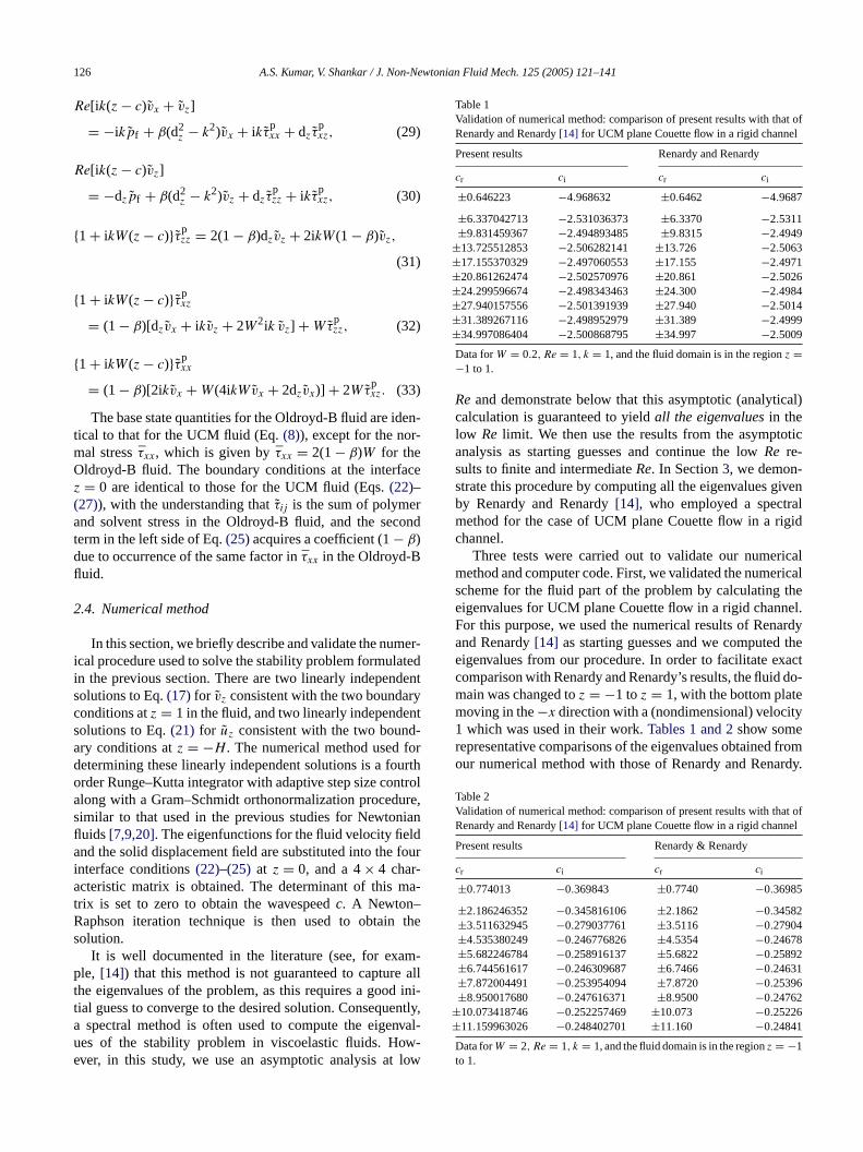
Table 1Validation of numerical method: comparison of present results with that ofRenardy and Renardy[14] for UCM plane Couette flow in a rigid channel

Present results Renardy and Renardy

cr ci cr ci

±0.646223 −4.968632 ±0.6462 −4.9687

±6.337042713 −2.531036373 ±6.3370 −2.5311±9.831459367 −2.494893485 ±9.8315 −2.4949

±13.725512853 −2.506282141 ±13.726 −2.5063±17.155370329 −2.497060553 ±17.155 −2.4971±20.861262474 −2.502570976 ±20.861 −2.5026±24.299596674 −2.498343463 ±24.300 −2.4984±27.940157556 −2.501391939 ±27.940 −2.5014±31.389267116 −2.498952979 ±31.389 −2.4999±34.997086404 −2.500868795 ±34.997 −2.5009

Data forW = 0.2, Re = 1, k = 1, and the fluid domain is in the regionz =−1 to 1.

Reand demonstrate below that this asymptotic (analytical)calculation is guaranteed to yieldall the eigenvaluesin thelow Re limit. We then use the results from the asymptoticanalysis as starting guesses and continue the lowRe re-sults to finite and intermediateRe. In Section3, we demon-strate this procedure by computing all the eigenvalues givenby Renardy and Renardy[14], who employed a spectralmethod for the case of UCM plane Couette flow in a rigidchannel.

Three tests were carried out to validate our numericalmethod and computer code. First, we validated the numericalscheme for the fluid part of the problem by calculating theeigenvalues for UCM plane Couette flow in a rigid channel.For this purpose, we used the numerical results of Renardyand Renardy[14] as starting guesses and we computed theeigenvalues from our procedure. In order to facilitate exactcomparison with Renardy and Renardy’s results, the fluid do-main was changed toz = −1 toz = 1, with the bottom platemoving in the−x direction with a (nondimensional) velocity1 which was used in their work.Tables 1 and 2show somerepresentative comparisons of the eigenvalues obtained fromour numerical method with those of Renardy and Renardy.

Table 2Validation of numerical method: comparison of present results with that ofRenardy and Renardy[14] for UCM plane Couette flow in a rigid channel

P

c

±±Dt

ue to occurrence of the same factor inτxx in the Oldroyd-Buid.

.4. Numerical method

In this section, we briefly describe and validate the numcal procedure used to solve the stability problem formuln the previous section. There are two linearly indepenolutions to Eq.(17) for vz consistent with the two boundaonditions atz = 1 in the fluid, and two linearly independeolutions to Eq.(21) for uz consistent with the two bounry conditions atz = −H . The numerical method usedetermining these linearly independent solutions is a forder Runge–Kutta integrator with adaptive step size colong with a Gram–Schmidt orthonormalization procedimilar to that used in the previous studies for Newtonuids[7,9,20]. The eigenfunctions for the fluid velocity fiend the solid displacement field are substituted into the

nterface conditions(22)–(25)at z = 0, and a 4× 4 char-cteristic matrix is obtained. The determinant of this

rix is set to zero to obtain the wavespeedc. A Newton–aphson iteration technique is then used to obtainolution.

It is well documented in the literature (see, for exale, [14]) that this method is not guaranteed to capture

he eigenvalues of the problem, as this requires a gooial guess to converge to the desired solution. Consequ

spectral method is often used to compute the eigees of the stability problem in viscoelastic fluids. Hover, in this study, we use an asymptotic analysis at

resent results Renardy & Renardy

r ci cr ci

±0.774013 −0.369843 ±0.7740 −0.36985

±2.186246352 −0.345816106 ±2.1862 −0.34582±3.511632945 −0.279037761 ±3.5116 −0.27904±4.535380249 −0.246776826 ±4.5354 −0.24678±5.682246784 −0.258916137 ±5.6822 −0.25892±6.744561617 −0.246309687 ±6.7466 −0.24631±7.872004491 −0.253954094 ±7.8720 −0.25396±8.950017680 −0.247616371 ±8.9500 −0.2476210.073418746 −0.252257469 ±10.073 −0.2522611.159963026 −0.248402701 ±11.160 −0.24841

ata forW = 2, Re = 1, k = 1, and the fluid domain is in the regionz = −1o 1.


This comparison shows that our results agree very well withthe previous results of Renardy and Renardy. It should benoted that there exist solutions[14] with the same imaginarypartci and with real partcr having the same magnitude butwith opposite signs. Secondly, in order to validate the nu-merical procedure for the combined fluid–solid problem atfiniteRe, we compared the results obtained from our methodfor W → 0 with the previous numerical results of Srivatsanand Kumaran[20] who studied the stability of plane Couetteflow of a Newtonian fluid, and again excellent agreementwas obtained. Thirdly, we also compared the results obtainedfrom our method in theRe → 0 limit, but at finiteW, withthose of Shankar and Kumar[10], who obtained analyticalsolutions for the stability of UCM Couette flow past a de-formable wall in the creeping flow limit, and found very goodagreement.

3. Structure of stable modes at low and finiteRe forUCM plane Couette flow in a rigid channel

In this section, we demonstrate that the eigenvalues of thediscrete spectrum for UCM plane Couette flow in rigid chan-nels computed by Renardy and Renardy[14] atRe ∼ O(1)are essentially a finite-Recontinuation of the high frequency–low Reand zeroRestable modes of Gordotsov and Leonov[t pa-r totics sts dingo ly,t m,w ons.T -t fromtt ea uid.T odesi ardy[t GLm thes bled od.

theH ent des ofR dG onlyt -a sisi Lm e re-

Table 3The first nine modes for the leading order wavespeedc(0) calculated fromGL’s high frequency asymptotic analysis

W = 0.2 W = 2

±6.82068 ±2.26768±10.1611 ±3.54169±13.954 ±4.5692±17.3403 ±5.69414±21.0114 ±6.75548±24.4292 ±7.87805±28.0522 ±8.95583±31.4893 ±10.0774±35.0865 ±11.1639

Data fork = 1, Re � 1. The fluid domain ranges fromz = −1 to 1.

sults for a rigid channel. In order to facilitate the comparisonwith the results of Renardy and Renardy, the fluid domainranges fromz = −1 to 1, and the bottom rigid plate has avelocity −1. The first correction was not required becausethe leading order wavespeed was found to be a sufficientlygood initial guess for our numerical procedure. The char-acteristic equation admits multiple solutions toc(0), all ofwhich are real. The first few solutions to the leading orderwavespeed obtained from the asymptotic analysis are dis-played inTable 3. For ease of discussion, we designate num-bers to the various solutions based on increasing magnitude ofc(0), i.e., the solution with the lowest magnitude ofc(0) is re-ferred to as ‘mode 1’, and increasing mode numbers are givento solutions with increasing magnitudes ofc(0). There existsolutions forc(0) with the same magnitude but with oppo-site signs, and these two solutions correspond to downstream(c(0) positive) and upstream (c(0) negative) traveling waves inthe system. The leading order solutions forc(0) are providedas starting guesses at lowRe(sayRe = 10−4) to the numer-ical procedure described previously, and these solutions arecontinued to finiteRe.

The numerical solutions toc show that it is a complexquantity, and has anegativeimaginary part indicating thatthe flow is stable in this limit for this class of modes. Also,for each mode, there are two solutions corresponding to up-stream and downstream traveling waves (having the samemt3m ntly,wa esi twoc nt e tofi tin-u bydTa s,t oft s.

11]. GL carried out an asymptotic analysis (see Section1 ofhis paper for a brief review of GL’s analysis) in the smallameterRe1/2 and calculated the wavespeed as an asymperies. If we stipulate thatW ∼ O(1), GL’s asymptotic serieakes the formc = Re−1/2(c(0) + Re1/2 c(1) + · · ·). Their re-ults show that there are multiple solutions to the learder wavespeedc(0), all of which are real. Consequent

he first correctionc(1) determines the stability of the systehich they demonstrate to be stable for all the solutihese results are valid in the limitRe � 1, and these solu

ions are referred to as HFGL modes in this paper. Aparthese high frequency solutions in the lowRelimit, there arewo solutions to the wavespeed for whichc ∼ O(1) and thesre obtained by neglecting the inertial effects in the flhese two discrete modes are referred to as the ZRGL m

n this paper. The numerical results of Renardy and Ren14] (shown inTables 1 and 2in this paper) at finiteReshowhat the first eigenvalue corresponds to the pair of ZRodes (withcr having positive and negative values, and

ameci ). At finiteRe, they reported a number of other staiscrete eigenvalues computed from their spectral meth

We were interested in examining the evolution ofFGL modes to finiteRe, and the connection (if any) betwe

hese stable modes and the numerically determined moenardy and Renardy[14] at finite values ofRe. We repeateL’s high frequency asymptotic analysis and calculated

he leading order wavespeedc(0) using the symbolic packgeMathematica. We briefly outline the asymptotic analy

n Section4.1 in the context of the stability of these HFGodes past a deformable wall. Here, we merely state th

agnitude but opposite signs for the real part ofc), but bothhese solutions have the same negativeci value.Figs. 2 and

show the evolution ofc with Re for the first few HFGLodes obtained from the asymptotic analysis. Importae find that the continuation of the HFGL solutions forc(0)

t lowReto Re = 1 yields all the numerically found modn Renardy and Renardy’s analysis shown in the firstolumns ofTables 1 and 2, except for the very first row ihese tables which is a continuation of the ZRGL modnite Re. Indeed, even without doing the numerical conation to finiteRe, it is possible to see the connectionirectly comparing theRe → 0 asymptotic result forc(0) inable 3with theRe = 1 numerical result forcr in Tables 1nd 2. SinceRe = 1 (and soRe−1/2 = 1) in these table

he asymptotic result forc(0) is in fact the actual real parthe wavespeed predicted by the lowReasymptotic analysi


Fig. 2. Continuation of the first few high-frequency GL modes from lowReto finiteRein a rigid channel. Data forW = 0.2, k = 1 for the configuration−1 ≤ z ≤ 1 with the lower rigid plate moving in the opposite direction. (a)cr vs.Re; (b) ci vs.Re.

The first row in theTables 1 and 2correspond to theRe = 0GL (ZRGL) mode, and the real parts of all the rest of themodes in these tables are quite close to the asymptotic re-sults inTable 3, despite the fact that the numerical results arefor Re = 1. We have also verified that the other set of datafor k = 15,W = 1, Re = 0.25 presented in Renardy and Re-nardy’s paper are also a continuation of the high frequencyGL modes. Therefore, this comparison suggests that all thestable discrete modes for the UCM plane Couette flow prob-lem at finiteRewere already present in GL’s paper, albeit inthe lowRelimit. To the best of our knowledge, this connec-tion between the ZRGL and HFGL modes at lowReand thediscrete modes computed numerically at finiteRe [14] hasnot been made explicit in the literature on the linear stabilityof UCM plane Couette flow. With the aid of both the zeroReanalysis and the low-Re, high frequency asymptotic analysis

Fig. 3. Continuation of the first few high-frequency GL modes from lowReto finiteRein a rigid channel. Data forW = 2, k = 1 for the configuration−1 ≤ z ≤ 1 with the lower rigid plate moving in the opposite direction. (a)cr vs.Re; (b) ci vs.Re.

of GL, it is therefore possible to generateall the discrete sta-ble modes for UCM plane Couette flow in rigid channels atlow Re, and the numerical procedure outlined in Section2.4can be used to continue these solutions to any desired finiteRe.

It is useful here to remark on the nature of the modes forUCM Couette flow in a rigid channel if the fluid domain ischanged to 0≤ z ≤ 1, and if the bottom rigid wall atz = 0 isstationary. In that case, the two discrete ZRGL modes have thesameci (negative) value, but with very differentcr values. Forthe domain used by Renardy and Renardy[14] wherez = −1to z = 1, with the bottom plate moving with a velocity−1,the two discrete ZRGL modes have the same negativeci valueand with real partcr having the same magnitude but oppositesigns. For the HFGL class of modes, however, in the domainz = 0 toz = 1 with thez = 0 boundary being stationary, the


numerical solutions show that for each mode there are twosolutions withcr having very nearly the same magnitude (theagreement improves asRe � 1) and opposite signs, and withthe same (negative) value ofci . For the configuration used byRenardy and Renardy, for each mode there are two solutionswith cr having exactly the same magnitude even at finiteRe.

4. Effect of wall deformability on high frequency GLmodes

In this section, the effect of wall deformability on theHFGL modes is examined first using an asymptotic analysisin the limitRe � 1, and then using the numerical proceduredescribed in Section2.4.

4.1. Asymptotic analysis at low Re

Following Section3 of GL [11], we consider the limitRe � 1, andc ∼ Re−1/2 1. In the original GL analysis,the relevant small parameter was (Re/W)1/2. However, inthe present analysis, we considerW ∼ O(1), and so the ap-propriate small parameter is simplyRe1/2. The wavespeed istherefore expanded in an asymptotic series:

c = Re−1/2c(0) + c(1) + · · · . (34)

I suf-fiU or-d isl

{

A ntk s int

v

v

t (Eqs.( ses:

τ

τ

τ

Tm d as:

p

Upon substituting the above expansions in the Eqs.(12)–(16), we obtain the following simplified expressions for thestresses and the pressure to leading order:

−ikWc(0)τ(0)zz = 2dzv

(0)z + 2ikWv(0)

z , (41)

−ikWc(0)τ(0)xz = (dzv

(0)z + ikv(0)

z ) + 2ikW2v(0)z , (42)

−ikWc(0)τ(0)xx = 2ikv(0)

x + 4ikW2v(0)x + 2Wdzv

(0)x , (43)

−ikp(0)f = −ikc(0)v(0)

x − ikτ(0)xx − dzτ

(0)xz . (44)

Comparing these simplified leading order equations forc ∼Re−1/2 1 with the original set of Eqs.(14)–(16), it is clearthat only the ‘elastic part’ of the left side of these equationsmanifest in this limit. This is because the high frequency per-turbations under consideration here ‘probe’ only the elasticnature of the viscoelastic fluid to leading order in the analysis.

The velocity continuity conditions(22) and (23)sug-gest the expansions for the solid displacement field: sincevz ∼ Re−1/2, uz ∼ O(1) becausec ∼ Re−1/2. Therefore, thedisplacement and pressure fields in the solid layer are ex-panded as follows:

uz = u(0)z + Re1/2 u(1)

z + · · · , (45)

ux = u(0)x + Re1/2 u(1)

x + · · · , (46)

p

E tics esses,tT -tw inge

d

−

−

S s int en int tst orderd

(

n the present study, further analysis indicates that it iscient to calculate only the leading order wavespeedc(0).pon substituting this expansion in the governing fourther ODE for the fluid(17), the leading order equation in th

imit becomes:

d2z − k2}{d2

z + 2ikWdz + k2[(c(0))2W − 1 − 2W2]}vz = 0.

(35)

lthough Re � 1, sincec ∼ Re−1/2, the inertial terms ihe left side of Eq.(17)contribute the termk2(c(0))2W(d2

z −2)vz to the above leading order equation. If the velocitiehe fluid are expanded in an asymptotic series as:

˜z = Re−1/2 v(0)z + v(1)

z + · · · ,˜x = Re−1/2 v(0)

x + v(1)x + · · · , (36)

hen the equations governing the stresses in the fluid14)–(16)) suggest the following expansions for the stres

˜zz = τ(0)zz + Re1/2 τ(1)

zz + · · · , (37)

˜xz = τ(0)xz + Re1/2 τ(1)

xz + · · · , (38)

˜xx = τ(0)xx + Re1/2 τ(1)

xx + · · · . (39)

he x–momentum equation in the fluid, Eq.(12), fixes theagnitude of the pressure in the fluid which is expande

˜ f = p(0)f + Re1/2 p

(1)f + · · · . (40)

˜ g = p(0)g + Re1/2 p(1)

g + · · · . (47)

qs.(19) and (20)reveal that in order for the solid elastresses to be of the same order as the solid viscous strhe viscosity ratioηr ∼ Re1/2 � 1 in the limit of Re � 1.herefore, we setηr = η

(0)r Re1/2 whereη(0)

r is an O(1) quanity. Upon substituting these expansions in Eqs.(18)–(20),e obtain the following simplified leading order governquations in the solid medium:

zu(0)z + iku(0)

x = 0, (48)

ikp(0)g +

(1

Γ− ikc(0)η(0)

r

)(d2

z − k2)u(0)x

= −k2(c(0))2u(0)x , (49)

dzp(0)g +

(1

Γ− ikc(0)η(0)

r

)(d2

z − k2)u(0)z

= −k2(c(0))2u(0)z . (50)

imilar to the fluid governing equations, the inertial termhe solid layer appear at the leading order equations evheRe � 1 limit because the termc2Re ∼ O(1) in the righide of Eqs.(19) and (20)due toc ∼ O(Re−1/2). The abovehree equations can be combined to give a single fourthifferential equation for the solid layer:

d2z − k2)

[d2z − k2

(1 − Γ (c(0))2

1 − ikc(0)η(0)r Γ

)]u(0)z = 0. (51)


We next turn to the scaling of the interface conditions(Eqs.(22)–(25)) using the above asymptotic expansions. Theleading order interface conditions in the limitRe � 1, c ∼Re−1/2 are:

v(0)z = −ikc(0)u(0)

z , (52)

v(0)x = −ikc(0)u(0)

x , (53)

τ(0)xz − 2ikWu(0)

z =(

1

Γ− ikc(0)η(0)

r

)[dzu

(0)x + iku(0)

z ],

(54)

−p(0)f + τ(0)

zz − Σk2u(0)z

= −p(0)g +

(1

Γ− ikc(0)η(0)

r

)2dzu

(0)z . (55)

Comparing the above tangential velocity condition, Eq.(53),with the original tangential velocity condition (Eq.23), itcan be seen that the second term in the left side of Eq.(23)is absent in the above simplified equation. The term ˜uz inthe left side of the original Eq.(23) represents a couplingbetween the base flow and interfacial fluctuations due to thediscontinuity of the base flow velocity gradient at the in-t r thel u-mc thep lart locityc

ba

v

u

w -s mt g or-d Eqs.(a ma-tt ts{ oo

The leading order wavespeedc(0) is a function ofΓ ,W, k,H, η(0)

r andΣ. WhenΓ → 0, the fluid viscous stresses arevery small compared to the solid elastic stresses, and so onerecovers the rigid wall limit. In this limit, we expect to obtainthe HFGL solutions forc(0) in a rigid channel outlined in theprevious section. In this section, we want to explore the effectof increasing the solid layer deformability, i.e. increasingΓ

from zero, on the HFGL modes. To this end, for fixed valuesof W, k,H, η

(0)r ,Σ, we specify a numerical value ofΓ and

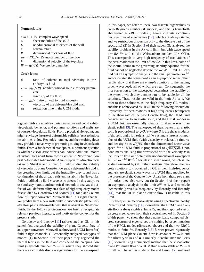
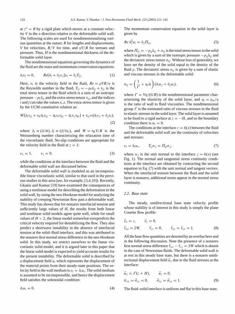
calculatec(0) using the symbolic packageMathematica. Re-sults from our calculations show that while the leading ordersolutions are purely real for HFGL modes in a rigid chan-nel, the leading order solutions forc(0) are complex whenthe wall is deformable. For small values ofΓ , the imaginarypart ofc(0) ispositive(system unstable) for downstream trav-eling waves (real part ofc(0) is positive), and the imaginarypart ofc(0) isnegativefor upstream traveling waves (real partof c(0) negative). Interestingly, the imaginary part ofc(0) fordownstream and upstream traveling waves has the same mag-nitude, but opposite signs; simply put, if the complex numberc(0) is written asa + ib (a, b positive) for downstream waves,then the result for upstream waves is given by−a − ib. Figs.4 and 5show the variation ofc(0)

i with Γ for the first twoHFGL modes, and this shows that the HFGL modes becomeunstable as the solid wall becomes deformable. AsΓ is in-c (0) ions.

A dd thes nt e up-s treamti alld thed

usi blew ,fl flowl ngb ughtt ta rder( lingb rninge s int uityc rmsi rderp htit inc s

erface, and this term was shown to be responsible foow-Re instability of Newtonian plane Couette flow by K

aran et al.[3], and by Shankar and Kumar[10] for vis-oelastic plane Couette flow in the creeping flow limit. Inresent low-Reasymptotic analysis, however, that particu

erm does not appear at leading order in the tangential veondition.

The leading order governing equations(35) and (51)cane analytically solved to give the following solutions forv

(0)z

ndu(0)z :

˜ (0)z = A1 exp[kz] + A2 exp[−kz]

+A3 exp[k(−iW +√

1 + W2 − (c(0))2W)z]

+A4 exp[−k(iW +√

1 + W2 − (c(0))2W)z], (56)

˜ (0)z = B1 exp[kz] + B2 exp[−kz] + B3 exp[γz]

+B4 exp[−γz], (57)

hereγ = k

√1 − Γ (c(0))2/(1 − ikc(0)η

(0)r Γ ), and the con

tants{A1 · · ·A4} and{B1 · · ·B4} must be determined frohe boundary and interface conditions. The above leadiner solutions are substituted in the interface conditions,52)–(55), as well as in the four boundary conditions atz = 1ndz = −H , and this system of equations is expressed in

rix form asAx = 0, whereA is an 8× 8 matrix containinghe eight conditions, andx is the vector of eight constanA1 · · ·B4}. The determinant of the matrixA is set to zero tbtain the characteristic equation.

reased,ci oscillates between stable and unstable reg

lso, the two curves inc(0)i versusΓ plots for upstream an

ownstream traveling waves differ only in sign, and haveame magnitude for all values ofΓ . In other words, whehe downstream traveling waves are unstable (stable), thtream traveling waves are stable (unstable). For downsraveling waves,Fig. 6shows thatc(0)

i ∝ Γ 2 for Γ � 1, i.e.n the limit very small solid deformability. Furthermore, weformability is found to have a destabilizing effect on alliscrete HFGL modes.

It is instructive to contrast this result with the previonstability of UCM plane Couette flow past a deformaall analyzed by Shankar and Kumar[10]. In their analysisuid and solid inertia were neglected in the creepingimit, and the instability was primarily driven by the couplietween the base flow and interfacial fluctuations thro

he tangential continuity condition (Eq.(23)). However, inhe present asymptotic analysis, the coupling termdoes noppear in the tangential velocity condition at leading osee Eq.(53)). In contrast, in the present case, the coupetween base flow and fluctuations occurs in the govequations due to the nonlinear upper-convected term

he UCM constitutive relation, and via the stress continonditions at the interface. Furthermore, the inertial ten the fluid and the solid medium appear in the leading oroblem despite theRe � 1 limit, in marked contrast wit

he earlier analysis of Shankar and Kumar[10]. Anothermportant difference is that in the earlier analysis of[10],he flow becomes unstable only ifΓ is greater than a certaritical value in theRe = 0 limit, and this critical value i


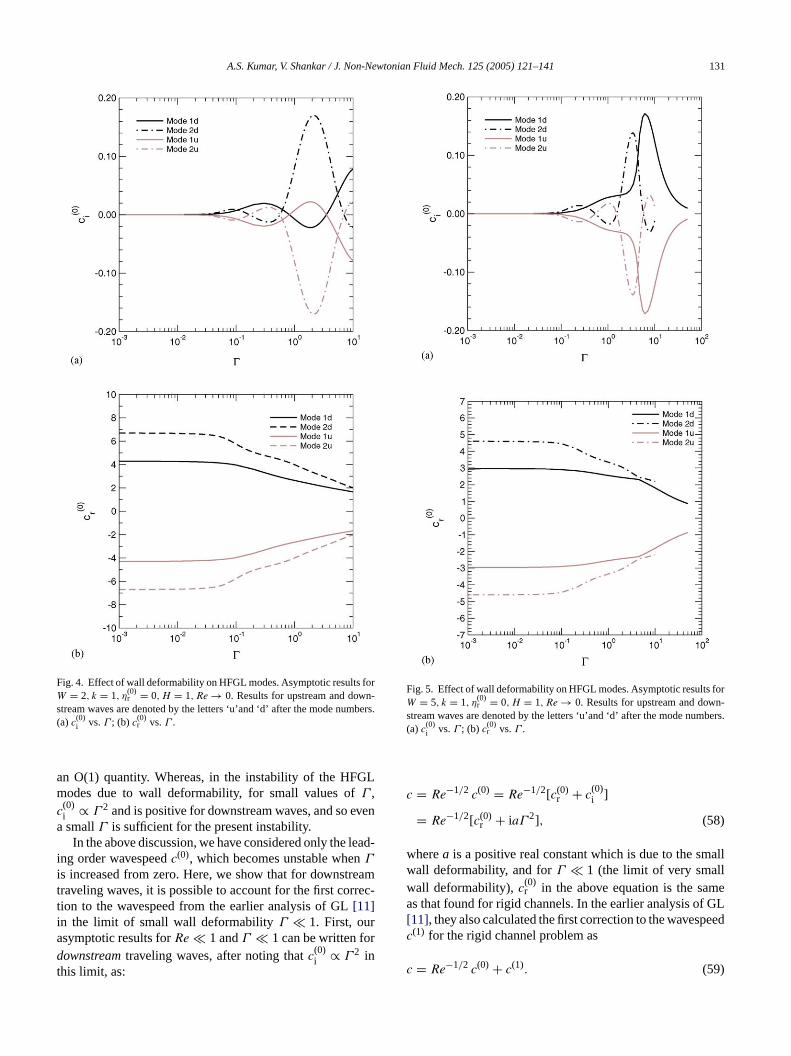
Fig. 4. Effect of wall deformability on HFGL modes. Asymptotic results forW = 2, k = 1, η(0)

r = 0, H = 1, Re → 0. Results for upstream and down-stream waves are denoted by the letters ‘u’and ‘d’ after the mode numbers.(a) c(0)

i vs.Γ ; (b) c(0)r vs.Γ .

an O(1) quantity. Whereas, in the instability of the HFGLmodes due to wall deformability, for small values ofΓ ,c

(0)i ∝ Γ 2 and is positive for downstream waves, and so even

a smallΓ is sufficient for the present instability.In the above discussion, we have considered only the lead-

ing order wavespeedc(0), which becomes unstable whenΓis increased from zero. Here, we show that for downstreamtraveling waves, it is possible to account for the first correc-tion to the wavespeed from the earlier analysis of GL[11]in the limit of small wall deformabilityΓ � 1. First, ourasymptotic results forRe � 1 andΓ � 1 can be written fordownstreamtraveling waves, after noting thatc(0)

i ∝ Γ 2 inthis limit, as:

Fig. 5. Effect of wall deformability on HFGL modes. Asymptotic results forW = 5, k = 1, η(0)

r = 0, H = 1, Re → 0. Results for upstream and down-stream waves are denoted by the letters ‘u’and ‘d’ after the mode numbers.(a) c(0)

i vs.Γ ; (b) c(0)r vs.Γ .

c = Re−1/2 c(0) = Re−1/2[c(0)r + c

(0)i ]

= Re−1/2[c(0)r + iaΓ 2], (58)

wherea is a positive real constant which is due to the smallwall deformability, and forΓ � 1 (the limit of very smallwall deformability),c(0)

r in the above equation is the sameas that found for rigid channels. In the earlier analysis of GL[11], they also calculated the first correction to the wavespeedc(1) for the rigid channel problem as

c = Re−1/2 c(0) + c(1). (59)


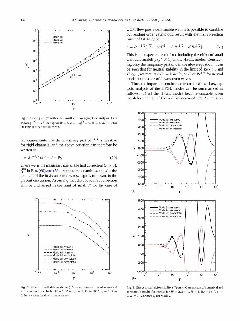
Fig. 6. Scaling ofc(0)i with Γ for smallΓ from asymptotic analysis. Data

showingc(0)i ∼ Γ 2 scaling forW = 5, k = 1, η(0)

r = 0, H = 1, Re → 0 forthe case of downstream waves.

GL demonstrate that the imaginary part ofc(1) is negativefor rigid channels, and the above equation can therefore bewritten as

c = Re−1/2 c(0)r + d − ib, (60)

where−b is the imaginary part of the first correction (b > 0),c

(0)r in Eqs.(60) and (58)are the same quantities, andd is the

real part of the first correction whose sign is irrelevant to thepresent discussion. Assuming that the above first correctionwill be unchanged in the limit of smallΓ for the case of

F ala0

UCM flow past a deformable wall, it is possible to combineour leading order asymptotic result with the first correctionresult of GL to give:

c = Re−1/2[c(0)r + iaΓ 2 − ibRe1/2 + d Re1/2]. (61)

This is the expected result forc including the effect of smallwall deformability (Γ � 1) on the HFGL modes. Consider-ing only the imaginary part ofc in the above equation, it canbe seen that for neutral stability in the limit ofRe � 1 andΓ � 1, we requireaΓ 2 = bRe1/2, orΓ ∝ Re1/4 for neutralmodes in the case of downstream waves.

Thus, the important conclusions from ourRe � 1 asymp-totic analysis of the HFGL modes can be summarized asfollows: (1) all the HFGL modes become unstable whenthe deformability of the wall is increased. (2) AsΓ is in-

Fig. 8. Effect of wall deformability (Γ ) onci : Comparison of numerical andasymptotic results for results forW = 2, k = 1, H = 1, Re = 10−4, ηr =0,Σ = 0. (a) Mode 1; (b) Mode 2.

ig. 7. Effect of wall deformability (Γ ) on cr : comparison of numericnd asymptotic results forW = 2, H = 1, k = 1, Re = 10−4, ηr = 0,Σ =. Data shown for downstream waves.


creased, thec(0)i versusΓ curves show oscillations between

stable and unstable regions, with the variation for down-stream traveling waves being completely antiphase with thatfor upstream traveling waves. Thus, when downstream trav-eling waves are unstable (stable), upstream traveling wavesare stable (unstable). (3) The imaginary part of the lead-ing order wavespeed for downstream waves is positive evenfor very small values ofΓ , andc(0)

i ∝ Γ 2 in this limit. (4)In the limit of smallRe, the viscosity ratioηr in the solidlayer should be O(Re1/2) for this instability to exist. (5)In the limit of small Re and Γ , it is argued (afterqual-itatively taking the first correction into account) thatΓ ∝Re1/4 for neutrally stable modes in the case of downstreamwaves.

4.1.1. Extension to Oldroyd-B fluidIt is useful here to examine the applicability of the above

asymptotic results to the Oldroyd-B fluid with nonzero sol-vent viscosity ratioβ. To this end, we substitute the scalingsintroduced in the foregoing discussion (Eqs.(34)–(40)) inthe linearized momentum equations for the Oldroyd-B fluid(Eqs.(29) and (30)). It can be readily verified that in orderfor the solvent viscous stresses in the momentum equationsto be of the same order as the polymer stresses and the inertialstresses in the Oldroyd-B fluid, it is necessary to stipulate thatβ ∼ Re1/2 � 1, implying the limit of zero solvent viscosityratio at very lowRe. For finiteβ, the solvent viscous stressesare O(Re−1/2) larger than the inertial stresses and the poly-mer stresses in the fluid; therefore, the polymer stresses and

Ff

ig. 9. Neutral stability curves in theΓ–Replane, forW = 1,H = 1,k = 1,ηr = 0or upstream and downstream waves are shown in gray and black curves re

,Σ = 0. ‘S’ and ‘U’ denote stable and unstable regions, and neutral curvesspectively. (a) Mode 1; (b) Mode 2; (c) Mode 3; (d) Mode 4.


Fig. 10. Neutral stability curves in theΓ–Replane, forW = 5, H = 1, k = 1, ηr = 0, Σ = 0. ‘S’ and ‘U’ denote stable and unstable regions, and neutralcurves for upstream and downstream waves are shown in gray and black curves respectively. (a) Mode 1; (b) Mode 2; (c) Mode 3; (d) Mode 4.

the inertial stresses do not appear at leading order, and onerecovers a Newtonian fluid. Because a Newtonian fluid doesnot admit elastic shear waves, there are no solutions toc atthis order. Consequently, the instability of the HFGL modesis not present for Oldroyd-B fluid at very lowRe for finitevalues of solvent viscosity ratio. This discussion thus sug-gests that the presence of solvent viscosity has a stabilizingeffect on the HFGL instability. However, at finiteRe ∼ O(1),it is not possible to neglect the polymer stresses and inertialstresses in the Oldroyd-B fluid, and it is possible that theHFGL mode instability of the UCM fluid continues to bepresent in the Oldroyd-B fluid with nonzero solvent viscos-ity ratio for finiteRe. This indeed turns out to be the case, aswe demonstrate numerically in Section4.2.2.

4.2. Results from numerical method

In this section, we examine the effect of wall deforma-bility on the HFGL modes at finiteReusing the numericalmethod described in Section2.4. We use the asymptoticresults from the previous section as starting guesses for thenumerical method. The asymptotic analysis of the previoussection gives rise to the following issues and questionswhich will be addressed using the numerical method: (1)The asymptotic results are valid in the limitRe � 1; will thisinstability persist at intermediate and highRe? (2) How doesthe finite-Recontinuation of the HFGL mode instability dueto wall deformability contrast with the finite-Recontinuationof the instability analyzed by Shankar and Kumar[10],


Fig. 11. Scaling ofΓ with Re for small Re: numerical data showingΓ ∼ Re1/4 scaling fork = 1, η(0)

r = 0, H = 1,Σ = 0, in agreement withasymptotic prediction for downstream waves.

who showed that the ZRGL mode becomes unstable inthe creeping flow limit when the wall is made sufficientlydeformable? (3) The low-Re asymptotic analysis in theprevious section requires that the solid–fluid viscosity ratioηr should scale asRe1/2 in theRe � 1 limit in order for theinstability to exist. What is the effect of increasingReon thisrestriction onηr ? Will the instability be present for finitevalues ofηr at finiteRe? (4) The previous analysis of Shankarand Kumar[10] also showed that the instability of the ZRGLmode due to wall deformability is essentially a continuationof the instability already present in Newtonian fluids[3],

F a-b ra

modified by the fluid viscoelastic effects. Will the presentinstability of the HFGL modes due to wall deformability bepresent in the limit of Newtonian fluids, i.e., forW � 1?

To answer the above questions, we now turn to the resultsfrom our numerical method.Figs. 7 and 8show the com-parison of the results obtained from the asymptotic analysisdescribed in the previous section with the numerical resultsobtained by solving the complete linear stability equations. Inthe plot ofci versusΓ in Fig. 8, it is clear that for downstreamwaves, the asymptotic result forci is positive in the limit ofΓ → 0, while the numerical (and exact) result forci is nega-tive up to a critical value ofΓ . The asymptotic prediction isalways positive in the limit of smallΓ because we have notcalculated the first correction to the wavespeed (which has

Fig. 13. Fluid velocity eigenfunction plots for ZRGL and HFGL modespast a deformable wall: data forW = 1,H = 1,k = 1. (a)Re = 10−4, Γ =9.93, cr = 0.253, ci = 0; ZRGL mode. (b)Re = 1, Γ = 1, cr = 6.64, ci =−0.54; HFGL mode.

ig. 12. Neutral stability curve in theΓ–Replane for the ZRGL mode destilized by wall deformability: continuation of the zero-Reresults of Shankand Kumar[10] to finite and largeRe.


a stabilizing effect) in the present analysis. This observationis also consistent with the prediction in Section4.1 that at agiven nonzeroRe, there exists a critical value ofΓ ∝ Re1/4

for downstream waves to be unstable. In the plots shownin Fig. 8, Re = 10−4, and so it takes a finite (but numeri-cally small) value ofΓ for the downstream waves to be un-stable. However, the asymptotic and numerical results agreevery well whenΓ ∼ O(1) for both downstream and upstreamwaves, because the stabilizing effect of the first correction di-minishes since it is O(Re1/2) smaller than the leading orderwavespeed. The agreement between asymptotic and numer-ical results forcr as a function ofΓ in Fig. 7 is also verygood.

In order to determine whether the predicted instability per-sists at finiteRe, neutral stability curves were computed in theΓ–Replane, for the first few HFGL modes and for a given set

of parametersW, k, ηr,Σ,H . These neutral curves are shownin Figs. 9–10. Let us first focus onFig. 9. We use the letter‘u’ after the mode number to indicate upstream waves, andthe letter ‘d’ after the mode number for downstream waves inthe following discussion and figures. InFig. 9, the unstableregions for all the modes extend only up to a small (but fi-nite)Re. Also, there are alternating regions in the parameterspace in which the downstream/upstream modes are stableor unstable. This is essentially a consequence of the oscilla-tory variation ofci with Γ shown inFig. 8. In these figures,W = 1, and the maximumReup to which the instability per-sists is around 0.1. However, whenW is increased to 5 inFig. 10, the nature of the neutral curves changes drastically.Fig. 10(a)shows the neutral curve for mode 1d (of the HFGLfamily) extends up to very highRe, andΓ ∝ Re−1 in thelimit of largeRe. However, mode 1u does not become unsta-

Fs

ig. 14. Neutral stability curves in theΓ–Wplane, forRe = 1,H = 1,k = 1,ηr =hown only for downstream waves. (a) Mode 1; (b) Mode 2; (c) Mode 3; (d) M

0,Σ = 0. ‘S’ and ‘U’ denote stable and unstable regions respectively. Dataode 4.


Fig. 15. Neutral stability curve in theΓ–W plane for the ZRGL modedestabilized by wall deformability: Data forRe = 1,H = 1, k = 1,ηr = 0,Σ = 0.

ble upon increasingΓ at anyRe. This can also be seen in thec

(0)i versusΓ curve from the asymptotic analysis shown in

Fig. 5(a). The other curves inFig. 10show that while thereexist alternating stable and unstable regions, the instabilitypersists up toRe ∼ 102. Data forW = 10 (not displayed inthis paper), along with the data presented here forW = 1and 5, confirm that theReup to which the instability per-sists increases with an increase inW. Fig. 11shows that forRe � 1,Γ ∼ Re1/4 for neutrally stable downstream waves,in agreement with the prediction of the asymptotic analysis ofSection4.1.

Fig. 12 shows the neutral curve in theΓ–Replane forthe continuation of the instability predicted in the creepingflow limit by Shankar and Kumar[10]. In that study, the au-thors showed that the ZRGL mode becomes unstable in theRe = 0 limit upon increasing wall deformability, and alsothat this unstable mode is essentially a continuation of the al-ready existent Newtonian fluid instability[3] to finiteW. Wecontinued theRe = 0 result of that paper to finiteRe, and theneutral curves inFig. 12for different values ofW show thatthe instability continues to highRe, and thatΓ ∼ Re−1/3 inthe limit of highRe. This scaling is similar to that reported forNewtonian plane Couette flow past a deformable wall at highReby Srivatsan and Kumaran[20]. However, these neutralcurves are qualitatively different from the neutral curves dis-cussed for the HFGL family of modes. In particular the highR -ts hisd lita-tsi heH red

to that required for the ZRGL mode, when the HFGL insta-bility exists. ForW = 5, the ZRGL mode is always stablefor the chosen value ofH = 1, and so this instability is ab-sent. However, the continuation of HFGL modes do becomeunstable forW = 5, as shown inFig. 10. Thus, these datashow that, at finiteW, the instability due to the continuationof the HFGL modes is a powerful mechanism compared tothe continuation of the ZRGL mode. It is instructive to con-sider the variation of the amplitude of perturbation velocities|vz| and|vx| with z, which further demonstrate the differencebetween the ZRGL and HFGL modes. This is displayed inFig. 13. While calculating these eigenfunctions, we fix theamplitude of the normal velocity component|vz| = 1 at thefluid–solid interfacez = 0. Fig. 13(a)shows the variationfor the ZRGL mode, whileFig. 13(b)shows the variationfor the HFGL mode, andW = 1 in both the cases. For theZRGL mode, the variation is monotonic fromz = 0 toz = 1,but the HFGL mode eigenfunctions exhibit oscillatory varia-tion. Oscillatory variation of the eigenfunctions is a signatureof the importance of elastic effects in HFGL modes, whilethe absence of this in the ZRGL modes indicates that fluidelasticity does not play an important role in the ZRGL insta-bility. This further suggests that the HFGL modes are absentin Newtonian fluids, and that the ZRGL mode instability issimilar to the instability of a Newtonian fluid flowing past adeformable wall.

heΓ Thed -sa ta-bi nd1 , ther -b nW es,a ilar.T ta allyd nt inN hisp

f Fort wt m-bd GLm s be-c ei olid,i db ilityo rfa-c s.

escalingΓ ∼ Re−1 shown inFig. 10(a)for the continuaion of the HFGL mode is very different from theΓ ∼ Re−1/3

caling obtained for the continuation of the ZRGL mode. Temonstrates that the two instabilities are driven by qua

ively different mechanisms. Comparing the data forW = 1hown for the two different instabilities inFigs. 9 and 12,t is clear that theΓ values required for destabilizing tFGL family of modes are typically very small compa

Figs. 14 and 15show the neutral stability curves in t–Wplane for both HFGL modes and the ZRGL mode.ata for the ZRGL mode (Fig. 15) clearly shows that the intability in the UCM fluid is a continuation to finiteWof thelready existent Newtonian fluid instability. Also, the insility exists only in a finite region of theΓ–W plane, and

s absent whenW increases beyond a critical value (aroufor the data shown in this figure). In marked contrast

esults for the HFGL mode (Fig. 14) show that the unstale region exists for finite and largeW, and is absent whe

→ 0. We show the data only for downstream modnd the data for upstream modes are qualitatively simhis comparison shows that theHFGL mode instability pasdeformable wall predicted in this study is fundamentue to the viscoelastic nature of the fluid, and is abseewtonian fluids. This is one of the central results of taper.

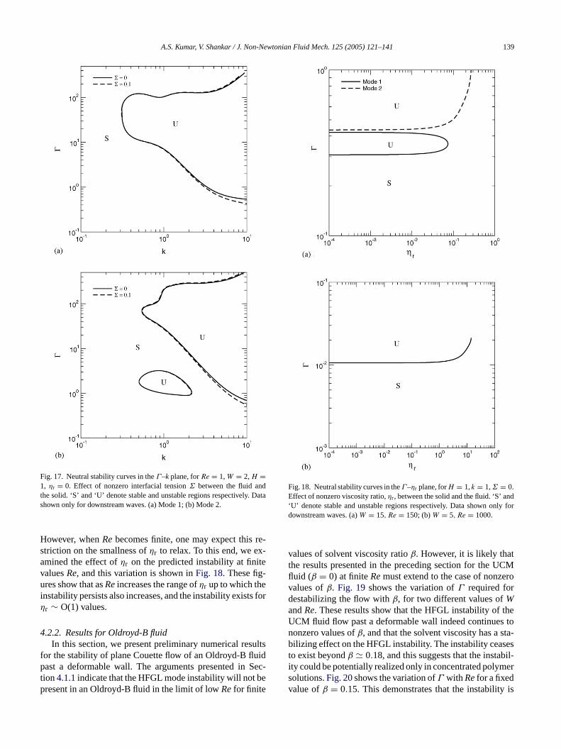
Fig. 16show the neutral stability curves in theΓ–k planeor both HFGL and ZRGL modes past a deformable wall.he case of HFGL modes (Fig. 16(a)–(c)), these results shohat the instability is absent in the limit of low wavenuers, but exists for finite and largek. In contrast,Fig. 16(d)isplays the neutral curve for the continuation of the ZRode which shows that only a finite band of wavenumber

ome unstable for this case.Fig. 17examines the effect of thnterfacial tension between the fluid and the deformable sn order to ascertain whether the large-kmodes are stabilizey nonzero interfacial tension. For the case of the instabf ZRGL modes due to the deformable wall, nonzero inteial tension has a stabilizing effect on large-kunstable mode


However, the results inFig. 17shows that the interfacial ten-sion does not stabilize the continuation of HFGL modes. Thissuggests that the destabilization of the HFGL modes by walldeformability is not an ‘interfacial instability’, and this re-sult is also in marked contrast with the continuation of theZRGL modes. It should be noted here that the UCM modelused here to describe the viscoelastic fluid does not haveany solvent contribution to the fluid stress, and the use ofan Oldroyd-B model has a stabilizing effect on these high-kunstable modes.

It is appropriate here to remark on the validity of the linearviscoelastic model used here to describe the deformation inthe solid. The base statex–directional strain in the solid wall(Eq. (9)) is proportional to the nondimensional quantityΓ ,and so strictly speaking the linear elastic solid model is validonly forΓ � 1. The study by Gkanis and Kumar[19] for the

case of Newtonian plane Couette flow past a neo-Hookeansolid (accounting for finite strains) showed however that forwall thicknessH > 2, the agreement between the linear andnonlinear solid models was very good even forΓ ∼ O(1).For the present class of modes, however,Γ ∼ 0.1 (or evensmaller) for destabilization by the deformable solid wall, andso the present predictions are expected to be accurate despitethe use of a simple linear viscoelastic model for the solid. Thedata presented for larger values ofΓ , however, may be modi-fied somewhat upon using a more complex model for the soliddeformation.

4.2.1. Results for nonzero solid viscosity ratioηrThe asymptotic analysis of Section4.1required thatηr ∼

O(Re1/2) in the limitRe � 1 in order for the elastic stressesin the solid to be as large as the viscous stresses in the solid.

Fs

ig. 16. Neutral stability curves in theΓ–kplane, forRe = 1,W = 2,H = 1,ηr =hown only for downstream waves for HFGL modes 1–3. (a) Mode 1; (b) Mo

0,Σ = 0. ‘S’ and ‘U’ denote stable and unstable regions respectively. Datade 2; (c) Mode 3; (d) ZRGL mode.


Fig. 17. Neutral stability curves in theΓ–kplane, forRe = 1,W = 2,H =1, ηr = 0. Effect of nonzero interfacial tensionΣ between the fluid andthe solid. ‘S’ and ‘U’ denote stable and unstable regions respectively. Datashown only for downstream waves. (a) Mode 1; (b) Mode 2.

However, whenRebecomes finite, one may expect this re-striction on the smallness ofηr to relax. To this end, we ex-amined the effect ofηr on the predicted instability at finitevaluesRe, and this variation is shown inFig. 18. These fig-ures show that asReincreases the range ofηr up to which theinstability persists also increases, and the instability exists forηr ∼ O(1) values.

4.2.2. Results for Oldroyd-B fluidIn this section, we present preliminary numerical results

for the stability of plane Couette flow of an Oldroyd-B fluidpast a deformable wall. The arguments presented in Sec-tion4.1.1indicate that the HFGL mode instability will not bepresent in an Oldroyd-B fluid in the limit of lowRefor finite

Fig. 18. Neutral stability curves in theΓ–ηr plane, forH = 1,k = 1,Σ = 0.Effect of nonzero viscosity ratio,ηr , between the solid and the fluid. ‘S’ and‘U’ denote stable and unstable regions respectively. Data shown only fordownstream waves. (a)W = 15, Re = 150; (b)W = 5, Re = 1000.

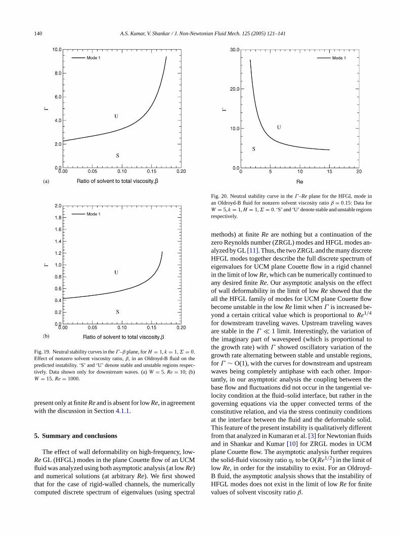
values of solvent viscosity ratioβ. However, it is likely thatthe results presented in the preceding section for the UCMfluid (β = 0) at finiteRemust extend to the case of nonzerovalues ofβ. Fig. 19 shows the variation ofΓ required fordestabilizing the flow withβ, for two different values ofWandRe. These results show that the HFGL instability of theUCM fluid flow past a deformable wall indeed continues tononzero values ofβ, and that the solvent viscosity has a sta-bilizing effect on the HFGL instability. The instability ceasesto exist beyondβ � 0.18, and this suggests that the instabil-ity could be potentially realized only in concentrated polymersolutions.Fig. 20shows the variation ofΓ withRefor a fixedvalue ofβ = 0.15. This demonstrates that the instability is


Fig. 19. Neutral stability curves in theΓ–β plane, forH = 1,k = 1,Σ = 0.Effect of nonzero solvent viscosity ratio,β, in an Oldroyd-B fluid on thepredicted instability. ‘S’ and ‘U’ denote stable and unstable regions respec-tively. Data shown only for downstream waves. (a)W = 5, Re = 10; (b)W = 15, Re = 1000.

present only at finiteReand is absent for lowRe, in agreementwith the discussion in Section4.1.1.

5. Summary and conclusions

The effect of wall deformability on high-frequency, low-ReGL (HFGL) modes in the plane Couette flow of an UCMfluid was analyzed using both asymptotic analysis (at lowRe)and numerical solutions (at arbitraryRe). We first showedthat for the case of rigid-walled channels, the numericallycomputed discrete spectrum of eigenvalues (using spectral

Fig. 20. Neutral stability curve in theΓ–Replane for the HFGL mode inan Oldroyd-B fluid for nonzero solvent viscosity ratioβ = 0.15: Data forW = 5,k = 1,H = 1,Σ = 0. ‘S’ and ‘U’ denote stable and unstable regionsrespectively.

methods) at finiteReare nothing but a continuation of thezero Reynolds number (ZRGL) modes and HFGL modes an-alyzed by GL[11]. Thus, the two ZRGL and the many discreteHFGL modes together describe the full discrete spectrum ofeigenvalues for UCM plane Couette flow in a rigid channelin the limit of lowRe, which can be numerically continued toany desired finiteRe. Our asymptotic analysis on the effectof wall deformability in the limit of lowReshowed that theall the HFGL family of modes for UCM plane Couette flowbecome unstable in the lowRelimit whenΓ is increased be-yond a certain critical value which is proportional toRe1/4

for downstream traveling waves. Upstream traveling wavesare stable in theΓ � 1 limit. Interestingly, the variation ofthe imaginary part of wavespeed (which is proportional tothe growth rate) withΓ showed oscillatory variation of thegrowth rate alternating between stable and unstable regions,for Γ ∼ O(1), with the curves for downstream and upstreamwaves being completely antiphase with each other. Impor-tantly, in our asymptotic analysis the coupling between thebase flow and fluctuations did not occur in the tangential ve-locity condition at the fluid–solid interface, but rather in thegoverning equations via the upper convected terms of theconstitutive relation, and via the stress continuity conditionsat the interface between the fluid and the deformable solid.This feature of the present instability is qualitatively differentfrom that analyzed in Kumaran et al.[3] for Newtonian fluidsap uirestl d-B y ofHv

nd in Shankar and Kumar[10] for ZRGL modes in UCMlane Couette flow. The asymptotic analysis further req

he solid-fluid viscosity ratioηr to be O(Re1/2) in the limit ofow Re, in order for the instability to exist. For an Oldroy

fluid, the asymptotic analysis shows that the instabilitFGL modes does not exist in the limit of lowRefor finitealues of solvent viscosity ratioβ.


The low-Reunstable modes were numerically continuedto finiteRe, and this showed that in most cases the instabilitypersists only up to a finiteRe, and theReup to which theinstability exists increases with an increase inW. However,in certain cases, the instability continues to largeRe, andΓ ∝ Re−1 in the limit Re 1. This is in marked contrastwith the continuation of the ZRGL mode instability past adeformable wall to highRe, which showed thatΓ ∝ Re−1/3

for this class of modes. Neutral curves constructed in theΓ–W plane showed that while the instability of ZRGL modedue to the deformable wall is essentially the continuation ofthe Newtonian fluid instability to finiteW, the HFGL modesexhibit the completely opposite behavior: the HFGL modeinstability exists only for finite and large values ofW, andis absent in the Newtonian fluid limit ofW → 0. Althoughour asymptotic analysis revealed that the HFGL mode in-stability requiresηr ∼ O(Re1/2) in the limit of low Re, nu-merical computation at finiteReshowed that the instabilitypersists forηr ∼ O(1) values. Neutral stability curves in theΓ–k plane further illustrate the difference between the effectof wall deformability on ZRGL modes and HFGL modes.While ZRGL modes are unstable only for a finite band ofwavenumbers in theΓ–k plane, HFGL modes are unstablefor intermediate and large wavenumbers, and they are stablefor small wavenumbers. The interfacial tension between thefluid and the deformable solid was shown to have negligiblee n-s sta-b ringi byt fort es est tioβ fF l-u ,t nsta-b fluidp thevfl

References

[1] M.A. Unger, H.-P. Chou, T. Thorsen, A. Scherer, S.R. Quake, Mono-lithic microfabricated valves and pumps by multilayer soft lithography,Science 288 (2000) 113–116.

[2] A. Groisman, S.R. Quake, A microfluidic rectifier: anisotripic flowresistance at low Reynolds number, Phys. Rev. Lett. 92 (2004) 094501.

[3] V. Kumaran, G.H. Fredrickson, P. Pincus, Flow induced instability ofthe interface between a fluid and a gel at low Reynolds number, J. Phys.II France 4 (1994) 893–904.

[4] V. Kumaran, Stability of the viscous flow of a fluid through a flexibletube, J. Fluid Mech. 294 (1995) 259–281.

[5] V. Kumaran, Stability of fluid flow through a flexible tube at interme-diate Reynolds number, J. Fluid Mech. 357 (1998) 123–140.

[6] V. Kumaran, Stability of wall modes in a flexible tube, J. Fluid Mech.362 (1998) 1–15.

[7] V. Shankar, V. Kumaran, Stability of non-parabolic flow in a flexibletube, J. Fluid Mech. 395 (1999) 211–236.

[8] V. Shankar, V. Kumaran, Stability of fluid flow in a flexible tube tonon-axisymmetric disturbances, J. Fluid Mech. 408 (2000) 291–314.

[9] V. Shankar, V. Kumaran, Stability of wall modes in fluid flow past aflexible surface, Phys. Fluids 14 (2002) 2324–2338.

[10] V. Shankar, S. Kumar, Instability of viscoelastic plane Couette flowpast a deformable wall, J. Non-Newtonian Fluid Mech. 116 (2004)371–393.

[11] V.A. Gorodtsov, A.I. Leonov, On a linear instability of plane parallelCouette flow of viscoelastic fluid, J. Appl. Math. Mech. 31 (1967)310–319.

[12] H.J. Wilson, M. Renardy, Y. Renardy, Structure of the spectrum in zeroReynolds number shear flow of the UCM and Oldroyd-B liquids, J.

[ New

[ f an22

[ anech.

[ astic, J.

[ ly

[ ions,

[ neo-

[ and

ffect on the high-k HFGL modes, and this further demotrates that the present instability is not an ‘interfacial inility’, rather it occurs due to dynamical processes occur

n the bulk of the viscoelastic fluid which are modifiedhe deformable solid layer. Preliminary numerical resultshe Oldroyd-B model were presented at finiteRe, and theshowed that the HFGL instability of the UCM fluid continuo be present in an Oldroyd-B fluid for solvent viscosity ra� 0.2, and the instability is absent for higher values oβ.or a fixed value ofβ, the instability exists only at finite vaes ofReand is absent in the limit of lowRe. In conclusion

he present study theoretically predicts a new class of ule modes in the plane Couette flow of a viscoelasticast a deformable solid wall which arise primarily due toiscoelastic nature of the fluid, and areabsentin Newtonianuids.

Non-Newtonian Fluid Mech. 80 (1999) 251–268.13] L. Landau, E. Lifshitz, Theory of Elasticity, Pergamon Press,

York, 1989.14] M. Renardy, Y. Renardy, Linear stability of plane Couette flow o

upper convected Maxwell fluid, J. Non-Newtonian Fluid Mech.(1986) 23–33.

15] M. Renardy, A rigorous stability proof for plane Couette flow ofupper convected Maxwell fluid at zero Reynolds number, Eur. J. MB: Fluids 11 (1992) 511–516.

16] R. Sureshkumar, A.N. Beris, Linear stability analysis of viscoelPoiseuille flow using an Arnoldi based orthogonalization algorithmNon-Newtonian Fluid Mech. 56 (1995) 151–182.

17] T.C. Ho, M.M. Denn, Stability of plane Poiseuille flow of a highelastic liquid, J. Non-Newtonian Fluid Mech. 3 (1977) 179–195.

18] R.G. Larson, Constitutive Equations for Polymer Melts and SolutButterworths, Boston, 1988.

19] V. Gkanis, S. Kumar, Instability of creeping Couette flow past aHookean solid, Phys. Fluids. 15 (2003) 2864–2871.

20] L. Srivatsan, V. Kumaran, Stability of the interface between a fluidgel, J. Phys. II. France 7 (1997) 947–963.

Instability of high-frequency modes in viscoelastic plane Couette...

Documents

Transcript of Instability of high-frequency modes in viscoelastic plane Couette...