Insights from a pseudospectral approach to the … from a pseudospectral approach to the Elder...

Insights from a pseudospectral approach

to the Elder problem

Maarten van Reeuwijk,1 Simon A. Mathias,1 Craig T. Simmons,2 and James D. Ward2

Received 3 September 2008; revised 23 January 2009; accepted 9 February 2009; published 17 April 2009.

[1] The aim of this paper is to clarify and circumvent the issue of multiple steady statesolutions in the Elder problem. A pseudospectral method is used to avoid numerical errorassociated with spatial discretization. The pseudospectral method is verified bycomparison to an analytical solution at Rayleigh number, Ra = 0, and by reproducing thethree stable steady state solutions that are known to exist at Ra = 400. A bifurcationdiagram for 0 < Ra < 400, which is free of discretization error, confirms that multiplesteady states are indeed an intrinsic characteristic of the Elder problem. The existence ofmultiple steady states makes the Ra = 400 Elder problem less suitable for benchmarkingnumerical models. To avoid the multiple steady states, we propose a benchmark atRa = 60. The results for this Low Rayleigh Number Elder Problem are presented andcompared to simulations with the commercial groundwater modeling package FEFLOW.Correspondence between the pseudospectral model and FEFLOW is excellent.

Citation: van Reeuwijk, M., S. A. Mathias, C. T. Simmons, and J. D. Ward (2009), Insights from a pseudospectral approach to the

Elder problem, Water Resour. Res., 45, W04416, doi:10.1029/2008WR007421.

1. Introduction

[2] The simulation of buoyancy driven flow (BDF) isfrequently required in many areas of hydrology includingsaline contamination [Zimmermann et al., 2006; Bolster etal., 2007; Narayan et al., 2007; Lin et al., 2009] and morerecently carbon sequestration [Riaz et al., 2006; Farajzadehet al., 2007; Hassanzadeh et al., 2007]. A major issue inBDF modeling is the problem of benchmarking [Simpsonand Clement, 2003; Simmons, 2005; Goswami and Clement,2007]. Typically, numerical models are verified by compar-ison with analytical solutions. Because of the nonlinearnature of BDF, analytical solutions often assume the exis-tence of a sharp interface between heavy and light fluids[e.g., Bear and Dagan, 1964; Huppert and Woods, 1995;Kacimov and Obnosov, 2001] and are therefore unable totest a numerical model’s ability to simulate buoyancy drivenconvective mixing. Park [1996] managed to relax this sharpinterface assumption but at the expense of being restrictedto one-dimensional flow only. More recently, Dentz et al.[2006] improved on this by deriving a perturbation-basedanalytical solution to the two-dimensional steady stateproblem of Henry [1964] [see also Simpson and Clement,2004]. However, Henry’s problem is also consideredunsuitable in this context because the internal flow regimeis driven by the hydraulic boundary conditions as opposedto buoyancy forces associated with variable density [Simpsonand Clement, 2003]. Consequently, a popular method forbenchmarking BDF models is to compare against publishedresults from numerical solutions of the Elder [1967] prob-

lem [e.g., Voss and Souza, 1987; Simpson and Clement,2003; Soto Meca et al., 2007].[3] The Elder [1967] problem originates from a heat

convection experiment whereby a rectangular Hele-Shawcell was heated over the central half of its base. A quarter ofthe way through the experiment, Elder [1967] observed sixplumes, with four narrow plumes in the center and twolarger plumes at the edges. As the experiment progressed,only four plumes remained. Elder [1967] also presentedresults from an equivalent but simplified numerical model.In contrast to the experiment, the model exhibited thedevelopment of a single plume only. These numericalresults were subsequently reproduced by Voss and Souza[1987] using the USGS finite element code, SUTRA. Theproblem is that since then, there have been a significantnumber of published Elder problem simulations whichdramatically vary in the way the plumes develop and thenumber of plumes that remain once the system has reachedsteady state [Oldenburg and Pruess, 1995; Kolditz et al.,1997; Ackerer et al., 1999; Boufadel et al., 1999; Olteanand Bues, 2001; Frolkovic and de Schepper, 2000; Dierschand Kolditz, 2002]. These discrepancies have been attrib-uted to various issues including mesh resolution, variationin numerical schemes and the use of different formulationsfor the governing equations [Diersch and Kolditz, 2002;Woods et al., 2003; Woods and Carey, 2007; Park and Aral,2007; Al-Maktoumi et al., 2007]. More pertinently, using abifurcation analysis based on a finite volume model,Johannsen [2003] demonstrated a consistent existence ofthree stable and a further eight unstable steady state sol-utions, significantly questioning the sensibility of using theElder problem for benchmarking purposes.[4] The aim of this paper is to provide a reproducible and

accurate benchmark for the Elder problem, which does notsuffer from the ambiguities mentioned above. To providethe most accurate numerical solution possible, we use a

1Department of Civil and Environmental Engineering, Imperial CollegeLondon, London, UK.

2School of Chemistry, Physics and Earth Sciences, Flinders University,Adelaide, South Australia, Australia.

Copyright 2009 by the American Geophysical Union.0043-1397/09/2008WR007421

W04416

WATER RESOURCES RESEARCH, VOL. 45, W04416, doi:10.1029/2008WR007421, 2009

1 of 13

pseudospectral method based on sine and cosine seriesexpansions in the horizontal direction and a Chebyshevexpansion in the vertical. Pseudospectral methods are widelyused in the study of transitional and turbulent flows [e.g.,Hussaini and Zang, 1987], as they do not suffer from anynumerical errors, except for the error associated with trun-cating the infinite series [Boyd, 2001; Fornberg, 1996].Wooding [2007] provided a new analysis of the Salt LakeProblem [Simmons et al., 1999; Wooding et al., 1997] andsuggested the future use of spectral methods in the solutionof the transport equations used in simulating unstablevariable density flows. The Salt Lake Problem is a test casewhich has been the subject of a very similar discussion to theElder problem in terms of the current challenges faced byvarious numerical codes to accurately simulate BDF.[5] The pseudospectral method is verified by comparing

it to a new analytical solution of the purely diffusiveRayleigh Number Ra = 0 case, and by reproducing thethree stable steady state solutions at Ra = 400. The resultingmodel is used to revisit the bifurcation analysis ofJohannsen [2003] to gain insights into how the Elderproblem can be improved as a benchmarking tool. Theoriginal Elder problem benchmark is at Ra = 400, which hasmultiple steady states. We propose a low Rayleigh numberbenchmark test case at a reduced Ra = 60 where only onesteady state solution exists.

2. Governing Equations

[6] The governing equations, in dimensionless form,using the stream function formulation are (adapted fromHolzbecher [1998] and Al-Maktoumi et al. [2007])

@c

@tþ Ra

@y@z

@c

@x� @y

@x

@c

@z

� �¼ @2c

@x2þ @2c

@z2ð1Þ

@2y@x2

þ @2y@z2

¼ @c

@xð2Þ

Here, (1) is the prognostic equation for the concentrationc [-], and (2) is the diagnostic equation governing the streamfunction y [-]. Furthermore,

x ¼ x0

H; z ¼ z0

H; t ¼ DEt

0

fH2; c ¼ c0 � c0

c1 � c0ð3Þ

and Ra [-] is the Rayleigh number found from

Ra ¼ ar0kg c1 � c0ð ÞHmDE

; ð4Þ

where x0 [L] is horizontal distance, z0 [L] is vertical distance,t0 [T] is time, H [L] is the vertical extent of the system, f [-]is porosity, DE [L2T�1] is the effective diffusion coefficient,

c0 [ML�3] is solute concentration, c0 [ML�3] is the

freshwater solute concentration, c1 [ML�3] is the saltierwater solute concentration, k [L2] is permeability, g [LT�2]is gravitational acceleration, m [ML�1T�1] is dynamic

viscosity and a [M�1L3] and r0 [ML�3] define the

relationship between fluid density, r [ML�3] and solute

concentration c0, given by

r ¼ r0 1þ a c0 � c0ð Þð Þ ð5Þ

[7] The domain and boundary conditions for the Elderproblem are illustrated in Figure 1. As the governingequations and boundary conditions are symmetric, it suffi-ces to consider the right-half plane [0, 2] � [0, 1], for whichthe boundary conditions are

y ¼ 0; 0 � x � 2; 0 � z � 1; t ¼ 0

y ¼ 0; 0 � x � 2; z ¼ 0; t > 0

y ¼ 0; 0 � x � 2; z ¼ 1; t > 0

y ¼ 0; x ¼ 0; 0 � z � 1; t > 0

y ¼ 0; x ¼ 2; 0 � z � 1; t > 0 ð6Þ

c ¼ 0; 0 � x � 2; 0 � z � 1; t ¼ 0

c ¼ 0; 0 � x � 2; z ¼ 0; t > 0

c ¼ f xð Þ; 0 � x � 2; z ¼ 1; t > 0

@c

@x¼ 0; x ¼ 0; 0 � z � 1; t > 0

@c

@x¼ 0; x ¼ 2; 0 � z � 1; t > 0 ð7Þ

f xð Þ ¼ 1; 0 � x � 1

0; 1 < x � 2

�ð8Þ

3. Numerical Procedure

[8] The first step is to expand y and c in the horizontaldirection such that

y x; z; tð Þ ¼XMm¼1

ym z; tð Þ sin kmxð Þ ð9Þ

c x; z; tð Þ ¼XMm¼0

cm z; tð Þ cos kmxð Þ ð10Þ

where km = mp/2. The choice of sin and cos for y and crelates to their horizontal boundary conditions (recallDirichlet and Neumann respectively).

Figure 1. Schematic diagram of the problem geometry.

2 of 13

W04416 VAN REEUWIJK ET AL.: PSEUDOSPECTRAL APPROACH TO THE ELDER PROBLEM W04416

[9] We now invoke the horizontal and vertical dimen-sionless Darcy fluxes

qx ¼@y@z

; qz ¼ � @y@x

ð11Þ

such that equation (1) can be rewritten as

@c

@tþ Ra

@

@xqxcð Þ þ @

@zqzcð Þ

� �¼ @2c

@x2þ @2c

@z2ð12Þ

[10] From equations (9) and (11) it can be seen that qxwill be odd in x whereas qz will be even. Therefore,corresponding expansions for the products qxc and qzcshould be written as

qxc x; z; tð Þ ¼XMm¼1

cqxcm z; tð Þ sin kmxð Þ ð13Þ

qzc x; z; tð Þ ¼XMm¼0

cqzcm z; tð Þ cos kmxð Þ ð14Þ

[11] Substituting equations (9), (10), (13) and (14) intoequations (2) and (12) and using orthogonality of basisfunctions then leads to

@cm@t

þ Ra kmcqxcþ @cqzcm@z

� �¼ �k2mcm þ @2cm

@z2ð15Þ

and

�k2mym þ d2ym

dz2¼ �kmcm ð16Þ

Note that this transformation, once cqxcm and cqzcm have beendetermined, has decoupled equations (1) and (2) in thex direction, so that eachmodem can be solved independentlyof the other modes.[12] To numerically evaluate the above problem the first

step is to approximate the cosine and sine transforms andcorresponding inverses with their discrete counterparts. Wechoose to use DCT-I and DST-I, and their correspondinginverses, IDCT-I and IDST-I, which can be efficientlyimplemented using Fast Fourier transforms (FFT) [seeMartucci, 1994]. In this way it can be said that

ym z; tð Þ ¼ DST-I y xm; z; tð Þ½ ;

cm z; tð Þ ¼ DCT-I c xm; z; tð Þ½ ;

cqxcm z; tð Þ ¼ DST-I qxc xm; z; tð Þ½ ;

cqzcm z; tð Þ ¼ DCT-I qzc xm; z; tð Þ½ ;

qz xm; z; tð Þ ¼ IDCT-I �kmym z; tð Þh i

;

where

xm ¼ 2m

M; m ¼ 0; 1 . . .M ð17Þ

It should be noted that the DCT-I and DST-I methodscorrespond to cosine and sine transforms up to a prefactor[Martucci, 1994]. These prefactors should be applied beforethere is full correspondence.[13] In the z direction, the nonperiodicity of the boundary

conditions suggests the use of an expansion in Chebyshevpolynomials, Tk [Boyd, 2001, p. 10]:

p xð Þ ¼XNk¼0

~pkTk xð Þ ð18Þ

where [Boyd, 2001, p. 497]

T0 xð Þ ¼ 1; T1 xð Þ ¼ x; Tkþ1 xð Þ ¼ 2xTk xð Þ � Tk�1 xð Þ ð19Þ

The Chebyshev polynomials form a basis on the interval�1 � x � 1 which can be mapped to z using thetransformation x = 2z � 1. In physical space, the variablesare defined at the points

zn ¼xn þ 1

2; xn ¼ cos

npN

� ; n ¼ 0; 1 . . .N ð20Þ

where xn are known as the Chebyshev-Gauss-Lobattopoints. With this choice of collocation points, the nodalvalues of p(xn) and the Chebyshev coefficients ~pk are relatedby a discrete cosine transform (See Appendix A). Thestrong clustering of points near the top and bottom wall isadvantageous because of the large near-wall gradients in theElder problem.[14] The relationship of the Chebyshev coefficients of p

in (18) and its first derivative

dp

dx¼

XNk¼0

~p1ð Þk Tk xð Þ: ð21Þ

is given by

~p1ð Þ0

~p1ð Þ1

..

.

~p1ð ÞN�1

~p1ð ÞN

26666664

37777775 ¼ Dx

~p0~p1

..

.

~pN�1

~pN

2666664

3777775 ð22Þ

where Dx is a N + 1 � N + 1 sparse upper diagonaldifferentiation matrix given by (see Appendix A)

Dx ¼

0 1 0 3 0 5 . . . N

0 0 4 0 8 0 . . . 0

..

. . ..

6 0 10 . . . 2N

..

. . .. . .

. . .. . .

.

..

. . .. . .

. . ..

2N

..

. . .. . .

.0

..

. . ..

2N

0 . . . . . . . . . . . . 0

266666666666664

377777777777775

ð23Þ

W04416 VAN REEUWIJK ET AL.: PSEUDOSPECTRAL APPROACH TO THE ELDER PROBLEM

3 of 13

W04416

Note that the last row of Dx contains zeros only. This issignificant for enforcing the boundary conditions for ODEswith the so-called tau method.[15] The coefficients for the fully expanded (in both x

and z) functions of c, y, qx c and qzc are denoted by ~cm,n,~ym,n, ~ax;m,n and ~az;m,n, respectively. With a point distributionaccording to equation (20), these coefficients can beobtained using the discrete cosine transform DCT-I (seeAppendix A)

~ym;n tð Þ ¼ DCT-I ym zn; tð Þh i

~cm;n tð Þ ¼ DCT-I cm zn; tð Þ½

~ax;m;n tð Þ ¼ DCT-I cqxcm zn; tð Þ½

~az;m;n tð Þ ¼ DCT-I cqzcm zn; tð Þ½

In the expressions above, the prefactors have been omitted[see Martucci, 1994].[16] As discussed before, each mode m can be solved

independently of the other modes. Therefore, when thesecoefficients are grouped per mode m in the vectors ~cm =[~cm,0. . .~cm,N]

T, ~ym = [~ym,0. . .~ym,N]T, ~ax;m = [~ax;m,0. . .~ax;m,N]

T

and ~az;m = [~az;m,0. . .~az;m,N]T, the resulting system of

equations can be compactly written as

d~cmdt

¼ �Ra km~ax;m þ Dz~az;m� �

þ Dzz � k2mI� �

~cm; ð24Þ

and

Dzz � k2mI� �

~ym ¼ �km~cm ð25Þ

where I is the identity matrix, and Dz and Dzz are the first-and second-order differentiation matrices with respect to z,respectively. These matrices are connected to Dx in (23) bya simple coordinate transform: Dz = Dxdx/dz and Dzz =Dx2(dx/dz)2 (see Appendix A). In our case, dx/dz = 2.[17] The model solves for ~cm,n by time integrating (24).

Using equation (25), the coefficients ~ym,n can immediatelybe expressed in terms of ~cm,n through the inverse of thediscrete differential operator. At each time step, thecoefficients of the nonlinear terms ~ax;m,n and ~az;m,n need tobe recomputed. This is done by mapping ~ym,n and ~cm,n tophysical space, calculating the products qxc and qzc, andconverting back to the functional space. As discussed, themapping between the physical and functional space isachieved using discrete sine and cosine transforms. The

boundary conditions are enforced via the tau method, andare discussed in more detail in Appendix A.[18] For transient simulations, time integration can be

accurately achieved using the stiff integrator ODE15Savailable in any standard version of MATLAB [Shampineand Reichelt, 1997; Shampine et al., 1999]. AlthoughODE15S is used for the smaller simulations, the methodbecomes prohibitively expensive when M and N becomelarge. This is caused in particular by the strong clusteringtoward the walls in the z direction, which makes theeigenvalues of the discrete diffusion operator very large;consequently, extremely small time steps will be required.Therefore, a more efficient approach is to use an implicit-explicit procedure to obtain the highly resolved steady statesolutions of sections 4 and 5, where diffusion is discretizedby an Euler backward scheme, and advection by an Eulerforward scheme. This standard operator-splitting procedureis unconditionally stable for the diffusion, so that physicallymore relevant time steps can be used. Note that the first-order accuracy of the Euler scheme is no concession to thespectral accuracy of the method, when this scheme is usedto find steady state solutions.[19] Spectral methods can produce accurate solutions

with relatively few modes, because of an exponentialconvergence to the exact solution. However, the solutionhas to be sufficiently smooth; when the solution is notsmooth, convergence can be much weaker, as Gibbs phe-nomena may prevent pointwise convergence near disconti-nuities [Trefethen, 2000, p. 15]. In the Elder problem, thereis a discontinuity in the boundary condition at the top wall,as given in (8). To have control over the sharpness of thetransition (and hence the local convergence), (8) is replacedby

f xð Þ ¼ 1

21� tanh

x� 1

d

� �� ð26Þ

Here, d represents a transition length: the larger d, thesmoother the transition. Clearly, as d ! 0, the originalboundary condition (8) is recovered (see also Figure 2). Theinfluence of d on the solutions of the Elder problem isdiscussed in Appendix B. A useful byproduct of replacingequation (8) by (26) is that grid-independent solutions exist:sufficiently close to a discontinuity at the top wall, anumerical solution will never converge because the localgradients become steeper each time the grid is refined. Onemight even question the physical relevance of equation (8)in itself, as the discontinuity locally induces infinite fluxes,which cannot exist in reality.

4. Verification

[20] The pseudospectral code is verified in two ways: bya comparison to an analytical solution at Ra = 0 and to thethree stable steady state solutions at Ra = 400, as identifiedby Johannsen [2003]. The analytical solution to equations(1)–(7) at Ra = 0 is derived in Appendix C using a cosinetransform in the x direction and a Laplace transform for t.The solution is given by

c x; z; sð Þ ¼sinh s1=2z

� �2s sinh s1=2ð Þ

þX1m¼1

sin gmð Þ sinh lmzð Þ cos gmxð Þsgm sinh lmð Þ :

ð27Þ

Figure 2. Smoothed boundary condition at z = 1.

4 of 13


Here, s is the Laplace variable such that c(s) =R10

c(t)e�stdt.Equation (27) can be inverted numerically using the Stehfest[1970] algorithm [see also Valko and Abate, 2004].[21] The analytical solution at Ra = 0 at t = 0.03, 0.1, 0.3

and 1.0 is shown in Figures 7a–7d, respectively. Plotted inFigures 7a–7d are the solutions from the pseudospectralmethod for 97 � 33 modes. The value for d has been setto d = 0.005, which is too small a value for pointwiseconvergence very close to x = ±1. However, at thisresolution, the solution is globally converged, even at Ra =400, as will be demonstrated in the convergence studybelow. The overall accuracy is evident from the excellentagreement with the analytical solution in Figures 7a–7d.[22] Next, the three stable steady state simulations at

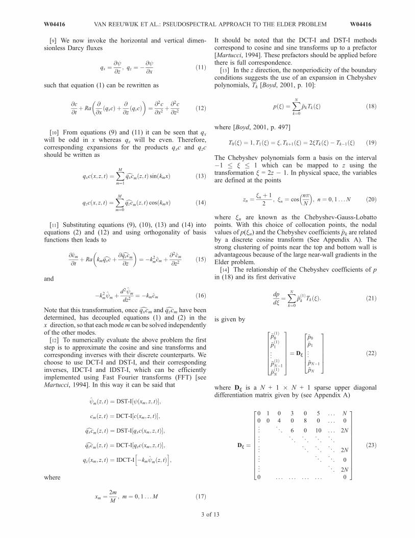
Ra = 400 (the original benchmark value for Ra), identifiedby Johannsen [2003], will be reproduced with thepseudospectral method. For this simulation, d is set to0.05, for which pointwise convergence is achieved at 513 �129 modes. This value of d is sufficiently small to capturethe important characteristics of the original Elder problem,as shown below and in Appendix B.[23] The three stable steady state solutions at Ra = 400

found with the pseudospectral method are shown inFigure 3. The steady state solutions are denoted by S1, S2and S3, where the subscript represents the number ofdownward plumes in the solution. Figure 3 shows theisolines of concentration with Dc = 0.1. The transientbehavior leading to the steady state are very similar to thosereported by Park and Aral [2007] and Woods and Carey[2007] and will not be shown here. For these simulations, asteady state was reached at t = 0.5 (which corresponds to200 convective time units when Ra = 400).[24] Steady state solutions S1 and S2 were found quite

easily, by using initial conditions of the form c(x, z, 0) =C (1 � (�1)mcos(pmx))/2 for 0 < x < 1, where m is an

integer. For x > 1, c(x, z, 0) = 0. By varying m and C,the simulation usually ends up either in S1 or S2.However, S3 cannot be found this way. In fact, we wereunable to independently obtain S3, despite trying a largeset of initial conditions (varying m, C, d, trying different zdependencies for c(x, z, 0), adding white noise). In the end,we digitized the concentration isolines of the S3 solution byJohannsen [2003]. The two-dimensional field for c was thenreconstructed by solving the system r2c = 0 with Gauss-Seidel iterations (a Laplace equation is a good inter-polator), subject to the boundary conditions and theinternal constraints imposed by the isolines. This resultedin an approximation of the S3 solution, which was thenused as an initial condition for the pseudospectral method.With this initial condition, the end result was indeed S3, aspresented in Figure 3c. Apparently, the basin of attractionof S3 is small; only a small subset of initial conditionsleads to S3.[25] A particularly good indicator for the system, as well

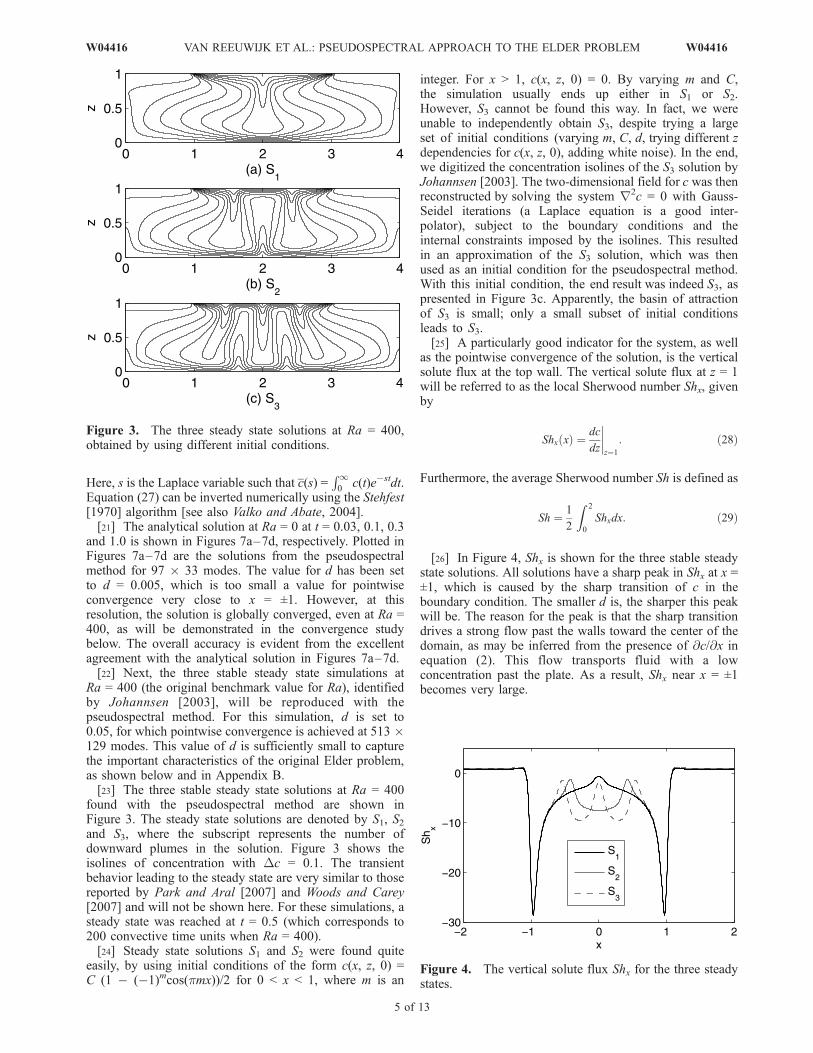
as the pointwise convergence of the solution, is the verticalsolute flux at the top wall. The vertical solute flux at z = 1will be referred to as the local Sherwood number Shx, givenby

Shx xð Þ ¼ dc

dz

��z¼1

: ð28Þ

Furthermore, the average Sherwood number Sh is defined as

Sh ¼ 1

2

Z 2

0

Shxdx: ð29Þ

[26] In Figure 4, Shx is shown for the three stable steadystate solutions. All solutions have a sharp peak in Shx at x =±1, which is caused by the sharp transition of c in theboundary condition. The smaller d is, the sharper this peakwill be. The reason for the peak is that the sharp transitiondrives a strong flow past the walls toward the center of thedomain, as may be inferred from the presence of @c/@x inequation (2). This flow transports fluid with a lowconcentration past the plate. As a result, Shx near x = ±1becomes very large.

Figure 4. The vertical solute flux Shx for the three steadystates.

Figure 3. The three steady state solutions at Ra = 400,obtained by using different initial conditions.


5 of 13

W04416

[27] At the location of a downward plume, Shx is reduced,while an upward plume causes an increase in Shx. As S1, S2and S3 differ in the number of the downward and upwardplumes, their Shx profile will differ in the number ofmaxima and minima. Consequently, Sh differs as well.Indeed, at Ra = 400, Sh is 3.5, 4.0 and 4.2 for solution S1, S2and S3, respectively. This distinguishing property will beused for the bifurcation diagram in section 5.[28] While pointwise convergence is reached at 513 �

129 modes for d = 0.05, global convergence, i.e.,convergence in a norm, is achieved much faster. Table 1lists the resolutions of ten simulations that have been usedfor a convergence study. The high-resolution solution S1(Figure 3a) has been used as the initial condition for allsimulations, and equations (24) and (25) were integratedwith the Euler implicit-explicit scheme until a steady statewas reached. Simulation 1 was the coarsest simulation thatconverged. The obtained steady state solutions of theconcentration field c(n) are compared to the concentrationfield c(ref) at the highest resolution (513 � 129), and theerror �(n) is calculated according to

� nð Þ ¼Rjc nð Þ � c refð ÞjdAR

dAð30Þ

[29] The fast convergence of the pseudospectral methodis evident in Figure 5. The error falls approximately with anexponent �6 up to a resolution of 97 � 33, where the erroris O(10�5). At higher resolutions, the convergence becomes

nonuniform, which is caused by the nonequidistant mappingin the z direction. When no interpolation is needed tocompare with the reference simulation (i.e., when Nz is 17,33, 65), the error relative to the fully resolved simulation islower.

5. Bifurcation Behavior

[30] Traditionally, the Elder problem has primarily beenused for benchmarking purposes. As a result, most studiesconsidered Ra = 400 only, and remarkably little was knownof the behavior of the solutions at lower Ra. Only recently,Johannsen [2003] used a finite volume code combined witha pseudo-arclength continuation method to construct abifurcation diagram of the Elder problem for 0 < Ra < 400.The study identified three stable solutions and an additionaleight unstable solutions, and showed that S2 and S3 (andtheir unstable counterparts) come into existence via a saddlenode (fold) bifurcation. In constructing a bifurcationdiagram, one has to characterize an entire solution by asingle number. Johannsen [2003] used a projection of thesolution which maximized the difference between thedifferent solution branches. In this study, the averageSherwood number Sh is used; as discussed in section 4,Sh is a good indicator to distinguish between S1, S2 and S3.[31] The bifurcation diagram (Figure 6) was obtained by

using each of the three steady state solutions S1, S2 and S3 atRa = 400 as initial conditions for a simulation at Ra = 390.This simulation was then run for 100 convective time units(which corresponds to t = 100/Ra diffusive time units) untilsteady state was reached. Sh was calculated, and the newsteady state solution was used as the initial condition Ra =380 and so on. Near the bifurcation points the Ra intervalswere reduced to 1 to capture the bifurcation properly. WhenS2 and S3 cease to exist at their respective bifurcation points,the flow solution converges to S1. The bifurcation points aredenoted by circles in Figure 6.[32] Figure 6 shows the bifurcation diagram for the Elder

problem for 0 < Ra < 400. The only solution which existsfor the entire range of Ra is S1. From Ra = 76 onwards, S2comes into existence via a fold bifurcation. Similarly, S3comes into existence at Ra = 172. An interesting detail isthat near the bifurcation points, Sh for S2 and S3 is lowerthan for S1. Sufficiently far away from the bifurcationpoints, solutions with more plumes have a higher Sh. The

Figure 5. Convergence behavior of the pseudospectralmethod.

Table 1. Resolutions Used for the Convergence Study of the

Pseudospectral Method

Simulation Nx Nz

1 25 132 29 153 33 174 65 255 97 336 129 417 193 498 257 659 385 9710 513 129

Figure 6. Bifurcation diagram of the Elder problem for0 < Ra < 400.

6 of 13


bifurcation points are comparable with Johannsen [2003],who reports that S2 and S3 come into existence at Ra = 67and Ra = 151, respectively. The slight differences are mostlikely caused by the different numerical methods.[33] It should be noted that there may be more than three

stable steady state solutions at Ra = 400. Indeed, thepseudo-arclength continuation method used by Johannsen[2003] provides a systematic way to follow the solutions asRa changes, but does not guarantee that all solutions arefound. Hence, it is imaginable that more than three stablesteady solutions exist. If they exist, these steady states willhave tiny basins of attraction, as they have not beenstumbled upon before.[34] For the Elder problem, the onset of convection as

characterized by the critical Rayleigh number Rac, is atRac = 0. This is clear from Figure 6, as Sh steadily increasesfrom Sh = 1/2 (the diffusive state) for Ra > 0. This behavioris different from the classical value of Rac = 4p2 for aninfinitely extending strip with constant boundary conditions[Horton and Rogers, 1945]. The difference in Rac originatesfrom the difference in boundary conditions. For the Elderproblem, the finite length of the c = 1 boundary conditiongenerates a concentration gradient @c/@x near x = ±1. Theexistence of a concentration gradient will drive a flow, as isevident in equation (2). As this gradient cannot be undoneby diffusive transport as is the case for the infinite strip,convection will occur for every Ra > 0.[35] Figure 6 clearly elicits the reason for the ambiguities

in using the Elder problem as a benchmark: at Ra = 400,three stable steady state solutions coexist. As a result, someregions of the space of initial conditions will converge to S1,other regions to S2 and yet others to S3. These regions maybe intertwined and even have fractal boundaries. Moreover,the governing equations, the numerics and the gridresolution will affect the shape and extent of these regions.Hence, the ambiguities with the Elder problem are physicalrather than numerical.[36] However, a pragmatic solution to the coexistence of

stable steady state solutions is also evident in Figure 6;simply lower Ra. Indeed, for Ra < 76, the Elder problem hasa single steady state solution. Hence, all initial conditionsshould converge to S1 for Ra < 76, so that the details of thegoverning equations, numerics and grid resolution becomemuch less crucial.

6. Low Rayleigh Number Elder Problem

[37] The original Elder problem is formulated for aRayleigh number of Ra = 400. We have seen that threesteady state solutions exist for the Elder problem: S1, S2 andS3. It has also been demonstrated that the Elder problem hasonly one steady state solution for Ra < 76. It is thereforeuseful to develop a test case version of the Elder problem atreduced Rayleigh number in the regime where only onesteady state solution exists. As we would like to besufficiently far from the bifurcation point, we choose Ra =60 as a new test case. We coin this new test case the LowRayleigh Number Elder Problem. At this Ra, all flowsolutions should converge to S1. Although the buoyancyforce at Ra = 60 is far less than at Ra = 400, transport byconvection remains significant. The Ra = 60 benchmark istherefore suitable for verification purposes. In addition, itcan be used to study the accuracy of the diffusive and

convective discretizations, as well as the time integrationscheme.[38] We compare results at Ra = 60 of the new

pseudospectral method with results from a standard variabledensity groundwater flow and solute transport model. Forthis purpose, FEFLOW version 5.3 [Diersch, 2005] wasused. Diersch [2005] provides exhaustive informationrelating to the FEFLOW variable density groundwater flowmodel. FEFLOW employs the fundamental physicalprinciples of fluid mass conservation, solute mass con-servation and momentum conservation. It has beensuccessfully tested on numerous benchmarks, includingthose reported for variable density flow, the details of whichare given by Diersch and Kolditz [2002] and Diersch[2005].[39] The standard Elder problem (high Rayleigh number

case of Ra = 400) was initially reproduced with FEFLOW.The details of this problem are reported in a vast body ofliterature and are not reproduced here. See Diersch andKolditz [2002, Table 1] for a complete listing of parametersused in the benchmark Elder problem case for Ra = 400 anda complete discussion on the results of the standard testcase. We modified this base case problem by adjusting theleft hand and right hand portions of the top boundaryadjacent to the solute source in order to be completelyconsistent with the boundary conditions used in thepseudospectral method (Figure 1). This involved changingthe top boundary condition to include a constant concentra-tion boundary of value c0 = c0 along the top boundary eitherside of the solute source (c0 = c1) present in the center of thetop boundary. Hence, the FEFLOW simulations uses theoriginal boundary condition (26), so that the transitionlength d is set implicitly by the horizontal mesh spacing atx = ±1. Note here that in the FEFLOW simulation wesimulate the full plane solution (total horizontal dimension =600 m) in order to ensure that the half plane solution usedelsewhere throughout this study is justifiable. There are wellknown examples in turbulence problems where governingequations and boundary conditions feature symmetries buttheir solutions do not. A simple example where thesymmetry breaks down is the problem of flow past a circularcylinder [Frisch, 1995]. Our results confirm that the halfplane solution and the full plane solution are entirelyconsistent. To lower the Rayleigh number of the system toRa = 60, the density contrast between the solute source andthe ambient initial fluid was reduced. This was achieved byreducing the concentration value of the upper solute sourceboundary (originally c0 = c1 = 1) to a new reduced value ofc0 = c1 = 60/400. Two grid discretizations are presentedhere: coarse utilizing 4,539 nodes (horizontal nodes = 89;vertical nodes = 51) and fine utilizing 17,877 nodes(horizontal nodes = 177; vertical nodes = 101). Asensitivity analysis to spatial discretization utilizing bothcoarser and finer grids ensured that the model resultspresented here were grid-independent and confirmed thatthe above spatial discretization was satisfactory. Timestepping in FEFLOW is regulated through the use of anautomatic time step increment. The choice of time step sizeis regulated by error checking (based on a Euclidean L2integral (RMS) error norm of 10�3) and the use of Couranttype stability criteria. Simulations were run in transientmode for 200 years simulated real time to reach a steady


7 of 13

W04416

state solution. The original Elder problem Ra = 400solutions are usually reported for timescales that are muchshorter, typically on the order of 20 years.[40] For the pseudospectral method, 97 � 33 modes were

employed, and the upper boundary condition (26) used avalue of d = 0.005. As for the Ra = 0 solution, this valueof d is too low to achieve pointwise convergence verynear the boundaries at x = ±1. However, as shown in theconvergence study, the solution has fully convergedglobally. Results comparing the pseudospectral methodand the FEFLOW simulations are shown in Figures 7e–7hfor dimensionless time t = 0.03, 0.1, 0.3, and 1. Thesecorrespond to real time values of 6, 20, 60 and 200 years,respectively, on the basis of scaling relations provided inequation (3). Results show excellent agreement between thepseudospectral method and the FEFLOW simulations withboth the fine and coarse grid resolutions. The coarse gridsimulation is slightly off in Figure 7g, but the fine grid

simulation has converged to the prediction of the pseudos-pectral method.

7. Concluding Remarks

[41] There has been much discussion in recent literatureabout the Elder Problem and the discrepancy betweenvarious numerical simulations in terms of the number ofconvection cells and the development of unstable plumes. Anumber of factors have been highlighted which appear toexplain, at least in part, the various discrepancies. Theseinclude different mesh resolutions, different formulations ofthe governing flow and transport equations, and differentnumerical solution schemes.[42] However, the underlying cause of these discrepan-

cies is not numerical but physical; at Ra = 400, there are atleast three stable steady state solutions, S1, S2, and S3, aswas shown in the bifurcation analysis of Johannsen [2003].This point has been largely ignored in the plethora of Elder

Figure 7 Isolines of the concentration field for t = 0.03, t = 0.1, t = 0.3 and t = 1.0 at Ra = 0 and Ra =60. (a)–(d) Comparison of the pseudospectral method (solid line) to the new analytical solution at Ra = 0(downward triangles). (e)–(h) Comparison of FEFLOW simulations with 89 � 51 (downward triangles)and 177 � 101 nodes (upward triangles) to the pseudospectral method (solid line).

8 of 13


problem benchmark studies. Because of the existence ofmultiple steady state solutions, the phase space will bepartitioned: some initial conditions will generate trajectorieswhich lead to S1, while others lead to S2 and yet others to S3.There may even be more than three stable solutions,although these have not yet been found. The basins ofattraction of S1, S2 and S3 are intertwined and may havefractal boundaries, so that slight variation of the initialconditions may lead to different steady states. It would beuseful for the Elder experiments to be repeated to checkwhether these different steady states can be reproduced inthe laboratory.[43] Differences in the governing equations, grid resolu-

tion and the employed discretization techniques will affectthe size and shape of the basins of attraction for the stablesolutions. Hence, even when using the same initial con-ditions, different codes may yield different steady states. Inthis study, we aimed to eliminate all sources of numericaldiscrepancy, in order to get uncontaminated insight into theambiguities associated with the Elder problem benchmark.For this reason, a pseudospectral method was employedwith sine and cosine series expansions in the horizontal, andChebyshev series expansions in the vertical. The key resultsof this study are as follows.[44] 1. The pseudospectral method has been successfully

used to simulate the Elder problem for a range of Rayleighnumbers including the original base test case at Ra = 400.[45] 2. Using the pseudospectral method, we find excel-

lent agreement with a new analytical solution for the purelydiffusive case at Ra = 0. We note that the critical Rayleighnumber for the Elder problem is Ra = 0, above which fluidmotion due to convection begins for any nonzero value ofthe unstable concentration difference.[46] 3. We have successfully used the pseudospectral

method to reproduce the three stable steady state solutionsat Ra = 400 reported previously by Johannsen [2003] in hisbifurcation analysis. Depending on the initial conditions,grid resolution, governing equations and discretization, thefinal solution to the Elder problem is seen to converge toone of three possible steady solutions S1, S2 and S3. Sincemultiple steady solutions exist to the Elder problem, thiscalls into question the usefulness of the Ra = 400 versionof the Elder problem as a model benchmark. Multiplesolutionsmake intercode comparisons cumbersome. Becauseof sensitive dependence of the flow evolution upon initialconditions, grid resolution, governing equations and dis-cretization, the flow solution may either be S1, S2 or S3. Atthe very least, it suggests that the original Ra = 400 Elderproblem benchmark should be used with caution and carefulinterpretation.[47] 4. Our bifurcation analysis shows that S1 exists for

0 < Ra < 400, while S2 and S3 exist for Ra � 76 and Ra �172, respectively. Hence, for Ra < 76, only a single steadystate solution exists. This suggests that an improved andreproducible benchmark test case would be one whoseRayleigh number is such that Ra < 76. We constructed a testcase for Ra = 60 in this lower Rayleigh number regime. Forthis new Low Rayleigh Number Elder Problem, results ofthe pseudospectral method were in excellent agreement withthose produced using a conventional variable densitygroundwater flow and solute transport simulator. Weprovide new solutions for the alternative test case Ra = 60

and propose this as a new benchmark test case which avoidsthe multiple steady state solutions that exist for cases whereRa > 76. In this regime, both convective flow (albeit ofreduced magnitude compared to Ra = 400 case) anddiffusion/dispersion control solute transport processes aresubstantial, and thus the relevant physical processes aretested.[48] It is noted that the original Elder problem with Ra =

400 can still be useful if taking into account the existence ofseveral steady state solutions. A complete benchmark testfor the Elder problem could consist of a series of Ra tests:(1) test Ra = 0 and compare to the given analytical solution,(2) test Ra = 60 and verify the unique steady state solutionand the transients leading to it, and (3) run the original Elderproblem at Ra = 400 and reproduce at least S1 and S2. Asimulation code which is able to satisfy all three tests couldbe considered as sufficiently verified for the Elder problem.[49] The use of pseudospectral methods appears promis-

ing in the solution of unstable free convective (gravitationalinstability) type problems. The absence of spatial discreti-zation errors makes pseudospectral methods a preferredchoice for studying convective instabilities. However, thesemethods will not be applicable to all instability problems, inparticular those with complex geometries and mixed typeboundary conditions. In these cases, finite volume, finiteelement or spectral element techniques are more suitable.Future studies should examine the wider applicability ofpseudospectral methods in a range of other free convectiontype problems.

Appendix A: Chebyshev Polynomials and theCosine Transform

[50] There is a wealth of information about spectralmethods available in the literature and in textbooks. Inparticular the application of collocation methods (whichare formulated in physical space and do not rely on FFTs)are well documented [Trefethen, 2000; Weideman andReddy, 2001; Fornberg, 1996]. However, the collocationmethods are limited to relatively few modes as thedifferentiation matrices are full; the computational require-ments scale as O(N2). In contrast, FFT-based Chebyshevmethods scale as O(N log N), which makes them thepreferred choice for large problems. However, an exactmethod to implement Chebyshev methods using FastFourier Transforms (FFT) was not readily outlined in asingle source. This appendix is intended as a very shortintroduction to using Chebyshev polynomials for differ-ential equations with the FFT.[51] At first sight the Chebyshev polynomials Tk in

equation (19) seem to have little to do with trigonometricfunctions. However, the formal definition of Tk is [Boyd,2001, p. 497]

Tk ¼ cos kqð Þ ðA1Þ

where q = arccos x. We can immediately see that (A1) isidentical to the first two terms of (19), as T0 = cos 0 = 1 andT1 = cos (arccos x) = x. The recursion rule Tk+1 = 2xTk� Tk-1can be obtained from substituting (A1) into the trigonometricidentity

2 cos q cos kq ¼ cos k þ 1ð Þqþ cos k � 1ð Þq: ðA2Þ


9 of 13

W04416

which immediately results in Tk+1 = 2 x Tk � Tk-1. Note that(A1) indicates that the Chebyshev polynomials are nothingmore than a cosine transform followed by a coordinatetransform according to q(x) = arccos x. Chebyshevpolynomials are orthogonal with respect to the weightingfunction 1/

ffiffiffiffiffiffiffiffiffiffiffiffiffi1� x2

p(which originates from the coordinate

transform):

Z 1

�1

TmTnffiffiffiffiffiffiffiffiffiffiffiffiffi1� x2

p dx ¼ p2cndmn; ðA3Þ

where dmn is the Kronecker delta, c0 = 2, and cn = 1 for all n >0. If the spacing of x is chosen according to the Chebyshev-Gauss-Lobatto points

xn ¼ cosnpN

� ; n ¼ 0; 1; . . . ;N ; ðA4Þ

then qn = arccos xn = np/N is equidistant. Therefore, theChebyshev expansion in equation (18) takes the form of adiscrete cosine transform [Boyd, 2001, p. 46] and can bewritten as

p xnð Þ ¼XNk¼0

~pk cos kqn: ðA5Þ

This property makes Chebyshev methods particularlyattractive from a computational perspective, as the transfor-mation from physical space to functional space can beefficiently carried out in O(N log N) operations using FFTs.[52] The Chebyshev coefficients ~pk in equation (18) are

related to the coefficients of the first derivative ~pk(1) of

equation (21) by a recurrence relation (in descending order)[Boyd, 2001, p. 177]

~p1ð ÞN�1 ¼ ~p

1ð ÞN ¼ 0

~p1ð Þk�1 ¼ 2k~pk þ ~p

1ð Þkþ1

2~p1ð Þ0 ¼ 2~p1 þ ~p

1ð Þ2

ðA6Þ

This recurrence relation can be derived using (A1) and atrigonometric identity [e.g., Johnson, 1996, p. 13]. From

(A6) it follows that the differentiation matrix Dx, defined inequation (22), is given by

Dx ¼

2 0 �1

0 1 . .. . .

.

. .. . .

. . ..

�1

. .. . .

.0

0 1

26666664

37777775

�10 2 0

. ..

4 . ..

. .. . .

.0

. ..

2N

0

26666664

37777775ðA7Þ

which results in (23) upon evaluation.[53] The use of Chebyshev methods in differential equa-

tions will be demonstrated using a Helmholtz equation,which resembles the equation for the stream function (16):

d2y

dx2þ y ¼ 2ex ðA8Þ

subject to y(0) = 1 and y(p/2) = 0. This differential equationhas the exact solution y = ex � ep/2 sin x. As the Chebyshevpolynomials are defined on �1 � x � 1, a change ofvariables as x = p(x + 1)/4 is used, which results in

16

p2

d2y

dx2þ y ¼ 2ep xþ1ð Þ=4 ðA9Þ

The Chebyshev polynomial coefficients for y, d2y/dx2 andr = 2ep (x+1)/4 will be denoted by ~yk, ~y

(2) and ~rk, respectively.Substituting the Chebyshev expansions into (A8), andinvoking orthogonality of the basis functions, we obtain

16

p2~y

2ð Þk þ ~yk ¼ ~rk : ðA10Þ

[54] As the vector ~y(2) = [~y0(2), . . ., ~yN

(2)]T is related to thevector ~y = [~y0, . . ., ~yN]

T by ~y(2) = Dx2 ~y, the resulting system

of equations is

L~y ¼ ~r; ðA11Þ

where L = 16p2 Dx

2 + I (note the correspondence to equation(25)).[55] The boundary conditions are enforced via the tau

method, i.e., by incorporating them in the last two rows ofL. This is permitted because the last two rows of Dx

2

ordinarily contain zeros only. Observing that Tk(x = �1) =(�1)k and Tk(x = 1) = 1, we set LN,k = (�1)k, LN+1,k = 1, RN =1, and RN+1 = 0. The Chebyshev solution can now bedetermined via ~y = L�1 ~r.[56] For further clarification concerning the relation

between the Chebyshev polynomials and the FFT, considerthe small code fragment which implements the solution of(A8) using Chebyshev polynomials in MATLAB, givenbelow. This fragment includes the construction of the dif-ferentiation matrix, the forward and inverse cosine trans-forms, applying the prefactors, the solution of the system,and the comparison with the analytical solution. The resultfor N = 5 polynomials is shown in Figure A1. Clearly, evenwith so few modes, the Chebyshev solution is practicallyindistinguishable from the analytical solution.

Figure A1. Solution of equation (8) with N = 5 Chebyshevpolynomials.

10 of 13


N = 5;%Set number of polynomials

xi = [cos(linspace(0, pi, N + 1))]’;

%Lobatto points

A = spdiags([[2;ones(N, 1)], -ones(N + 1, 1)],

[0 2], N + 1, N + 1);

B = spdiags([0;2*[1:N]’;0], 1, N + 1, N + 1);

Dxi = inv(A)*B;%Create differentiation matrix

x = (xi + 1)*pi/4; Dx = Dxi*4/pi;

%Transform to 0 < x < pi/2

L = Dx^2 + speye(N + 1, N + 1);%Form LHS

L(N, :) = (-1).^[0:N];L(N + 1, :)

= ones(1, N + 1);%Set BCs

r = 2*exp(x);%RHS of Helmholtz eqn.

rt = real(fft([r;r(N:-1:2)]));

rt = rt(1:N + 1);%DCT-I

rt = rt/N; rt([1 N + 1]) = rt([1 N + 1])/2;

%Prefactors

rt([N;N + 1]) = [1;0];%Set RHS of BCs

yt = inv(L)*rt;%Solve Helmholtz eqn

yt([1 N + 1]) = yt([1 N + 1])*2;%Prefactors

y = real(fft([yt;yt(N:-1:2)]));

y = y(1:N + 1)/2; %IDCT-I

xx = linspace(0, pi/2, 100);

f = exp(xx) - exp(pi/2)*sin(xx);%Analytical sol.

plot(x, y, ‘ks’,xx, f, ‘k-’);

legend(‘Cheb.’, ‘An.’);

Appendix B: Influence of d

[57] It may be questioned what the effect is of varying din equation (26) on the transients and the steady statesolutions of the Elder problem. We find that the transientsare very sensitive to d [see alsoWoods and Carey, 2007]. Asthe transients ultimately determine the final steady state, dinfluences whether the system will end up in S1, S2 or S3.However, once a steady state solution is obtained, varying donly changes the solution near the transition. Indeed, allthree steady state solutions at Ra = 400 are stable for d =0.05, d = 0.10, and d = 0.20, which represent sharp to rathersmooth transitions (see also Figure 2). The bifurcationpoints have a small dependence on d; for larger d, S2 and S3come into existence at slightly higher Ra.[58] Below we study the effect of d on the local

Sherwood number Shx. In Table B1, resolutions are givenfor simulations with d = 0.05, d = 0.10 and d = 0.20. The

resolution for each simulation is chosen such that thesolutions are pointwise converged. From Table B1 it is clearthat as d becomes smaller, the required resolution forpointwise convergence quickly increases: halving d requiresdoubling of the resolution.[59] Shown in Figure B1 is Shx as defined in (28) as a

function of d. Clearly, as d becomes smaller, the localvertical solute flux Shx rapidly becomes very peaked, andconsequently difficult to solve. In the limit of d ! 0, thispeak will become a singularity.[60] Although d dramatically affects the peak in Shx at x =

1 and x = 3, it is important to note that the effect of d ispredominantly local; for �0.8 < x < 0.8, Shx is virtuallyunaffected by the variations in d. As a consequence, if d issufficiently small, the solution away from the transition isconverged while the details near x = ±1 may still changeupon varying d. At d = 0.05, the solution away from thetransition is sufficiently converged, as can be judged by themarginal differences between d = 0.10 and d = 0.05.

Appendix C: Solution for Zero Ra

[61] Setting Ra = 0 and applying the Fourier cosinetransform

c0 ¼1

2

Z 2

0

c xð Þdx ðC1Þ

cm ¼Z 2

0

c xð Þ cos gmxð Þdx; gm ¼ mp=2 ðC2Þ

which has the inverse

c xð Þ ¼ c0 þX1m¼1

cm cos gmxð Þ ðC3Þ

and the Laplace transform

c sð Þ ¼Z 1

0

c tð Þ exp �stð Þdt ðC4Þ

to equations (2) to (7) leads to the ordinary differentialequation

d2cm

dz2¼ l2

mcm; l2m ¼ g2m þ s ðC5Þ

which has the general solution

cm z; sð Þ ¼ Am cosh lmyð Þ þ Bm sinh lmzð Þ ðC6Þ

Table B1. Resolution Requirements for Pointwise Convergence at

Various d

d Nx Ny

0.05 513 1290.10 257 650.20 129 65

Figure B1. The vertical solute flux Shx for various d.


11 of 13

W04416

[62] From the lower boundary condition Am = 0. The Bm

coefficients are obtained by applying equations (C2) and(C3) at z = 1 (recall equation (8)) such that

B0 sinh s1=2�

¼ 1

2s

Z 1

0

dy ¼ 1

2sðC7Þ

Bm sinh lmð Þ ¼ 1

s

Z 1

0

cos gmyð Þdy ¼ 1

sgmsin gmð Þ ðC8Þ

therefore

c x; z; sð Þ ¼sinh s1=2z

� �2s sinh s1=2ð Þ

þX1m¼1

sin gmð Þ sinh lmzð Þ cos gmxð Þsgm sinh lmð Þ

ðC9Þ

which can be inverted numerically using the Stehfest [1970]algorithm [see also Valko and Abate, 2004].[63] Also note that application of the Tauberian theorem

[e.g., Wylie and Barrett, 1982, p. 420] leads to the steadystate solution

lims!0

sc x; z; sð Þ ¼ z

2þX1m¼1

sin gmð Þ sinh gmzð Þ cos gmxð Þgm sinh gmð Þ ðC10Þ

[64] Acknowledgments. This project was partially funded by theWorleyParsons EcoNomicsTM initiative.

ReferencesAckerer, P., A. Younes, and R. Mose (1999), Modeling variable densityflow and solute transport in porous medium: 1. Numerical model andverification, Transp. Porous Media, 35, 345–373, doi:10.1023/A:1006564309167.

Al-Maktoumi, A., D. A. Lockington, and R. E. Volker (2007), SEAWAT2000: Modelling unstable flow and sensitivity to discretization levels andnumerical schemes, Hydrogeol. J., 15, 1119–1129, doi:10.1007/s10040-007-0164-2.

Bear, J., and G. Dagan (1964), Some exact solutions of interface problemsby means of the hodograph method, J. Geophys. Res., 69, 1563–1572.

Bolster, D. T., D. M. Tartakovsky, and M. Dentz (2007), Analytical modelsof contaminant transport in coastal aquifers, Adv. Water Resour., 30,1962–1972, doi:10.1016/j.advwatres.2007.03.007.

Boufadel, M., M. Suidan, and A. Venosa (1999), Numerical modeling ofwater flow below dry salt lakes: Effect of capillarity and viscosity,J. Hydrol., 221, 55–74, doi:10.1016/S0022-1694(99)00077-3.

Boyd, J. P. (2001), Chebyshev and Fourier Spectral Methods, Dover,New York.

Dentz, M., D. M. Tartakovsky, E. Abarca, A. Guadagnini, X. Sanchez-Vila,and J. Carrera (2006), Variable density flow in porous media, J. FluidMech., 561, 209–235, doi:10.1017/S0022112006000668.

Diersch, H. J. G. (2005), FEFLOW Reference Manual, Inst. for WaterResour. Plann. and Syst. Res., Berlin.

Diersch, H. J., and O. Kolditz (2002), Variable-density flow and transport inporous media: Approaches and challenges, Adv. Water Resour., 25, 899–944, doi:10.1016/S0309-1708(02)00063-5.

Elder, J. (1967), Transient convection in a porous medium, J. Fluid Mech.,27, 609–623, doi:10.1017/S0022112067000576.

Farajzadeh, R., H. Salimi, P. L. J. Zitha, and H. Bruining (2007), Numericalsimulation of density-driven natural convection in porous media withapplication for CO2 injection projects, Int. J. Heat Mass Transfer, 50,5054–5064, doi:10.1016/j.ijheatmasstransfer.2007.08.019.

Fornberg, B. (1996), A Practical Guide to Spectral Methods, CambridgeUniv. Press, Cambridge, U. K.

Frisch, U. (1995), Turbulence, Cambridge Univ. Press, Cambridge, U. K.

Frolkovic, P., and H. de Schepper (2000), Numerical modelling ofconvection dominated transport coupled with density driven flow inporous media, Adv. Water Resour., 24, 63–72, doi:10.1016/S0309-1708(00)00025-7.

Goswami, R. R., and T. P. Clement (2007), Laboratory-scale investigationof saltwater intrusion dynamics, Water Resour. Res., 43, W04418,doi:10.1029/2006WR005151.

Hassanzadeh, H., M. Pooladi-Darvish, and D. W. Keith (2007), Scalingbehavior of convective mixing, with application to geological storageof CO2, AIChE J., 53, 1121–1131, doi:10.1002/aic.11157.

Henry, H. R. (1964), Effects of dispersion on salt encroachment in coastalaquifers, U.S. Geol. Surv. Water Supply Pap., 1613-C.

Holzbecher, E. (1998), Modelling Density-Driven Flow in Porous Media,Springer, Berlin.

Horton, C. W., and F. T. Rogers (1945), Convection currents in a porousmedium, J. Appl. Phys., 16, 367–370, doi:10.1063/1.1707601.

Huppert, H. E., and A. W. Woods (1995), Gravity-driven flows in porouslayers, J. Fluid Mech., 292, 55–69, doi:10.1017/S0022112095001431.

Hussaini, M. Y., and T. A. Zang (1987), Spectral methods in fluid-dynamics, Annu. Rev. Fluid Mech., 19, 339–367.

Johannsen, K. (2003), On the validity of the Boussinesq approximation forthe Elder problem, Comput. Geosci., 7, 169–182, doi:10.1023/A:1025515229807.

Johnson, D. (1996), Chebyshev polynomials in the spectral tau method andapplications to eigenvalue problems, NASA Tech., 198451.

Kacimov, A. R., and Y. V. Obnosov (2001), Analytical solution for a sharpinterface problem in sea water intrusion into a coastal aquifer, Proc. R.Soc. London, Ser. A, 457, 3023–3038, doi:10.1098/rspa.2001.0857.

Kolditz, O., R. Ratke, H. J. Diersch, and W. Zielke (1997), Coupledgroundwater flow and transport: 1. Verification of variable density flowand transport models, Adv. Water Resour., 21, 27–46, doi:10.1016/S0309-1708(96)00034-6.

Lin, J., J. B. Snodsmith, and C. Zheng (2009), A modeling study of sea-water intrusion in Alabama Gulf Coast, USA, Environ. Geol., 57, 119–130, doi:10.1007/s00254-008-1288-y.

Martucci, S. A. (1994), Symmetric convolution and the discrete sine andcosine transform, IEEE Trans. Signal Process., 42, 1038–1051,doi:10.1109/78.295213.

Narayan, K. A., C. Schleeberger, and K. L. Bristow (2007), Modellingseawater intrusion in the Burdekin Delta Irrigation Area, NorthQueensland, Australia, Agric. Water Manage., 89, 217 – 228,doi:10.1016/j.agwat.2007.01.008.

Oldenburg, C. M., and K. Pruess (1995), Dispersive transport dynamics in astrongly coupled groundwater-brine flow system, Water Resour. Res., 31,289–302.

Oltean, C., and M. A. Bues (2001), Coupled groundwater flow and trans-port in porous media: A conservative or non-conservative form?, Transp.Porous Media, 44, 219–246, doi:10.1023/A:1010778224076.

Park, C. H., and M. M. Aral (2007), Sensitivity of the solution of the Elderproblem to density, velocity and numerical perturbations, J. Contam.Hydrol., 92, 33–49, doi:10.1016/j.jconhyd.2006.11.008.

Park, N. (1996), Closed-form solutions for steady state density-dependentflow and transport in a vertical soil column, Water Resour. Res., 32,1317–1322.

Riaz, A., M. Hesse, H. A. Tchelepi, and F. M. Orr Jr. (2006), Onset ofconvection in a gravitationally unstable, diffusive boundary layer inporous media, J. Fluid Mech., 548, 87 – 111, doi:10.1017/S0022112005007494.

Shampine, L. F., and M. W. Reichelt (1997), The MATLAB ODE Suite,SIAM J. Sci. Comput., 18, 1–22, doi:10.1137/S1064827594276424.

Shampine, L. F., M. W. Reichelt, and J. A. Kierzenka (1999), Solvingindex-1 DAEs in MATLAB and Simulink, SIAM J. Sci. Comput., 41,538–552, doi:10.1137/S003614459933425X.

Simmons, C. T. (2005), Variable density groundwater flow: From currentchallenges to future possibilities, Hydrogeol. J., 13, 116 –119,doi:10.1007/s10040-004-0408-3.

Simmons, C. T., K. A. Narayan, and R. A. Wooding (1999), On a test casefor density-dependent groundwater flow and solute transport models:The salt lake problem, Water Resour. Res., 35, 3607–3620.

Simpson, M. J., and T. P. Clement (2003), Theoretical analysis of theworthiness of Henry and Elder problems as benchmarks of densitydependent groundwater flow models, Adv. Water Resour., 26, 17–31,doi:10.1016/S0309-1708(02)00085-4.

Simpson, M. J., and T. P. Clement (2004), Improving the worthiness of theHenry problem as a benchmark for density-dependent groundwater flowmodels,Water Resour. Res., 40, W01504, doi:10.1029/2003WR002199.

12 of 13


Soto Meca, A., F. Alhama, and C. F. Gonzalez Fernandez (2007), Anefficient model for solving density driven groundwater flow problemsbased on the network simulation method, J. Hydrol., 339, 39–53,doi:10.1016/j.jhydrol.2007.03.003.

Stehfest, H. (1970), Algorithm 368: Numerical inversion of Laplace trans-forms [D5], Commun. ACM, 13, 47–49, doi:10.1145/361953.361969.

Trefethen, L. N. (2000), Spectral Methods in Matlab, Soc. for Ind. andAppl. Math., Philadelphia, Pa.

Valko, P. P., and J. Abate (2004), Comparison of sequence accelerators forthe Gaver method of numerical Laplace transform inversion, Comput.Math. Appl., 48, 629–636, doi:10.1016/j.camwa.2002.10.017.

Voss, C. I., and W. R. Souza (1987), Variable density flow and solutetransport simulation of regional aquifers containing a narrow fresh-water-saltwater transition zone, Water Resour. Res., 23, 1851–1866.

Weideman, J. A. C., and S. C. Reddy (2001), A MATLAB differentiationmatrix suite, Trans. Math. Software, 26, 465–519, doi:10.1145/365723.365727.

Wooding, R. A. (2007), Variable-density saturated flow with modifiedDarcy’s law: The salt lake problem and circulation, Water Resour.Res., 43, W02429, doi:10.1029/2005WR004377.

Wooding, R. A., S. W. Tyler, I. White, and P. A. Anderson (1997), Con-vection in groundwater below an evaporating salt lake: 2. Evolution offingers or plumes, Water Resour. Res., 33, 1219–1228.

Woods, J. A., and G. F. Carey (2007), Upwelling and downwelling beha-vior in the Elder-Voss-Souza benchmark, Water Resour. Res., 43,W12403, doi:10.1029/2006WR004918.

Woods, J. A., M. D. Teubner, C. T. Simmons, and K. A. Narayan (2003),Numerical error in groundwater flow and solute transport simulation,Water Resour. Res., 39(6), 1158, doi:10.1029/2001WR000586.

Wylie, C. R., and L. C. Barrett (1982), Advanced Engineering Mathematics,McGraw-Hill, New York.

Zimmermann, S., P. Bauer, R. Held, W. Kinzelbach, and J. H. Walther(2006), Salt transport on islands in the Okavango Delta: Numerical inves-tigations,Adv.Water Resour., 29, 11–29, doi:10.1016/j.advwatres.2005.04.013.

��S. A. Mathias and M. van Reeuwijk, Department of Civil and

Environmental Engineering, Imperial College London, London SW72AZ, UK. ([email protected])

C. T. Simmons and J. D. Ward, School of Chemistry, Physics and EarthSciences, Flinders University, P.O. Box 2100, Adelaide, SA 5001,Australia.


13 of 13

W04416

Insights from a pseudospectral approach to the … from a pseudospectral approach to the Elder...

Documents

Transcript of Insights from a pseudospectral approach to the … from a pseudospectral approach to the Elder...