Dissertations and Theses

Fall 2011

Innovative Double Bypass Engine for Increased Performance Innovative Double Bypass Engine for Increased Performance

Sanjivan Manoharan Embry-Riddle Aeronautical University - Daytona Beach

Follow this and additional works at: https://commons.erau.edu/edt

Part of the Aerospace Engineering Commons

Scholarly Commons Citation Scholarly Commons Citation Manoharan, Sanjivan, "Innovative Double Bypass Engine for Increased Performance" (2011). Dissertations and Theses. 100. https://commons.erau.edu/edt/100

This Thesis - Open Access is brought to you for free and open access by Scholarly Commons. It has been accepted for inclusion in Dissertations and Theses by an authorized administrator of Scholarly Commons. For more information, please contact commons@erau.edu.

Innovative Double Bypass Engine for Increased Performance

by

Sanjivan Manoharan

A Thesis Submitted to the Graduate Studies Office in Partial Fulfillment of the Requirements for the Degree of Master of Science in Aerospace Engineering

Embry-Riddle Aeronautical University

Daytona Beach, Florida

Fall 2011

ii

Copyright by Sanjivan Manoharan 2011

All Rights Reserved

iv

TABLE OF CONTENTS

ACKNOWLEDGEMENTS ............................................................................................................. v

ABSTRACT .................................................................................................................................... vi

LIST OF TABLES ......................................................................................................................... vii

LIST OF FIGURES ...................................................................................................................... viii

NOMENCLATURE ........................................................................................................................ x

1 INTRODUCTION ........................................................................................................................ 1

1.1 Background ............................................................................................................................ 1

1.2 Problem Description .............................................................................................................. 3

1.3 Literature Survey ................................................................................................................... 3

2 METHODOLOGY ..................................................................................................................... 10

2.1 Introduction .......................................................................................................................... 10

2.2 HDBPE Excel Analysis ....................................................................................................... 11

2.3 Benchmark Engine NPSS Model ......................................................................................... 21

2.4 HDBPE NPSS Model .......................................................................................................... 28

2.5 Design Constraints ............................................................................................................... 32

3 RESULTS ................................................................................................................................... 33

3.1 Introduction .......................................................................................................................... 33

3.2 Excel Results for HDBPE .................................................................................................... 34

3.3 Benchmark Engine NPSS Results ....................................................................................... 53

3.4 HDBPE NPSS Results ......................................................................................................... 56

3.5 HDBPE – Benchmark Engine NPSS Comparison. .............................................................. 60

3.6 HDBPE Basic Sensitivity Analysis...................................................................................... 64

4 CONCLUSIONS AND RECOMMENDATIONS ..................................................................... 72

5 REFERENCES ........................................................................................................................... 74

6 APPENDIX ................................................................................................................................. 76

v

ACKNOWLEDGEMENTS

I would like to express my sincere thanks and gratitude to my thesis advisor Dr. Magdy Attia for providing this wonderful experience and opportunity. Dr. Attia has been and will continue to be a great idol and mentor. I would like to also acknowledge committee members Dr. Lakshmanan Narayanaswami and Dr. Eric Perell for their generous support and time spent towards preparing this report.

I also wish to thank Mr. Paul Aghassi, Mr. Vladislav Shulman, and Mr. Vinod Gehlot for providing valuable insights and for their continuous support and guidance. They were there from the beginning to the end of this thesis and without their help this project would have been very difficult.

I wish to dedicate this thesis to my parents and brother for all what they have given to me. They have seen me through numerous difficulties and made this dream come true.

vi

ABSTRACT

Author: Sanjivan Manoharan

Title: Innovative Double Bypass Engine for Improved Performance

Institution: Embry-Riddle Aeronautical University

Degree: Master of Science in Aerospace Engineering

Year: 2011

Engines continue to grow in size to meet the current thrust requirements of the civil

aerospace industry. Large engines pose significant transportation problems and require

them to be split in order to be shipped. Thus, large amounts of time have been spent in

researching methods to increase thrust capabilities while maintaining a reasonable engine

size. Unfortunately, much of this research has been focused on increasing the

performance and efficiencies of individual components while limited research has been

done on innovative engine configurations. This thesis focuses on an innovative engine

configuration, the High Double Bypass Engine, aimed at increasing fuel efficiency and

thrust while maintaining a competitive fan diameter and engine length. The 1-D analysis

was done in Excel and then compared to the results from Numerical Propulsion

Simulation System (NPSS) software and were found to be within 4% error. Flow

performance characteristics were also determined and validated against their criteria.

vii

LIST OF TABLES

Table 1: Selected HDBPE Components and Their Major Design Choices at Cruise .................... 11 Table 2: Compressor and the Required Power ............................................................................... 19 Table 3: Turbine and the Power Generated ................................................................................... 19 Table 4: GE90-115B Scaled Station Areas .................................................................................... 23 Table 5: GE90-115B Available Data ............................................................................................. 26 Table 6: Compressor Total Pressure ratios, RPMs, and Total to Total Efficiencies ...................... 31 Table 7: Important Parameters and Their Constrained Values ...................................................... 32 Table 8: Important Cruise Design Choices and Results ................................................................ 50 Table 9: Mass Flow Rates at Cruise .............................................................................................. 50 Table 10: Compressor RPM's at Cruise ......................................................................................... 50 Table 11: Benchmark Engine NPSS Design Choices and Results at Take-Off and Cruise ........... 53 Table 12: Mass flow Rates and RPM's at Cruise and Take-off ..................................................... 53 Table 13: Important HDBPE NPSS Results at Cruise and Take-off ............................................. 57 Table 14: Mass Flow Rates at Cruise and Take-Off ...................................................................... 57 Table 15: Compressor RPM's at Cruise and Take-Off .................................................................. 57 Table 16: HDBPE and Benchmark Engine NPSS Cruise Comparison ......................................... 60 Table 17: HDBPE and Benchmark Engine Mass Flow Rates ....................................................... 60 Table 18: HDBPE and Benchmark Engine Compressor RPM's .................................................... 60 Table 19: NPSS Important Design Choices and Results ............................................................... 70 Table 20: Mass Flow Rates of the New Engine ............................................................................. 70 Table 21: RPMs of the New Engine .............................................................................................. 71 Table 22: Base HDBPE and Optimized HDBPE Comparison ...................................................... 71

viii

LIST OF FIGURES

Figure 1: Side View of HDBPE ..................................................................................................... 12 Figure 2: Meridional View of a Typical Compressor Rotor Blade ................................................ 14 Figure 3: Velocity Triangles for a Typical Compressor Rotor Blade ............................................ 14 Figure 4: Generic h-s Diagram for Nozzle ..................................................................................... 20 Figure 5: NPSS Element Sequence Flow Chart for the Benchmark Engine (GE90-115B) ........... 22 Figure 6: GE90-115 Cross-Sectional View. (Ref 9) ...................................................................... 25 Figure 7: NPSS Element Sequence Flow Chart of the HDBPE..................................................... 29 Figure 8: Meridional View of a Compressor Rotor Blade ............................................................. 35 Figure 9: Compressor Rotor Inlet and Exit General Velocity Triangles ....................................... 35 Figure 10: Adiabatic Compression with Work .............................................................................. 36 Figure 11: Turbine Rotor Inlet and Exit Velocity Triangles .......................................................... 37 Figure 12: Adiabatic Expansion with Work .................................................................................. 37 Figure 13: Static and Total Pressures of Primary and Secondary Fans ......................................... 38 Figure 14: Static and Total Temperatures of Primary and Secondary Fans .................................. 38 Figure 15: Meridional View of the Primary and Secondary Fans ................................................. 39 Figure 16: Annulus of Five Staged IPC ......................................................................................... 40 Figure 17: IPC Total Pressure Ratio Trend .................................................................................... 41 Figure 18: IPC Total to Total Efficiency Trend ............................................................................. 41 Figure 19: IPC Static and Total Pressures ..................................................................................... 41 Figure 20: IPC Static and Total Temperatures ............................................................................... 42 Figure 21: Annulus of Three Staged HPC ..................................................................................... 43 Figure 22: HPC Total Pressure Ratio Trend .................................................................................. 43 Figure 23: HPC Total to Total Efficiency ...................................................................................... 43 Figure 24: HPC Static and Total Pressures .................................................................................... 44 Figure 25: HPC Static and Total Temperatures ............................................................................. 44 Figure 26: Annulus of Single Staged HPT and IPT ....................................................................... 45 Figure 27: HPT/IPT Static and Total Pressures ............................................................................. 46 Figure 28: HPT and IPT Static and Total Temperatures ............................................................... 46 Figure 29: Annulus of Six Staged LPT .......................................................................................... 47 Figure 30: LPT Static and Total Pressures..................................................................................... 48 Figure 31: LPT Static and Total Temperatures .............................................................................. 48 Figure 32: Core h-s Diagram ......................................................................................................... 49 Figure 33: HDBPE Overall Engine Meridional View ................................................................... 52 Figure 34: Benchmark Engine Station Numbering ........................................................................ 54 Figure 35: Benchmark Engine Static and Total Temperatures ...................................................... 54 Figure 36: Benchmark Engine Static and Total Pressures ............................................................. 55 Figure 37: HDBPE Station Numbering ......................................................................................... 58 Figure 38: HDBPE Static and Total Pressures ............................................................................... 58 Figure 39: HDBPE Static and Total Temperatures ........................................................................ 59 Figure 40: HDBPE and Benchmark Engine Length Comparison .................................................. 63 Figure 41: Effect of Bypass Ratio on Engine Thrust and SFC for GE90-85B. (Ref 17) ............... 65

ix

Figure 42: Effect of T.I.T on Engine Thrust and SFC for GE90-85B. (Ref 17) ............................ 65 Figure 43: Effect of Outer Bypass Ratio on Engine Thrust for HDBPE ....................................... 66 Figure 44: Effect of Outer Bypass Ratio on Engine SFC for HDBPE ........................................... 66 Figure 45: Effect of Inner Bypass Ration on Engine Thrust .......................................................... 67 Figure 46: Effect of Inner Bypass ratio on Engine SFC ................................................................ 68 Figure 47: Effect of TIT on Engine Thrust for HDBPE ................................................................ 69 Figure 48: Effect of TIT on Engine SFC for HDBPE .................................................................... 69

x

NOMENCLATURE

Commonly Used Symbols A Area (m2) BP Bypass BPR Bypass Ratio C.C Combustion Chamber CFD Computational Fluid Dynamics CP Specific Heat (J/Kg.K) DF Diffusion Factor h Enthalpy (J/Kg) H/T Hub to Tip Ratio HDBPE High Double Bypass Engine HP High Pressure HPC High Pressure Compressor HPT High pressure Turbine IGV Inlet Guide Vane IPC Intermediate Pressure Compressor IPT Intermediate Pressure Turbine LP Low Pressure LPC Low Pressure Compressor LPT Low Pressure Turbine M Mach Number m Mass (Kg) NPSS Numerical Propulsion Simulation System OBPR Overall Bypass Ratio OGV Outlet Guide Vane P Pressure (Pa) Pri Primary QR Fuel Heating Value R Degree of Reaction R Gas Constant (J/Kg.K) RPM Revolutions per Minute S Entropy (J/Kg.K) Sec Secondary SFC (Thrust) Specific Fuel Consumption T Temperature (K) T.I.T Turbine Inlet Temperature (K) V Absolute Velocity Vector (m/s) W Relative Velocity Vector (m/s) W Work (J)

xi

Greek Symbols Δ Change П Stage Pressure Ratio α Absolute Flow Angle (deg) β Relative Flow Angle (deg) γ Specific Heat Ratio η Efficiency λ Work Coefficient ξ Stator Loss Coefficient ρ Density (kg/m3) σ Solidity Φ Flow Coefficient Subscripts ax Axial c Core comp Compressor cr Cruise en Inlet ex Exit f Fuel h Hub i Incoming IBP Inner Bypass m Mechanical m Mid max maximum min Minimum OBP Outer Bypass s Isentropic t Tip ts Total to Static tt Total to Total turb Turbine u Circumferential Velocity Component 0 Total Conditions 1 Inlet Station 2 Outlet Station

1

1 INTRODUCTION

1.1 Background

Aircraft engines have existed since 1903 when the Wright brothers were able to power

their aircraft using a gasoline powered internal combustion engine. However, the first jet

engine to be put to service was the Heinkel HES-36 in 1939 [1]. Thereafter, the jet

propulsion field has improved dramatically giving way to an era consisting of a wide

range of more powerful and efficient engines. Today’s civil aerospace industry enjoys

two main classes of air-breathing jet engines namely, turbojets and turbofans.

The turbojet is the oldest air-breathing engines. It consists of an inlet, compressor,

combustion chamber, turbine, and nozzle. The turbofan, similar to the turbojet, has all of

the aforementioned parts, but with the addition of a large fan upstream. For the turbojet,

the compressor draws in the air through the inlet while for the turbofan it is the fan that

performs this task. Both these engines operate under the same thermodynamic principles

to produce the required thrust. The compressor compresses the air for better combustion

performance and sends it to the combustion chamber where fuel is added and the mixture

is ignited. Combustion raises the temperature and energy of the gases. Following the

combustion chamber is the turbine which extracts part of this energy to power the

compressor while cooling the air before being exhausted via the nozzle. This thesis

focuses on large commercial transportation turbofan engines, so the following

discussions shall be pertinent to them.

There are two kinds of turbofans, the high bypass turbofan and the low bypass turbofan.

A high bypass turbofan, usually found on large commercial transport aircraft, is one in

2

which the majority of the air flows through the bypass duct. For example, if the bypass

ratio is 5:1, five times more air flows through the bypass duct that through the core. A

larger bypass ratio results in lower SFC and noise. Today’s engines, like the Rolls Royce

Trent 1000, have ultra-high bypass ratios of about 11:1. A low bypass engine has a

bypass ratio typically less than 1.8:1. These engines are mostly found on military aircraft

due to their high specific thrust ability. However, they have a higher SFC than high

bypass turbofans and also produce large amounts of noise due to their high exhaust

velocities. In summary, high bypass turbofans are desired for subsonic purposes since

they are much less noisy and are more fuel efficient while low bypass turbofans are

preferred for supersonic purposes due to their high exhaust velocities and specific thrust

and small overall diameters. Turbofans can be further categorized into two spool and

three spool engines.

A two spool engine consists of two compressors each on their own shaft rotating at

distinct speeds. A three spool engine consists of three compressors on three independent

spools rotating at their own speed. The GE90-115B, which is the most efficient engine to

date, is a two spool engine while the Trent 1000, which will power the Boeing 787, is a

three spool engine. The three spool engine is typically smaller and more fuel efficient

than the two spool engine. To meet the growing thrust requirements in the current

commercial transportation industry larger engines are required. Larger engines are more

difficult to transport and special aircraft are required for their transportation. An

innovative engine configuration that is capable of producing the required amount of

thrust while being relatively smaller in size and more fuel efficient is desired; this is the

focus of this thesis.

3

1.2 Problem Description

The objective of this thesis is to analyze an innovative engine architecture, the double

bypass engine, aimed at increasing fuel efficiency and producing large amounts of thrust

while maintaining a relatively small overall engine size. The analysis was done in

Microsoft Excel and then compared to the results obtained from the industry-standard

cycle analysis software Numerical Propulsion System Simulation (NPSS). The engine

was compared to the benchmark engine, the GE90-115B. Microsoft Excel was used to

perform the on design (cruise) analysis whilst NPSS was used to perform both, the on and

off design (take off) analyses. Constraints such as maximum allowable turbine inlet

temperature, fan diameter, and SFC were imposed on the double bypass engine and the

resulting design was evaluated accordingly. To make sure that both engines could be

compared in an unbiased way, the thrust of both engines at on and off design were set

equal. The overall bypass ratio of the double bypass engine was approximately equal to

the bypass ratio of the GE90-115B.

1.3 Literature Survey

History of Gas Turbines

Gas turbine engines, despite seeing their major breakthrough in the last few decades,

have existed for centuries. The first gas turbine patent was issued in 1791 to John Barber

of England [2]. His engine consisted of the basic components of the modern gas turbine

engine such as the compressor, combustion chamber, and turbine. Unfortunately, due to

limitations in technology the machine was of no practical use at the time. Nonetheless, it

could be said that Barber was the pioneer of the gas turbine idea.

4

Two fundamental problems existed preventing the gas turbines from seeing their light.

One was the unavailability of materials to sustain large turbine inlet temperatures and the

other was the compressors being relatively inefficient due to their complex aerodynamics

and lack of understanding.

Less than a century after Barber’s patent, the German engineer, Franz Stolze presented a

preliminary design consisting of a 10 staged axial compressor and a 15 staged axial

turbine [2]. Synchronously, the American engineer, George Brayton came up with a

reciprocating engine known as the Brayton’s Ready Motor [2]. This engine comprised of

a compression cylinder, combustion chamber, and an expansion cylinder. The engine

cycle, known as the Brayton Cycle, consists of two adiabatic processes and two isobaric

processes. Although this cycle was related to piston engines, its application goes beyond

and forms the core of all thermodynamic cycle calculations used in modern day air

breathing engines.

The following years saw a relatively large number of ideas and discoveries emerging and

in the early 1900’s the idea of introducing turbine engines for practical purposes had

become very attractive. The first practical gas turbine was developed in 1901 by

Arrmengaud of France and was produced in 1905. The engine consisted of a 25 stage

centrifugal compressor and a pressure ratio of 3:1 [2]. However, the turbine, which was

just 3% efficient, was able to produce only 82 horsepower. Despite facing technological

limitations, the gas turbine industry refused to fade away and in 1930 the first practical

gas turbine saw its use in the commercial side. By 1942, the Swiss Railway Service

employed a 2,200 horsepower gas turbine and by 1952 there were several gas turbine

manufacturers producing more powerful turbines for large scale commercial purposes

5

[2]. Today’s world sees the use of prodigious gas turbines that can generate enough

power to run a city. Such has been the substantial improvement in technology that has

helped fuel the success of these machines.

Gas Turbine Engines in Aviation Industry

The theory behind earthbound gas turbines is also used extensively in the aviation

industry. The jet propulsion field, before evolving into the highly successful field of

today, also witnessed a torpid start. Frank Whittle from England is credited with the

development of the idea of a jet (turbojet) engine. His idea consisted of a combustor and

a fan powered by a turbine. However, the first practical jet engine to be used to propel an

aircraft was invented by Hans von Ohain and Max Hahn, two German engineers. They

obtained a patent for their engine idea in 1936 and developed their engine in 1939 with

the aid of Ernst Heinkel Aircraft Company [1]. The engine, Heinkel HES-36, powered

the HE-178 aircraft on August 27, 1939. The engine utilized a centrifugal compressor and

was capable of producing 1100 pounds of thrust [1]. Meanwhile, the whittle W1 engine

was designed in 1941 and saw its first flight in the Gloster Model E28/39 aircraft while

achieving 1000 pounds of thrust [1].

These designs paved way for a flood of new jet engines that were more efficient and

capable of producing large amounts of thrust. In 1948 the two spool concept was born;

this consisted of two compressors on different shafts rotating at their own speed. The J-57

engine was the first engine of this kind and saw its first flight in 1953. The J-57, after

undergoing compressor redesign to avoid stall, was reintroduced as the J-79. The F-104

powered by the J-79 was capable of surpassing the speed of sound [3].

6

Following the era of turbojet engines, the larger turbofan engines saw their way into the

field. These engines have larger turbines and a larger fan to produce more thrust. The

Lockheed C-5 aircraft was the first to employ these massive engines where the fan

generated about 80% of the total thrust. Turbofans have been known to produce larger

amounts of thrust while being more fuel efficient and less noisy when compared to

orthodox turbojet engines. The dual spool concept has been commonplace since its

introduction and has been the conservative design sorted for modern aircraft engines. A

more aggressive and relatively novel design would be the triple spool design.

The triple spool engine consists of three compressors on three distinct shafts; each

compressor is powered by its own turbine. The Rolls-Royce RB211 engine was the first

triple spool engine and it was capable of producing up to 60,000 pounds of thrust. Three

spool engines are relatively smaller and more fuel efficient than two spool engines.

However, due to the addition of the extra spool, the maintenance becomes more costly

and complex.

The civil commercial side of the aerospace industry has been focused on improving the

performance of air breathing engines ever since the technology was introduced.

Performance may be improved by either improving the efficiency of individual engine

components or by developing new engine architectures that are more efficient. The

industry has been more enthusiastic about improving the performance of compressors,

turbines, combustion chambers, inlets, and nozzles that limited attention has been given

to the other alternative.

7

Variable Cycle Engines

For Mach Numbers in the range 1.5-3.5 turbojet engines are the best choice. They are

relatively light weight, low in complexity, and have superior performance at supersonic

speeds. However, at subsonic speeds they are second to their competitor, the turbofan.

Turbojets encounter large spill drag losses when throttling from supersonic to subsonic

speeds. They also have poor SFC at cruise conditions. Turbofans, meanwhile, are

extremely efficient (much lower SFC) at subsonic speeds but become less efficient

(higher SFC) when reaching higher Mach Numbers (1.6 and greater). However, the

supersonic SFC has been deemed sufficient by the military and therefore most current

military aircraft employ turbofans. Turbofans have a low net exhaust velocity thus

making them less noisy, but as a result pay the price of having low thrust generating

capabilities at high vehicle speeds. In summary, for a military aircraft in the supersonic

mode the turbojet (English Electric Lightning and the F-86 Sabre) is desired, whilst in the

subsonic mode the turbofan is desired.

Over time the desire to produce a single engine capable of being efficient in both

supersonic and subsonic phases became stronger and this led to the birth of the Variable

Cycle Engine (VCE) concept. The VCE was the first innovative engine configuration to

be considered [4]. The first VCE design to be implemented was the afterburner in the jet

engine. Afterburners are capable of generating about 40% more thrust but are extremely

fuel inefficient. As a result, they are used only for short durations in the flight. The next

early VCE’s developed were aimed at combining the supersonic and subsonic aspects of

the turbojet and turbofan respectively [4].

8

Research on these engines commenced in the late 1950’s and has been continuous.

General Electric (GE) has been very keen on these types of engines and has come up with

25 distinct engine configurations [4]. The first VCE (developed by GE) was the Variable

Pumping Compressor (VAPCOM). The VAPCOM was intended to convert a low bypass

turbofan to a turbojet when required. In supersonic (maximum power) mode, valves

located upstream of the bypass duct are almost fully closed while stators located

upstream of the core compressor are fully open thus directing most of the intake air

through the core compressor and converting the engine into a turbojet. In subsonic mode,

the valves are fully opened while the stators are almost fully closed [4]. Hence, most of

the air flows through the bypass thus increasing the bypass ratio and converting the

engine to a turbofan.

The Flex Cycle, A VCE also developed by GE in 1960, had the same output as the

VAPCOM but achieved it differently. This form of VCE is essentially a turbofan with an

additional outer burner located in the bypass duct. The fan of this engine is powered by

two separate turbines [4]. For the supersonic mode, the outer burner is switched on and

this produces most of the thrust required. For the subsonic mode, the outer burner is

switched off and the engine as a whole operates like a regular low bypass turbofan. The

disadvantages of this model included additional complexity, cost, and weight due to the

extra burner and poor aerodynamics of the turbine. The Turbo Augmented Cycle Engine

(TACE) is a more advanced VCE [4]. This design consists of a turbofan engine with a

turbojet section added to the aft of the engine. When in supersonic flight, the bypass air is

routed via a duct to the turbojet section of the engine, whilst in subsonic flight the air

9

flows through the bypass and the core and is then mixed before being exhausted through

the nozzle.

The aforementioned VCE designs had their share of disadvantages and when drag

spillage losses became a great concern these designs had to be refined. The Modulating

Bypass (MOBY) design was introduced in 1973 by GE in response to the growing drag

spillage concern [4]. The MOBY engine was a double bypass engine consisting of three

spools and a burner in one of the bypass ducts. The valves located upstream of the bypass

ducts were used to vary the area thus varying the bypass ratios. The engine was a viable

solution for drag spillage and had superior SFC, but it was extremely complex. The

MOBY paved the way for the future double bypass engine designs and other designs

being investigated by ADVENT.

The ADVENT is a five year program funded by the air force that focuses on developing

innovative engine deigns to improve fuel efficiency and range [5]. The double bypass

idea is being currently developed by this program. However, the majority of the research

is being done for the military with a focus on variable cycle engine designs for low

bypass turbofans. Limited time has been spent on developing innovative cycles for the

high bypass turbofan engine for commercial transportation purposes. The focus of this

thesis is to demonstrate the fixed high double bypass engine idea while comparing it to its

competitor, the GE90-115B. The proposed engine does not have any variable parts and

thus is lower in complexity when compared to the variable cycle engines.

10

2 METHODOLOGY

2.1 Introduction

The high double bypass engine was first set up in Microsoft Excel and the preliminary

cycle and engine component analyses were conducted at cruise. The stage performance

characteristics for the compressors and turbines were determined to ensure that the design

was feasible. Once the design choices were finalized and the engine analysis performed,

the engine was setup in NPSS. To run NPSS, certain design choices like station Mach

numbers, compressor rpms, turbine inlet temperature, and compressor pressure ratios and

efficiencies had to be provided from Excel. NPSS was used to perform a full analysis at

the design point, cruise. Also, off design analysis in NPSS was done to ensure that the

thrust produced at takeoff was sufficient. The benchmark engine, GE90-115B, was also

setup in NPSS so that it could be compared to the HDBPE. Since the benchmark engine

is a two spooled one with booster stages, the NPSS model had to be altered. The overall

bypass ratio, cruise thrust, and takeoff thrust of the HDBPE were set equal to that of the

GE90-115B. This made sure that the two engines could be directly compared in an

unbiased manner.

11

2.2 HDBPE Excel Analysis

The preliminary cycle and engine component analyses, at cruise, for the HDBPE were

done in Excel. Selected components along with their main design choices are listed in

Table 1 below.

Table 1: Selected HDBPE Components and Their Major Design Choices at Cruise

Component Design Choice Value

Primary Fan H/T ratio 0.322

RPM 2500 Pressure ratio 1.60

Secondary Fan RPM 4800 Pressure Ratio 1.58

IPC Number of stages 5 Pressure ratio of each stage 1.7, 1.444, 1.32, 1.245, 1.2

HPC Number of stages 3 Pressure ratio of each stage 1.6, 1.4, 1.3

Combustion Chamber T.I.T (K) 1700

HPT Number of stages 1 Mechanical efficiency % 96

IPT Number of stages 1 Mechanical efficiency % 96

LPT Number of stages 6 Mechanical efficiency % 96

Stators Stator loss coefficient % 4

The double bypass engine consists of two fans and two bypass ducts thus dividing the

incoming flow into three distinct streams, Figure 1. The engine, in addition, is a three

spooled one resulting in the fans (LPCs), IPC, and HPC having their own spool and

12

im

OBPm

iBPm

cm

rotating at different speeds. The outer and inner bypass ratios determine the locations of

the splitters thus determining the areas of the outer and inner bypass ducts respectively.

The two bypass ratios were chosen such that the resulting overall bypass ratio was 9, the

same as that of the benchmark engine, GE90-115B. The following demonstrates the

method to determine the overall bypass ratio.

𝐵𝑃𝑅1 = �̇�𝑂𝐵𝑃

�̇�𝐼𝐵𝑃 + �̇�𝑐 (1)

𝐵𝑃𝑅2 = �̇�𝐼𝐵𝑃

�̇�𝑐 ⇒ �̇�𝐼𝐵𝑃 = �̇�𝑐 × 𝐵𝑃𝑅2 (2)

𝑂𝐵𝑃𝑅 = �̇�𝑂𝐵𝑃 + �̇�𝐼𝐵𝑃

�̇�𝑐 (3)

𝐵𝑃𝑅1 = �̇�𝑂𝐵𝑃

�̇�𝑐(1 + 𝐵𝑃𝑅2) ⇒ �̇�𝑂𝐵𝑃 = 𝐵𝑃𝑅1 × �̇�𝑐(1 + 𝐵𝑃𝑅2) (4)

𝑂𝐵𝑃𝑅 = 𝐵𝑃𝑅1 × �̇�𝑐(1 + 𝐵𝑃𝑅2) + �̇�𝑐 × 𝐵𝑃𝑅2

�̇�𝑐 (5)

𝑂𝐵𝑃𝑅 = 𝐵𝑃𝑅1(1 + 𝐵𝑃𝑅2) + 𝐵𝑃𝑅2 (6)

Figure 1: Side View of HDBPE

13

The primary and secondary fans are powered by the LPT. However, by the addition of a

gearbox the secondary fan may counter-rotate (and at an optimum rpm) with respect to

the primary fan, while the primary fan needs to rotate in the same direction and at the

same rpm as that of the LPT. For analysis purposes the two fans were considered to be

co-rotating with the addition of a stator in between the two to manage the velocities. The

rpms and pressure ratios of the two fans are provided in Table 1 above.

Compressors:

For the primary fan, the mid radius (rm) increased by18.8%, while the axial velocity

across the fan was decreased by 15%. Using these values along with the design choices in

Table 1, the fan exit thermodynamic properties and velocity triangles were determined.

Free vortex radial equilibrium and Euler turbo-machinery equations were used to

determine the velocity triangles at the hub, mid, and tip for the fan inlet and exit stations.

The same procedure was used to determine the thermodynamic properties and velocity

triangles for the secondary fan, IPC, and HPC, but with different mid radius climb rates

and axial velocity change rates. The following explains the free vortex radial equilibrium

and turbo-machinery equations. Figure 2 below is a meridional view of a typical

compressor rotor blade, while Figure 3 illustrates the typical velocity triangles for a

compressor rotor blade.

14

Equation 1 below demonstrates the relation between the circumferential component of

the absolute velocity vector and radius for the Free Vortex solution of the radial

equilibrium requirement:

𝑟.𝑉𝑢 = 𝑘 (7)

Figure 2: Meridional View of a Typical Compressor Rotor Blade

Figure 3: Velocity Triangles for a Typical Compressor Rotor Blade

15

At a particular blade edge, when moving in a radial direction from the hub to the tip, the

constant 𝑘 has the same value and the product between r and Vu at any two locations

along this edge, are equivalent [6]. This method is used to determine the velocity

triangles at the hub and tip using the mid values, i.e.:

𝑟𝑚.𝑉𝑢𝑚 = 𝑟ℎ.𝑉𝑢ℎ (8)

When using radial equilibrium, it is assumed that the axial velocity and change in total

enthalpy (Δh0 across the meridional airfoil section) remain radially constant throughout a

particular edge of the blade.

Euler Turbomachinery Equation:

The free vortex radial equilibrium allows calculations to proceed along the edge of a

blade only. In order to move across the blade, i.e. from leading to trailing edge, the Euler

turbomachinery equation is used [6]:

∆ℎ0 = ∆(𝑈.𝑉𝑢) (9)

Thus moving along a streamline from leading edge (1) to trailing edge (2)

∆ℎ0 = 𝑈2.𝑉𝑢2 − 𝑈1.𝑉𝑢1 (10)

16

Where, 𝑈2 is determined from the rpm and mid radius of edge 2, ∆ℎ0 is the difference in

enthalpy across the rotor, and 𝑈1 and 𝑉𝑢1are the velocity vectors at edge 1. Hence, using

the above equation 𝑉𝑢2 at trailing edge can be determined. The corresponding hub and tip

values can be found using radial equilibrium.

Additionally, the flow stage performance characteristics were computed and validated

against the criteria. The stage performance characteristics determined were, diffusion

factor, work coefficient, flow coefficient, and degree of reaction.

Diffusion Factor

The diffusion factor (𝐷𝐹), a measure of blade loading, is a non-dimensional number used

to ensure that flow separation across the air foil does not occur thus preventing stall. The

upper limit for the diffusion factor was taken to be 0.45 [6]. The diffusion factor can be

given by [7]:

𝐷𝐹 = 1 − �𝑊𝑒𝑥

𝑊𝑖𝑛� + �

𝑊𝑢 𝑖𝑛 −𝑊𝑢 𝑒𝑥

2.𝜎.𝑊𝑖𝑛� (11)

Flow Coefficient

The flow coefficient (Φ) is the ratio of the axial velocity to the circumferential velocity.

This is a characteristic for the mass flow behavior through the stage [7]. The upper value

of the flow coefficient was taken to be 0.75 [6]. The flow coefficient can be given by:

17

Φ = Vax ex

Uex (12)

Work Coefficient

The work coefficient (𝜆), also referred to as the stage work coefficient, is a measure of

the capacity of a stage to do work compared to its specific kinetic energy (as defined by

the wheel speed at the trailing edge mid streamline) and can be described as the ratio of

the total enthalpy rise across a rotor blade to the square of the rotor exit circumferential

velocity. The upper limit was taken to be 0.6 for a compressor stage and 2.5 for a turbine

stage [6].

𝜆 = ∆ℎ0𝑈𝑒𝑥2

(13)

Degree of Reaction

The degree of reaction (R), also known as the stage reaction, is the ratio of the rise in

static enthalpy across the rotor to the rise in stagnation enthalpy and is a measure of the

compression in the rotor stage work demand [6].

𝑅 = ℎ𝑟𝑜𝑡𝑜𝑟𝑒𝑥 − ℎ𝑟𝑜𝑡𝑜𝑟𝑖𝑛ℎ𝑠𝑡𝑎𝑔𝑒𝑒𝑥 − ℎ𝑠𝑡𝑎𝑔𝑒𝑖𝑛

(14)

18

For the primary fan, the total to total efficiency (𝜂𝑡𝑡) was assumed to be 89% and. The

total to total efficiency is described below.

𝜂𝑡𝑡 = ℎ0𝑒𝑥𝑠 − ℎ0𝑖𝑛ℎ0𝑒𝑥 − ℎ0𝑖𝑛

= 𝜋0

𝛾−1𝛾 − 1𝜏0 − 1

(15)

For the IPC and HPC, Table 1 above lists the total to total efficiency of each stage

Combustion Chamber:

The total temperature at the exit of the combustion chamber, i.e. T.I.T, was chosen to be

1,700 K. In order to determine the fuel mass flow rate, the following power balance

equation was used.

𝑚𝑐̇ ℎ0𝑖𝑛 + 𝑚𝑓̇ 𝑄𝑅 = (𝑚𝑐̇ + 𝑚𝑓)̇ 𝐶𝑝𝑒𝑥𝑇. 𝐼.𝑇 (16)

The fuel heating value (𝑄𝑅) was taken to be 43 MJ/Kg, the same as that of Jet-A fuel.

Turbines:

The HDBPE turbine component consists of the LPT, IPT, and the HPT powering the

LPCs (fans), IPC, and HPC respectively. The following tables show the power required

by the compressors and the power that the turbines are capable of producing.

19

Table 2: Compressor and the Required Power

Compressor Power Required (MW) Primary and Secondary Fans 26.839

IPC 11.940 HPC 12.727

Table 3: Turbine and the Power Generated

Turbine Power Generated (MW) LPT 27.958 IPT 12.438 HPT 13.257

The mechanical efficiency (𝜂𝑚) of each shaft was assumed to be 96%. In order to

determine the power generated by the turbine, the following power balance equation was

used:

�̇�𝑐𝑜𝑚𝑝.∆ℎ0𝑐𝑜𝑚𝑝 = �̇�𝑡𝑢𝑟𝑏𝜂𝑚.∆ℎ𝑜𝑡𝑢𝑟𝑏 (17)

The thermodynamic properties and velocity triangles at each stage were found in a

similar manner to that of the compressors where radial equilibrium and the Euler turbo-

machinery equation were used.

Nozzles:

The outer bypass, inner bypass, and core nozzles were all assumed to have a total to static

efficiency (𝜂𝑡𝑠) of 95%. The following equation was used to determine the nozzle exit

20

velocity or exit plane pressure depending on whether the nozzle was choked or fully

expanded.

𝑈𝑒 = �2. 𝜂𝑡𝑠.𝐶𝑝.𝑇0𝑖𝑛. [1 − (𝑃𝑒𝑥𝑃0𝑖𝑛

)𝛾−1𝛾 ] (18)

Where:

𝜂𝑡𝑠 = ℎ0𝑖𝑛 − ℎ𝑒𝑥ℎ0𝑖𝑛 − ℎ𝑒𝑥𝑠

(19)

Figure 4 below shows the generic h-s diagram for a nozzle. The process involves

adiabatic expansion with no work. Station 1 represents the nozzle inlet, while station 2

represents the nozzle exit.

Figure 4: Generic h-s Diagram for Nozzle

21

2.3 Benchmark Engine NPSS Model

The benchmark engine, GE90-115B, is a two spool high bypass turbofan engine.

Following the engine inlet is the large 128 in. diameter fan. The splitter, located aft of the

fan, divides the incoming air flow into two streams. The splitter’s location is determined

by the bypass ratio (See Appendix for splitter location determination). One stream flows

through the bypass duct while the other stream flows through the core. The first

component of the core is the four stage booster. The booster and the fan are located on

the same shaft and are powered by the low pressure turbine. Following the booster is the

HPC which is located on its own shaft and is powered by the HPT. The diffuser

(aerodynamically) links the HPC to the combustion chamber which exhausts into the

turbines. The two staged high pressure turbine immediately follows the combustion

chamber and following this is the six staged LPT. Aft of the LPT is the core nozzle where

the flow is exhausted. The following figure illustrates these engine components and their

relative positions.

22

Ambient

Inlet Start Inlet Fan Duct HPC CC HPT LPT Core

Nozzle End Flow

Performance Calculator Fuel Start

HP Shaft

LP Shaft

BP Duct

BP Nozzle

End Flow

Splitter HPC Diff. Duct Booster

Legend: Standalone element Flow start element Flow end element Shaft element Cold elements Hot elements Flow connection Shaft connection

Figure 5: NPSS Element Sequence Flow Chart for the Benchmark Engine (GE90-115B)

23

In order to analyze the benchmark engine in NPSS, the area or Mach number of each

flow station had to be provided. Since the area of each station was unavailable, the area

had to be scaled from an existing engine image. Figure 6 was used to determine the

required areas. The fan diameter of the GE90-115B was known to be 128 in. and utilizing

this value the scaling factor was determined. The following table lists the areas obtained

from scaling.

Table 4: GE90-115B Scaled Station Areas

Station Area (in2) Fan inlet 1171.0

Booster inlet 1338.3 Booster exit 1453.5 HPC inlet 993.4

HPC exit/Diffuser inlet 89.4 HPT inlet 388.7 HPT exit 499.8 LPT inlet 809.0 LPT exit 2533.9 BP inlet 9200.0 BP exit 8515.1

The Mach number for the diffuser exit/combustion chamber inlet was set to 0.1, thus the

area for this station was not required. The bleed ports were not modeled so that a direct

comparison could be made to highlight the effect of the HDBPE only.

Since the engine is a two spooled one where the fan and the booster share the same spool,

the fan element in NPSS had to be set up in a unique way. The generic fan compressor

maps in NPSS for a two spool engine consisting of the booster and fan on the same shaft

required a part of the fan element to be in the bypass duct and the other part to be in the

24

core with the booster. However, this would not be the case for a three spool engine since

the booster becomes an IPC which has its own spool thus spinning at its own RPM.

25

Figure 6: GE90-115 Cross-Sectional View. [8]

26

For the benchmark engine, most of the data was available for take-off so the engine was

first analyzed at take-off in NPSS and then analyzed at cruise. The following GE90-115B

data were available:

Table 5: GE90-115B Available Data

Data Value Take-off thrust (lbf) 115,300 Cruise thrust (lbf) 19,000

Bypass ratio 9.0 Take-off fan pressure ratio 1.5

Take-off pressure ratio 42.0 Cruise T.I.T (K) 1,540

Take-off HPC RPM 11,292 Take-off Fan and booster RPM 2,550 Take-off Booster pressure ratio 2.7 Take-off mass flow rate (Kg/S) 1,700

After the engine was set up in NPSS, the following inputs were provided in order to

complete the analysis at takeoff.

• Take-off thrust

• Area at each station

• Bypass ratio

• Pressure ratio of each compressor

• RPMs of the fan and HPC

• Efficiency of each component

• Mass flow rate

The above mentioned data can be obtained from Tables 4 and 5. Since the efficiencies of

the required components were not known they were set equal to that of the HDBPE

component efficiencies. The take-off T.I.T. was varied in order to achieve the required

27

thrust and mass flow rate. The ram pressure recovery factor was set to the default value

of 0.995.

28

2.4 HDBPE NPSS Model

The double bypass engine has a similar configuration to a regular turbofan with the

exception of an added fan and bypass duct. Also, the engine is a triple spool engine thus

consisting of three distinct shafts, each containing its own compressor and turbine. There

is a gear box added allowing the secondary fan to spin at its optimum rpm while the

primary fan and the LPT spin at the same rpm. The air enters the inlet and passes through

the primary fan. Aft of the primary fan is the first splitter and its location is governed by

the outer bypass ratio. The splitter divides the incoming air stream into two distinct

streams. One stream flows through the outer bypass and is exhausted via the outer bypass

nozzle while the other stream passes through the second fan.

Following the second fan is the second splitter whose location is determined by the inner

bypass ratio. The second splitter has the same function as the first splitter where it further

divides the flow into two distinct streams. One stream passes through the inner bypass

and is exhausted via the inner bypass nozzle while the other stream passes through the

core. Following the secondary fan are the intermediate pressure and high pressure

compressors. The high pressure compressor leads to the combustion chamber via a

diffuser. The high pressure, intermediate pressure, and low pressure turbines,

respectively, are located in series after the combustion chamber. The last component of

the engine is the core nozzle through which the gases are exhausted. The figure below is

a detailed illustration of all the engine components and their positions relative to each

other.

29

Ambient

Inlet Start Inlet Pri. Fan IPC HPC CC HPT LPT Core

Nozzle End Flow

Performance Calculator

Fuel Start

HP Shaft

IP Shaft

OBP Duct

OBP Nozzle

End Flow

Duct HPC Diff. IPT Splitter I Sec. Fan Splitter

II Duct

IBP Duct

LP Shaft

Sec. Fan Shaft

Gear Box

Duct

Legend: Standalone element Flow start element Flow end element Shaft element Cold elements Hot elements Flow connection Shaft connection

IBP Nozzle

End Flow

Figure 7: NPSS Element Sequence Flow Chart of the HDBPE

30

The goal of NPSS was to model the HDBPE such that it would be capable of producing

the same amount of thrust generated by the GE90-115B at take off and cruise. As

mentioned previously, before running NPSS, the engine analysis was done manually in

Excel using conventional thermodynamics, free vortex radial equilibrium, and Euler

turbomachinery equations. Thus, the input values were available from Excel.

The inputs required by NPSS are as follows:

• Required take-off thrust

• Cruising Mach number and altitude

• Mach number at each station

• Inner and outer bypass ratios

• Pressure ratio of each compressor

• RPMs of the primary fan, secondary fan, IPC, and HPC

• Efficiency of each component

• Turbine inlet temperature

The required take-off thrust was required as an input so that NPSS could determine the

required incoming maximum mass flow rate at take-off. The Mach numbers were also

required in order to compute the area and size the engine. The engine was analyzed at a

cruising Mach number of 0.84 and at an altitude of 38,000 ft.

The outer bypass ratio was 2.5 while the inner bypass ratio was 1.857. These results were

obtained by conducting detailed component analysis manually using Excel. The resulting

overall bypass ratio was 9, same as the benchmark engine’s bypass ratio.

The pressure ratios, RPMs, and efficiencies of the compressors are listed below.

31

Table 6: Compressor Total Pressure ratios, RPMs, and Total to Total Efficiencies

Component Pressure ratio RPM Total to total efficiency Primary fan 1.60 2500 0.89

Secondary fan 1.58 4800 0.89 IPC 4.84 5698 0.86 HPC 2.91 9369 0.86

The turbine inlet temperature was set to 1,700 K.

Once the above values were inputted into NPSS, the station areas and fuel flow rate were

computed by NPSS. Based on the entered cruising altitude and Mach number, and station

Mach numbers, the respective station areas were computed. The fuel flow rate was varied

in order to achieve a T.I.T of 1,700 K. The areas and fuel flow rate outputted by NPSS

were then compared to the values obtained from Excel and found to be within 4% error.

In order to evaluate the thermodynamic properties across the stators, the stators were

modeled as ducts and a pressure drop was imposed in analogy to the stator loss

coefficient. The pressure drop was calculated using the difference in pressures obtained

from calculations Excel. Hence, outer bypass stator, inner bypass stator, IGV’s, OGV’s,

and any standard stators were treated as ducts.

The Ram pressure recovery factor was set to the default value of 0.995.

32

2.5 Design Constraints

In order to compare the benchmark engine, GE90-115B, to the HDBPE in an unbiased

manner, certain design parameters had to be equal for both engines. Additionally, some

constraints had to be imposed on the HDBPE to ensure that the resulting design was

practical. The following table gives a list of the design constraints for the HDBPE.

Table 7: Important Parameters and Their Constrained Values

Parameter Constrained Value

�̇�𝑖𝑚𝑎𝑥(𝐾𝑔𝑆

) 1,713.9

𝐵𝑃𝑅 9 𝑇. 𝐼.𝑇𝑚𝑎𝑥 (𝐾) 2,100 𝑇ℎ𝑟𝑢𝑠𝑡𝑇.𝑂 (𝑙𝑏𝑓) 115,300

𝑇ℎ𝑟𝑢𝑠𝑡𝐶𝑟𝑢𝑖𝑠𝑒 (𝑙𝑏𝑓) 19,000

𝑆𝐹𝐶𝐶𝑟𝑢𝑖𝑠𝑒 (𝑙𝑏𝑚

ℎ𝑟 ∗ 𝑙𝑏𝑓)

0.6271

The benchmark engine has a fan diameter of 128 inches thus making its inlet mass flow

rate 1,713.9 Kg/S. The bypass ratio is 9 with a cruise T.I.T of 1,540 K. The engine is

capable of producing 19,000 lbf of thrust at cruise and 115,300 lbf at take off. The SFC at

cruise is 0.6271 lbm/(hr.lbf). For the HDBPE the overall bypass ratio was the same as that

of the benchmark engine. The mass flow was also limited to ensure that the fan tip

diameter size would be competitive. Additionally, the thrust required was set to the

benchmark engine level while monitoring the SFC. The maximum allowable T.I.T was

2,100K in order to meet current industry standards. In addition to the above mentioned

constraints, the cruise conditions for both engines were the same, i.e. the cruising Mach

number and altitude were set equal to 0.84 and 38,000 ft respectively.

33

3 RESULTS

3.1 Introduction

This section contains the results of the HDBPE and benchmark engine analyses, a

comparison between the two engines, and basic sensitivity studies. The thermodynamic

results of the HDBPE, obtained by applying Brayton Cycle analysis in Excel manually,

along with the engine component geometry are provided in section 3.2. Section 3.3

contains the benchmark engine NPSS results. The NPSS results are provided for both,

cruise and take-off cases. The thermodynamic results in graphical form are also given.

The next section contains the HDBPE NPSS results for cruise and take-off. The

pressures, temperatures, and h-s diagram for the engine core can be found in this section.

The complete station results for both, the HDBPE and the benchmark engine, can be

found in the appendix. Section 3.5 compares the two competing engines and illustrates

why the HDBPE is superior in terms of fuel efficiency, fan diameter, engine length, and

thus, weight reduction. A brief computation involving the amount of fuel saved for a

flight leg is also provided. The final section is a basic sensitivity study on how the inner

and outer bypass ratios, and the T.I.T. affect the engine thrust and SFC. Each parameter

was studied individually by varying it while holding the other parameters at their base

values. By doing a basic sensitivity analysis, an improved combination of bypass ratios

and T.I.T values were obtained, and the engine was then analyzed again in NPSS using

these values to determine the size of the new engine and how fuel efficient it would be.

34

3.2 Excel Results for HDBPE

This section provides the thermodynamic results of the high double bypass engine that

were obtained by applying Brayton Cycle analysis in Excel. The engine component

geometry is also provided. The static and total pressures and temperatures, Mollier

diagrams, and geometry trends for the compressors and turbines are included as well. All

the processes in the engine components, with the exception of the combustion chamber,

are assumed to be adiabatic. Since the process is adiabatic, the change in total enthalpy is

equivalent to the work done or required depending on the process that the system (gas)

undergoes. As defined by the first law of thermodynamics:

∆𝑞 = ∆ℎ0 ± 𝑊 (20)

Since the process is adiabatic, the change in total enthalpy is equivalent to the work done

on or by the system resulting in:

∆ℎ0 = ±𝑊 (21)

Compressors:

Figure 8 below shows a meridional sketch of a compressor rotor blade with the inlet to

the rotor labeled as 1 and the exit labeled as 2. This station notation is consistent

throughout the compressor and turbine discussions only. Figure 9 shows the generic

velocity triangles at the inlet and exit of a compressor rotor blade.

35

Figure 8: Meridional View of a Compressor Rotor Blade

Figure 9: Compressor Rotor Inlet and Exit General Velocity Triangles

36

The primary and secondary fans, IPC, and HPC all belong to the compressor family

resulting in an adiabatic compression process involving work. The generic h-s diagram

for an adiabatic compression with work is shown in Figure 10 below.

Turbines:

Figure 8 above provides the station notation where stations 1 and 2 represent the inlet and

exit of a [turbine] rotor blade respectively. Figure 11 below shows the generic velocity

triangles at the inlet and exit of a turbine rotor blade.

Figure 10: Adiabatic Compression with Work

37

The HPT, IPT, and LPT are all turbines resulting in an adiabatic expansion process

involving work. The generic h-s diagram for an adiabatic expansion with work is shown

in Figure 12 below.

Figure 11: Turbine Rotor Inlet and Exit Velocity Triangles

Figure 12: Adiabatic Expansion with Work

38

Primary & Secondary Fans

The fans are compressors thus making the process an adiabatic compression one

involving work. Figure 10 above is the generic h-s diagram for the primary and

secondary fans. Figures 13 and 14 below are the pressures and temperatures at the inlet

and exit of the two fans. Since the fans compress air, the pressures and temperatures

across them increase and this trend can be seen in the graphs below.

0100002000030000400005000060000700008000090000

1 2 3

Pres

sure

(Pa)

Station Number

P

P0

Fan 1 Fan 2

0

50

100

150

200

250

300

350

1 2 3

Tem

pera

ture

(K)

Station Number

T

T0Fan 1 Fan

Figure 13: Static and Total Pressures of Primary and Secondary Fans

Figure 14: Static and Total Temperatures of Primary and Secondary Fans

39

Primary Fan

Stator

Secondary Fan

Figure 15 below shows the geometry of the primary and secondary fans along with the

stator in between them. The hub hade angle was 34 degrees to manage endwall flow

separation. The locations of the primary and secondary splitters were determined by the

outer and inner bypass ratios respectively.

IPC

The five staged IPC was designed such that it trends down. This was done in order to

shorten the duct connecting the IPC to the HPC. Figure 16 below shows the annulus of

Figure 15: Meridional View of the Primary and Secondary Fans

40

the IPC. The graphs pertaining to total pressure ratio, total to total efficiencies, pressures,

and temperatures for the IPC are provided below in Figures 17, 18, 19, and 20

respectively. The IPC, just like the fans, compresses the air resulting in an increase in the

pressures and temperatures across it. The process is an adiabatic compression one

involving work and Figure 10 above is the h-s diagram for it.

0.5

0.55

0.6

0.65

0.7

0.75

0.8

0.85

0.75 0.8 0.85 0.9 0.95 1 1.05 1.1

Heig

ht (m

)

Axial Distance (m)

Figure 16: Annulus of Five Staged IPC

41

1.001.101.201.301.401.501.601.701.801.902.00

1 2 3 4 5

Tota

l Pre

ssur

e Ra

tio

Stage

0.840.860.880.900.920.940.960.981.00

1 2 3 4 5

Effic

ienc

y

Stage

050000

100000150000200000250000300000350000400000450000

0.7 0.8 0.9 1 1.1

Pres

sure

(Pa)

Axial Distance (m)

P

P0

Figure 17: IPC Total Pressure Ratio Trend

Figure 18: IPC Total to Total Efficiency Trend

Figure 19: IPC Static and Total Pressures

42

HPC

The mid radius trend of the three staged HPC was kept constant with the hub and tip radii

trending up and down respectively. This HPC design is similar to that of the HPC design

of the GE90-115B. Figure 21 below shows the annulus of the HPC. The aspect ratio of

the OGV was low in order to make the blade thicker so that it could act as a support

structure too. The swirl removed by the OGV was 35 degrees. The graphs pertaining to

total pressure ratio, total to total efficiencies, pressures, and temperatures for the HPC are

provided below in Figures 22, 23, 24, and 25 respectively. Again, due to the compression

the pressures and temperatures increase across the HPC as can be seen from the graphs.

The process is adiabatic compression with work and Figure 10 is the generic h-s diagram

for this process.

200

250

300

350

400

450

500

550

600

0.7 0.8 0.9 1 1.1

Tem

pera

ture

(K)

Axial Distance (m)

T

T0

Figure 20: IPC Static and Total Temperatures

43

1.201.251.301.351.401.451.501.551.601.65

1 2 3

Pres

sure

Rat

io

Stage

0.86

0.88

0.90

0.92

0.94

0.96

0.98

1.00

1 2 3

Effic

ienc

y

Stage

0.5

0.51

0.52

0.53

0.54

0.55

0.56

0.57

1.435 1.445 1.455 1.465 1.475 1.485 1.495 1.505 1.515 1.525 1.535 1.545

Heig

ht (m

)

Axial Distance (m)

Figure 21: Annulus of Three Staged HPC

Figure 22: HPC Total Pressure Ratio Trend

Figure 23: HPC Total to Total Efficiency

44

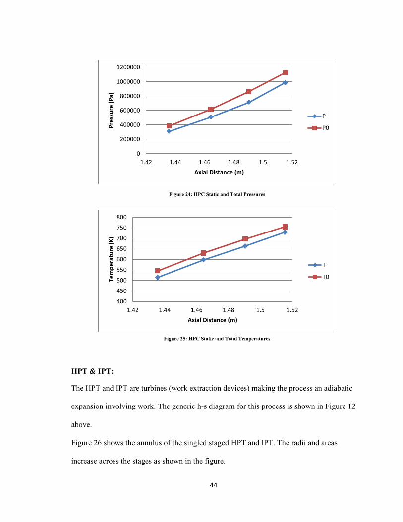
HPT & IPT:

The HPT and IPT are turbines (work extraction devices) making the process an adiabatic

expansion involving work. The generic h-s diagram for this process is shown in Figure 12

above.

Figure 26 shows the annulus of the singled staged HPT and IPT. The radii and areas

increase across the stages as shown in the figure.

0

200000

400000

600000

800000

1000000

1200000

1.42 1.44 1.46 1.48 1.5 1.52

Pres

sure

(Pa)

Axial Distance (m)

P

P0

400

450

500

550

600

650

700

750

800

1.42 1.44 1.46 1.48 1.5 1.52

Tem

pera

ture

(K)

Axial Distance (m)

T

T0

Figure 24: HPC Static and Total Pressures

Figure 25: HPC Static and Total Temperatures

45

The HPT and IPT pressures and temperatures are graphed below in Figures 27 and 28

respectively. Since turbines are expansion devices, the pressures and temperatures across

it tend to drop as can be seen from the figures.

0.4

0.41

0.42

0.43

0.44

0.45

0.46

0.47

0.48

0.49

0.5

0.51

0.52

0.53

0.54

0.55

0.56

1.8 1.81 1.82 1.83 1.84 1.85 1.86 1.87 1.88 1.89 1.9

Heig

ht (m

)

Axial Distance (m)

Figure 26: Annulus of Single Staged HPT and IPT

46

Figure 14: HPT and IPT static and total pressures

1100

1200

1300

1400

1500

1600

1700

1800

1.78 1.83 1.88 1.93 1.98

Tem

pera

ture

(K)

Axial Distance (m)

T

T0

0

200000

400000

600000

800000

1000000

1200000

1.78 1.8 1.82 1.84 1.86 1.88 1.9

Pres

sure

(Pa)

Axial Distance (m)

P

P0

Figure 27: HPT/IPT Static and Total Pressures

Figure 28: HPT and IPT Static and Total Temperatures

47

LPT

The LPT, like the HPT and IPT is device work device making the process an adiabatic

expansion one involving work. The generic h-s diagram for this process is given in

Figure 12 above. The six staged LPT is responsible for powering the primary and

secondary fans. The geometry is similar to that of the GE90 where the hub and tip climb

initially and then level out. Figure 29 below shows the annulus of the LPT.

Figures 30 and 31 below show the LPT pressures and temperatures trend. As expected,

due to the expansion process, the pressures and temperatures drop across the turbine.

0.6

0.65

0.7

0.75

0.8

0.85

0.9

0.95

2.2 2.25 2.3 2.35 2.4 2.45 2.5 2.55 2.6 2.65 2.7 2.75 2.8 2.85 2.9 2.95 3

Heig

ht (m

)

Axial Distance (m)

Figure 29: Annulus of Six Staged LPT

48

Overall Engine

The h-s diagram for the HDBPE core is provided below in Figure 32.

0

50000

100000

150000

200000

250000

300000

350000

400000

2.15 2.35 2.55 2.75 2.95 3.15

Pres

sure

(Pa)

Axial Distance (m)

P

P0

600

700

800

900

1000

1100

1200

1300

1400

2.15 2.35 2.55 2.75 2.95 3.15

Tem

pera

ture

(K)

Axial Distance (m)

T

T0

Figure 30: LPT Static and Total Pressures

Figure 31: LPT Static and Total Temperatures

49

Section A of the graph above represents the compression process in the engine, i.e.

compression across the fans, IPC, and HPC. Compression increases the total enthalpy of

the system, but does so only over a smaller range of entropy. Section B on the graph

represents the combustion process in the engine. During combustion there is an increase

in total enthalpy but over a larger entropy range. Total enthalpy is the amount of energy

available to do useful work and since combustion increases the energy of the gas

available, the increase in total enthalpy is significant. Section C of the graph represents

the expansion process that the gas undergoes when going through the turbine section of

the engine. The HPT, IPT, and LPT are work extracting devices that result in a decrease

in the total enthalpy of the system.

Figure 32: Core h-s Diagram

50

Tables 8, 9, and 10 below highlight the major design choices and results associated with

the calculations that were done manually in Excel using the Brayton Cycle analysis.

Table 8: Important Cruise Design Choices and Results

Cruise T.I.T (K) 1,700.00

Fuel mass flow rate (Kg/s) 1.50 Overall pressure ratio 35.65

Fan Diameter (in.) 120.63 Thrust (lbf) 18464.91

SFC (lbm/hr.lbf) 0.6457

Table 9: Mass Flow Rates at Cruise

Cruise Incoming net mass flow rate (Kg/s) 515.12

Core mass flow (Kg/s) 51.52 Outer bypass mass flow rate (Kg/s) 367.95 Inner bypass mass flow rate (Kg/s) 95.66

Table 10: Compressor RPM's at Cruise

Cruise Primary fan RPM 2500.00

Secondary fan RPM 4800.00 Intermediate pressure spool RPM 5698.00

High pressure spool RPM 9637.00

The T.I.T chosen was 1,700 K. The thrust generated was 18,465 lbf leading to an SFC of

0.6457 (lbm/hr.lbf). The incoming mass flow rate was 515.12 Kg/S establishing a fan tip

diameter of 120.63 in. The inner and outer bypass ratios were 2.5 and 1.857 respectively,

leading to an overall bypass ratio of 9. The mass flow rates through the three distinct

routes are given above in Table 9. The overall pressure ratio was 35.65 and this was a

product of the compressor total pressure ratios. The compressor rpms are provided in

Table 10 above.

51

Figure 33 below is the meridional view of the HDBPE. The engine length from the fan to

the LPT exit is 2.76 meters (108.66 inches) while the fan tip diameter is 3.06 meters

(120.63 inches).

52

Figure 33: HDBPE Overall Engine Meridional View

53

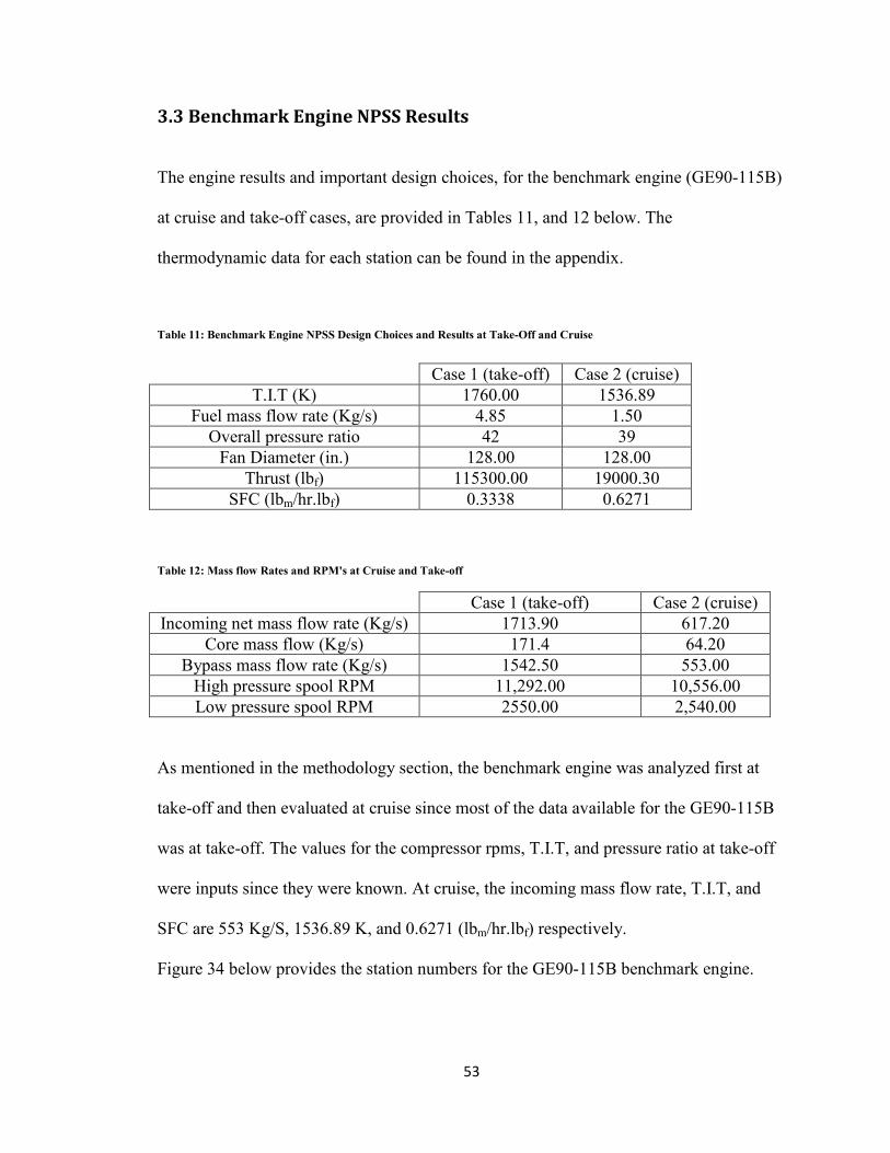
3.3 Benchmark Engine NPSS Results

The engine results and important design choices, for the benchmark engine (GE90-115B)

at cruise and take-off cases, are provided in Tables 11, and 12 below. The

thermodynamic data for each station can be found in the appendix.

Table 11: Benchmark Engine NPSS Design Choices and Results at Take-Off and Cruise

Table 12: Mass flow Rates and RPM's at Cruise and Take-off

Case 1 (take-off) Case 2 (cruise) Incoming net mass flow rate (Kg/s) 1713.90 617.20

Core mass flow (Kg/s) 171.4 64.20 Bypass mass flow rate (Kg/s) 1542.50 553.00

High pressure spool RPM 11,292.00 10,556.00 Low pressure spool RPM 2550.00 2,540.00

As mentioned in the methodology section, the benchmark engine was analyzed first at

take-off and then evaluated at cruise since most of the data available for the GE90-115B

was at take-off. The values for the compressor rpms, T.I.T, and pressure ratio at take-off

were inputs since they were known. At cruise, the incoming mass flow rate, T.I.T, and

SFC are 553 Kg/S, 1536.89 K, and 0.6271 (lbm/hr.lbf) respectively.

Figure 34 below provides the station numbers for the GE90-115B benchmark engine.

Case 1 (take-off) Case 2 (cruise) T.I.T (K) 1760.00 1536.89

Fuel mass flow rate (Kg/s) 4.85 1.50 Overall pressure ratio 42 39

Fan Diameter (in.) 128.00 128.00 Thrust (lbf) 115300.00 19000.30

SFC (lbm/hr.lbf) 0.3338 0.6271

54

The pressure and temperature diagrams for the benchmark engine are provided below.

For the core h-s diagram and explanation refer to Figure 32.

0

200

400

600

800

1000

1200

1400

1600

1800

1 2 3 4 5 6 7 8 9 10 11 12 13 14

Tem

[era

ture

(K)

Flow Station

T0(K)

T(K)

Figure 35: Benchmark Engine Static and Total Temperatures

Figure 34: Benchmark Engine Station Numbering

55

0

0.2

0.4

0.6

0.8

1

1.2

1.4

1.6

1 2 3 4 5 6 7 8 9 10 11 12 13 14

Pres

suur

e (M

Pa)

Flow Station

P0(Pa)

P(Pa)

Figure 36: Benchmark Engine Static and Total Pressures

56

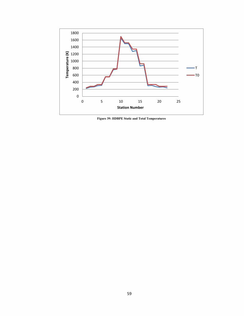
3.4 HDBPE NPSS Results

NPSS is an industry standard software that can be used to model any gas turbine engine

configuration that other currently available programs are incapable of. Most engine

modeling programs have built-in standard engine architecture while NPSS can be

programmed to accommodate any kind of engine configuration and is a great tool to

model innovative engine architecture. NPSS has several thermodynamic packages readily

available for the user. Some of the packages include GasTbl developed by Pratt &

Whitney, allFuel developed by General Electric, Janaf developed by Honeywell, and

CEA which is NASA’s chemical equilibrium package. The student learning edition was

used for this thesis and as a result the full functional capabilities of NPSS were not

available. However, the cycle analysis performed in NPSS was done at an extremely high

fidelity and was sufficient in order to analyze the HDBPE concept.

NPSS was used to analyze the HDBPE at cruise and also evaluate it at take-off. Major

focus was on the cruise performance of the engine, however take-off was also checked in

order to ensure that the engine was capable of taking off without violating the constraint

imposed on the T.I.T. Tables 13, 14, and 15 below show the HDBPE performance at

cruise (Case 1) and take-off (Case 2). The thermodynamic data for each station can be

found in the appendix

57

Table 13: Important HDBPE NPSS Results at Cruise and Take-off

Case 1 (Cruise) Case 2 (Take-off) T.I.T (K) 1,700.00 1,994.19

Fuel mass flow rate (Kg/s) 1.4765 5.4234 Overall pressure ratio 35.65 37.203

Fan Diameter (in.) 120.63 120.63 Thrust (lbf) 19,000.50 115,300.10

SFC (lbm/hr.lbf) 0.6167 0.3733

Table 14: Mass Flow Rates at Cruise and Take-Off

Case 1 (Cruise) Case 2 (Take-off) Incoming net mass flow rate (Kg/s) 508.6 1,464.10

Core mass flow (Kg/s) 50.50 149.50 Outer bypass mass flow rate (Kg/s) 363.3 1037.80 Inner bypass mass flow rate (Kg/s) 94.8 276.70

Table 15: Compressor RPM's at Cruise and Take-Off

Case 1 (Cruise) Case 2 (Take-off) Primary fan RPM 2,500.00 2,742.00

Secondary fan RPM 4,800.00 5,264.00 Intermediate pressure spool RPM 5,698.00 6,219.00

High pressure spool RPM 9,637.00 10,435.00

From Table 13 it can be seen that the T.I.T is less than 2,100K which is the current

industry standard maximum value. The intake mass flow rate is 508.6 Kg/S while the fuel

mass flow rate is 1.4765 Kg/S. The thrust delivered at cruise is 19,000 lbs, the same as

that of the benchmark engine, thus making the SFC 0.6167 (lbm/hr.lbf). The engine

station numbers are provided below in Figure 37. Following this are the thermodynamic

graphs pertaining to temperatures and pressures. Refer to Figure 32 for the core h-s

diagram and explanation.

58

Figures 38 and 39 below show the pressures and temperatures trend for the HDBPE that

was analyzed using NPSS.

0

200000

400000

600000

800000

1000000

1200000

1400000

0 5 10 15 20 25

Pres

sure

(Pa)

Station Number

P

P0

Figure 37: HDBPE Station Numbering

Figure 38: HDBPE Static and Total Pressures

59

0

200

400

600

800

1000

1200

1400

1600

1800

0 5 10 15 20 25

Tem

pera

ture

(K)

Station Number

T

T0

Figure 39: HDBPE Static and Total Temperatures

60

3.5 HDBPE – Benchmark Engine NPSS Comparison.

Tables 16, 17, and 18 below illustrate the comparison, at cruise, between the HDBPE and

benchmark engine analyzed in NPSS. The red highlights are the most important

comparisons.

Table 16: HDBPE and Benchmark Engine NPSS Cruise Comparison

HDBPE Benchmark T.I.T (K) 1,700.00 1,536.89

Fuel mass flow rate (Kg/s) 1.4765 1.50 Overall pressure ratio 35.65 39.00 Overall bypass ratio 9.063 9.00 Fan diameter (in.) 120.63 128.00

Thrust (lbf) 19,000.00 19,000.30 SFC (lbm/hr.lbf) 0.6114 0.6271

Engine length from fan to LPT (m) 2.76 4.66

Table 17: HDBPE and Benchmark Engine Mass Flow Rates

HDBPE Benchmark Incoming net mass flow rate (Kg/s) 508.60 617.20

Core mass flow (Kg/s) 50.70 64.20 Outer bypass mass flow rate (Kg/s) 364.70 553.00 Inner bypass mass flow rate (Kg/s) 95.10 N/A

Table 18: HDBPE and Benchmark Engine Compressor RPM's

HDBPE Benchmark Primary fan RPM 2,500.00 2,540.00

Secondary fan RPM 4,800.00 N/A Intermediate pressure spool RPM 5,698.00 N/A

High pressure spool RPM 9,637.00 10,556.00

It can be seen from the tables above that the HDBPE has some clear advantages when

compared to the benchmark engine, GE90-115B. The main focus is on the cruise analysis

so values pertaining to cruise condition shall be discussed here. Both the engines belong

61

to the same thrust class, i.e. both engines are capable of producing 19,000 lbs of thrust at

cruise. However, the HDBPE is able to do so by being much smaller in size. The HDBPE

is 2.76 meters long (measured from fan inlet to LPT exit) while having a fan tip diameter

of 120.63 in. The benchmark engine is 4.66 meters long (also measured from fan inlet to

LPT exit) with a fan tip diameter of 128.00 in. Another significant performance

parameter to be considered is the SFC which determines how fuel efficient the engine is.

The SFC is defined as follows:

𝑆𝐹𝐶 = �̇�𝑓

𝑇 (22)

The thrust capability of both engines, as mentioned before, is the same thus making SFC

directly proportional to the fuel mass flow rate. The fuel consumed by the HDBPE is

lower than that of the benchmark engine, making the HDBPE more fuel efficient (lower

SFC); the reduction in SFC is 2.5%. The HDBPE has a higher T.I.T than that of the

benchmark engine leading to higher thermal stresses in the engine and a lower life span.

However, the difference in T.I.T is only 163K and by taking into account the amount of

fuel saved over a time frame by the HDBPE, this disadvantage is minor. The following

illustrates the amount of fuel that can be saved when using the HDBPE:

From Table 16 above, the fuel mass flow rates for the HDBPE and the benchmark engine

are 1.4765Kg/S and 1.50 Kg/S respectively, and the difference between the two mass

flow rates is 0.0235 Kg/S. Assuming that the cruise time (tcr) is 10 hours, then the

difference in mass flows (Δmfcr) is the product between the cruise time and mass flow

rate difference. Thus:

∆𝑚𝑓𝑐𝑟 = 10 × 3,600 × 0.0235 (23)

62

∆𝑚𝑓𝑐𝑟 = 846 𝐾𝑔 = 1,865.112 𝑙𝑏𝑠 (24)

For a twin engine aircraft:

∆𝑚𝑓𝑐𝑟 = 2 × 3,174.62 𝑙𝑏𝑠 = 3,730.22 𝑙𝑏𝑠 (25)

A gallon of Jet-A fuel is 6.67 lbs, so:

𝐹𝑢𝑒𝑙 𝑠𝑎𝑣𝑒𝑑 = 3,730.22

6.67= 559.25 𝑔𝑎𝑙𝑙𝑜𝑛𝑠 (26)

Currently, a gallon of Jet-A fuel costs on average $5.62. Hence, the total cost saved is:

𝐴𝑚𝑜𝑢𝑛𝑡 𝑠𝑎𝑣𝑒𝑑 = 5.62 × 559.25 = $3,143 (27)

The total cost saved seems to be a small amount, but this is only for a 10 hour long

cruise. The amount saved over a period of time is significant and needs to be considered.

Figure 40 below shows the length comparison between the HDBPE and the benchmark

engine. The HDBPE was placed on top of the scaled benchmark engine to illustrate the

comparison.

63

Figure 40: HDBPE and Benchmark Engine Length Comparison

64

3.6 HDBPE Basic Sensitivity Analysis

This section discusses the sensitivity of the HDBPE to some important variables such as

the outer and inner bypass ratios, and T.I.T. All variables were kept constant at their base

design value and the desired parameter was then varied in order to study its consequent

effect. It is important to note that when changing a parameter of interest, the thrust and

SFC change. It is desired to maintain the thrust level the same as that of the benchmark

engine. For example, it will be seen that an increase in bypass ratio, up to a certain point,

decreases the SFC. This means that the engine becomes more fuel efficient with

increased Bypass ratio. However, an increase in bypass ratio decreases the thrust, and to

maintain the required thrust level the T.I.T has to be increased or the incoming mass flow

needs to be increased (i.e. the fan diameter increases). It will be illustrated that an

increase in T.I.T, after a certain point, increases the SFC thus making the engine less fuel

efficient. To reduce this negative effect, the incoming mass flow can be increased. It can

be seen that this is an iterative process and several iterations need to be done.

Some sensitivity tests were available for the GE90-85B engine, which is rated at 85,000

lbf. Figures 41 and 42 below illustrate the effect that bypass ratio and T.I.T have on

engine thrust and SFC, respectively, at cruise for the GE90-85B engine, a smaller

derivative. The trends are same as that for the GE90-115B engine but the values differ.

65

Figure 41: Effect of Bypass Ratio on Engine Thrust and SFC for GE90-85B. [9]

Figure 42: Effect of T.I.T on Engine Thrust and SFC for GE90-85B. [9]

66

The following discussion pertains to the effect of outer and inner bypass ratios, and T.I.T

on engine thrust and cruise for the HDBPE. The trends are same as those for the

published GE90-85B trends.

Effect of outer bypass ratio:

Figures 43 and 44 illustrate the effect that the outer bypass ratio has on the thrust and

SFC of the engine respectively.

05000

10000150002000025000300003500040000

0 1 2 3 4 5 6

Thru

st (l

b f)

Outer Bypass Ratio

0

0.2

0.4

0.6

0.8

1

1.2

1.4

0 1 2 3 4 5 6

SFC

(lbm

/hr.l

b f)

Outer Bypass Ratio

Figure 43: Effect of Outer Bypass Ratio on Engine Thrust for HDBPE

Figure 44: Effect of Outer Bypass Ratio on Engine SFC for HDBPE

67

Figure 43 demonstrates the fact that as the outer bypass ratio increases, the engine thrust

decreases in an almost linear manner. However, the effect of the outer bypass ratio on the

SFC is more complex. As the bypass ratio increases the SFC tends to drop and at a

bypass value of 3.2 the SFC is at its lowest. After this, the SFC increases exponentially

with respect to the outer bypass ratio.

Effect of inner bypass ratio:

Figures 45 and 46 illustrate the effect that the inner bypass ratio has on the thrust and

SFC of the engine respectively.

The effect of the inner bypass ratio on the engine thrust follows the same trend as that of

the effect of the outer bypass ratio on engine thrust; the engine thrust decreases in an

almost linear manner.

0

5000

10000

15000

20000

25000

30000

35000

40000

0 0.5 1 1.5 2 2.5 3 3.5 4

Thru

st (l

b f)

Inner Bypass Ratio

Figure 45: Effect of Inner Bypass Ration on Engine Thrust

68

The effect of inner bypass ratio on engine SFC also follows the same general trend as that

of the effect of the outer bypass ratio on engine SFC; the SFC drops and then increases

exponentially with respect to the inner bypass ratio.

Since the HDBPE is focused more on improving the engine SFC, it may be appropriate to

select the combination of the two bypass ratios such that the SFC is at its lowest.

However, the amount of thrust that the engine is capable of producing must also be taken

into account. At bypass ratios favoring SFC, the engine thrust drops by a large amount.

Also, it must be noted that the above graphs were generated by keeping the other

parameters at their base values while evaluating the parameter of interest. Thus, in order

to get the optimal combination of bypass ratios, several iterations were done to determine

the values. To achieve the desired results, the outer bypass ratio was determined to be

3.15 and the inner bypass ratio was determined to be 1.857, making the overall bypass

ratio 10.857.

0

0.2

0.4

0.6

0.8

1

1.2

1.4

0 0.5 1 1.5 2 2.5 3 3.5 4

SFC

(lbm

/hr.l

b f)

Inner Bypass Ratio

Figure 46: Effect of Inner Bypass ratio on Engine SFC

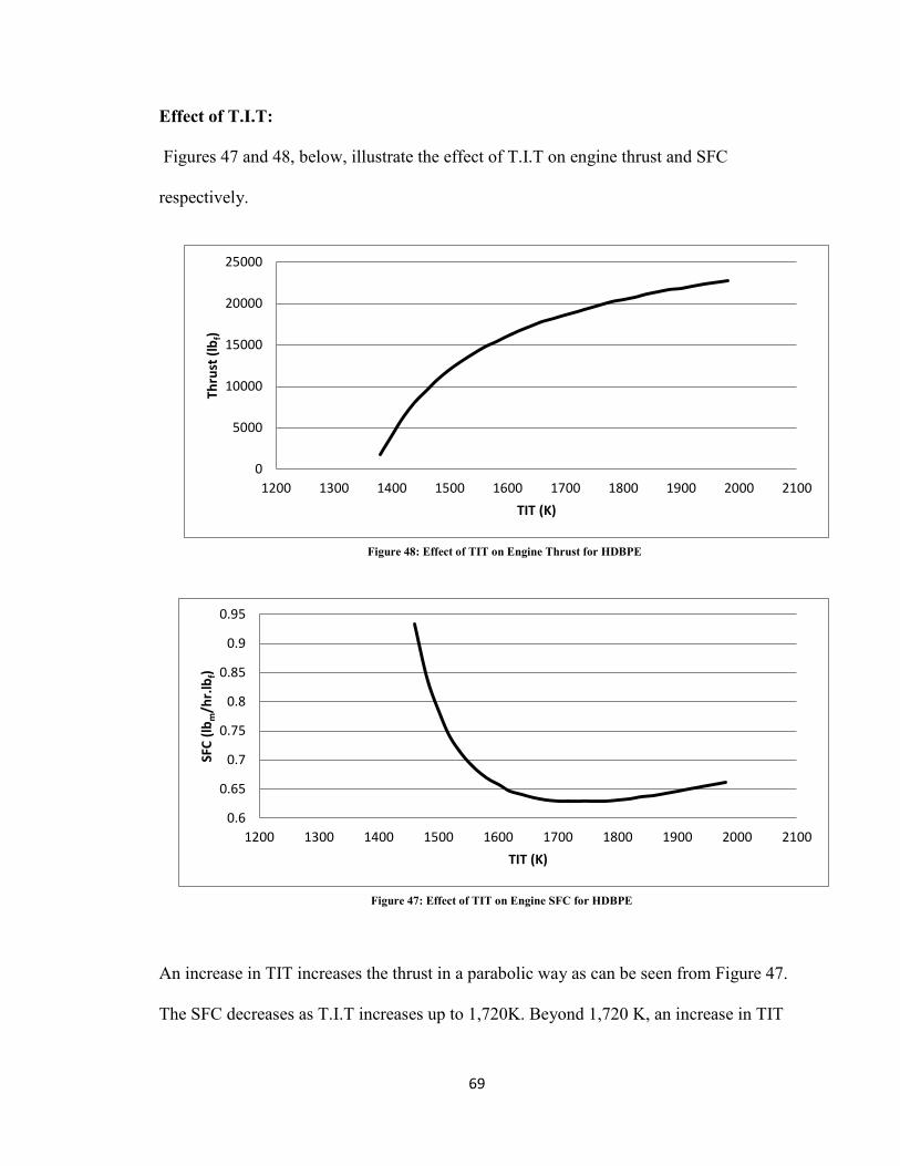
69

Effect of T.I.T:

Figures 47 and 48, below, illustrate the effect of T.I.T on engine thrust and SFC

respectively.

An increase in TIT increases the thrust in a parabolic way as can be seen from Figure 47.

The SFC decreases as T.I.T increases up to 1,720K. Beyond 1,720 K, an increase in TIT

0.6

0.65

0.7

0.75

0.8

0.85

0.9

0.95

1200 1300 1400 1500 1600 1700 1800 1900 2000 2100

SFC

(lbm

/hr.l

b f)

TIT (K)

0

5000

10000

15000

20000

25000

1200 1300 1400 1500 1600 1700 1800 1900 2000 2100

Thru

st (l

b f)

TIT (K)

Figure 47: Effect of TIT on Engine SFC for HDBPE

Figure 48: Effect of TIT on Engine Thrust for HDBPE

70

results in an increase in SFC. Therefore, in order to be more fuel efficient than the

benchmark engine, the T.I.T was selected to be 1,720 K.

In order to verify the new results obtained, NPSS was run again with the new bypass

ratios and T.I.T. The new overall bypass ratio is an increase compared to the base overall

bypass ratio of 9.063. The increase in bypass ratio dropped the thrust and in order to

maintain the HDBPE as the same thrust class as the benchmark engine, the incoming

mass flow was increased. This was proved in NPSS. The following tables provide the

important results obtained from NPSS. The comparison discussion pertains to the base

HDBPE and the optimized HDBPE only.

Table 19: NPSS Important Design Choices and Results

Table 20: Mass Flow Rates of the New Engine

Cruise T.I.T (K) 1,720.00

Inner bypass ratio 1.857 Outer bypass ratio 3.150

Overall bypass ratio 10.857 Fan Diameter (in.) 124.31

Thrust (lbf) 19,000.00 SFC (lbm/hr.lbf) 0.5975

Cruise Incoming net mass flow rate (Kg/s) 564.80

Core mass flow (Kg/s) 47.60 Outer bypass mass flow rate (Kg/s) 428.7 Inner bypass mass flow rate (Kg/s) 88.50

Fuel mass flow rate (Kg/s) 1.43

71

Table 21: RPMs of the New Engine

Cruise Primary fan RPM 2,500.00

Secondary fan RPM 4,800.00 Intermediate pressure spool RPM 5,719.00

High pressure spool RPM 9,637.00

From the above Tables, it can be seen that the overall bypass ratio and T.I.T have

increased compared to their base values of 9.0 and 1,700 K respectively. The SFC

dropped comparatively by 3.1 %. The mass flow rate increased leading to a 2.96%

increase in fan diameter. The new fan tip diameter is 124.31 inches, but it is still smaller

than that of the benchmark engine. The RPMs, were almost the same as their base values.

After running the fuel saved calculation it was determined that the amount of fuel saved

was 1,666 gallons when compared to the benchmark engine. Also, the total cost saved

was $ 9,362 and this is a 197.9% increase compared to the base HDBPE. Table 22 below

illustrates the comparison.

Table 22: Base HDBPE and Optimized HDBPE Comparison

Base HDBPE Optimized HDBPE % Difference Incoming mass flow (Kg/S) 508.6 564.80 11.05

Fan diameter (in) 120.63 124.31 3.05 Total fuel cost saved ($) 3,143 9,362 197.90

SFC (lbm/hr.lbf) 0.6167 0.5975 3.10 T.I.T (K) 1,700 1,720 1.17

72

4 CONCLUSIONS AND RECOMMENDATIONS

The HDBPE was first analyzed manually using conventional thermodynamics, free

vortex radial equilibrium, and the Euler turbomachinery equation. Microsoft Excel was

used for this analysis. Next, the HDBPE was set up in NPSS and the analysis was

performed. The results obtained from NPSS were then validated with the results from

Excel and were found to be within 4% error. The benchmark engine, GE90-115B, was

reverse-engineered using Excel and later analyzed in NPSS using the available

information. Most information was available at take-off so the engine was first analyzed

at take-off in NPSS and then at cruise.

The HDBPE and the benchmark engine belong to the same thrust class, but it can be

concluded that the HDBPE is much shorter in length, has a smaller fan tip diameter, and

is more fuel efficient and is thus superior to its competitor. The T.I.T of the HDBPE is

higher than that of the benchmark engine and this may lead to larger thermal stresses in

the combustion chamber and hence a reduced lifespan. However, when considering the

fuel saving capacity of the engine and the smaller size, this disadvantage is outweighed.

A basic sensitivity analysis was run on the base HDBPE and it was concluded that the

engine could be more efficient if it was made larger in diameter with the outer and inner

bypass ratios, and T.I.T being 3.15, 1.857, and 1,720 K respectively.

In order to increase engine performance, CFD analysis recommended since this is an

innovative concept in the commercial transportation industry. Bleed ports could have

been modeled in order to get a more accurate result for the HDBPE and benchmark

73

engines. Also, other kinds of engine configurations could be considered to improve

engine performance. The following are the possible configurations:

• Primary fan counter-rotating with the secondary fan

• Mixing of the inner bypass stream and the core

• Mounting the secondary fan to the same shaft as that of the IPC

74

5 REFERENCES

1. “Background, Development, and, Theory,” 3 August 2011 <http://www.aircav.com/histturb.html

2. “Gas Turbine History,” 30 September 2011 <http://www.turbomachine.com/history/>

3. “Aviation History,” 30 September 2011 <http://www.wingsoverkansas.com/history/article.asp?id=1031

4. Simmons, R.J., 2009, “Design and Control of a Variable Geometry Turbofan with an Independently Modulated Third Stream.” MS Thesis, Ohio State University, Ohio, OH

5. “The Advent of a Better Jet Engine?” 30 September 2011 <http://www.defenseindustrydaily.com/the-advent-of-a-better-jet-engine-03623/>

6. Attia, M.S., 2010, “Embry-Riddle Aeronautical University AE 440 (Detailed Air Breathing Propulsion Design) Class Notes,” Daytona Beach, FL.

7. Schobeiri, M., 2005, Turbomachinery Flow Physics and Dynamic Performance, Springer-Verlag Berlin Heidelberg.

8. “GE90 Engine Airflow,” 30 September 2011 <http://www.google.com/imgres?imgurl=http://ctr-sgi1.stanford.edu/CITS/ge90r.jpeg&imgrefurl=http://ctr-sgi1.stanford.edu/CITS/ge90.html&usg=__yhs-scWqxXRIcX6WjjcrsUSa8IE=&h=1197&w=1523&sz=804&hl=en&start=11&zoom=1&tbnid=ECqixALhgdYw2M:&tbnh=118&tbnw=150&ei=IvCJToyUIcjKgQeF_aX6Cg&prev=/search%3Fq%3DGE90%2Bengine%26hl%3Den%26safe%3Doff%26sa%3DX%26biw%3D1280%26bih%3D937%26tbm%3Disch%26prmd%3Divns&itbs=1>

9. “The GE-90 an Introduction,” 1-18., 30 September 2011 <http://www.stanford.edu/~cantwell/AA283_Course_Material/GE90_Engine_Data.pdf>

10. Boyce, M.P., 2006, Gas Turbine Engineering Handbook, 3rd Edition, Elsevier 11. Cumpsty,N.A., 1989, Compressor Aerodynamics, Addison Wesley Longman

Limited 12. El-Sayed, A., 2008, Aircraft Propulsion and Gas Turbines Engines, CRC Taylor

& Francis Group. 13. Falck, N., February 2008, “Axial Flow Compressor Mean Line Design,” MS

Thesis, Lund University, Sweden 14. Hemerly, C., Attia, M.S., 2006, “Modular Multi-Stage Axial Compressor

Design: A Lean Approach,” Lean Aerospace Initiative Plenary Conference, April 19-20, Texas, TX.

15. Hill, P., & Peterson, C., 1992, Mechanics and Thermodynamics of Propulsion, 2nd Edition, Addison-Wesley Publishing Company, Inc.

16. Lieblein, S., Schwenk, F.’ & Broderick, R.L., June 1953., “Diffusion Factor for Estimating Losses and Limiting Blade Loadings in Axial-Flow-Compressor Blade Elements, Cleveland, OH

75

17. Mattingly, J., Heiser, W., & Pratt, D., 2002, Aircraft Engine Design, 2nd Edition, American Institute of Aeronautics and Astronautics, Inc.

76

6 APPENDIX

The following is the data sheet for the station thermodynamic results produced by NPSS

for the HDBPE.

All units are in SI unless indicated otherwise, Model was run at 12:00:08 on 09/22/11 Ambient Prim. Fan Inlet Prim. Fan Exit mdot(kg/sec) 508.6 508.6 508.6 Gamma 1.401229 1.401223 1.401205 T0(K) 247.3 247.3 287.3 T(K) 216.7 222.2 260.7 P0(Pa) 32778.3 32614.4 52183.1 P(Pa) 20645.9 22453.0 37139.0 Total Mach 0.840 0.750 0.714 A(m2) 6.1777 6.4437 4.4319 A(in2) 9575.399 9987.711 6869.534 h(J/kg) 216632.777 222235.404 260772.265 h0(J/kg) 247375.602 247375.602 287498.772 rho(kg/m3) 0.3320 0.3520 0.4963 Speed of Sound(m/sec) 295.19 298.98 323.81 Total Velcocity (m/sec) 247.963 224.233 231.199 R (J/(kg*K)) 287.043 287.043 287.043 s(J/kg) -304.12699 -303.32762 -294.73056 All units are in SI unless indicated otherwise, Model was run at 12:00:08 on 09/22/11 Sec. Fan Inlet Sec. Fan Exit IPC Inlet mdot(kg/sec) 145.3 145.3 50.5 Gamma 1.401064 1.400023 1.399589 T0(K) 287.3 332.4 332.4 T(K) 267.9 302.3 314.9 P0(Pa) 52183.1 82449.2 82449.2 P(Pa) 40872.5 59125.8 68195.1 Total Mach 0.601 0.706 0.528 A(m2) 1.3859 0.8666 0.3567 A(in2) 2148.122 1343.222 552.874 h(J/kg) 268038.006 302522.258 315165.288 h0(J/kg) 287498.772 332798.755 332798.755 rho(kg/m3) 0.5314 0.6814 0.7545 Speed of Sound(m/sec) 328.26 348.55 355.67 Total Velcocity (m/sec) 197.285 246.075 187.795 R (J/(kg*K)) 287.043 287.043 287.043 s(J/kg) -294.73056 -286.34227 -286.34227 All units are in SI unless indicated otherwise, Model was run at 12:00:08 on 09/22/11 IPC Exit HPC Inlet HPC Exit mdot(kg/sec) 50.5 50.5 50.5 Gamma 1.382222 1.382576 1.359271 T0(K) 549.2 549.2 763.9 T(K) 542.0 538.8 746.2 P0(Pa) 399219.1 398875.4 1161525.2 P(Pa) 380712.8 372364.3 1062657.0 Total Mach 0.263 0.317 0.364 A(m2) 0.1693 0.1432 0.0519 A(in2) 262.487 221.972 80.392 h(J/kg) 546473.298 543166.314 763174.992 h0(J/kg) 553910.870 553910.870 782462.338 rho(kg/m3) 2.4470 2.4075 4.9614 Speed of Sound(m/sec) 463.74 462.43 539.57 Total Velcocity (m/sec) 121.964 146.592 196.404 R (J/(kg*K)) 287.043 287.043 287.043 s(J/kg) -253.67415 -253.53679 -229.12971

77

All units are in SI unless indicated otherwise, Model was run at 12:00:08 on 09/22/11 CC Inlet HPT Inlet HPT Exit mdot(kg/sec) 50.5 52.0 52.0 Gamma 1.357591 1.284527 1.289851 T0(K) 763.9 1700.0 1527.9 T(K) 761.8 1662.2 1496.1 P0(Pa) 1156244.9 1144682.5 656397.4 P(Pa) 1144063.1 1034245.1 597750.7 Total Mach 0.125 0.400 0.383 A(m2) 0.1418 0.0766 0.1311 A(in2) 219.841 118.762 203.181 h(J/kg) 780143.143 1907720.801 1694057.840 h0(J/kg) 782462.338 1956739.152 1734674.945 rho(kg/m3) 5.2320 2.1682 1.3923 Speed of Sound(m/sec) 544.85 782.77 744.17 Total Velcocity (m/sec) 68.106 313.108 285.016 R (J/(kg*K)) 287.043 286.970 286.970 s(J/kg) -228.40311 332.72726 344.88885 All units are in SI unless indicated otherwise, Model was run at 12:00:08 on 09/22/11 IPT Inlet IPT Exit LPT Inlet mdot(kg/sec) 52.0 52.0 52.0 Gamma 1.289851 1.298416 1.297275 T0(K) 1527.9 1358.7 1358.7 T(K) 1496.1 1289.5 1312.9 P0(Pa) 656397.4 359417.9 358291.5 P(Pa) 597750.7 285933.5 308346.7 Total Mach 0.383 0.601 0.485 A(m2) 0.1311 0.1616 0.1874 A(in2) 203.181 250.469 290.545 h(J/kg) 1694057.840 1433063.746 1462352.497 h0(J/kg) 1734674.945 1519839.053 1519839.053 rho(kg/m3) 1.3923 0.7727 0.8184 Speed of Sound(m/sec) 744.17 693.17 699.13 Total Velcocity (m/sec) 285.016 416.593 339.077 R (J/(kg*K)) 286.970 286.970 286.970 s(J/kg) 344.88885 358.14849 358.64892 All units are in SI unless indicated otherwise, Model was run at 12:00:08 on 09/22/11 LPT Exit LPT Stator Exit Core Nozzle Exit mdot(kg/sec) 52.0 52.0 52.0 Gamma 1.326769 1.324796 1.333747 T0(K) 934.4 934.4 934.4 T(K) 874.8 896.6 802.4 P0(Pa) 53992.0 53512.1 53512.1 P(Pa) 41240.9 45168.9 28874.0 Total Mach 0.648 0.511 1.000 A(m2) 0.8466 0.9931 0.7485 A(in2) 1312.307 1539.362 1160.242 h(J/kg) 931087.164 956514.202 847452.848 h0(J/kg) 1001015.866 1001015.866 1001015.866 rho(kg/m3) 0.1643 0.1756 0.1254 Speed of Sound(m/sec) 577.12 583.82 554.19 Total Velcocity (m/sec) 373.973 298.334 554.190 R (J/(kg*K)) 286.970 286.970 286.970 s(J/kg) 406.43289 407.85622 407.85622 All units are in SI unless indicated otherwise, Model was run at 12:00:08 on 09/22/11 IBP Stator Inlet IBP Stator Exit IBP Nozzle Exit mdot(kg/sec) 94.8 94.8 94.8 Gamma 1.400023 1.399606 1.400842 T0(K) 332.4 332.4 332.4 T(K) 302.3 314.4 277.0 P0(Pa) 82449.2 81493.7 81493.7 P(Pa) 59125.8 67025.8 43044.2

78

Total Mach 0.706 0.536 1.000 A(m2) 0.5652 0.6698 0.5245 A(in2) 876.014 1038.139 812.938 h(J/kg) 302522.258 314655.919 277110.198 h0(J/kg) 332798.755 332798.755 332798.755 rho(kg/m3) 0.6814 0.7427 0.5414 Speed of Sound(m/sec) 348.55 355.39 333.73 Total Velcocity (m/sec) 246.075 190.488 333.731 R (J/(kg*K)) 287.043 287.043 287.043 s(J/kg) -286.34227 -284.48340 -284.48340 All units are in SI unless indicated otherwise, Model was run at 12:00:08 on 09/22/11 OBP Stator Inlet OBP Nozzle Inlet OBP Nozzle Exit mdot(kg/sec) 363.3 363.3 363.3 Gamma 1.401205 1.401034 1.401330 T0(K) 287.3 287.3 287.3 T(K) 260.7 269.2 239.3 P0(Pa) 52183.1 51661.2 51661.2 P(Pa) 37139.0 41157.8 27277.4 Total Mach 0.714 0.579 1.000 A(m2) 3.1657 3.5802 2.9486 A(in2) 4906.810 5549.266 4570.263 h(J/kg) 260772.265 269348.927 239364.278 h0(J/kg) 287498.772 287498.772 287498.772 rho(kg/m3) 0.4963 0.5325 0.3971 Speed of Sound(m/sec) 323.81 329.06 310.27 Total Velcocity (m/sec) 231.199 190.525 310.272 R (J/(kg*K)) 287.043 287.043 287.043 s(J/kg) -294.73056 -293.12785 -293.12785

The following is the HDBPE major performance parameters obtained from NPSS for

cruise and take-off.

All units are in SI unless indicated otherwise, Model was run at 12:00:08 on 09/22/11 Case 1 Case 2 Alt(ft) 38000 0 Mach 0.84 0.00 mdoti 508.6 1464.1 mdotc 50.5 149.5 mdotOBP 363.3 1037.8 mdotIBP 94.8 276.7 T.I.T 1700.00 1994.19 RPM_LP 2500 2742 RPM_IP 5698 6219 RPM_HP 9637 10435 RPM_Sec_Fan 4800 5264 mdotf 1.4765 5.4234 Overall_Pressure_Ratio 35.645 37.203 Calculated Overall_Pressure_Ratio 35.452 37.002 Overall_BPR 9.000 9.000 Thrust(lbf) 19000.0 115300.1 Thrust Diff. 83.66 83.66 SFC 0.6167 0.3733 lbm/(hr*lbf) lbm/(hr*lbf) FAR 0.0292 0.0363

79

The benchmark engine thermodynamic station results are provided below at cruise: All units are in SI unless indicated otherwise, Model was run at 12:17:14 on 07/26/11 Ambient Fan Inlet IPC/Booster Inlet mdot(kg/sec) 1713.9 1713.9 171.4 Gamma 1.400516 1.401229 1.400977 T0(K) 288.1 288.1 288.1 T(K) 288.1 259.1 271.7 P0(Pa) 101324.9 100818.2 100818.2 P(Pa) 101324.9 69562.8 82063.0 Mach 0.000 0.747 0.550 A(m2) 516127.96 7.59 0.90 A(in2) -----.--- 11771.009 1388.333 h(J/kg) 288312.158 259197.585 271781.191 h0(J/kg) 288312.158 288312.158 288312.158 rho(kg/m3) 1.2250 0.9353 1.0523 Speed of Sound(m/sec) 340.35 322.83 330.53 s(J/(kg*deg. K)) -398.97942 -398.18030 -398.18030 All units are in SI unless indicated otherwise, Model was run at 12:17:14 on 07/26/11 IPC/Booster Exit HPC Inlet HPC Diffuser Inlet mdot(kg/sec) 171.4 171.4 171.4 Gamma 1.388531 1.388656 1.348818 T0(K) 484.7 484.7 868.0 T(K) 483.6 482.3 849.6 P0(Pa) 544418.5 538974.3 3892592.0 P(Pa) 540113.1 529567.3 3582565.0 Mach 0.107 0.159 0.353 A(m2) 0.94 0.64 0.06 A(in2) 1453.465 993.430 89.402 h(J/kg) 486173.426 484833.395 876721.207 h0(J/kg) 487283.981 487283.981 897177.666 rho(kg/m3) 3.8911 3.8254 14.6905 Speed of Sound(m/sec) 439.02 438.45 573.53 s(J/(kg*deg. K)) -374.89002 -373.28731 -343.76281 All units are in SI unless indicated otherwise, Model was run at 12:17:14 on 07/26/11 CC Inlet HPT Inlet HPT Exit mdot(kg/sec) 171.4 176.2 176.2 Gamma 1.347261 1.282686 1.292592 T0(K) 868.0 1760.0 1450.2 T(K) 866.5 1756.5 1438.5 P0(Pa) 3853666.1 3738056.1 1356904.2 P(Pa) 3827864.9 3704336.1 1309140.8 Mach 0.100 0.119 0.236 A(m2) 0.19 0.25 0.32 A(in2) 298.184 388.733 499.800 h(J/kg) 895502.223 2027788.693 1618899.940 h0(J/kg) 897177.666 2032368.255 1633751.394 rho(kg/m3) 15.3904 7.3489 3.1713 Speed of Sound(m/sec) 578.87 804.09 730.48 s(J/(kg*deg. K)) -342.16010 167.80144 190.98412 All units are in SI unless indicated otherwise, Model was run at 12:17:14 on 07/26/11 LPT Inlet LPT Exit Core Nozzle Exit mdot(kg/sec) 176.2 176.2 176.2 Gamma 1.292302 1.317798 1.328924 T0(K) 1450.2 996.8 996.8 T(K) 1445.8 985.9 857.7 P0(Pa) 1343335.2 198212.3 198212.3 P(Pa) 1325394.1 189378.2 107096.3 Mach 0.144 0.264 1.000 A(m2) 0.52 1.63 0.71 A(in2) 809.004 2533.965 1097.728 h(J/kg) 1628164.842 1061034.033 910453.420 h0(J/kg) 1633751.394 1074002.960 1074002.960

80

rho(kg/m3) 3.1944 0.6694 0.4351 Speed of Sound(m/sec) 732.25 610.60 571.93 s(J/(kg*deg. K)) 192.58643 240.97747 240.97747 All units are in SI unless indicated otherwise, Model was run at 12:17:14 on 07/26/11 BP Duct Inlet BP Nozzle Inlet BP Nozzle Exit mdot(kg/sec) 1542.5 1542.5 1542.5 Gamma 1.399665 1.399835 1.400288 T0(K) 329.8 329.8 329.8 T(K) 312.6 307.6 295.0 P0(Pa) 151227.3 149715.1 149715.1 P(Pa) 125339.8 117248.6 101324.2 Mach 0.525 0.601 0.768 A(m2) 5.94 5.49 4.87 A(in2) 9200.021 8515.110 7553.544 h(J/kg) 312852.313 307807.922 295174.386 h0(J/kg) 330156.815 330156.815 330156.815 rho(kg/m3) 1.3969 1.3281 1.1966 Speed of Sound(m/sec) 354.38 351.54 344.34 s(J/(kg*deg. K)) -387.50892 -385.90620 -385.90620

The performance results at cruise for the benchmark engine are provided below. All units are in SI unless indicated otherwise, Model was run at 12:17:14 on 07/26/11 Case 1 Case 2 Alt(ft) 0 38000 Mach 0.00 0.84 mdoti 1713.9 617.2 Percent mdoti diff 4.25 4.25 mdotc 171.4 64.2 mdotBP 1542.5 553.0 T.I.T 1760.00 1536.89 RPM_LP 2550 2540 RPM_HP 11292 10556 mdotf 4.8493 1.5014 Overall_Pressure_Ratio 42.000 39.000 Fan_Dia(in) 128.00 128.00 Thrust(lbf) 115299.9 19000.3 SFC 0.3338 0.6271 lbm/(hr*lbf) lbm/(hr*lbf) FAR 0.0283 0.0234 Determination of splitter location (i.e. radius of splitter):

It is known that the incoming mass flow (�̇�𝑖) is the sum of the mass flow through the

bypass duct (�̇�𝐵𝑃) and core (�̇�𝑐).

�̇�𝑖 = �̇�𝐵𝑃 + �̇�𝑐 (28)

81

It can be easily shown that this equation holds for the respective areas too:

𝐴𝑖 = 𝐴𝐵𝑃 + 𝐴𝑐 (29)

Where the subscripts i, BP, and c represent the incoming station, bypass duct station, and

core station, respectively.

Additionally:

𝐴𝐵𝑃 = �𝐵𝑃𝑅

𝐵𝑃𝑅 + 1�𝐴𝑖 (30)

Writing Equation 30 in terms of the radii:

𝜋(𝑟𝑡𝑖2 − 𝑟𝑠𝑝2 ) = �𝐵𝑃𝑅

𝐵𝑃𝑅 + 1� [𝜋(𝑟𝑡𝑖2 − 𝑟ℎ𝑖2 ) (31)

Where:

rti = radius of the tip at the inlet station

rhi = radius of the hub at the inlet station