Innovation, Finance, and Economic Growth: An Agent-Based Approach

Giorgio Fagiolo

Daniele Giachini

Andrea Roventini

SCIENCES PO OFCE WORKING PAPER n° 28, 2017/11/27

EDITORIAL BOARD

Chair: Xavier Ragot (Sciences Po, OFCE) Members: Jérôme Creel (Sciences Po, OFCE), Eric Heyer (Sciences Po, OFCE), Lionel Nesta (Université Nice Sophia Antipolis), Xavier Timbeau (Sciences Po, OFCE)

CONTACT US

OFCE 10 place de Catalogne | 75014 Paris | France Tél. +33 1 44 18 54 87 www.ofce.fr

WORKING PAPER CITATION

This Working Paper: Giovanni Marin, Francesco Vona, Innovation, Finance, and Economic Growth: An Agent-Based Approach, Sciences Po OFCE Working Paper, n°28, 2017-11-27. Downloaded from URL : www.ofce.sciences-po.fr/pdf/dtravail/WP2017-28.pdf DOI - ISSN © 2017 OFCE

Sciences Po OFCE Working Paper, 2017/11/27 1/4

ABOUT THE AUTHORS

Giorgio Fagiolo Scuola Superiore Sant’Anna, Pisa, Italy. Email Address: giorgio.fagiolo<at>santannapisa.it Daniele Giachini Scuola Superiore Sant’Anna, Pisa, Italy. Email Address: daniele.giachini<at>santannapisa.it Andrea Roventini Scuola Superiore Sant’Anna, Pisa, Italy. Also OFCE, Sciences Po, Paris, France. Email Address: andrea.roventini<at>santannapisa.it

ABSTRACT

This paper extends the endogenous-growth agent-based model in Fagiolo and Dosi (2003) to study the finance-growth nexus. We explore industries where firms produce a homogeneous good using existing technologies, perform R&D activities to introduce new techniques, and imitate the most productive practices. Unlike the original model, we assume that both exploration and imitation require resources provided by banks, which pool agent savings and finance new projects via loans. We find that banking activity has a positive impact on growth. However, excessive financialization can hamper growth. In- deed, we find a significant and robust inverted-U shaped relation between financial depth and growth. Overall, our results stress the fundamental (and still poorly understood) role played by innovation in the finance-growth nexus.

KEY WORDS

Agent-based Models, Innovation, Exploration vs. Exploitation, Endogenous Growth, Banking Sector, Finance-Growth Nexus.

JEL

C63, G21, O30, O31.

1 Introduction

In this paper, we develop an agent-based model to study the co-evolution of innovation, finance

and growth. More specifically, we investigate whether credit can stimulate growth and if exces-

sive levels of financialization can hamper the virtuous cycle between technological innovation

and output growth.

In the last decades, financial activities have been playing a constantly increasing role in

the operation of domestic economies across the World. Such a tendency, nowadays known as

financialization (Epstein, 2005) is evident in the share of finance-to-GDP series, which typically

show an increasing trend in many developed countries (Philippon and Reshef, 2013).

The issue whether such a stronger financialization impacts on the patterns of country growth

is, however, still poorly understood. Historically, the first seminal studies by Bagehot (1873)

and Schumpeter (1911) argued that more finance implies stronger growth. Yet, subsequent

studies dismissed this conclusion, proposing instead that financial development simply follows

economic growth (Robinson, 1952). More recently, the empirical literature suggests that a

complex and non-linear relationship exists between finance and growth. In particular, excessive

level of financialization could hamper economic growth (more on this in Section 2).

From a theoretical perspective, the links between financial development and economic

growth might be due to market imperfection and information asymmetries (Levine, 2005). In-

deed, financial institutions may be beneficial for economic growth as they can reduce frictions

and provide information about investment opportunities (Boyd and Prescott, 1986; Acemoglu

and Zilibotti, 1997; Greenwood and Smith, 1997).

Much of the existing models, however, do not explicitly address the role of innovation in the

finance-growth nexus. Conversely, a large stream of literature grounded in the evolutionary-

economics tradition (Nelson and Winter, 1982, 2002; Dosi and Nelson, 1994, 2010) emphasizes

the fundamental functions assumed by innovation in fueling self-sustaining processes of growth

(Silverberg and Verspagen, 1995; Fagiolo and Dosi, 2003; Dosi et al., 2010, 2013, 2015). For

example, evolutionary endogenous-growth models stress how innovation (i.e., exploration of

new technologies) is typically carried out by boundedly-rational individuals through a trial-

and-error process characterized by strong uncertainty (Dosi, 1988). In such a setup, financial

intermediation can play a fundamental role in promoting or hampering growth, depending on

how it interacts with the evolutionary processes generating innovation.

In line with the foregoing intuitions, this paper explores the effects of banking activity

in economies characterized by boundedly-rational agents who strive to innovate in strongly

uncertain environments. More specifically, we analyze whether the presence of a banking sec-

tor exerts a positive impact on growth. Furthermore, we study if, and how, an increasing

financialization of the economy affects the growth patterns of the economy. To do that, we

build upon the endogenous-growth agent-based model introduced in Fagiolo and Dosi (2003)

2

(FDM, thereafter).1 The model is populated by boundedly-rational agents (firms) who produce

a homogeneous good using technologies spatially located on some productivity space. In the

original model, firms can either produce, or perform R&D (and possibly generate innovations),

or imitate existing techniques. However, all these activities do not require explicit resources.

In particular, the only cost associated to both R&D and imitation is in terms of foregone

production.

We extend the original model introducing a banking sector. We assume that, in every

period, agents consume a fraction of their production and save the rest to support future

imitative or innovative activities, in order to adopt new technologies and increase their future

output. Imitation and exploration are now costly activities that require external resources if

firms do not have sufficient internal funding. Therefore, we introduce in the model a stylized

banking sector that collects agent savings as deposits and provide loans to firms willing to

engage in innovation or imitation, but with insufficient internal funds.

We run an extensive set of Montecarlo experiments to study the simulated behavior of

our economy. Our results show that, in general, the introduction of a banking sector allows

for higher growth (and lower output volatility) in the long-run. We then study the effects of

increasing the degree of financialization in the economy. In order to measure financialization,

we focus on financial depth, defined as total amount of loans over GDP (Beck and Levine, 2004).

We find that the relation between financial depth and growth is non-linear and bell shaped. This

implies that, for low financialization levels, increasing financialization has a positive marginal

effect on growth, while the sign is reversed for larger financial-depth values.

The intuition behind our results is straightforward. If banks are present in the economy, the

financial constraints of firms are relaxed. They can therefore perform more R&D, and ultimately

introduce at a higher pace innovative technologies that quickly diffuse in the economy. This

has a positive impact on the average growth rate of the economy. However, if banks excessively

finance R&D activity, firms perform too much exploration of the technological space and the

amount of loans booms. In turn, a larger flow of loans might imply a waste of resources, due to

many unsuccessful R&D projects (Dosi and Lovallo, 1997). In other words, finance may tilt the

balance between exploration and exploitation in favor of the former. That is beneficial when

agents are over-exploiting the existing techniques, but it may become detrimental to growth

when resource accumulation via production is not strong enough due to excessive exploration.

To dig deeper into the links between financial depth and economic growth, we run a set of

econometric analyses on simulated data to better explore the factors driving the non-linear rela-

tionship between financial depth and growth. First, we control for banking crises, adding to the

regression the value of total assets of bankrupted banks (together with its interaction with fi-

nancial depth). Results show, as expected, that banking crises have a negative effect on growth,

1On agent-based computational economics, see Tesfatsion and Judd (2006) and LeBaron and Tesfatsion(2008). Fagiolo and Roventini (2017) survey of agent-based models in macroeconomics with emphasis oneconomic policy.

3

but they do not account for the whole detrimental impact of higher levels of financial depth.

Second, we further explore the relation between innovation and finance, studying whether dif-

ferent setups for the processes governing technical change and banking-sector behavior affect

the finance-growth nexus. Overall, our findings are robust to alternative parametrizations,

but appear to be more sensitive to variations in the technical-change setups than they do for

changes in those governing banking-sector behaviors.

Our results have a clear policy implication: more stringent macro-prudential regulation

should have a positive impact not only on financial stability, but also on long-run growth. In

that, the economy would become less sensitive to interest rate variations.

The rest of the paper is organized as follows. Section 2 discusses some related literature.

Section 3 introduces the model while Section 4 presents our results. Finally, Section 5 concludes.

2 Related Literature

Several empirical papers have studied the relationship between finance and economic growth.

In a seminal contribution, King and Levine (1993a) find that financial development has a

positive effect on growth (see also Rajan and Zingales, 1998; Levine et al., 2000; Beck et al.,

2000; Beck and Levine, 2004). Furthermore, Bodenhorn (2016) shows that the financial system

was important in the history of the U.S. because of the role it played in mobilizing savings,

allocating and controlling capital, and mitigating opportunism. The activity of the financial

sector can promote growth also through banking integration (Arribas et al., 2017), deregulation

(Jerzmanowski, 2017) and financial development, via the production of new ideas (Madsen and

Ang, 2016).

On the theoretical side, Levine (2005) lists five channels through which the financial system

can entail positive effects on growth: i) producing, processing, and collecting information in

order to allocate capital to the most profitable firms (Boyd and Prescott, 1986; King and Levine,

1993b; Greenwood and Jovanovic, 1990); ii) monitoring and improving corporate governance to

induce managers to maximize firm value (Stiglitz and Weiss, 1983; Bencivenga and Smith, 1993;

De la Fuente and Marın, 1996); iii) facilitating trade, hedging, and pooling of risk to enhance

resource allocation (Levine, 1991; Allen and Gale, 1997; Acemoglu and Zilibotti, 1997); iv)

pooling and mobilizing savings for investments reducing financial frictions (Sirri and Tufano,

1995; Acemoglu and Zilibotti, 1997); and: v) fostering specialization and easing the exchange

of goods and services (Greenwood and Smith, 1997).

The issue whether more finance implies more growth, however, has not been settled yet.

Indeed, many empirical contributions find mixed or negative impact of finance on long-run

growth (Stolbov, 2017; Capolupo, 2017; Nyasha and Odhiambo, 2017). In particular, Kaminsky

and Reinhart (1999) and Schularick and Taylor (2012) document that an increase of credit is

a good predictor of banking crises, which in turn dampen growth. Furthermore, Kneer (2013)

and Cecchetti and Kharroubi (2015) show that misallocation of skilled workers and crowding

4

out of the real activity may occur when the financial sector is too big.

Finally, a number of papers (Beck et al., 2012; Cecchetti and Kharroubi, 2012; Law and

Singh, 2014; Arcand et al., 2015; Benczur et al., 2017) try to provide rationales to interpret

the contradicting evidence about the inverted U-shaped relation between finance and growth.

In particular, finance has a positive marginal effect on growth (Levine, 2005) up to a certain

degree of financialization. Beyond that threshold, an increase in financialization chokes the real

economy, thus exerting a detrimental effect on growth. Misallocation of skilled workers and

crowding out of real activities may account for such a negative effect.

In this paper, we complement this explanation showing that when the banking sector weak-

ens financial constraints by supplying increasing amounts of loans, the balance between explo-

ration of new technologies and exploitation of existing ones is tilted. Indeed, when exploitation

rates in the economy are relatively high, increasing loans delivers higher levels of growth. Con-

versely, when exploration rates take off, more finance typically means more unsuccessful R&D

projects, with a consequent waste of resources and lower growth.

3 The Model

We build upon Fagiolo and Dosi (2003) to study an economy evolving over finite time steps,

indexed by t = 0, 1, . . . , T . In the original FDM model, the economy is populated by Nf

firms located on a 2-dimensional boundary-less lattice, whose nodes are defined by a pair of

coordinates (x, y). The lattice represents the (unbounded) technological space.2 Each node can

be empty (in the metaphor, sea) or occupied (i.e., an island).

Islands are technologies that firms can employ to produce a homogeneous good. Islands

(indexed as j = 1, 2, . . .) are scattered randomly across the nodes of the lattice according to

a i.i.d. Bernoulli distribution with Prob{(x, y) = island} = π. The higher π, the larger

technological opportunities in the economy (Dosi, 1988; Dosi and Nelson, 2010). Island locations

are not known ex-ante by firms.

Each island j located in (xj, yj) is characterized by a productivity coefficient sj = s(xj, yj) >

0, equal to the output that the island can produce if only one firm is employing that technology.

In general, both total and average island output is increasing in the number of firms employing

that technology.

In every time period, any agent can be in one out of three mutually exclusive states: (i)

miner (mi); (ii) imitator (im); (iii) explorer (ex). Miners are located on islands and produce

a homogeneous good (i.e., the numeraire of the economy) using the technology provided by

the island where they live. We assume that every firm can employ only one technology in any

given time period, whereas the same technology can be used by many firms (i.e., islands can

accommodate many firms but any firm can occupy only one island at any time). Explorers look

2We do not attach any meaning to the x and y dimensions. A 2-dimensional lattice is chosen only fordescriptive reasons.

5

for new, previously unknown, islands traveling across the lattice. If they find one, they start

producing there and the new technology enters the set of already-known islands. Imitators

move towards an already known island to ultimately adopt its technology and start producing

there. In the metaphor, miners produce mastering existing technologies, imitators engage in

technologic adoption, spreading the diffusion of more productive techniques, whereas explorers

try to discover new technologies by investing in risky R&D activities.

At time t = 0, only one island is known and is located for simplicity in the origin (0, 0). We

assume that, on average, the productivity coefficient of an island is increasing in the distance

of that island from the origin, where the distance is defined as the Manhattan metric over the

lattice. Therefore, we assume that on average the farther one goes from node (0, 0), the more

efficient are the technologies that can be found.

We extend the original model introducing a banking sector. We assume that there exist

Nb banks indexed as l = 1, 2, . . . , Nb. Banks are not located on the lattice. At time t = 0,

each agent is assigned to one (and only one) bank in such a way that each bank has the same

number of agents connected to it (i.e. there are no ex-ante differences among banks).

As we explain in more details below, firms can produce output, consume, and save. They

deposit their savings in the bank and apply for a loan when they need funds to finance their

innovation and imitation activities. Finally, they are also the shareholders of the banks and

receive dividends in case of profits.

3.1 Timeline of Events

The model is simulated across discrete time steps. We briefly sketch here the sequence of events

taking place at any t, which we describe in more details in the next subsections.

1. Banks provide loans by opening credit lines to firms whose applications were positively

evaluated in period t− 1. If a bank ends up with a profit at t− 1 dividends are paid out;

2. Bankrupted firms at t− 1 are reintroduced as miners on the island they left;

3. Miners produce, consume, save, and pay back any existing loan;

4. Banks declared bankrupt at t− 1 are recapitalized by shareholders;

5. Explorers continue their journey in search of new islands, consuming a fraction of the

resources deposited on their bank accounts.

6. Miners decide whether to become explorers. In case they do, and if their own resources

are not enough to finance exploration, they apply for a loan;

7. Imitators continue to travel toward their destination consuming a fraction of the resources

deposited on their bank accounts.

6

8. Miners decide whether to become imitator, and, if their own resources are not enough to

finance the travel, they apply for loans;

9. Firms that run out of resources are declared bankrupt and removed from the lattice.

Banks that end up with negative equity or run out of liquidity are declared bankrupt and

liquidated;

10. Firms connected to a non-bankrupt bank and without outstanding loans invest a fraction

of their production in the bank’s capital;

11. Banks evaluate loan applications and supply the loan they decided to provide.

3.2 Production

At time t = 0 all firms are miners and live in the initial island located at the origin of the

lattice. We assume that its productivity coefficient is s1 = s(0, 0) = 1.

More generally, a miner i located at time t on island j with coordinates (xj, yj) produces

an output given by:

qji,t = s(xj, yj)mt(xj, yj)α−1 , (1)

where α > 1, mt(xj, yj) is the number of miners located on island j at time t, and s(xj, yj) is

the j’s productivity coefficient. Total production of island j is then equal to:

Qjt = s(xj, yj)mt(xj, yj)

α,

whereas the total output of the economy (GDP) at time t reads:

Qt =∑j

Qjt .

Firms consume a share c ∈ (0, 1] of their production and save the rest.3

3.3 Innovation

In each period t, any firm i who is currently mining on island j can decide to give up production

and start exploring the lattice around j. If she does so, she becomes an explorer, leaving her

current island and searching for a new one. Any miner can become an explorer during time t,

independently on the others, with a constant and homogeneous probability ε ∈ [0, 1].

Unlike what happened in the original model, the per-period cost of exploration Ci,t is now

defined in terms of foregone consumption:

Ci,t = c s(xj, yj)mt(xj, yj)α−1,

3In the first period, agents allocate a fraction γ2 of their savings to create the initial equity of the bank.

7

where c ∈ [0, 1] is the share of production consumed.

Since the probability of finding an island is π, the expected exploration cost (Eexi ) is equal

to:

Eexi =

Ci,tπ. (2)

If agent i’s savings are larger than Eexi , she starts sailing, otherwise she applies for a loan in

her bank (more in Section 3.5 below).

Explorers move uniformly at random across the lattice. In each time period, they explore

one (and only one) node out of the four located close to the starting node (i.e. they can only

move up, down, left, or right). The new node can be either “sea” (with probability 1 − π)

or “island” (with probability π). In the first case, firm i continues to be an explorer and her

searching activity goes on. In the second case, the explorer finds an island, a new technology is

discovered. The explorer stops her search and becomes a miner in the newly discovered island.4

The productivity of any newly discovered island k is equal to:

s(xk, yk) = (1 +W )(|xk|+ |yk|+ φqji,t + ω) , (3)

where W is drawn from a Poisson(λ) and captures low-probability radical innovations; ω is

drawn from a N(0, 1) and accounts for small productivity shocks; and φ ∈ (0, 1) is a parameter

measuring the strength of the “memory” of the explorer. In other words, explorers carry with

them the experience coming from their previous activity as miners in j. This controls for the

cumulativeness of technical change. Note also that farther the island is away from the initial

one (located at the origin of the lattice), the higher its expected productivity. If the explorer

runs out of funds while sailing, she declares bankruptcy and comes back to the island she left.

3.4 Imitation

Agents can also adopt existing technologies. Miners can indeed become imitators through

the process of diffusion of information about the productivity coefficient of existing islands.

More specifically, in each time step each miner working on j can receive a signal from any

other (currently employed) islands. The probability wj,k,t of receiving a signal from island

k 6= j located at (xk, yk) for a miner in island j is increasing in the number of miners mt(xk, yk)

currently working on k and exponentially decreasing with the Manhattan distance in the lattice

between j and k, that is:

wj,k,t ∝ mt(xk, yk) exp{−ρ(|xj − xk|+ |yj − yk|)} , (4)

with ρ ≥ 0.

Suppose that a miner i working on j receives z > 1 signals from islands j1, ..., jz different

from j. Then i decides to become an imitator if:

4The same happens if the explorer arrives, by chance, to an already known island.

8

maxh{s(xjh , yjh)} > s(xj, yj), (5)

that is if there exists a signal coming from another island whose productivity coefficient is

strictly larger than the one currently experienced. Otherwise firm i keeps producing on island

j. The island j∗, located at (xj∗ , yj∗), which maximizes the lhs of (and satisfies) Eq. (5) is the

technology adopted by i.5

Imitation takes time and is a costly (but certain) activity. Firm i takes exactly |xj − xj∗|+|yj − yj∗| time steps before starting to produce as a miner on j∗ (i.e., they move towards j∗ one

step per time period, following the shortest path in the lattice).

Unlike in the exploration case, the per-period cost of sailing Cim is now certain, as imitation

is a safe activity. It reads:

Cimi =

[c s(xj, yj)mt(xj, yj)

α−1]

(|xj − xj∗ |+ |yj − yj∗|). (6)

If firm i savings are not enough, she tries to get credit from her bank.6

3.5 Banks and Credit

As mentioned above, we extend the original FDM introducing a banking sector in the economy.

Miners can apply for a loan to their bank to explore or imitate. We assume that each bank l

holds a total supply of credit Lsupl,t defined as:

Lsupl,t =Eql,tχ− Ll,t ,

where Eql,t is bank equity, 0 6 χ 6 1 is the minimum capital requirement, and Ll,t is the stock

of loans of the bank.

As credit market is characterized by imperfect information (see e.g. Stiglitz and Weiss,

1981), banks do not know if the requested loan will finance an imitation journey or a riskier

exploration venture. As a consequence, banks simply allocate credit to applicants ranking them

with respect to their loan-savings ratio in ascending order, until the bank has resources to fully

satisfy a client’s application. Note that some firms may end up being credit rationed. Finally,

the bank charges an homogeneous interest rate r > 0 to every client.

Firms who want to become explorers or miners and got their loan application accepted start

traveling. During each traveling time step, agents withdraw the per-period consumption from

their bank.

If they succeed in reaching an new island or their target for adoption, they become miners

there and start paying back their loans (plus the interests) using the savings they are able to

generate.

5In case of multiple maxima, miner i chooses one of them at random.6We assume that the per period share of production c consumed for imitation equals that for exploration.

9

Firms can go bankrupt during exploration. In that case, the bank faces a loss and decreases

its equity by the amount of the loan provided to the explorer. If bank’s equity becomes negative,

then the bank goes bankrupt. If a failed bank has any remaining liquidity, it will distribute it

first to the depositors according to their net position,7 then to shareholders according to their

capital share. Then, in the next period, a new bank is created with the capital provided by

the old shareholders. More specifically, each agent bestows a faction γ2 of her savings to the

new bank. As there are costs in creating the new bank, only a fraction 0 ≤ ζ < 1 of the new

resources form its equity.

At the end of any time step, banks may obtain profits. In that case, a fraction ξ of profits

are distributed to the shareholders as dividends. The rest will increase the equity of the bank.

Finally, miners who do not have any outstanding debt transfer a fraction γ1 ∈ (0, 1] of their

savings to increase the equity of the bank.

4 Simulation Results

As it happens almost always with stochastic, agent-based, dynamic systems, the model de-

scribed above does not have a closed-form analytical solution for the probability distributions

of its long-run states. Therefore, simulations are required to get quantitative insights on the

statistical behavior of the model.

We start from a baseline parametrization of the model, for which we generate a sample of

3000 Monte Carlo (MC) replications. Such a sample size has been selected so as to ensure

convergence of MC moments for the distributions of the statistics of interest.8

The baseline parametrization, reported in Table 1, has been chosen so as to replicate a

benchmark setup of the original FDM. In particular, the parameters (ε, φ, π, ρ, λ, α), as well

as the population size N , have been all set according to a high-growth scenario of the FDM

(without banks). Parameters not featured in the FDM, whenever possible, are set so as to

mimic their real-world counterparts. For example, the value for γ2 tries to capture a naive

diversification strategy by agents unable to correctly forecast the variance-covariance matrix

when trading off bank capital and deposits upon bank birth. Similarly, the value for χ is set

in line with Basel II requirements.

In what follows, we first study whether in the baseline parametrization the time series of

aggregate output generated simulating the model display statistical properties found in real

GDP data. Then, we explore departures from the baseline parametrization. This allows us to

investigate the impact of banks and credit on the long-run growth of the economy. Finally, we

7We define net position as the difference between agent’s deposit and outstanding loan. If liquidity is notenough to satisfy depositors, then it is distributed proportionally to net positions. A firm with negative netposition does not receive anything.

8All our results do not significantly change if one increases Monte Carlo sample sizes. Extensive tests showthat the MC distributions of the statistics of interest are sufficiently symmetric and unimodal. Thus we can useMC sample averages to get meaningful synthetic indicators.

10

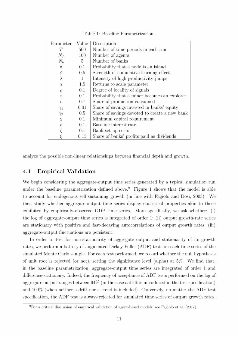
Table 1: Baseline Parametrization.

Parameter Value DescriptionT 500 Number of time periods in each runNf 100 Number of agentsNb 5 Number of banksπ 0.1 Probability that a node is an islandφ 0.5 Strength of cumulative learning effectλ 1 Intensity of high productivity jumpsα 1.5 Returns to scale parameterρ 0.1 Degree of locality of signalsε 0.1 Probability that a miner becomes an explorerc 0.7 Share of production consumedγ1 0.01 Share of savings invested in banks’ equityγ2 0.5 Share of savings devoted to create a new bankχ 0.1 Minimum capital requirementr 0.1 Baseline interest rateζ 0.1 Bank set-up costsξ 0.15 Share of banks’ profits paid as dividends

analyze the possible non-linear relationships between financial depth and growth.

4.1 Empirical Validation

We begin considering the aggregate-output time series generated by a typical simulation run

under the baseline parametrization defined above.9 Figure 1 shows that the model is able

to account for endogenous self-sustaining growth (in line with Fagiolo and Dosi, 2003). We

then study whether aggregate-output time series display statistical properties akin to those

exhibited by empirically-observed GDP time series. More specifically, we ask whether: (i)

the log of aggregate-output time series is integrated of order 1; (ii) output growth-rate series

are stationary with positive and fast-decaying autocorrelations of output growth rates; (iii)

aggregate-output fluctuations are persistent.

In order to test for non-stationarity of aggregate output and stationarity of its growth

rates, we perform a battery of augmented Dickey-Fuller (ADF) tests on each time series of the

simulated Monte Carlo sample. For each test performed, we record whether the null hypothesis

of unit root is rejected (or not), setting the significance level (alpha) at 5%. We find that,

in the baseline parametrization, aggregate-output time series are integrated of order 1 and

difference-stationary. Indeed, the frequency of acceptance of ADF tests performed on the log of

aggregate output ranges between 94% (in the case a drift is introduced in the test specification)

and 100% (when neither a drift nor a trend is included). Conversely, no matter the ADF test

specification, the ADF test is always rejected for simulated time series of output growth rates.

9For a critical discussion of empirical validation of agent-based models, see Fagiolo et al. (2017).

11

Figure 1: Representative time series of log GDP (log(Qt)) generated by the model under thebaseline parametrization in Table 1.

We turn now to analyzing the autocorrelation patterns displayed by the growth rates of

aggregate output. Figure 2 plots MC averages of the autocorrelation function, which we have

separately estimated in each Monte Carlo run. In line with the empirical evidence (Cochrane,

1988), autocorrelations are positive for the first lags and then they fast decay to values not

significantly different from zero —according to Bartlett bands.

Finally, we consider the non-parametric measures V k and Ak(1) of persistence in output

fluctuations used in Campbell and Mankiw (1989) and Cochrane (1988),10 defined as:

V k =T − kT

[1 + 2

k∑j=1

(1− j

k + 1

)rj

],

where rj is the lag j sample estimate of the autocorrelation function, and

Ak(1) =

√V k

1− r21.

Table 2 shows the MC averages and standard errors of the two statistics computed over our arti-

ficial sample. The estimates are significantly larger than one for every time-horizon considered,

confirming that the model is able to produce aggregate-output fluctuations with persistence

levels similar to those observed in real-world GDP data.

The foregoing results suggest that, at least in the baseline parametrization, the model is

able to generate aggregate-output time series that are statistically not distinguishable from

their real-world counterpart. A similar conclusion holds, in general, whenever the model is

10see Fagiolo and Dosi (2003) for more details

12

Figure 2: MC average growth rate autocorrelation function. Dotted lines are 95% Bartlettconfidence bands. Monte Carlo sample: 3000 replications.

K = 10 K = 20 K = 30 K = 40 K = 50

V k 1.616448 1.706264 1.670570 1.613766 1.563051(0.006743) (0.009113) (0.010663) (0.011879) (0.012843)

Ak(1) 1.281972 1.311785 1.292527 1.264568 1.239006(0.002891) (0.003691) (0.004266) (0.004755) (0.005156)

Table 2: MC averages of the estimated V k and Ak(1) with standard errors in parenthesis.Monte Carlo sample: 3000 replications.

able to produce self-sustaining endogenous growth. This happens —as in the original model—

for quite a large subset of the whole parameter space. As discussed in Fagiolo and Roventini

(2017), the fact that an agent-based model is empirical validated for a non-trivial subset of

all its possible parameter constellations is a necessary prerequisite to subsequently ask what-if

type of questions and to perform economic policy exercises.

4.2 The Impact of Credit on Output Growth and Volatility

We begin asking whether introducing banks in the FDM has a positive impact on aggregate

output. We study two setups, one with banks providing credit to firms and the other without

banks, i.e. a sort of ‘autarkic’ setting where firms can rely only on their cumulated cash flows

to finance innovation and imitation activities.

We compare the performance of the simulated economy in the two setups. We focus on

the behavior of (the log of) aggregate output time series, as well growth-rate output volatility.

To measure volatility, we build the time series of the standard deviation of aggregate-output

13

growth rates in the 100 periods preceding the current time step t, i.e.:

σ100t (g) =

√√√√ 99∑τ=0

(gt−τ − µ100t (g))

2

100, (7)

where gt = logQt − logQt−1 and µ100t (g) = (logQt − logQt−100)/100.

The results of our experiments are presented in Figure 3. We observe that the presence

of a banking sector allows for higher growth and lower volatility. This is so because, in the

model, growth stems from a right balance between the resources devoted to producing by

exploiting the current set of technologies, introducing new techniques and diffusing the new

technologies. The credit activity of banks removes the resource constraint preventing agents to

discover new technologies and imitate better ones. This in turn puts the economy on a virtuous

growth path. The growth-enhancing effect of credit is particularly relevant in the first phases of

economic development, when firms need to accumulate enough resources to start exploring the

technological space (see the left panel of Figure 3). The discovery of more productive islands

allows for imitation and this induces the diffusion of better technologies and faster growth. Even

after the economy stabilizes on a steady growth path, the output gap between the scenario with

banks and the ‘autarkic’ setup keeps on increasing, suggesting that the resource constraint does

affect firms when the financial sector is not present.

Let us now consider the impact of banks and credit on output volatility. Figure 3 shows

that volatility is typically high in the first periods of the simulation, and then quickly converges

to its long-run stable value. This points out that the model gets out of its transient phase

quite fast and then reaches its long-run stable growth pattern. The presence of banks appears

to reduce output volatility. Again, the positive influence of the credit sector stems from the

delicate balance between exploration and exploitation, together with the possible emergence

of coordination failures. Indeed, when a firm leaves her island, production falls, and output

can increase again only when a new (highly-productive) island is discovered. If agents move

in a coordinated way, a huge drop in output will be followed by spurs of growth when new

technologies are discovered and diffused. Banks break such a vicious cycle allowing agents to

leave their island smoothly without the accumulation of the resources otherwise needed in the

‘autarkic’ scenario.

4.3 Financial Depth, Output Growth, and Volatility

The foregoing first set of experiments suggests that credit and banks have a positive impact on

growth. This in line with many empirical works (King and Levine, 1993a; Rajan and Zingales,

1998; Levine et al., 2000; Beck et al., 2000).

A natural subsequent question is whether increasing levels of financialization are always

beneficial for growth, or if instead they might harm the economy and, when financialization

14

Figure 3: MC averages of log GDP and 100-period growth rate volatility with and withoutbanking sector. Confidence bands are set to three standard errors away from Monte Carlosample averages.

becomes too strong, can possibly trigger crises. In fact, non-linear relationships in the finance-

growth nexus have been recently found by several studies. For example, Cecchetti and Khar-

roubi (2012); Law and Singh (2014); Arcand et al. (2015) all suggest that the positive effects

of finance tend to vanish after some point, and can even become detrimental as the level of

financial depth increases and goes beyond some thresholds.

In the next experiments, we will explore with our model the existence of non-linearities in

the relationship between finance and growth. We define financial depth —in line with existing

literature (see e.g. Arcand et al., 2015)— as the amount of outstanding loans over production:

FDt =

Nb∑l=1

Ll,t

Qt

. (8)

Since loans provided in the current period may take several time steps to affect growth, we

consider its 10-year average:

FD10

t =

9∑τ=0

FDt−τ

10. (9)

In our regression exercises, the dependent variable is the 10-year output growth rate, defined

as:

G10t = log(Qt)− log(Qt−10) . (10)

To avoid any possible endogeneity issue, we use as a covariate the average financial depth with

a ten-year lag (i.e. FD10

t−10), together with its square.

We build a Monte Carlo sample considering 3000 independent runs, wherein we record FD10

t

and G10t for the last 300 periods of the simulations to avoid any possible transient behaviors.

15

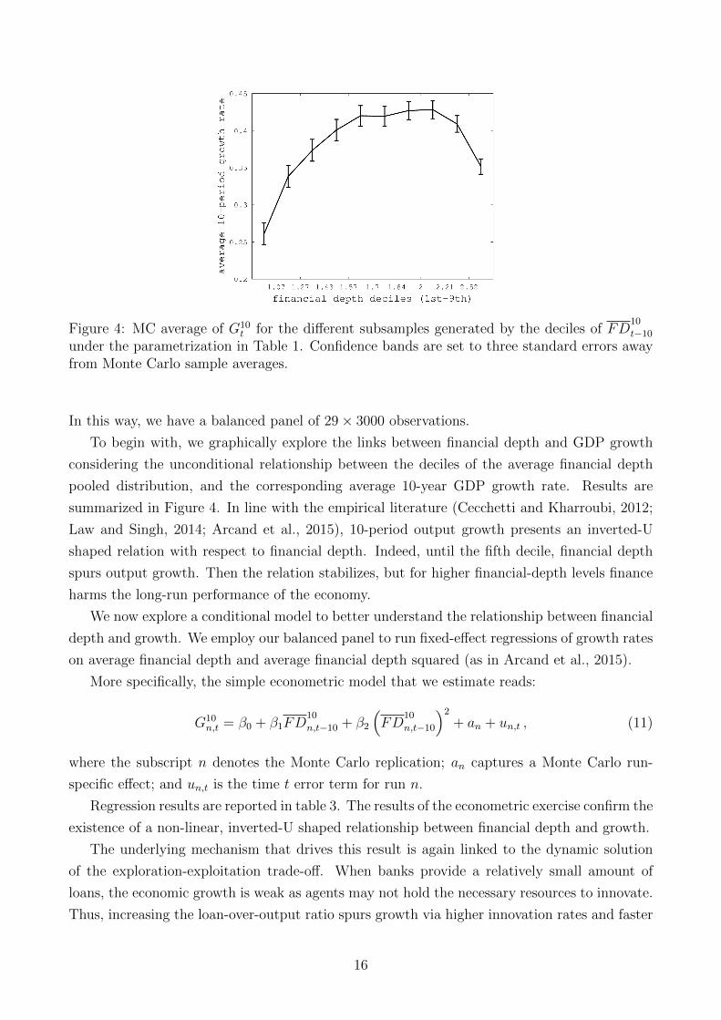
Figure 4: MC average of G10t for the different subsamples generated by the deciles of FD

10

t−10

under the parametrization in Table 1. Confidence bands are set to three standard errors awayfrom Monte Carlo sample averages.

In this way, we have a balanced panel of 29× 3000 observations.

To begin with, we graphically explore the links between financial depth and GDP growth

considering the unconditional relationship between the deciles of the average financial depth

pooled distribution, and the corresponding average 10-year GDP growth rate. Results are

summarized in Figure 4. In line with the empirical literature (Cecchetti and Kharroubi, 2012;

Law and Singh, 2014; Arcand et al., 2015), 10-period output growth presents an inverted-U

shaped relation with respect to financial depth. Indeed, until the fifth decile, financial depth

spurs output growth. Then the relation stabilizes, but for higher financial-depth levels finance

harms the long-run performance of the economy.

We now explore a conditional model to better understand the relationship between financial

depth and growth. We employ our balanced panel to run fixed-effect regressions of growth rates

on average financial depth and average financial depth squared (as in Arcand et al., 2015).

More specifically, the simple econometric model that we estimate reads:

G10n,t = β0 + β1FD

10

n,t−10 + β2

(FD

10

n,t−10

)2+ an + un,t , (11)

where the subscript n denotes the Monte Carlo replication; an captures a Monte Carlo run-

specific effect; and un,t is the time t error term for run n.

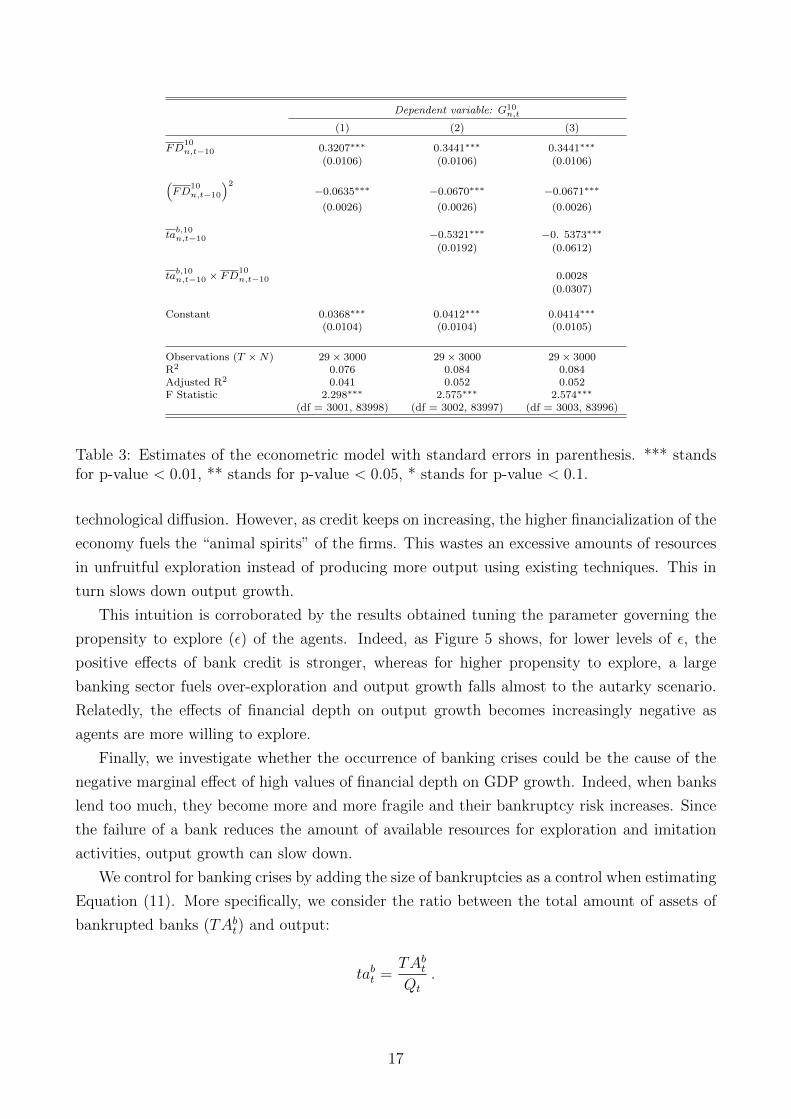
Regression results are reported in table 3. The results of the econometric exercise confirm the

existence of a non-linear, inverted-U shaped relationship between financial depth and growth.

The underlying mechanism that drives this result is again linked to the dynamic solution

of the exploration-exploitation trade-off. When banks provide a relatively small amount of

loans, the economic growth is weak as agents may not hold the necessary resources to innovate.

Thus, increasing the loan-over-output ratio spurs growth via higher innovation rates and faster

16

Dependent variable: G10n,t

(1) (2) (3)

FD10n,t−10 0.3207∗∗∗ 0.3441∗∗∗ 0.3441∗∗∗

(0.0106) (0.0106) (0.0106)(FD

10n,t−10

)2−0.0635∗∗∗ −0.0670∗∗∗ −0.0671∗∗∗

(0.0026) (0.0026) (0.0026)

tab,10n,t−10 −0.5321∗∗∗ −0. 5373∗∗∗

(0.0192) (0.0612)

tab,10n,t−10 × FD

10n,t−10 0.0028

(0.0307)

Constant 0.0368∗∗∗ 0.0412∗∗∗ 0.0414∗∗∗

(0.0104) (0.0104) (0.0105)

Observations (T ×N) 29× 3000 29× 3000 29× 3000R2 0.076 0.084 0.084Adjusted R2 0.041 0.052 0.052F Statistic 2.298∗∗∗ 2.575∗∗∗ 2.574∗∗∗

(df = 3001, 83998) (df = 3002, 83997) (df = 3003, 83996)

Table 3: Estimates of the econometric model with standard errors in parenthesis. *** standsfor p-value < 0.01, ** stands for p-value < 0.05, * stands for p-value < 0.1.

technological diffusion. However, as credit keeps on increasing, the higher financialization of the

economy fuels the “animal spirits” of the firms. This wastes an excessive amounts of resources

in unfruitful exploration instead of producing more output using existing techniques. This in

turn slows down output growth.

This intuition is corroborated by the results obtained tuning the parameter governing the

propensity to explore (ε) of the agents. Indeed, as Figure 5 shows, for lower levels of ε, the

positive effects of bank credit is stronger, whereas for higher propensity to explore, a large

banking sector fuels over-exploration and output growth falls almost to the autarky scenario.

Relatedly, the effects of financial depth on output growth becomes increasingly negative as

agents are more willing to explore.

Finally, we investigate whether the occurrence of banking crises could be the cause of the

negative marginal effect of high values of financial depth on GDP growth. Indeed, when banks

lend too much, they become more and more fragile and their bankruptcy risk increases. Since

the failure of a bank reduces the amount of available resources for exploration and imitation

activities, output growth can slow down.

We control for banking crises by adding the size of bankruptcies as a control when estimating

Equation (11). More specifically, we consider the ratio between the total amount of assets of

bankrupted banks (TAbt) and output:

tabt =TAbtQt

.

17

Figure 5: Propensity to explore parameter ε and economic dynamics. Left: low, ε = 0.05. Mid:

baseline, ε = 0.1. Right: high, ε = 0.12. Top: MC average of log GDP with a banking sector (Nb = 5)

and without (Nb = 0). Bottom: MC average of G10t for the different subsamples generated by the

deciles of FD10t−10. Confidence bands are set as three standard errors away from Monte Carlo sample

averages.

Thus we add to the regression its 10-year average, in order to keep consistency with the econo-

metric model in (11):

tab,10t =

9∑τ=0

tabτ

10.

We also control for possible interaction effects repeating the estimation with the product

between tab,10t−10 and FD

10

n,t−10 among the regressors.

We find that the estimates of financial-depth coefficients do not basically change (cf. Table

3), while the one related to banking crises is negative and significant. Bank bankruptcies

exerts a negative effect on future output growth rates, but they cannot explain the non-linear

relationship between financial depth and output. This is in line with the findings of Arcand

et al. (2015) about the robustness of the inverted-U shaped relation between the two variables

has to financial instability.

4.4 Innovation and Credit

Is there any interaction between the technological engine of the model and the amount of

fuel provided by bank credit? In order to further explore the connection between innovation

and credit, we investigate how our results change when different credit and technical-change

18

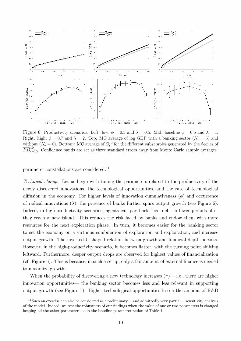
Figure 6: Productivity scenarios. Left: low, φ = 0.3 and λ = 0.5. Mid: baseline φ = 0.5 and λ = 1.

Right: high, φ = 0.7 and λ = 2. Top: MC average of log GDP with a banking sector (Nb = 5) and

without (Nb = 0). Bottom: MC average of G10t for the different subsamples generated by the deciles of

FD10t−10. Confidence bands are set as three standard errors away from Monte Carlo sample averages.

parameter constellations are considered.11

Technical change. Let us begin with tuning the parameters related to the productivity of the

newly discovered innovations, the technological opportunities, and the rate of technological

diffusion in the economy. For higher levels of innovation cumulativeness (φ) and occurrence

of radical innovations (λ), the presence of banks further spurs output growth (see Figure 6).

Indeed, in high-productivity scenarios, agents can pay back their debt in fewer periods after

they reach a new island. This reduces the risk faced by banks and endow them with more

resources for the next exploration phase. In turn, it becomes easier for the banking sector

to set the economy on a virtuous combination of exploration and exploitation, and increase

output growth. The inverted-U shaped relation between growth and financial depth persists.

However, in the high-productivity scenario, it becomes flatter, with the turning point shifting

leftward. Furthermore, deeper output drops are observed for highest values of financialization

(cf. Figure 6). This is because, in such a setup, only a fair amount of external finance is needed

to maximize growth.

When the probability of discovering a new technology increases (π) —i.e., there are higher

innovation opportunities— the banking sector becomes less and less relevant in supporting

output growth (see Figure 7). Higher technological opportunities lessen the amount of R&D

11Such an exercise can also be considered as a preliminary —and admittedly very partial— sensitivity analysisof the model. Indeed, we test the robustness of our findings when the value of one or two parameters is changedkeeping all the other parameters as in the baseline parameterization of Table 1.

19

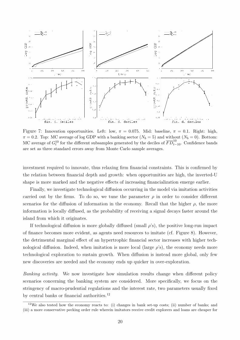
Figure 7: Innovation opportunities. Left: low, π = 0.075. Mid: baseline, π = 0.1. Right: high,

π = 0.2. Top: MC average of log GDP with a banking sector (Nb = 5) and without (Nb = 0). Bottom:

MC average of G10t for the different subsamples generated by the deciles of FD

10t−10. Confidence bands

are set as three standard errors away from Monte Carlo sample averages.

investment required to innovate, thus relaxing firm financial constraints. This is confirmed by

the relation between financial depth and growth: when opportunities are high, the inverted-U

shape is more marked and the negative effects of increasing financialization emerge earlier.

Finally, we investigate technological diffusion occurring in the model via imitation activities

carried out by the firms. To do so, we tune the parameter ρ in order to consider different

scenarios for the diffusion of information in the economy. Recall that the higher ρ, the more

information is locally diffused, as the probability of receiving a signal decays faster around the

island from which it originates.

If technological diffusion is more globally diffused (small ρ’s), the positive long-run impact

of finance becomes more evident, as agents need resources to imitate (cf. Figure 8). However,

the detrimental marginal effect of an hypertrophic financial sector increases with higher tech-

nological diffusion. Indeed, when imitation is more local (large ρ’s), the economy needs more

technological exploration to sustain growth. When diffusion is instead more global, only few

new discoveries are needed and the economy ends up quicker in over-exploration.

Banking activity. We now investigate how simulation results change when different policy

scenarios concerning the banking system are considered. More specifically, we focus on the

stringency of macro-prudential regulations and the interest rate, two parameters usually fixed

by central banks or financial authorities.12

12We also tested how the economy reacts to: (i) changes in bank set-up costs; (ii) number of banks; and(iii) a more conservative pecking order rule wherein imitators receive credit explorers and loans are cheaper for

20

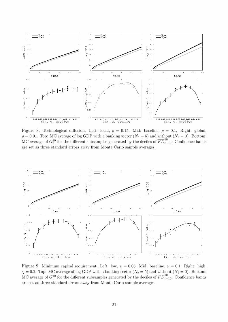
Figure 8: Technological diffusion. Left: local, ρ = 0.15. Mid: baseline, ρ = 0.1. Right: global,

ρ = 0.01. Top: MC average of log GDP with a banking sector (Nb = 5) and without (Nb = 0). Bottom:

MC average of G10t for the different subsamples generated by the deciles of FD

10t−10. Confidence bands

are set as three standard errors away from Monte Carlo sample averages.

Figure 9: Minimum capital requirement. Left: low, χ = 0.05. Mid: baseline, χ = 0.1. Right: high,

χ = 0.2. Top: MC average of log GDP with a banking sector (Nb = 5) and without (Nb = 0). Bottom:

MC average of G10t for the different subsamples generated by the deciles of FD

10t−10. Confidence bands

are set as three standard errors away from Monte Carlo sample averages.

21

Figure 10: Interest rate. Left: low, r = 0.05. Mid: baseline, r = 0.1. Right: high, r = 0.15. Top:

MC average of log GDP with a banking sector (Nb = 5) and without (Nb = 0). Bottom: MC average

of G10t for the different subsamples generated by the deciles of FD

10t−10. Confidence bands are set as

three standard errors away from Monte Carlo sample averages.

More stringent macro-prudential regulations are obtained in the model increasing the min-

imum capital requirement χ. Results show that increasing χ has a positive impact on long-

run growth (see Figure 9). Indeed, restraining credit supply reduces the possibility of over-

exploration, thus reinforcing the balance sheets of banks. This is also confirmed by the relation

between financial depth and growth.

The economy is instead less reactive to changes in the interest rate (r). This is probably

because, on the one hand, higher interest rates extend the period required by firm to pay back

their debt, reducing the long-run output level. However, this effect is counterbalanced by the

fact that firm innovation and imitation decisions in the model do not rely upon the interest

rate.

5 Conclusions

In this paper, we have investigated the interactions between innovation, credit and growth in

a supply-side model of industry dynamics. To do so, we have introduced a banking sector

in the endogenous-growth agent-based model developed in Fagiolo and Dosi (2003). We have

explicitly taken into account the effects that finance has on innovation and imitation activities

imitation than they are for exploration. Overall, our results are robust and consistent with the effect of crediton the exploration-exploitation trade-off. For this reason we do not report such analyses, which are neverthelessavailable from the Authors upon request.

22

of firms, as well as on the long-run performance of the economy.

Simulation results show that banks, by providing loans, are able to foster technological

innovation and diffusion, thus improving long-run economic growth. Credit allows indeed to

achieve a better balance between the technological exploration and exploitation activities of

firms. However, credit and technical change co-evolve with possibly non-linear effects. In line

with the empirical evidence (Cecchetti and Kharroubi, 2012; Law and Singh, 2014; Arcand et al.,

2015), we find an inverted U-shaped relationship between financial depth and output growth.

When firms do not search enough for new technologies, increasing the relative amount of loans

results in higher innovation and faster technological diffusion, thus spurring GDP growth.

However, excessive levels of credit sustain the animal spirits of firm engaged in unfruitful

exploration undermining production and savings.

Overall, this suggests that the interaction between innovation and finance may play a more

fundamental role in fueling growth than previously thought.

The current model could be extended in several ways. First, one could endogeneize the

formation of links between banks and firms. In the basic version of the model, we exogenously

select bank-firm links once and for all before simulations start. Instead, one could allow firm

to strategically switch among different banks or to hold multiple credit lines.

Second, an interbank lending market could be introduced in order to allow banks to extend

loans to one another for a number of time steps.

Finally, on the policy side, one could study the impact of more sophisticated macro-

prudential regulation and the role of patient finance, introducing, e.g., a public investment

bank.

Acknowledgments

G.F., D.G. and A.R. gratefully acknowledge support by the European Union’s Horizon 2020

research and innovation program under grant agreement No. 640772-DOLFINS. G.F. and A.R.

gratefully acknowledge support by the European Union’s Horizon 2020 research and innovation

program under grant agreement No. 649186-ISIGrowth. Thanks to Marina Mastrorillo, Tom-

maso Ferraresi, and Delio Panaro for their contribution to the development of the ideas behind

this version of the model.

References

Acemoglu, D. and F. Zilibotti (1997). Was prometheus unbound by chance? risk, diversification,and growth. Journal of political economy 105 (4), 709–751.

Allen, F. and D. Gale (1997). Financial markets, intermediaries, and intertemporal smoothing.Journal of political Economy 105 (3), 523–546.

Arcand, J. L., E. Berkes, and U. Panizza (2015). Too much finance? Journal of EconomicGrowth 20 (2), 105–148.

23

Arribas, I., J. Peiro-Palomino, and E. Tortosa-Ausina (2017). Is full banking integration desir-able? Journal of Banking & Finance, In Press.

Bagehot, W. (1873). Lombard Street: A description of the money market. Scribner, Armstrong& Company.

Beck, T., B. Buyukkarabacak, F. K. Rioja, and N. T. Valev (2012). Who gets the credit? anddoes it matter? household vs. firm lending across countries. The BE Journal of Macroeco-nomics 12 (1).

Beck, T. and R. Levine (2004). Stock markets, banks, and growth: Panel evidence. Journal ofBanking & Finance 28 (3), 423–442.

Beck, T., R. Levine, and N. Loayza (2000). Finance and the sources of growth. Journal offinancial economics 58 (1), 261–300.

Bencivenga, V. R. and B. D. Smith (1993). Some consequences of credit rationing in anendogenous growth model. Journal of economic Dynamics and Control 17 (1-2), 97–122.

Benczur, P., S. Karagiannis, and V. Kvedaras (2017). Finance and economic growth: financ-ing structure and non-linear impact. Technical report, Joint Research Centre, EuropeanCommission (Ispra site).

Bodenhorn, H. (2016). Two centuries of finance and growth in the united states, 1790-1980.Technical report, National Bureau of Economic Research.

Boyd, J. H. and E. C. Prescott (1986). Financial intermediary-coalitions. Journal of EconomicTheory 38 (2), 211–232.

Campbell, J. Y. and N. G. Mankiw (1989). International evidence on the persistence of economicfluctuations. Journal of Monetary Economics 23 (2), 319–333.

Capolupo, R. (2017). Finance, investment and growth: Evidence for italy. Economic Notes, InPress.

Cecchetti, S. G. and E. Kharroubi (2012). Reassessing the impact of finance on growth. BISWorking Papers 381, Bank for International Settlements.

Cecchetti, S. G. and E. Kharroubi (2015). Why does financial sector growth crowd out realeconomic growth? BIS Working Papers 490, Bank for International Settlements.

Cochrane, J. H. (1988). How big is the random walk in gnp? Journal of political economy 96 (5),893–920.

De la Fuente, A. and J. Marın (1996). Innovation, bank monitoring, and endogenous financialdevelopment. Journal of Monetary Economics 38 (2), 269–301.

Dosi, G. (1988). Sources, procedures, and microeconomic effects of innovation. Journal ofeconomic literature 26, 1120–1171.

Dosi, G., G. Fagiolo, M. Napoletano, and A. Roventini (2013). Income distribution, creditand fiscal policies in an agent-based keynesian model. Journal of Economic Dynamics andControl 37 (8), 1598–1625.

24

Dosi, G., G. Fagiolo, M. Napoletano, A. Roventini, and T. Treibich (2015). Fiscal and monetarypolicies in complex evolving economies. Journal of Economic Dynamics and Control 52, 166–189.

Dosi, G., G. Fagiolo, and A. Roventini (2010). Schumpeter meeting keynes: A policy-friendlymodel of endogenous growth and business cycles. Journal of Economic Dynamics and Con-trol 34 (9), 1748–1767.

Dosi, G. and D. Lovallo (1997). Rational entrepreneurs or optimistic martyrs? Some considera-tions on technological regimes, corporate entries, and the evolutionary role of decision biases.Cambridge, UK: Cambridge University Press.

Dosi, G. and R. Nelson (1994). An introduction to evolutionary theories in economics. Journalof Evolutionary Economics 4, 153–172.

Dosi, G. and R. R. Nelson (2010). Technological change and industrial dynamics as evolutionaryprocesses. In B. H. Hall and N. Rosenberg (Eds.), Handbook of the Economics of Innovation,Chapter 4. Elsevier: Amsterdam.

Epstein, G. A. (2005). Financialization and the world economy. Edward Elgar Publishing.

Fagiolo, G. and G. Dosi (2003). Exploitation, exploration and innovation in a model of en-dogenous growth with locally interacting agents. Structural Change and Economic Dynam-ics 14 (3), 237–273.

Fagiolo, G., M. Guerini, F. Lamperti, A. Moneta, A. Roventini, et al. (2017). Validation ofagent-based models in economics and finance. Technical report, Laboratory of Economicsand Management (LEM), Sant’Anna School of Advanced Studies, Pisa, Italy.

Fagiolo, G. and A. Roventini (2017). Macroeconomic policy in dsge and agent-based modelsredux: New developments and challenges ahead. Journal of Artificial Societies and SocialSimulation 20 (1), 1.

Greenwood, J. and B. Jovanovic (1990). Financial development, growth, and the distributionof income. Journal of political Economy 98 (5, Part 1), 1076–1107.

Greenwood, J. and B. D. Smith (1997). Financial markets in development, and the developmentof financial markets. Journal of Economic dynamics and control 21 (1), 145–181.

Jerzmanowski, M. (2017). Finance and sources of growth: evidence from the us states. Journalof Economic Growth 22 (1), 97–122.

Kaminsky, G. L. and C. M. Reinhart (1999). The twin crises: the causes of banking andbalance-of-payments problems. American economic review 89, 473–500.

King, R. G. and R. Levine (1993a). Finance and growth: Schumpeter might be right. Thequarterly journal of economics 108 (3), 717–737.

King, R. G. and R. Levine (1993b). Finance, entrepreneurship and growth. Journal of Monetaryeconomics 32 (3), 513–542.

Kneer, C. (2013). Finance as a magnet for the best and brightest: Implications for the realeconomy. Working Paper 392, DNB.

25

Law, S. H. and N. Singh (2014). Does too much finance harm economic growth? Journal ofBanking & Finance 41, 36–44.

LeBaron, B. and L. Tesfatsion (2008). Modeling macroeconomies as open-ended dynamic sys-tems of interacting agents. American Economic Review 98, 246–250.

Levine, R. (1991). Stock markets, growth, and tax policy. The Journal of Finance 46 (4),1445–1465.

Levine, R. (2005). Finance and growth: theory and evidence. Handbook of economic growth 1,865–934.

Levine, R., N. Loayza, and T. Beck (2000). Financial intermediation and growth: Causalityand causes. Journal of monetary Economics 46 (1), 31–77.

Madsen, J. B. and J. B. Ang (2016). Finance-led growth in the oecd since the nineteenthcentury: How does financial development transmit to growth? Review of Economics andStatistics 98 (3), 552–572.

Nelson, R. and S. Winter (1982). An Evolutionary Theory of Economic Change. HarvardUniversity Press.

Nelson, R. and S. Winter (2002). Evolutionary theorizing in economics. Journal of EconomicPerspectives 16, 23–46.

Nyasha, S. and N. M. Odhiambo (2017). Financial development and economic growth nexus:A revisionist approach. Economic Notes, In Press.

Philippon, T. and A. Reshef (2013). An international look at the growth of modern finance.The Journal of Economic Perspectives 27 (2), 73–96.

Rajan, R. G. and L. Zingales (1998). Financial dependence and growth. The American economicreview 88 (3), 559–586.

Robinson, J. (1952). The generalization of the general theory. In J. Robinson (Ed.), The Rateof Interest and Other Essays. London: MacMillan.

Schularick, M. and A. M. Taylor (2012). Credit booms gone bust: monetary policy, leveragecycles, and financial crises, 1870–2008. The American Economic Review 102 (2), 1029–1061.

Schumpeter, J. A. (1911). The Theory of Economic Development. Harvard University Press.

Silverberg, G. and B. Verspagen (1995). Evolutionary theorizing on economic growth. IIASAWorking Papers WP-95-078, IIASA, Laxenburg, Austria.

Sirri, E. and P. Tufano (1995). The economics of pooling. In Crane, D.B., et al. (Eds.), TheGlobal Financial System: A Functional Approach. Harvard Business School Press.

Stiglitz, J. E. and A. Weiss (1981). Credit rationing in markets with imperfect information.The American economic review 71 (3), 393–410.

Stiglitz, J. E. and A. Weiss (1983). Incentive effects of terminations: Applications to the creditand labor markets. The American Economic Review 73 (5), 912–927.

26

Stolbov, M. (2017). Causality between credit depth and economic growth: Evidence from 24oecd countries. Empirical Economics 53 (2), 493–524.

Tesfatsion, L. and K. Judd (Eds.) (2006). Handbook of Computational Economics II: Agent-Based Computational Economics. North Holland, Amsterdam.

27

ABOUT OFCE

The Paris-based Observatoire français des conjonctures économiques (OFCE), or French Economic Observatory is an independent and publicly-funded centre whose activities focus on economic research, forecasting and the evaluation of public policy. Its 1981 founding charter established it as part of the French Fondation nationale des sciences politiques (Sciences Po), and gave it the mission is to “ensure that the fruits of scientific rigour and academic independence serve the public debate about the economy”. The OFCE fulfils this mission by conducting theoretical and empirical studies, taking part in international scientific networks, and assuring a regular presence in the media through close cooperation with the French and European public authorities. The work of the OFCE covers most fields of economic analysis, from macroeconomics, growth, social welfare programmes, taxation and employment policy to sustainable development, competition, innovation and regulatory affairs..

ABOUT SCIENCES PO

Sciences Po is an institution of higher education and research in the humanities and social sciences. Its work in law, economics, history, political science and sociology is pursued through ten research units and several crosscutting programmes. Its research community includes over two hundred twenty members and three hundred fifty PhD candidates. Recognized internationally, their work covers a wide range of topics including education, democracies, urban development, globalization and public health. One of Sciences Po’s key objectives is to make a significant contribution to methodological, epistemological and theoretical advances in the humanities and social sciences. Sciences Po’s mission is also to share the results of its research with the international research community, students, and more broadly, society as a whole.

PARTNERSHIP