EML 6229: Introduction to Random Dynamical Systems

Mrinal Kumar c©

Jan 06, 2016

Initial Impressions and the History of Probability Theory

• The subject of probability has been around for well over two thousand years. Throughthe ages, it has gone through the complete cycle of scholastic evolution - from beingnothing more than pure guesswork, to being at best a half-baked branch of naturalscience meant only for explanation of empirical data, to its present state in which it isa firmly established abstract field of mathematics.

• Even after the rigorous theoretical foundations of probability theory were laid down, itwas not accepted by all in the scientific and mathematics communities as a legitimatefield of mathematics. The primary controversy was one borne out of metaphysicalconcerns - how could the mathematical reality underlying nature be written in thelanguage of chance? Even today, there are researchers who cringe from it, preferring tobelieve in the deterministic view of the universe. A popular example is Albert Einstein,who stated that “God does not play dice”. Ironically, part of the work for which he wonthe Nobel prize (his 1905 seminal paper on Brownian motion) became the foundationfor the mathematical model of white noise , which is used universally for describingrandom perturbations in engineering systems.

• In light of all this fuss, we would first like to know if probability theory is actually alegitimate field of mathematics?! This requires us to ask the following question: Whendoes a field of study become a well-founded branch of mathematics? In other words,what is the mathematical method?

• We have all studied about the scientific method at some point of our educationaltraining: it is an approach of studying nature that involves the following steps:

1. Observation of physical phenomena.

2. Formulation of hypothesis to explain observations.

3. Use of hypothesis to predict future behavior of the observed phenomena.

4. Most important: Continuous testing of the formulated hypothesis by repeatedexperimentation, performed independently by several different researchers.

The above steps qualify without doubt astronomy as a field of science, but reduceastrology to mere speculation. So then, what is the mathematical method? Howshould probability theory be formulated so that it may unequivocally be regarded as afield of mathematics?

• We can say that a set of concepts becomes a well-founded area of mathematics if it hasthe following underlying structure, known as the axiomatic framework :

1

1. At the bottom, it contains a set of “undefinables” which form the very basicbuilding blocks for more sophisticated ideas to follow. These cannot really bedefined, simply because there are no quantities simpler than them in terms ofwhich a definition could be written. Examples include a point, a line, an elementof a set, etc.

2. Using the undefinables, a set of axioms or postulates is laid down. These are “un-deniable” properties. As undefinables cannot be defined, the undeniables cannotbe proved. The axioms result purely from intuition and do not involve mathemat-ical reasoning. It is required that the set of axioms be consistent because they willbe used as the starting point to build the theory. Consistency is very importantin developing axioms.

3. Using the axioms, logic is employed to develop the theory. Today, this approachis easy to follow because it uses the definition-theorem-proof style. Note thatdefinitions come after the axioms have been laid down.

The above procedure is called the axiomatic approach of mathematics and in fact, ismathematics.

• When there are only axioms and nothing else (not even definitions), we are in therealm of pure abstraction. As we define objects and build theorems using them, westart giving these abstract ideas concrete form. When the number of axioms underlyinga mathematical theory is small, the scope of the concrete results that follow is broad.The best example is set theory - which has the fewest number of axioms. Therefore inset theory alone, there are only a few theorems to prove; but, these theorems are widelyapplicable. Consequently, set theory serves as a precursor to many other branches ofmathematics, including probability theory. As more axioms are added, more and moretheorems can be proved. This results in additional branches of mathematics, such astopology (how close are two sets?), algebra (how can we add two sets?), geometry(topology + algebra) and of course, probability theory. As mentioned above, there area lot more theorems to prove in these new branches of mathematics because there is agreater number of axioms, but their applicability is narrower.

• It was Andrey Nikolaevich Kolmogorov in the early 1930’s, who established prob-ability as a branch of mathematics by building an axiomatic framework for it. Notonly did he formalize the process of computing probabilities, his work led to significantgeneralization of previously held “notions”, making them formally applicable to a muchbroader set of objects. Most significantly, before Kolmogorov’s arrival probability wasonly applicable to countable sets. Under his axiomatic paradigm, it became possible toextend it to uncountable sets as well. This will be of crucial importance to us in thiscourse.

• As the title of this course suggests, we are interested in studying probability theoryin the context of dynamical systems. The history of dynamical systems can be tracedall the way back to Isaac Newton and his Newtonian mechanics. We will mostly beconcerned with dynamical systems evolving in continuous time, a general mathematical

2

model for which can be given by the following vector differential equation:

x = f(t,x) (1)

where, x ∈ <N is called the state of the dynamical system. The vector functionf(t,x) : [0,∞)×<N → <N has desirable properties of smoothness. Note that Eq.1 is aset of N first order ordinary differential equations (ODE’s). This form of a dynamicalsystem is called its state-space form. For example, consider a damped linear spring:

x+ cx+ kx = 0 (2)

The above equation represents a dynamical system model for a linear spring damperassembly, where x is the difference between the current and the natural lengths of thespring. Note that Eq.2 is not in state-space form, because it is a second-order ODE.In order to reduce it to state-space form, we have the following developments:

x1 = x2 (3a)

x2 = −cx2 − kx1 (3b)

In the above equations, we have defined new states x1.= x and x2

.= x. This allows

us to reduce the second order ODE of Eq.2 to two first order ODE’s. We thus get thestate-space form, and x1 and x2 are the two states of the spring-damper system. Interms of physics, note that they correspond to position and velocity respectively. Thetwo equations can be written together in vector form as follows:{

x1x2

}=

{x2

−cx2 − kx1

} (=

{f1f2

})(4)

The above system is of the type given in Eq.1, with x = {x1, x2} ∈ <2.

• What is missing in the dynamical system model of Eq.1? This is a typical questionasked in every introductory lecture on mechanics! An ODE is written down, followingwhich the instructor asks with excitement - what did I miss? And someone gives theanswer with a bored look on their face - the initial conditions..

• Indeed, initial conditions are required to complete the description. Let us thereforewrite the whole thing again:

x = f(t,x), x(t = t0) = x0 (5)

The solution to the above equation is given by:

x(t) = x0 +

∫ t

t0

f(τ,x)dτ (6)

• The above model of a physical process is called a deterministic dynamical system.It is called deterministic because complete knowledge about the states can be obtainedfor all times, i.e. x(t) ∀t ∈ [t0,∞), without any room for doubt or uncertainty. Thisassumes the following:

3

1. Eq.5 captures the complete description of the dynamical system. There are noother residual disturbing forces such as “noise” left unmodeled.

2. The precise value of the initial conditions, i.e. x(t0) is known.

3. All the system’s parameters are known without any uncertainty. In the discussedmodel of a linear spring, we have two parameters: c and k. Both of them shouldbe known perfectly.

4. The integral in Eq.6 can be computed, either analytically or numerically.

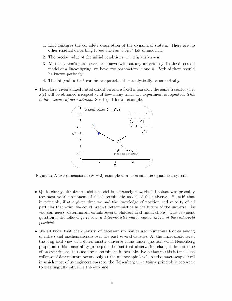
• Therefore, given a fixed initial condition and a fixed integrator, the same trajectory i.e.x(t) will be obtained irrespective of how many times the experiment is repeated. Thisis the essence of determinism. See Fig. 1 for an example.

Dynamical system:

(“Phase-space trajectory”)

Figure 1: A two dimensional (N = 2) example of a deterministic dynamical system.

• Quite clearly, the deterministic model is extremely powerful! Laplace was probablythe most vocal proponent of the deterministic model of the universe. He said thatin principle, if at a given time we had the knowledge of position and velocity of allparticles that exist, we could predict deterministically the future of the universe. Asyou can guess, determinism entails several philosophical implications. One pertinentquestion is the following: Is such a deterministic mathematical model of the real worldpossible?

• We all know that the question of determinism has caused numerous battles amongscientists and mathematicians over the past several decades. At the microscopic level,the long held view of a deterministic universe came under question when Heisenbergpropounded his uncertainty principle - the fact that observation changes the outcomeof an experiment, thus making determinism impossible. Even though this is true, suchcollapse of determinism occurs only at the microscopic level. At the macroscopic levelin which most of us engineers operate, the Heisenberg uncertainty principle is too weakto meaningfully influence the outcome.

4

• In this course, we will look at macroscopic systems and study how the deterministicview of the universe is inadequate or impractical for them.

• What are the possible sources of uncertainty in a macroscopic dynamical system? Itwill be useful to re-examine the list given in Pg. 4 as conditions of determinism, whilealso looking at Eq.5. First, let us consider only the first two items on this list. Whenitems 1 and 2 in the list fail, we obtain the following two main sources of uncertainty:

1. Presence of random perturbations, or, noise in the system, which directly influ-ences the evolution of state dynamics. This perturbation is present in addition tothe “deterministic part” of the model, namely f(t,x). For now, we are assumingeverything about the function f(t,x) is completely known.

2. It is also possible that the initial conditions are not known precisely. In real life,this is typically the result of imperfect measurements.

• The deterministic dynamical system model of Eq.5 can now be expanded to includethe two sources of uncertainty described above. For simplicity, let us first consider thecase of a scalar state-space (N = 1):

x = f(t, x) + ζ(t), W(t0, x) =W0(x) (7)

Written in the above form as an ordinary differential equation with a deterministic partand a non-deterministic “noise” part, Eq.7 is called a Langevin equation. In Eq.7,ζ(t) represents “noise”, a random perturbation typically much smaller in magnitudethan the deterministic force f . A typical comparison of relative magnitudes is shownin Fig.2(a). The symbol W is explained below in Pg. 6.

• We will learn in this course that it is not easy to model the random force ζ(t). Ithas many exotic properties, the most intriguing of which is that it is impossible togenerate the same time-history of noise in two separate runs of an experiment, evenunder the exact same conditions and the same initial conditions. Each time-historycan be referred to as a “noise sample”. Obviously, this is a body blow to the concept ofdeterminism on the macroscopic scale. Every time we run the experiment, the randomforces driving the system will be slightly different, thus making it impossible to makedefinitive predictions about the future of the dynamical process. This situation isshown in Fig.2(b), where three integrations starting from the same initial conditionsgive three different time histories of the state. The noise sample for each run of thenumerical experiment is also shown. For these figures, do not bother with the numberson the y-axis. Just concentrate on the qualitative nature of the plots. The point isthat different runs give different results despite using the same integrator and the sameinitial conditions.

• The second source of uncertainty mentioned above is the lack of precise knowledge ofinitial conditions. This form of uncertainty is fairly common and makes physical sense.No instrument is perfect and therefore it is never possible to know exactly what valuesthe state has at t0. We can at best provide a probabilistic description. I.E., insteadof specifying the initial value of the state as x(t0) = x0, we say that the probability

5

(a) Typical relative magnitudes of the determin-istic force and noise

Noise Driven Trajectories

The solid red line shows thepurely deterministic trajectory,i.e. in the absence of noise.

No

ise:

No

ise:

N

ois

e:

Stat

e:

Stat

e:

Stat

e:

Experiment 1 Experiment 2

Experiment 3

(b) Noise samples are always different in differentruns of the same experiment

Figure 2: The first source of uncertainty in dynamical systems: random perturbations.

density function (pdf) of the state at t0 is W(t0, x) = W0(x). A typical output ofan instrument used to measure the initial conditions is shown in Fig.3(a). The yellowcircle is the “average” value of all possible initial states.

• A pdf is very much like a mass density function. You know that integrating the massdensity over a volume V gives the mass of the object contained in the volume V .Similarly, integrating the pdf of the state over a region A of the state-space gives usthe probability of the state assuming some value in the region A:

P (x0 ∈ A) =

∫AW0(x)dx (8)

We will obviously elaborate more on the above equation in class. For now, you needto know that at t0, the state could actually have any value in <N , and the probabilityof it being in a particular region can be computed by integrating its initial probabilitydensity function.

• The pdf of the state at t0, i.e. W0(x) will depend on the characteristics of the instrumentused to measure the initial conditions. We will learn about many different types of pdf’s.The most common and perhaps the most important is the Gaussian pdf. A Gaussianpdf in two dimensions is shown in Fig.3(b).

6

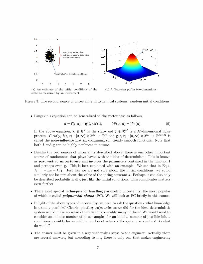
Most likely output of aninstrument used to determinethe initial conditions

“mean value” of the initial conditions

(a) An estimate of the initial conditions of thestate as measured by an instrument.

(b) A Gaussian pdf in two-dimensions.

Figure 3: The second source of uncertainty in dynamical systems: random initial conditions.

• Langevin’s equation can be generalized to the vector case as follows:

x = f(t,x) + g(t,x)ζ(t), W(t0,x) =W0(x) (9)

In the above equation, x ∈ <N is the state and ζ ∈ <M is a M -dimensional noiseprocess. Clearly, f(t,x) : [0,∞) × <N → <N and g(t,x) : [0,∞) × <N → <N×M iscalled the noise-influence matrix, containing sufficiently smooth functions. Note thatboth f and g can be highly nonlinear in nature.

• Besides the two sources of uncertainty described above, there is one other importantsource of randomness that plays havoc with the idea of determinism. This is knownas parametric uncertainty and involves the parameters contained in the function fand perhaps even g. This is best explained with an example. We see that in Eq.4,f2 = −cx2 − kx1. Just like we are not sure about the initial conditions, we couldsimilarly not be sure about the value of the spring constant k. Perhaps it can also onlybe described probabilistically, just like the initial conditions. This complicates matterseven further.

• There exist special techniques for handling parametric uncertainty, the most popularof which is called polynomial chaos (PC). We will look at PC briefly in this course.

• In light of the above types of uncertainty, we need to ask the question - what knowledgeis actually possible? Clearly, plotting trajectories as we did for the ideal deterministicsystem would make no sense - there are uncountably many of them! We would need toconsider an infinite number of noise samples for an infinite number of possible initialconditions, possibly for an infinite number of values of the system parameters! So whatdo we do?

• The answer must be given in a way that makes sense to the engineer. Actually thereare several answers, but according to me, there is only one that makes engineering

7

sense. Mathematicians have tried to give absolute descriptions of the state even insuch hopelessly uncertain settings. There has been some success, but the problem liesin the fact that such descriptions are not very useful, especially to the practitioner.

• When the problem set-up is so inherently probabilistic, it makes perfect sense to giveestimates about the system that are also probabilistic. This can mean only one thing -instead of trying to solve for the time varying state of the system, i.e. x(t); solve for itstime varying probabilistic description. This will obviously need a lot of explaining. Butfirst, it will require an understanding of what we mean by probabilistic descriptions. Aglimpse was given when we talked about the probability density function, or the pdf.We looked at the probability density of the state at time t0, which we called W(t0, x).Then, the complete probabilistic information about the state of the random dynamicalsystem, influenced by one or more of the described forms of uncertainty can be obtainedby computing the probability density function of the state at all times, i.e. W(t, x).This will always be the ultimate objective.

• In summary, we are attempting to bring together two separate fields in this course -dynamical systems and probability theory. Before we proceed to the technical details,it is important to learn a little about the history of probability theory:

– BC era: Both in Greece and Rome, games of chance were popular. However, therewas no scientific or mathematical development of the subject. It is speculatedthat the main reason was the number system used by the Greeks, which was notamenable to algebraic calculations.

– 16th century: Italian mathematician Girolamo Cardano published the first bookcontaining correct methods for calculating the probabilities in games of chanceinvolving dice and cards. Probability was mainly considered an exercise in count-ing.

– 17th century: Work by Fermat and Pascal stirs further interest in the field ofprobability, which was still being studied as a counting of frequencies.

– 18th century: Jacob Bernoulli introduced the first law of large numbers afterstudying repeated coin tossing experiments. This was an important step towardslinking empirical physical reality with conceptual probability. Contributions weremade by several heavyweights of mathematics like Daniel Bernoulli, Leibnitz,Bayes, Lagrange and De Moivre. De Moivre introduced the normal distributionand proved the first form of the central limit theorem.

– 19th century: Laplace published an influential book, firmly establishing the im-portance of probability theory as a quantitative field. He also provided a moregeneral version of the central limit theorem. Legendre and Gauss applied proba-bility to problems in astrodynamics through the method of least squares. Poissondeveloped the Poisson distribution and published an important book with numer-ous original contributions. Chebyshev and his students, Markov and Lyapunovstudied limit theorems, leading to very important results.

8

– Important fact about development of probability theory thus far: In the develop-ment of the theory of probability up to this point, probability was primarily viewedas a natural science, whose primary goal was to explain physical phenomena in thecontext of repeatable experiments. The keyword here is “repeatable”, because sofar probability was considered an exercise in counting and then determining thechance of occurrence as the limit of relative frequencies. This counting approachto probability is today known as the frequentist approach to probability. Notethat this approach relies heavily on empirical support. Also note that with thisapproach, it is possible only to deal with finite sized, or at most countable sets ofdata. Kolmogorov changed all that in the 20th century.

– 20th century: Andrey Kolmogorov is the key figure among several giants whomade contributions to this field. It was Kolmogorov however, who establishedprobability theory as a pure branch of mathematics, thus banishing its status as anatural science. He did this by discarding the empirical frequentist approach de-scribed above and formulating the axiomatic framework of probability. Prob-ability could now be studied as a subject in itself, purely on the basis of logicalcorrectness arising out of the axiomatic structure, and without any dependance onphysical phenomena. This was the turning point for probability theory and todayit has become one of the most theoretically sound and unfortunately, sometimeshighly esoteric fields of mathematics.

• As mentioned above, this course is about the application of probability theory to dy-namical systems. It is therefore important to study that branch of the history as well:

– The first known application of probability theory to dynamical systems was in thefrequentist era (i.e. before Kolmogorov’s seminal work), by well known physicistsMaxwell and Boltzmann in the 1860’s. They were trying to prove that heat ina medium is nothing but the random motion of the constituent gas molecules.With reference to Eq.9, they modeled the system without random perturbation(i.e. g(t,x) = 0) and only initial state uncertainty. Their work culminated in theMaxwell-Boltzmann distribution, which is the steady state distribution of the gasmolecules in an undisturbed medium. Details are available in the 1896 book byBoltzmann. Their work was pioneering, but riddled with annoying paradoxes andinconsistencies. Nonetheless, they were able to account for several properties ofgases.

– Around this time, Rayleigh (1880, 1894), who among other things was also aphysicist, studied (unknowingly) the problem of random walk in two dimen-sional space. He arrived at a partial differential equation describing the evolutionof the displacement of the object performing the random walk. This was lateridentified as the first form of the Fokker-Planck equation (FPE). FPE is avery important equation in the subject of probabilistic mechanics, having someresemblance (philosophically speaking) to Newton’s second law of motion for de-terministic mechanics. We will learn about FPE towards the end of this course.

– French mathematician Bachelier was studying the problem of gambler’s ruin,which is another manifestation of the random walk problem. He obtained a more

9

general form of the Fokker-Planck equation. Note that FPE did not get its nameat this point because neither Fokker nor Planck have yet entered the picture. Itis only in retrospect that we know the equations obtained by Rayleigh, Bachelierand others were nothing but the FPE.

– The stage was set for Albert Einstein, who in 1905 brought together the worksof Maxwell and Boltzmann and the random walk approach to develop the theoryof Brownian motion. He considered the following simplest possible form of arandomly perturbed system:

x = ζ (10)

where, x is the displacement of the fluid particle performing Brownian motion andζ is a random impulse acting on the particle due to collisions with its neighbors.Assuming the displacements to be small, he proceeded to obtain a partial differ-ential equation for the probability density function of x, the displacement of thefluid particle. This was the simplest form of the Fokker-Planck equation. Notethat he was considering only a single dimensional Brownian motion (Eq.10 is ascalar ODE).

– In the meantime, there was another significant contribution by Paul Langevin in1908. He was the first to actually provide Eq.7. In other words, it was his ideato write the dynamics of a randomly perturbed system as an ordinary differentialequation, in which the forces are split into a deterministic part and a randomdisturbance part appearing as an additional forcing function. This served as anamazing clarifying tool for understanding the internal workings of a random dy-namical system. Its power lies in its simplicity. We will later see that Langevin’sdescription of a random dynamical system as a system of ODE’s encounters seri-ous problems of mathematical rigor. Nonetheless, these problems do not changethe fact that it still is a great visualization device for understanding the physicsof the problem.

– In 1914, Adriaan Fokker - part time musician and part time physicist appliedprobability theory to study a first order ODE system with noise and obtaineda partial differential equation. He had considered the general case in which thenoise intensity was dependent on the state of the system. In 1915, Max Planckgeneralized Fokker’s work to vector systems (N > 1 in Eq.9) and applied it toproblems in quantum mechanics. The partial differential equations thatFokker and Planck obtained with the state probability density functionas the unknown was named the Fokker-Planck equation. We will studythis equation in detail. But first, we need to build our background in probabilitytheory and understand what a probability density function is!

– The theory of FPE was greatly enhanced and made more abstract by Kolmogorovand his axiomatic framework of probability. He also talked about the unique-ness of the solutions of FPE. To honor Kolmogorov’s seminal contributions tothis area, the Fokker-Planck equation is also sometimes called the Fokker-Planck-Kolmogorov equation (FPKE), and also Kolmogorov’s first equation.

10

– Since Kolmogorov, the focus on random dynamical systems has been channeledin two main directions: (1) consolidation of the theory of random processes and(2) application of the theory to engineering problems. Notable researchers forthe former are Andronov, Uhlenbeck, Ornstein, Chandrashekhar, Smoluchowski,Stratonovich and more recently, Sean Meyn and Kushner.

– A large number of researchers started applying probability theory to study nonlin-ear random vibration problems in various fields of engineering in the 1960’s. Thoseinterested should look at papers by Caughey, Ariaratnam, Dienes, Crandall andLyon for extremely readable research articles (from the 60’s).

– Another chunk of research effort was directed towards the use of probability theoryto solve problems in control of nonlinear systems perturbed by random forces. Tolearn about the early work in this direction, look for papers by Stratonovich,Bellman, Chuang, Kazda and Barrett from the 1960’s.

– Today, FPE lies at the heart of numerous problems in engineering - for example,structural vibration for mechanical and civil engineering applications; uncertaintypropagation in nonlinear dynamics, including astrodynamics; nonlinear filteringtheory; stochastic control theory; chemical process equilibria; particle physics, etc.

– Unfortunately, we have found that FPE is a formidable problem to tackle. Ana-lytical results have not been found except for the simplest of cases. In the 1970’s,with the advent of moderately powerful computers, numerical attempts were ini-tiated but quickly ran into multiple roadblocks. We will discuss these roadblockslater. For now, it suffices to mention that the biggest obstruction is somethingknown as the curse of dimensionality. In the 70’s, researchers used discretizationtechniques like finite differences (Killeen, Futch, Whitney etc.). In 1985, Langleyused finite elements (FEM) for the first time, which then became the norm forabout 20 years. And more recently, I have used what is known as the meshlessfinite elements technique to correct the shortcomings of FEM for FPE.

– In conclusion, it is important to mention that FPE is the most accurate probabilis-tic description of a continuous random dynamical system modeled by the Langevinequation in Eq.9. Ever since it was discovered that its analytical solution is ex-tremely difficult to obtain, researchers started looking for alternate methods ofanalysis. Some of the popular approximate methods are statistical lineariza-tion, Gaussian closure, higher order moment closures and Monte Carlomethods. Actually, Monte Carlo method is not really an approximate technique- it converges to the true answer (the one that FPE would provide), but only inthe limit as the computation effort tends to infinity. The rate of convergence hasalso been a controversial issue so we will look at Monte Carlo as an approximatetechnique. We will study at least some of these alternate methods in this course.

References:

1. Arch W. Naylor & George R. Sell, Linear Operator Theory in Engineering and Science,Springer Series in Applied Mathematical Sciences # 40, Springer, New York, 1982.ISBN: 0-387-95001-X

11

2. Dimitri Bertsekas & John N. Tsitsiklis, Introduction to Probability, Athena Scientific;2nd edition (July 15, 2008); ISBN-10: 1-88-652923-X

3. H. Risken, The Fokker Planck Equation: Methods of Solution and Applications, SpringerSeries in Synergetics

4. A. T. Fuller, Analysis of Nonlinear Stochastic Systems by Means of the Fokker-PlanckEquation, International Journal of Control , Vol. 9, No. 6, 1969, pp. 603655

12